
Multi-Response Optimization of Abrasive Waterjet Machining of Ti6Al4V Using Integrated Approach of Utilized Heat Transfer Search Algorithm and RSM

 , , , and
Abstract
:1. Introduction
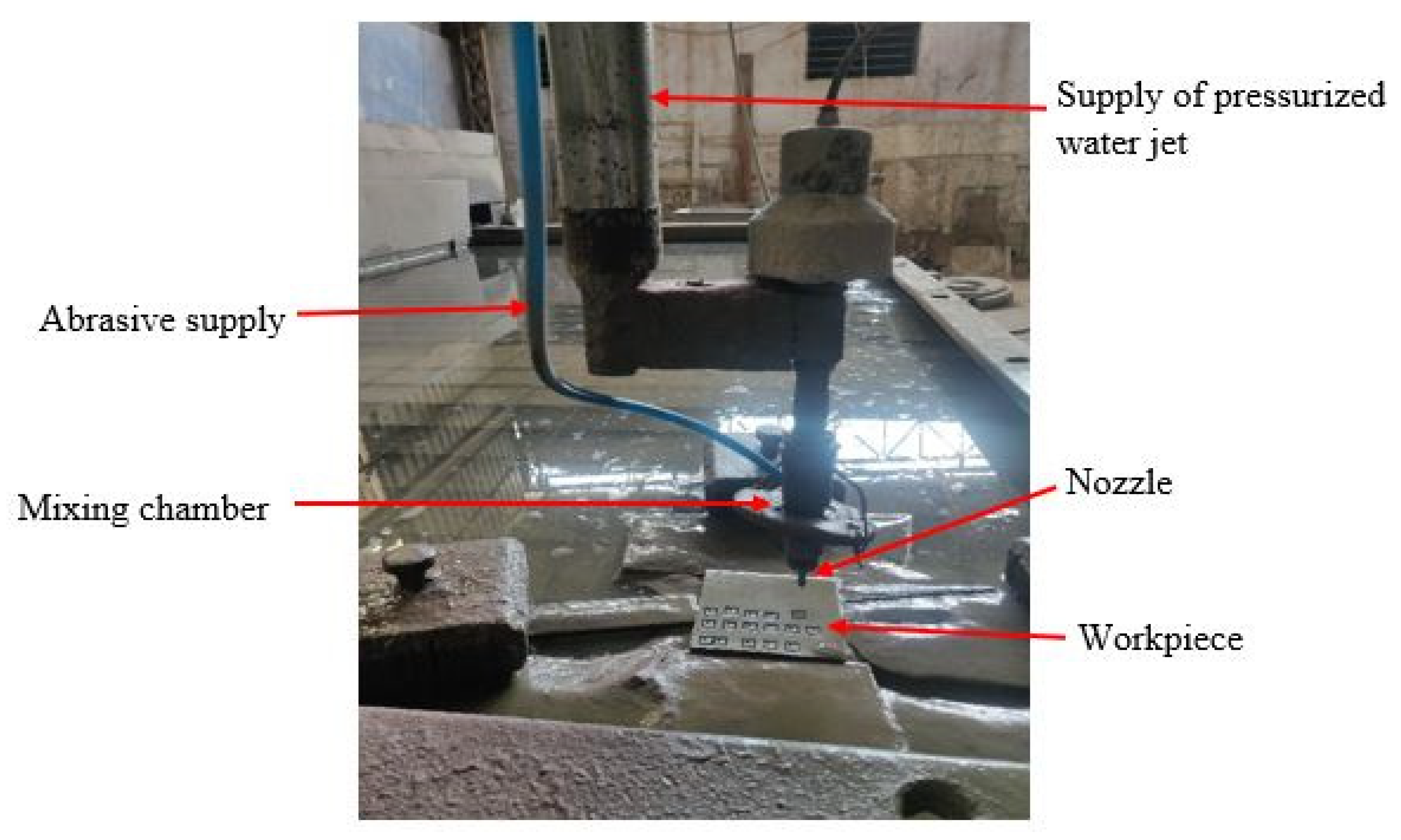
2. Materials and Methods
3. Results and Discussion
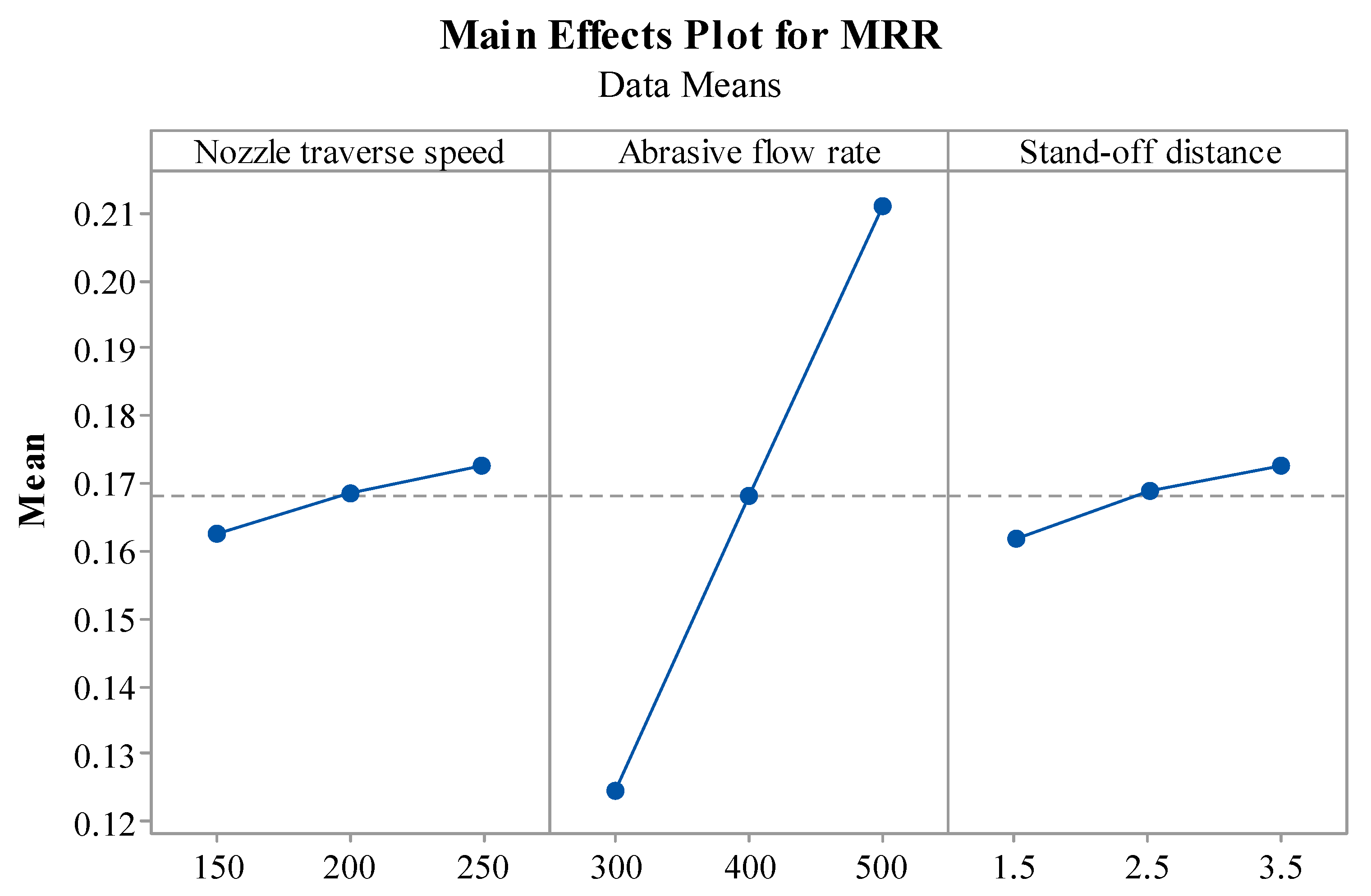
3.1. Analysis of MRR
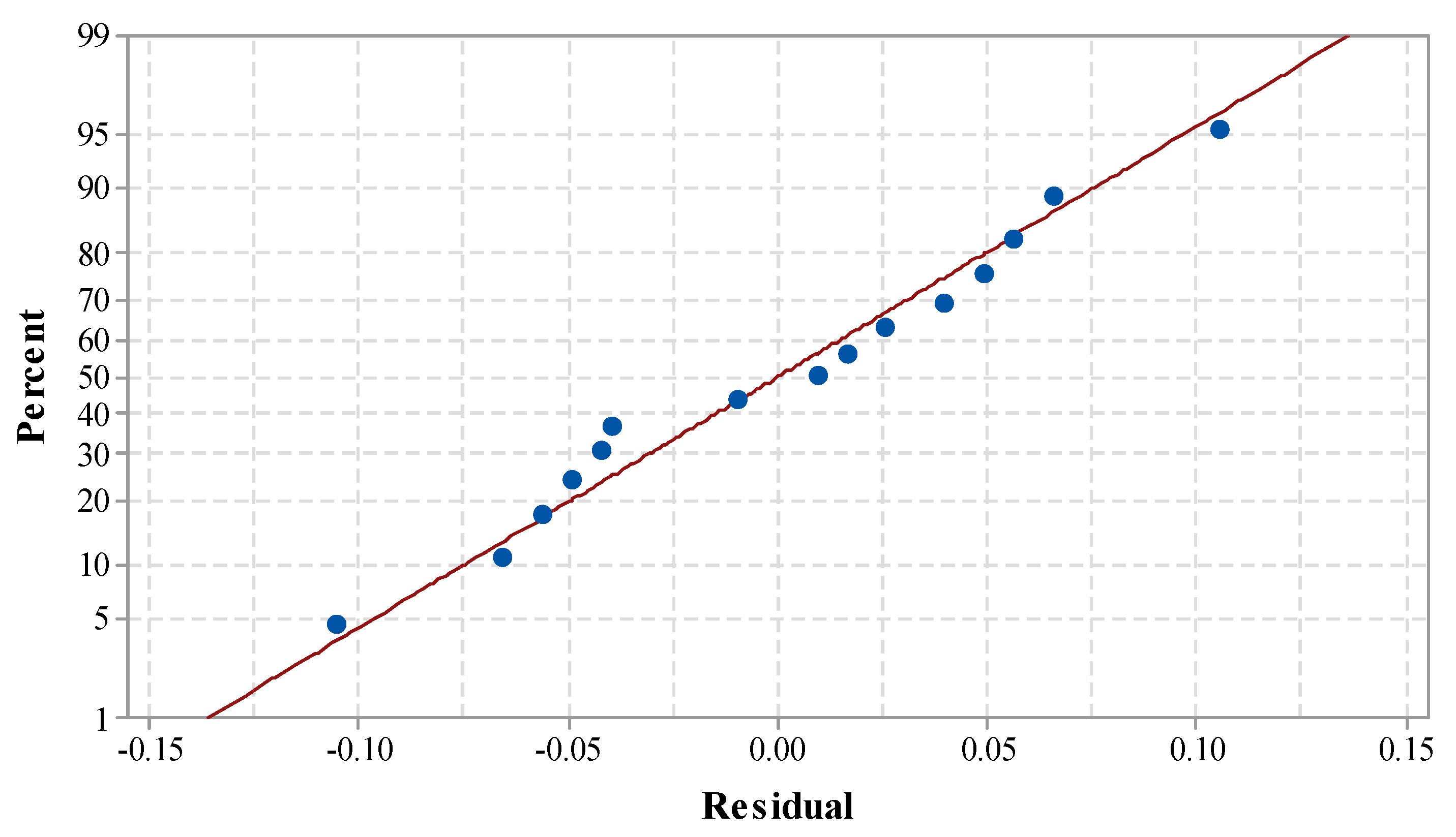
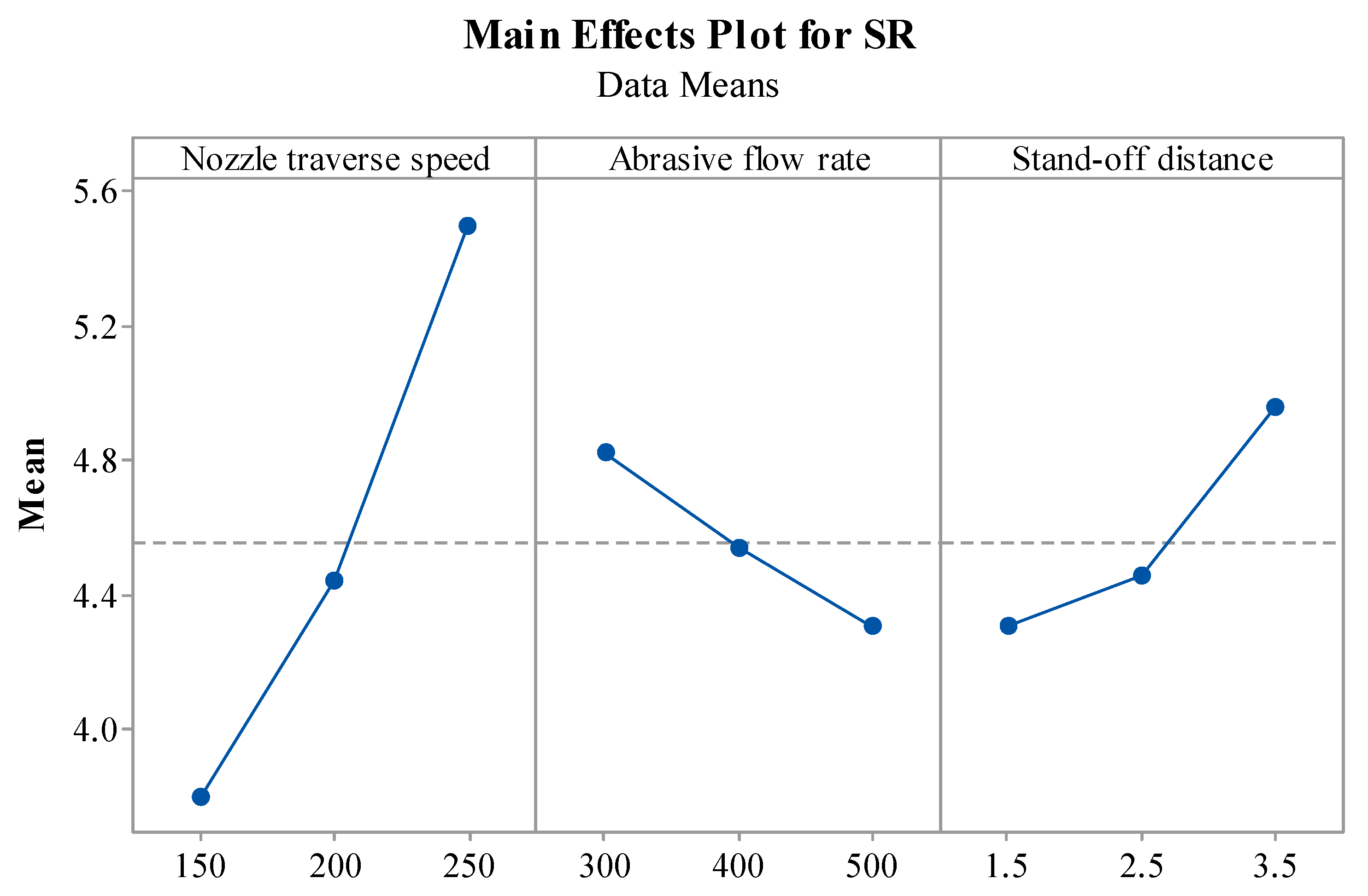
3.2. Analysis of SR
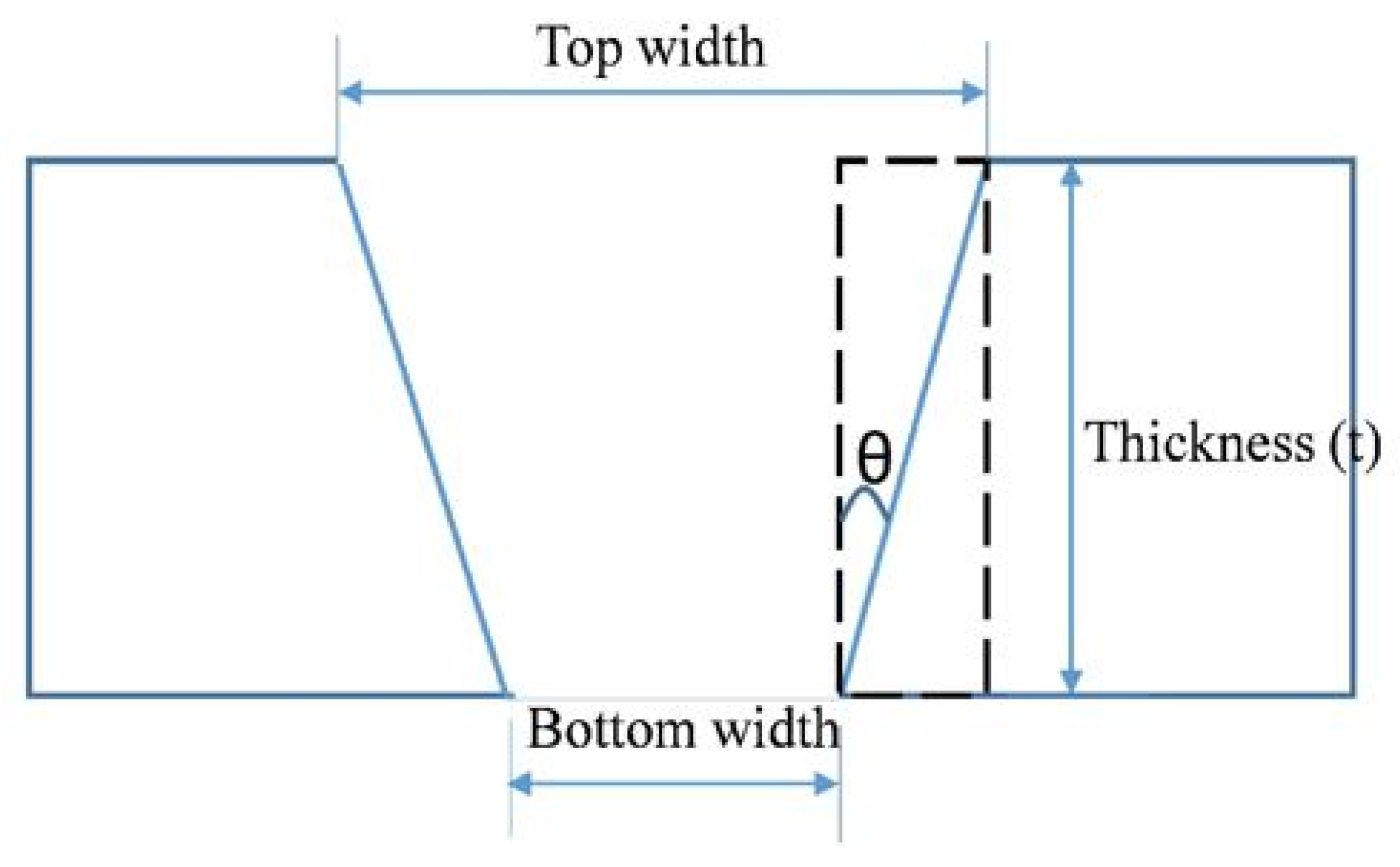
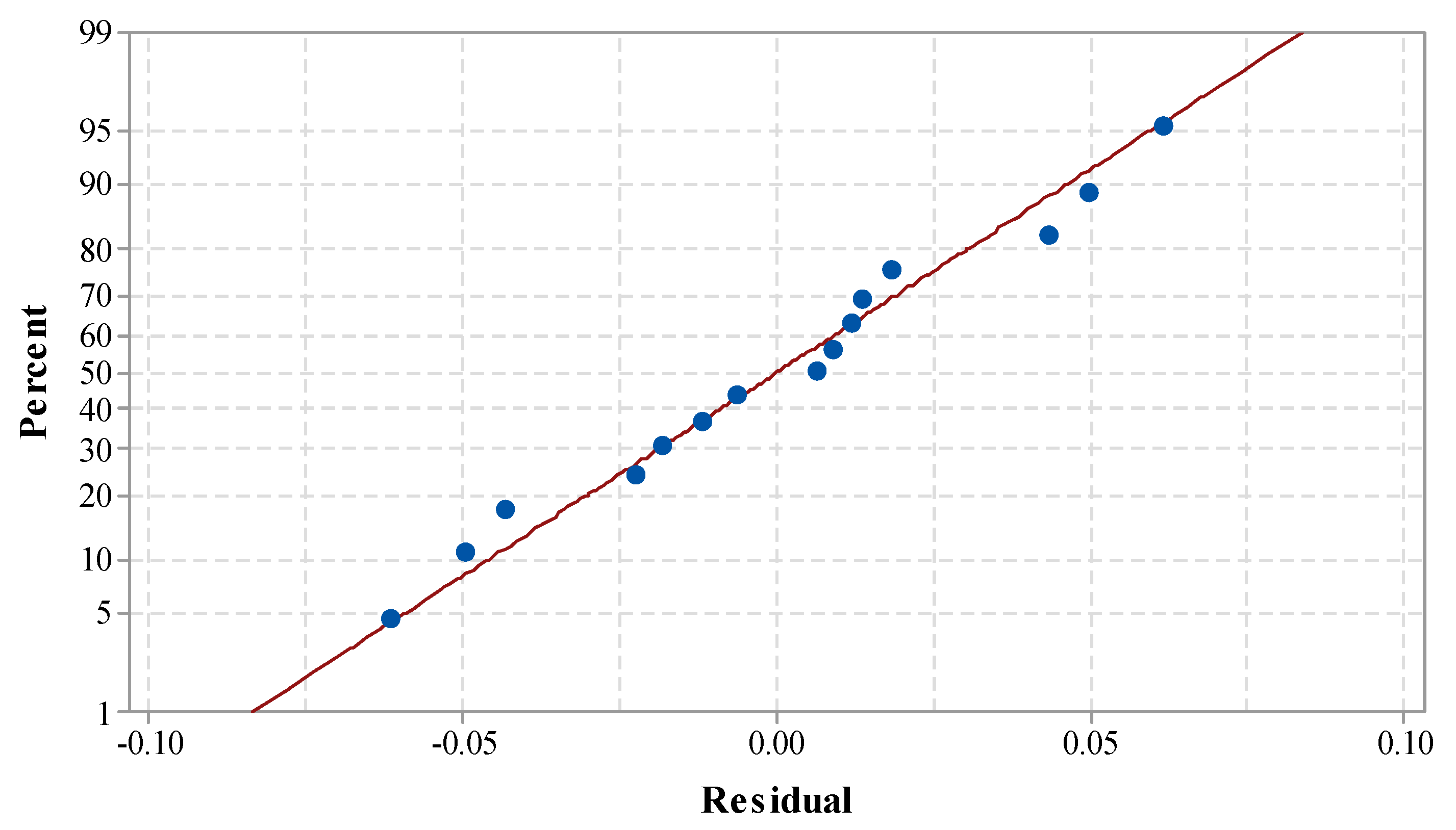
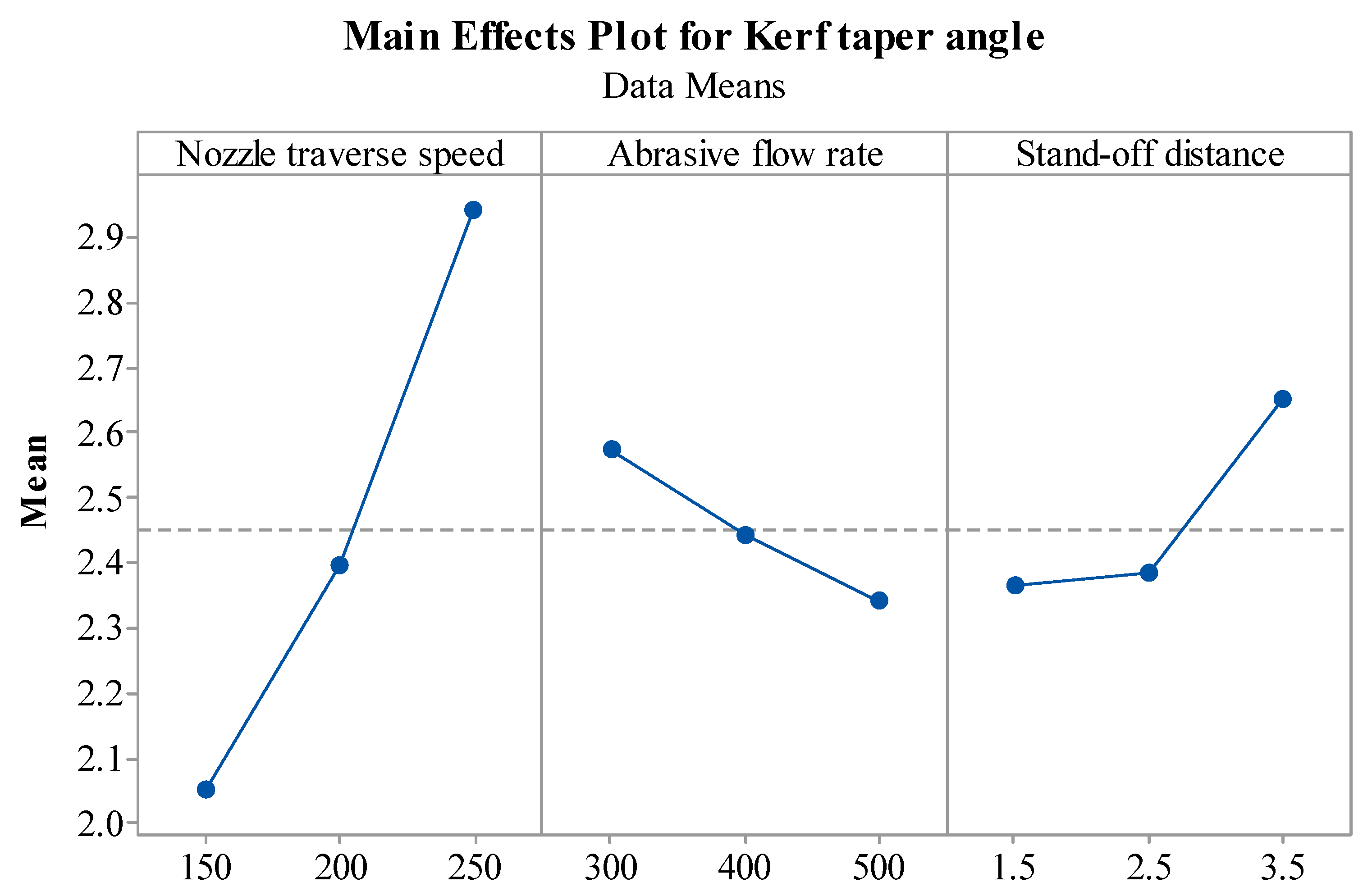
3.3. Analysis of Kerf Taper Angle
3.4. Optimization Using HTS Algorithm
3.4.1. Conduction Phase
3.4.2. Convection Phase
3.4.3. Radiation Phase
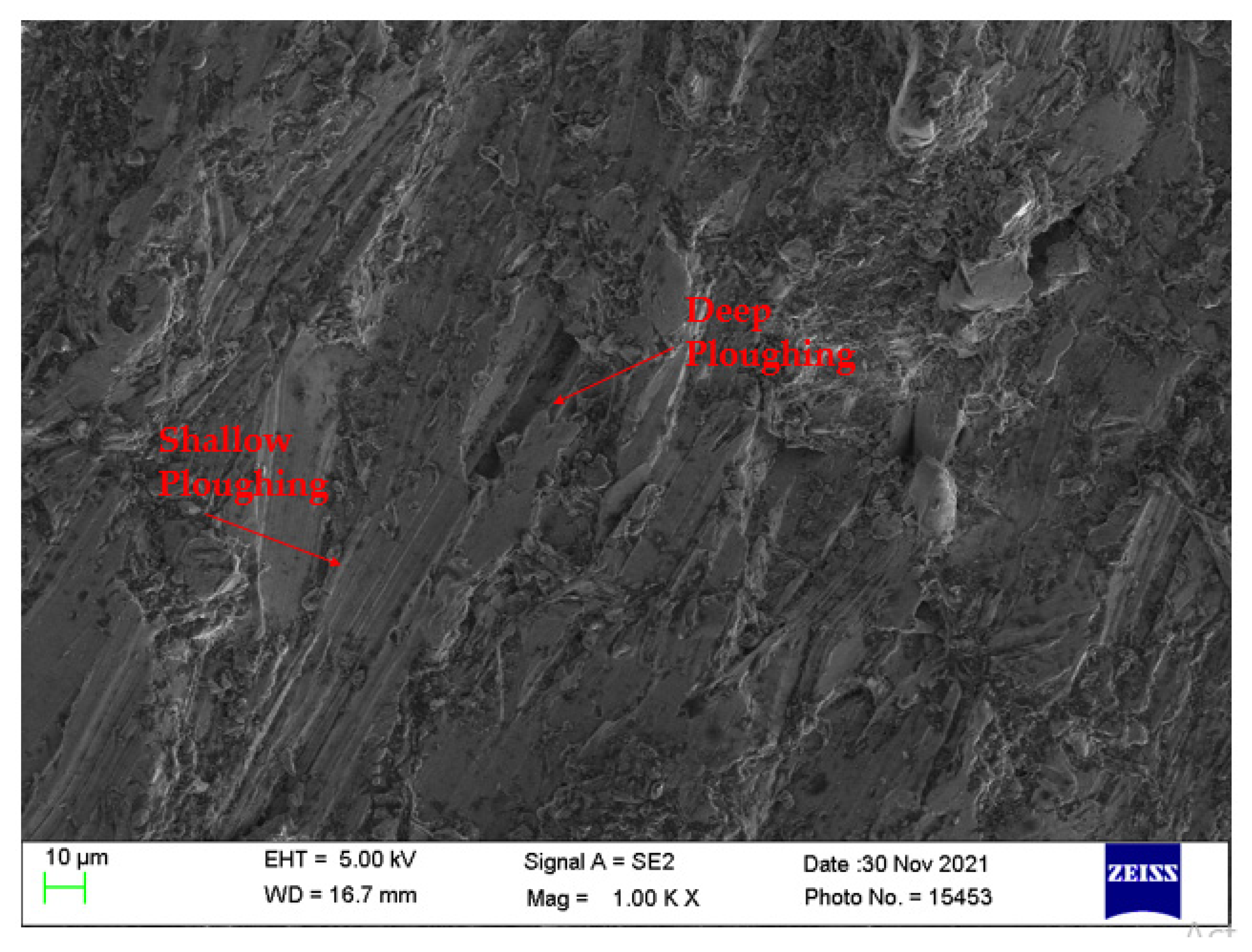
3.5. Surface Morphology of Machined Components
4. Conclusions
- Mathematical regression models were generated using the RSM technique, and ANOVA results have shown the adequacy of the developed models.
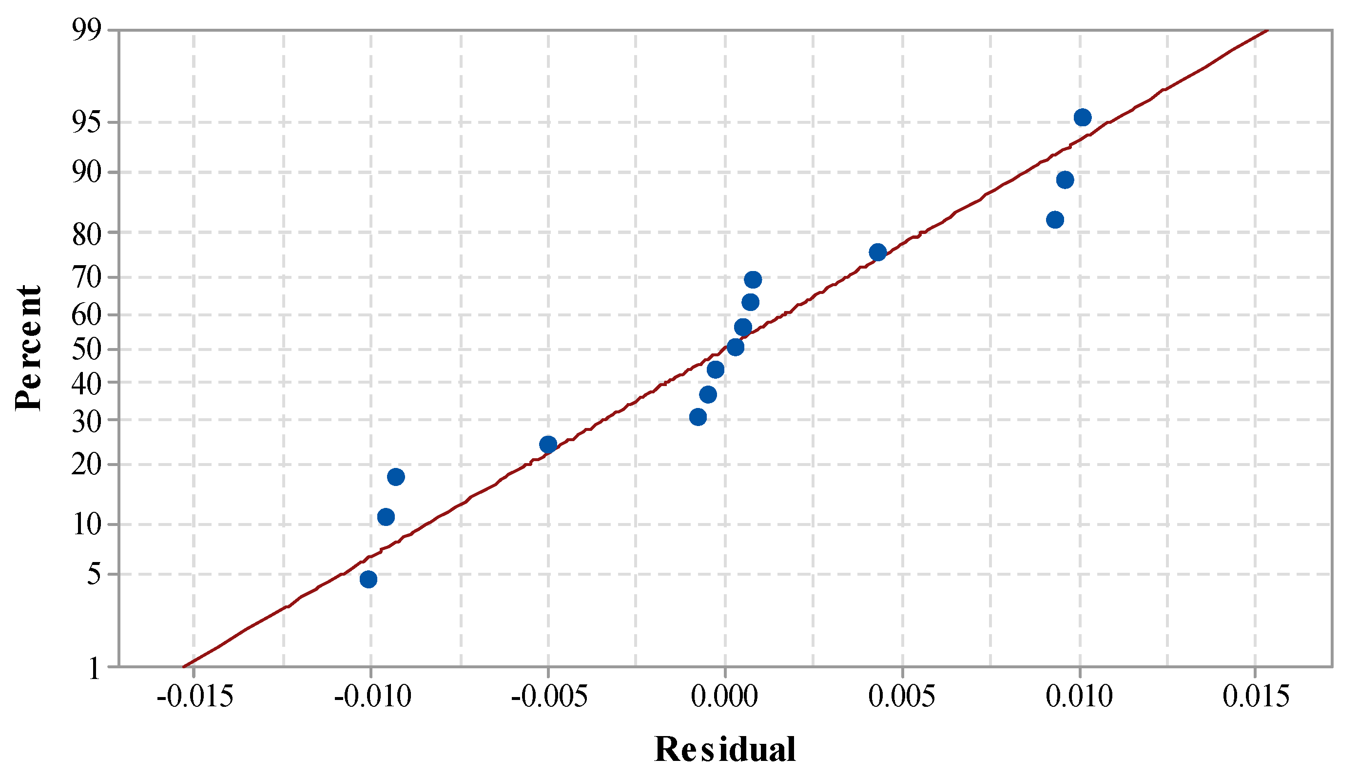
- Normal probability, the significance of model terms, and the insignificance of lack-of-fit for all responses highlighted good prediction capabilities of the developed models of MRR, SR, and the kerf taper angle.
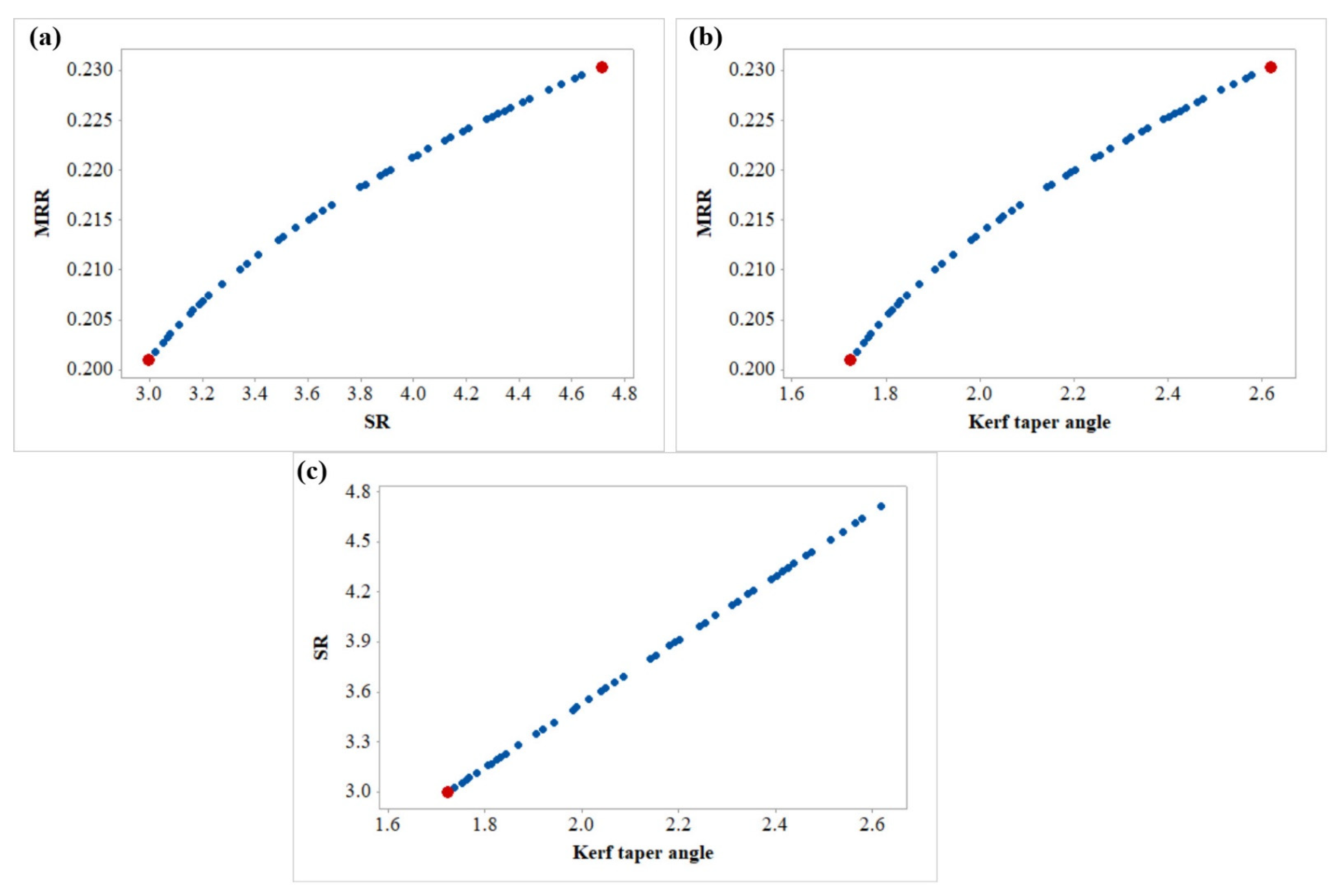
- Single-objective optimization results yielded a maximum MRR of 0.2304 g/min (at Tv of 250 mm/min, Af of 500 g/min, and Sd of 1.5 mm), a minimum SR of 2.99 µm, and a minimum θ of 1.72 (both responses at Tv of 150 mm/min, Af of 500 g/min, and Sd of 1.5 mm). Simultaneous optimization results, by considering an equal weightage of 0.33 to all responses, yielded MRR, SR, and θ values of 0.2133 g/min, 3.50 µm, and 1.98, respectively at Tv of 193 mm/min, Af of 500 g/min, and Sd of 1.5 mm.
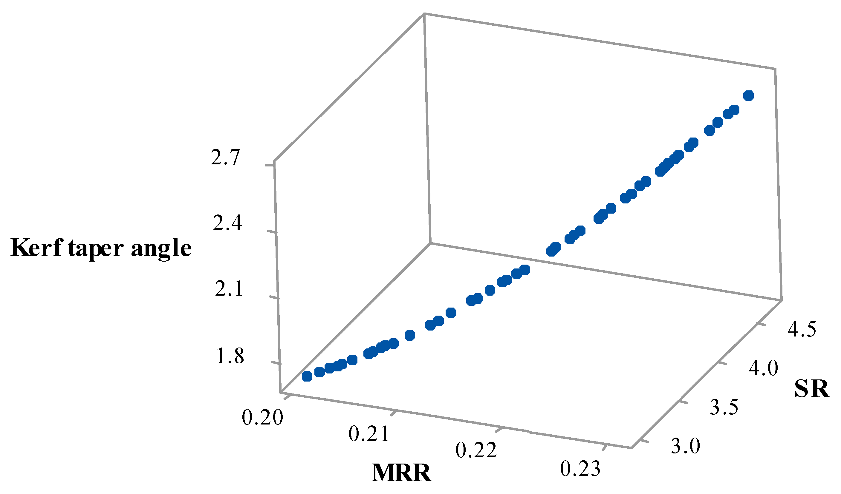
- 3D and 2D plots were plotted using Pareto optimal points, which highlighted the non-dominant feasible solutions. Every single Pareto point gives a unique solution and has a corresponding value of the input process parameter. Therefore, an operator can select a suitable point by just observing their required values of MRR, SR, and the kerf taper angle.
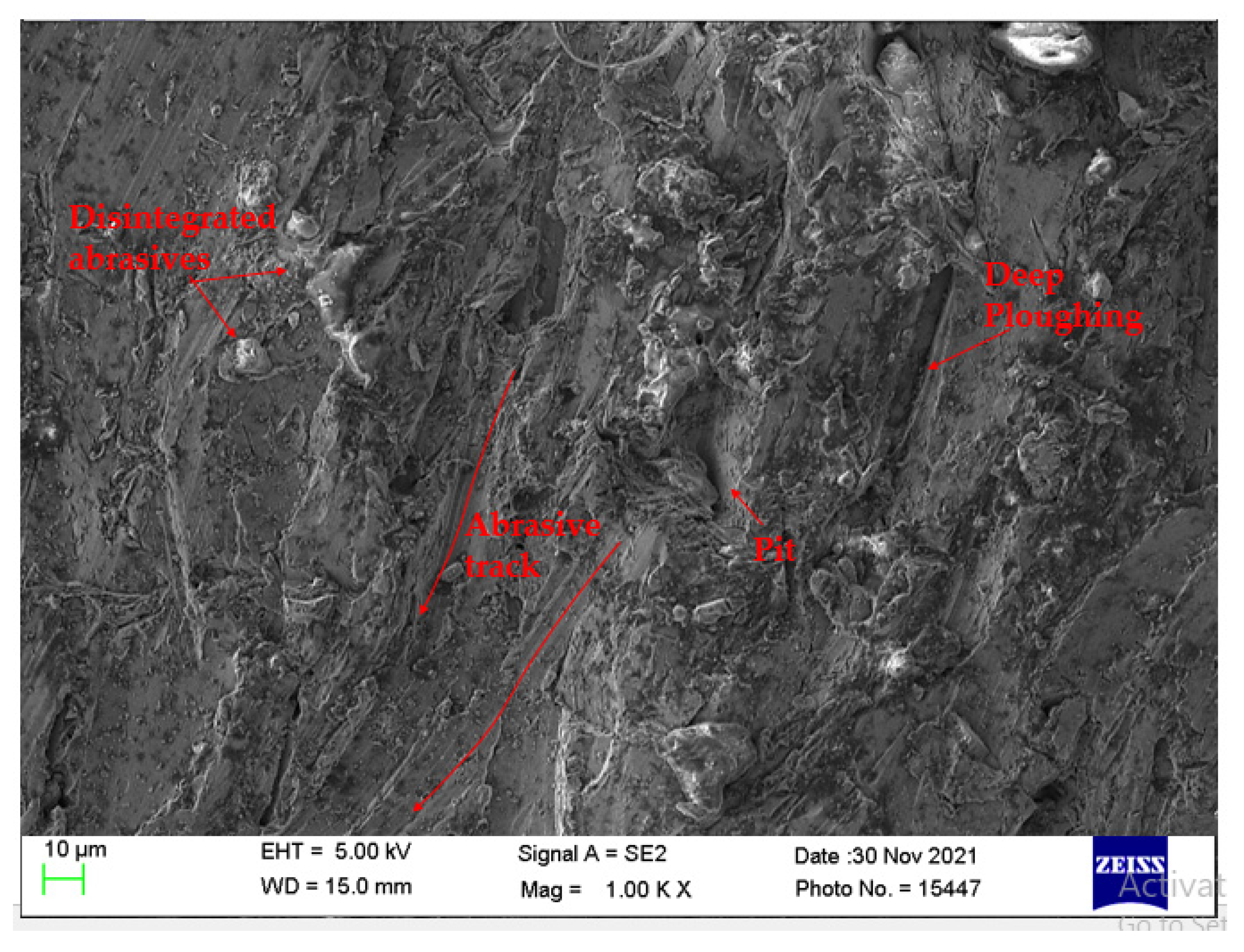
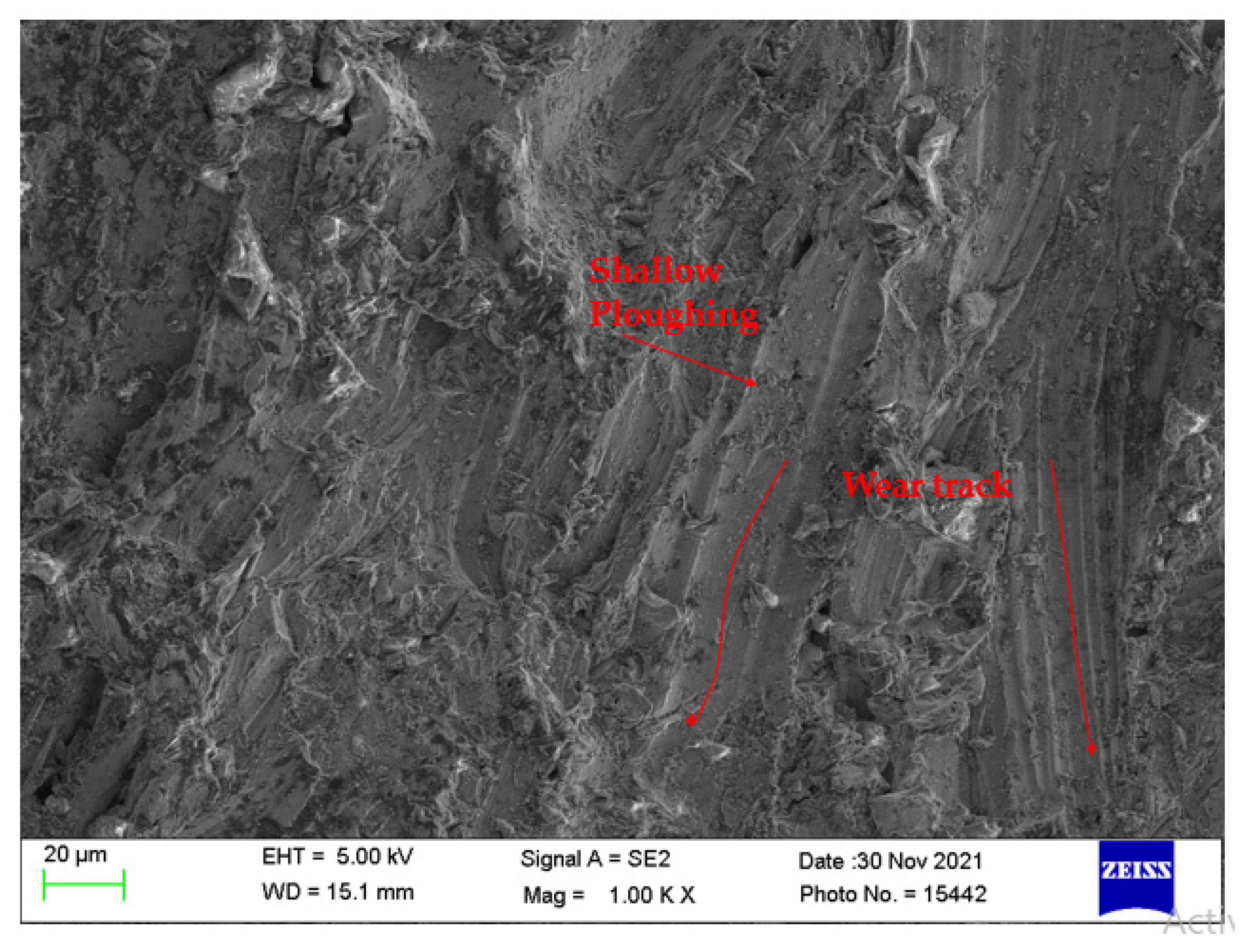
- The surface morphology revealed the material-removal mechanism in AWJM was due to ploughing, particle disintegration, and embedding of fractured abrasive particles in the machined surface.
- Different levels of input process parameters by varying the abrasives can be studied in the future to check the optimal levels of the AWJM responses.
Author Contributions
Funding
Institutional Review Board Statement
Informed Consent Statement
Data Availability Statement
Acknowledgments
Conflicts of Interest
References
- Saravanan, K.; Sudeshkumar, M.; Maridurai, T.; Suyamburajan, V.; Jayaseelan, V. Optimization of SiC Abrasive Parameters on Machining of Ti-6Al-4V Alloy in AJM Using Taguchi-Grey Relational Method. Silicon 2021, 1–8. [Google Scholar] [CrossRef]
- Chaudhari, R.; Vora, J.; Parikh, D.; Wankhede, V.; Khanna, S. Multi-response Optimization of WEDM Parameters Using an Integrated Approach of RSM–GRA Analysis for Pure Titanium. J. Inst. Eng. Series D 2020, 101, 117–126. [Google Scholar] [CrossRef]
- Saini, A.; Pabla, B.; Dhami, S. Developments in cutting tool technology in improving machinability of Ti6Al4V alloy: A review. Proc. Inst. Mech. Eng. Part B J. Eng. Manuf. 2016, 230, 1977–1989. [Google Scholar] [CrossRef]
- Lin, N.; Li, D.; Zou, J.; Xie, R.; Wang, Z.; Tang, B. Surface texture-based surface treatments on Ti6Al4V titanium alloys for tribological and biological applications: A mini review. Materials 2018, 11, 487. [Google Scholar] [CrossRef] [PubMed] [Green Version]
- Nguyen, D.S.; Park, H.S.; Lee, C.M. Optimization of selective laser melting process parameters for Ti-6Al-4V alloy manufacturing using deep learning. J. Manuf. Process. 2020, 55, 230–235. [Google Scholar] [CrossRef]
- Chaturvedi, C.; Rao, P.S.; Khan, M.Y. Optimization of process variable in abrasive water jet Machining (AWJM) of Ti-6Al-4V alloy using Taguchi methodology. Mater. Today Proc. 2021, 47, 6120–6127. [Google Scholar] [CrossRef]
- Khanna, S.; Marathey, P.; Patel, R.; Paneliya, S.; Chaudhari, R.; Vora, J.; Ray, A.; Banerjee, R.; Mukhopadhyay, I. Unravelling camphor mediated synthesis of TiO2 nanorods over shape memory alloy for efficient energy harvesting. Appl. Surf. Sci. 2021, 541, 148489. [Google Scholar] [CrossRef]
- Khan, M.A.; Jaffery, S.H.I.; Khan, M.; Younas, M.; Butt, S.I.; Ahmad, R.; Warsi, S.S. Multi-objective optimization of turning titanium-based alloy Ti-6Al-4V under dry, wet, and cryogenic conditions using gray relational analysis (GRA). Int. J. Adv. Manuf. Technol. 2020, 106, 3897–3911. [Google Scholar] [CrossRef]
- Vora, J.; Chaudhari, R.; Patel, C.; Pimenov, D.Y.; Patel, V.K.; Giasin, K.; Sharma, S. Experimental Investigations and Pareto Optimization of Fiber Laser Cutting Process of Ti6Al4V. Metals 2021, 11, 1461. [Google Scholar] [CrossRef]
- Khanna, S.; Marathey, P.; Paneliya, S.; Chaudhari, R.; Vora, J. Fabrication of rutile–TiO2 nanowire on shape memory alloy: A potential material for energy storage application. Mater. Today Proc. 2021. [Google Scholar] [CrossRef]
- Ishfaq, K.; Asad, M.; Anwar, S.; Pruncu, C.I.; Saleh, M.; Ahmad, S. A comprehensive analysis of the effect of graphene-based dielectric for sustainable electric discharge machining of Ti-6Al-4V. Materials 2021, 14, 23. [Google Scholar] [CrossRef]
- Muthuramalingam, T.; Moiduddin, K.; Akash, R.; Krishnan, S.; Mian, S.H.; Ameen, W.; Alkhalefah, H. Influence of process parameters on dimensional accuracy of machined Titanium (Ti-6Al-4V) alloy in Laser Beam Machining Process. Opt. Laser Technol. 2020, 132, 106494. [Google Scholar] [CrossRef]
- Devarasiddappa, D.; Chandrasekaran, M. Experimental investigation and optimization of sustainable performance measures during wire-cut EDM of Ti-6Al-4V alloy employing preference-based TLBO algorithm. Mater. Manuf. Process. 2020, 35, 1204–1213. [Google Scholar] [CrossRef]
- Karkalos, N.E.; Karmiris-Obratański, P.; Kudelski, R.; Markopoulos, A.P. Experimental Study on the Sustainability Assessment of AWJ Machining of Ti-6Al-4V Using Glass Beads Abrasive Particles. Sustainability 2021, 13, 8917. [Google Scholar] [CrossRef]
- Alberdi, A.; Rivero, A.; López de Lacalle, L. Experimental study of the slot overlapping and tool path variation effect in abrasive waterjet milling. J. Manuf. Sci. Eng. 2011, 133, 034502. [Google Scholar] [CrossRef]
- Natarajan, Y.; Murugesan, P.K.; Mohan, M.; Khan, S.A.L.A. Abrasive Water Jet Machining process: A state of art of review. J. Manuf. Process. 2020, 49, 271–322. [Google Scholar] [CrossRef]
- Saravanan, S.; Vijayan, V.; Suthahar, S.J.; Balan, A.; Sankar, S.; Ravichandran, M. A review on recent progresses in machining methods based on abrasive water jet machining. Mater. Today Proc. 2020, 21, 116–122. [Google Scholar] [CrossRef]
- Thakur, R.; Singh, K. Experimental investigation and optimization of abrasive water jet machining parameter on multi-walled carbon nanotube doped epoxy/carbon laminate. Measurement 2020, 164, 108093. [Google Scholar] [CrossRef]
- Alberdi, A.; Rivero, A.; De Lacalle, L.L.; Etxeberria, I.; Suárez, A. Effect of process parameter on the kerf geometry in abrasive water jet milling. Int. J. Adv. Manuf. Technol. 2010, 51, 467–480. [Google Scholar] [CrossRef]
- Deaconescu, A.; Deaconescu, T. Response Surface Methods Used for Optimization of Abrasive Waterjet Machining of the Stainless Steel X2 CrNiMo 17-12-2. Materials 2021, 14, 2475. [Google Scholar] [CrossRef]
- Tripathi, D.R.; Vachhani, K.H.; Bandhu, D.; Kumari, S.; Kumar, V.R.; Abhishek, K. Experimental investigation and optimization of abrasive waterjet machining parameters for GFRP composites using metaphor-less algorithms. Mater. Manuf. Process. 2021, 36, 803–813. [Google Scholar] [CrossRef]
- Patel, G.M.; Kumar, R.S.; Naidu, N.S. Optimization of abrasive water jet machining for green composites using multi-variant hybrid techniques. In Optimization of Manufacturing Processes; Springer: Berlin/Heidelberg, Germany, 2020; pp. 129–162. [Google Scholar]
- Kumar, K.R.; Sreebalaji, V.; Pridhar, T. Characterization and optimization of abrasive water jet machining parameters of aluminium/tungsten carbide composites. Measurement 2018, 117, 57–66. [Google Scholar] [CrossRef]
- Joel, C.; Joel, L.; Muthukumaran, S.; Shanthini, P.M. Parametric optimization of abrasive water jet machining of C360 brass using MOTLBO. Mater. Today Proc. 2021, 37, 1905–1910. [Google Scholar] [CrossRef]
- Doğankaya, E.; Kahya, M.; Özgür Ünver, H. Abrasive water jet machining of UHMWPE and trade-off optimization. Mater. Manuf. Process. 2020, 35, 1339–1351. [Google Scholar] [CrossRef]
- Reddy, P.V.; Kumar, G.S.; Kumar, V.S. Multi-response Optimization in Machining Inconel-625 by Abrasive Water Jet Machining Process Using WASPAS and MOORA. Arab. J. Sci. Eng. 2020, 45, 9843–9857. [Google Scholar] [CrossRef]
- Samson, R.M.; Rajak, S.; Kannan, T.D.B.; Sampreet, K. Optimization of Process Parameters in Abrasive Water Jet Machining of Inconel 718 Using VIKOR Method. J. Inst. Eng. Series C 2020, 101, 579–585. [Google Scholar] [CrossRef]
- Chaudhari, R.; Vora, J.; Lacalle, L.; Khanna, S.; Patel, V.K.; Ayesta, I. Parametric Optimization and Effect of Nano-Graphene Mixed Dielectric Fluid on Performance of Wire Electrical Discharge Machining Process of Ni55. 8Ti Shape Memory Alloy. Materials 2021, 14, 2533. [Google Scholar] [CrossRef] [PubMed]
- Vora, J.; Patel, V.K.; Srinivasan, S.; Chaudhari, R.; Pimenov, D.Y.; Giasin, K.; Sharma, S. Optimization of Activated Tungsten Inert Gas Welding Process Parameters Using Heat Transfer Search Algorithm: With Experimental Validation Using Case Studies. Metals 2021, 11, 981. [Google Scholar] [CrossRef]
- Chaudhari, R.; Vora, J.J.; Mani Prabu, S.; Palani, I.; Patel, V.K.; Parikh, D.; de Lacalle, L.N.L. Multi-response optimization of WEDM process parameters for machining of superelastic nitinol shape-memory alloy using a heat-transfer search algorithm. Materials 2019, 12, 1277. [Google Scholar] [CrossRef] [Green Version]
- Tawhid, M.A.; Savsani, V. ∊-constraint heat transfer search (∊-HTS) algorithm for solving multi-objective engineering design problems. J. Comput. Des. Eng. 2018, 5, 104–119. [Google Scholar] [CrossRef]
- Chaudhari, R.; Vora, J.J.; Pramanik, A.; Parikh, D. Optimization of Parameters of Spark Erosion Based Processes. In Spark Erosion Machining; CRC Press: Boca Raton, FL, USA, 2020; pp. 190–216. [Google Scholar]
- Patel, V.K.; Raja, B.D. A comparative performance evaluation of the reversed Brayton cycle operated heat pump based on thermo-ecological criteria through many and multi objective approaches. Energy Convers. Manag. 2019, 183, 252–265. [Google Scholar] [CrossRef]
- Raja, B.D.; Jhala, R.; Patel, V. Multiobjective thermo-economic and thermodynamics optimization of a plate–fin heat exchanger. Heat Transf. Asian Res. 2018, 47, 253–270. [Google Scholar] [CrossRef]
- Chaudhari, R.; Vora, J.J.; Prabu, S.M.; Palani, I.; Patel, V.K.; Parikh, D. Pareto optimization of WEDM process parameters for machining a NiTi shape memory alloy using a combined approach of RSM and heat transfer search algorithm. Adv. Manuf. 2021, 9, 64–80. [Google Scholar] [CrossRef]
- Wankhede, V.; Jagetiya, D.; Joshi, A.; Chaudhari, R. Experimental investigation of FDM process parameters using Taguchi analysis. Mater. Today Proc. 2020, 27, 2117–2120. [Google Scholar] [CrossRef]
- Chaurasia, A.; Wankhede, V.; Chaudhari, R. Experimental investigation of high-speed turning of INCONEL 718 using PVD-coated carbide tool under wet condition. In Innovations in Infrastructure; Springer: Berlin/Heidelberg, Germany, 2019; pp. 367–374. [Google Scholar]
- Sheth, M.; Gajjar, K.; Jain, A.; Shah, V.; Patel, H.; Chaudhari, R.; Vora, J. Multi-objective optimization of inconel 718 using Combined approach of taguchi—Grey relational analysis. In Advances in Mechanical Engineering; Springer: Berlin/Heidelberg, Germany, 2021; pp. 229–235. [Google Scholar]
- Rathi, P.; Ghiya, R.; Shah, H.; Srivastava, P.; Patel, S.; Chaudhari, R.; Vora, J. Multi-response Optimization of Ni55. 8Ti Shape Memory Alloy Using Taguchi–Grey Relational Analysis Approach. In Recent Advances in Mechanical Infrastructure; Springer: Berlin/Heidelberg, Germany, 2020; pp. 13–23. [Google Scholar]
- Dzionk, S.; Siemiątkowski, M.S. Studying the effect of working conditions on WEDM machining performance of super alloy Inconel 617. Machines 2020, 8, 54. [Google Scholar] [CrossRef]
- Vishwakarma, M.; Parashar, V.; Khare, V. Regression analysis and optimization of material removal rate on electric discharge machine for EN-19 alloy steel. Int. J. Sci. Res. Publ. 2012, 2, 145–153. [Google Scholar]
- Tiwari, T.; Sourabh, S.; Nag, A.; Dixit, A.R.; Mandal, A.; Das, A.K.; Mandal, N.; Srivastava, A.K. Parametric investigation on abrasive waterjet machining of alumina ceramic using response surface methodology. In Proceedings of the IOP Conference Series: Materials Science and Engineering; IOP Publishing: Bristol, UK, 2018; p. 012005. [Google Scholar]
- Chaudhari, R.; Khanna, S.; Vora, J.; Patel, V.K.; Paneliya, S.; Pimenov, D.Y.; Giasin, K.; Wojciechowski, S. Experimental investigations and optimization of MWCNTs-mixed WEDM process parameters of nitinol shape memory alloy. J. Mater. Res. Technol. 2021, 15, 2152–2169. [Google Scholar] [CrossRef]
- Bhowmik, S.; Ray, A. Abrasive water jet machining of composite materials. In Advanced Manufacturing Technologies; Springer: Berlin/Heidelberg, Germany, 2017; pp. 77–97. [Google Scholar]
- Reddy, D.S.; Kumar, A.S.; Rao, M.S. Parametric optimization of abrasive water jet machining of Inconel 800H using Taguchi methodology. Univers. J. Mech. Eng. 2014, 2, 158–162. [Google Scholar] [CrossRef]
- Dumbhare, P.A.; Dubey, S.; Deshpande, Y.V.; Andhare, A.B.; Barve, P.S. Modelling and multi-objective optimization of surface roughness and kerf taper angle in abrasive water jet machining of steel. J. Braz. Soc. Mech. Sci. Eng. 2018, 40, 259. [Google Scholar] [CrossRef]
- Patel, V.K.; Savsani, V.J. Heat transfer search (HTS): A novel optimization algorithm. Inf. Sci. 2015, 324, 217–246. [Google Scholar] [CrossRef]
- Kumar, S.; Tejani, G.G.; Pholdee, N.; Bureerat, S. Multi-objective modified heat transfer search for truss optimization. Eng. Comput. 2021, 37, 3439–3454. [Google Scholar] [CrossRef]
- Chaudhari, R.; Vora, J.J.; Patel, V.; Lacalle, L.; Parikh, D. Effect of WEDM process parameters on surface morphology of nitinol shape memory alloy. Materials 2020, 13, 4943. [Google Scholar] [CrossRef] [PubMed]
- Tejani, G.G.; Kumar, S.; Gandomi, A.H. Multi-objective heat transfer search algorithm for truss optimization. Eng. Comput. 2021, 37, 641–662. [Google Scholar] [CrossRef]
- Kumar, S.; Tejani, G.G.; Pholdee, N.; Bureerat, S. Multi-Objective Passing Vehicle Search algorithm for structure optimization. Expert Syst. Appl. 2021, 169, 114511. [Google Scholar] [CrossRef]
- Chaudhari, R.; Vora, J.J.; Patel, V.; López de Lacalle, L.; Parikh, D. Surface analysis of wire-electrical-discharge-machining-processed shape-memory alloys. Materials 2020, 13, 530. [Google Scholar] [CrossRef] [Green Version]
- Yuvaraj, N.; Kumar, M.P. Investigation of process parameters influence in abrasive water jet cutting of D2 steel. Mater. Manuf. Process. 2017, 32, 151–161. [Google Scholar] [CrossRef]
- Rajadurai, A. Experimental study on deep-hole making in Ti-6Al-4V by abrasive water jet machining. Mater. Res. Express 2019, 6, 066532. [Google Scholar]
- Hascalik, A.; Çaydaş, U.; Gürün, H. Effect of traverse speed on abrasive waterjet machining of Ti–6Al–4V alloy. Mater. Des. 2007, 28, 1953–1957. [Google Scholar] [CrossRef]


| C | Fe | Al | N2 | Cu | V | Ti |
|---|---|---|---|---|---|---|
| 0.05 | 0.20 | 6.20 | 0.04 | 0.001 | 4.0 | Balanced |
| Process Parameter | Level (−1) | Level (0) | Level (1) |
|---|---|---|---|
| Nozze Transverse Speed (Tv), mm/min | 150 | 200 | 250 |
| Abrasive Flow Rate (Af), g/min | 300 | 400 | 500 |
| Stand-off distance (Sd), mm | 1.5 | 2.5 | 3.5 |
| Mesh size of abrasive | 80 | ||
| Nozzle material | ROCTEC 100 Composite Carbide | ||
| Nozzle diameter | 1.02 mm | ||
| Orifice material/diameter | Diamond/0.33 mm | ||
| Impact angle of jet | 90° | ||
| Standard Order | Run Order | Tv (mm/min) | Af (g/min) | Sd (mm) | MRR (g/min) | SR (µm) | θ (°) |
|---|---|---|---|---|---|---|---|
| 8 | 1 | 250 | 400 | 3.5 | 0.1767 | 5.73 | 3.06 |
| 15 | 2 | 200 | 400 | 2.5 | 0.1706 | 4.32 | 2.31 |
| 4 | 3 | 250 | 500 | 2.5 | 0.2062 | 5.27 | 2.82 |
| 10 | 4 | 200 | 500 | 1.5 | 0.2250 | 3.58 | 2.06 |
| 12 | 5 | 200 | 500 | 3.5 | 0.2062 | 4.99 | 2.67 |
| 9 | 6 | 200 | 300 | 1.5 | 0.1076 | 4.76 | 2.53 |
| 11 | 7 | 200 | 300 | 3.5 | 0.1302 | 4.87 | 2.60 |
| 13 | 8 | 200 | 400 | 2.5 | 0.1650 | 4.26 | 2.28 |
| 6 | 9 | 250 | 400 | 1.5 | 0.1768 | 5.31 | 2.86 |
| 5 | 10 | 150 | 400 | 1.5 | 0.1375 | 3.59 | 2.007 |
| 1 | 11 | 150 | 300 | 2.5 | 0.1302 | 3.96 | 2.12 |
| 2 | 12 | 250 | 300 | 2.5 | 0.1303 | 5.68 | 3.04 |
| 3 | 13 | 150 | 500 | 2.5 | 0.2063 | 3.39 | 2.11 |
| 7 | 14 | 150 | 400 | 3.5 | 0.1768 | 4.24 | 2.27 |
| 14 | 15 | 200 | 400 | 2.5 | 0.1743 | 4.33 | 2.31 |
| Source | DF | Adj SS | Adj MS | F Value | p-Value | Significance |
|---|---|---|---|---|---|---|
| Model | 5 | 0.016149 | 0.003230 | 46.42 | 0.000 | Significant |
| Linear | 3 | 0.008332 | 0.002777 | 39.92 | 0.000 | Significant |
| Tv | 1 | 0.000514 | 0.000514 | 7.39 | 0.024 | Significant |
| Af | 1 | 0.002825 | 0.002825 | 40.61 | 0.000 | Significant |
| Sd | 1 | 0.000912 | 0.000912 | 13.11 | 0.006 | Significant |
| 2-way interaction | 2 | 0.000814 | 0.000407 | 5.85 | 0.024 | Significant |
| Tv Sd | 1 | 0.000386 | 0.000386 | 5.55 | 0.043 | Significant |
| Af Sd | 1 | 0.000429 | 0.000429 | 6.16 | 0.035 | Significant |
| Error | 9 | 0.000626 | 0.000070 | |||
| Lack of Fit | 7 | 0.000582 | 0.000083 | 3.79 | 0.225 | Insignificant |
| Pure Error | 2 | 0.000044 | 0.000022 | |||
| Total | 14 | 0.016775 | ||||
| S = 0.008341, R-Sq. = 96.27%, R-Sq. (Adj.) = 94.19% | ||||||
| Source | DF | Adj SS | Adj MS | F Value | p-Value | Significance |
|---|---|---|---|---|---|---|
| Model | 6 | 7.86108 | 1.31018 | 133.17 | 0.000 | Significant |
| Linear | 3 | 0.74036 | 0.24679 | 25.08 | 0.000 | Significant |
| Tv | 1 | 0.04482 | 0.04482 | 4.56 | 0.065 | Significant |
| Af | 1 | 0.68120 | 0.68120 | 69.24 | 0.000 | Significant |
| Sd | 1 | 0.34918 | 0.34918 | 35.49 | 0.000 | Significant |
| Square | 2 | 0.29148 | 0.14574 | 14.81 | 0.002 | Significant |
| Tv Tv | 1 | 0.17409 | 0.17409 | 17.69 | 0.003 | Significant |
| Sd Sd | 1 | 0.13805 | 0.13805 | 14.03 | 0.006 | Significant |
| 2-way interaction | 1 | 0.42739 | 0.42739 | 43.44 | 0.000 | Significant |
| Af Sd | 1 | 0.42739 | 0.42739 | 43.44 | 0.000 | Significant |
| Error | 8 | 0.07871 | 0.00984 | |||
| Lack of Fit | 6 | 0.07599 | 0.01266 | 9.32 | 0.100 | Insignificant |
| Pure Error | 2 | 0.00272 | 0.00136 | |||
| Total | 14 | 7.93978 | ||||
| S = 0.0991, R-Sq. = 99.01%, R-Sq. (Adj.) = 98.27% | ||||||
| Source | DF | Adj SS | Adj MS | F Value | p-Value | Significance |
|---|---|---|---|---|---|---|
| Model | 6 | 2.04354 | 0.34059 | 111.22 | 0.000 | Significant |
| Linear | 3 | 0.15244 | 0.05081 | 16.59 | 0.001 | Significant |
| Tv | 1 | 0.01183 | 0.01183 | 3.86 | 0.085 | Insignificant |
| Af | 1 | 0.12179 | 0.12179 | 39.77 | 0.000 | Significant |
| Sd | 1 | 0.10307 | 0.10307 | 33.66 | 0.000 | Significant |
| Square | 2 | 0.10476 | 0.05238 | 17.11 | 0.001 | Significant |
| Tv Tv | 1 | 0.04692 | 0.04692 | 15.32 | 0.004 | Significant |
| Sd Sd | 1 | 0.06521 | 0.06521 | 21.29 | 0.002 | Significant |
| 2-way interaction | 1 | 0.07268 | 0.07268 | 23.73 | 0.001 | Significant |
| Af Sd | 1 | 0.07268 | 0.07268 | 23.73 | 0.001 | Significant |
| Error | 8 | 0.02450 | 0.00306 | |||
| Lack of Fit | 6 | 0.02372 | 0.00395 | 10.18 | 0.092 | Insignificant |
| Pure Error | 2 | 0.00078 | 0.00038 | |||
| Total | 14 | 2.06804 | ||||
| S = 0.0553, R-Sq. = 98.82%, R-Sq. (Adj.) = 97.93% | ||||||
| Objective Function | Tv (mm/min) | Af (g/min) | Sd (mm) | MRR (g/min) | SR (µm) | θ (°) |
|---|---|---|---|---|---|---|
| Maximum MRR | 250 | 500 | 1.5 | 0.2304 | 4.71 | 2.61 |
| Minimum SR | 150 | 500 | 1.5 | 0.2009 | 2.99 | 1.72 |
| Minimum θ | 150 | 500 | 1.5 | 0.2009 | 2.99 | 1.72 |
| Sr. No. | Tv (mm/min) | Af (g/min) | Sd (mm) | MRR (g/min) | SR (µm) | θ (°) |
|---|---|---|---|---|---|---|
| 1 | 250 | 500 | 1.5 | 0.2304 | 4.71 | 2.62 |
| 2 | 150 | 500 | 1.5 | 0.2009 | 3.00 | 1.72 |
| 3 | 219 | 500 | 1.5 | 0.2213 | 3.99 | 2.24 |
| 4 | 215 | 500 | 1.5 | 0.2201 | 3.91 | 2.20 |
| 5 | 247 | 500 | 1.5 | 0.2295 | 4.64 | 2.58 |
| 6 | 162 | 500 | 1.5 | 0.2044 | 3.11 | 1.78 |
| 7 | 232 | 500 | 1.5 | 0.2251 | 4.28 | 2.39 |
| 8 | 225 | 500 | 1.5 | 0.2230 | 4.12 | 2.31 |
| 9 | 222 | 500 | 1.5 | 0.2221 | 4.06 | 2.28 |
| 10 | 198 | 500 | 1.5 | 0.2151 | 3.60 | 2.04 |
| 11 | 195 | 500 | 1.5 | 0.2142 | 3.55 | 2.02 |
| 12 | 166 | 500 | 1.5 | 0.2056 | 3.15 | 1.81 |
| 13 | 228 | 500 | 1.5 | 0.2239 | 4.19 | 2.34 |
| 14 | 226 | 500 | 1.5 | 0.2233 | 4.14 | 2.32 |
| 15 | 156 | 500 | 1.5 | 0.2027 | 3.05 | 1.75 |
| 16 | 176 | 500 | 1.5 | 0.2086 | 3.28 | 1.87 |
| 17 | 172 | 500 | 1.5 | 0.2074 | 3.22 | 1.84 |
| 18 | 201 | 500 | 1.5 | 0.2159 | 3.65 | 2.07 |
| 19 | 229 | 500 | 1.5 | 0.2242 | 4.21 | 2.36 |
| 20 | 159 | 500 | 1.5 | 0.2036 | 3.08 | 1.77 |
| 21 | 153 | 500 | 1.5 | 0.2018 | 3.02 | 1.74 |
| 22 | 246 | 500 | 1.5 | 0.2292 | 4.61 | 2.57 |
| 23 | 181 | 500 | 1.5 | 0.2100 | 3.34 | 1.91 |
| 24 | 244 | 500 | 1.5 | 0.2286 | 4.56 | 2.54 |
| 25 | 242 | 500 | 1.5 | 0.2280 | 4.51 | 2.51 |
| 26 | 239 | 500 | 1.5 | 0.2272 | 4.44 | 2.48 |
| 27 | 238 | 500 | 1.5 | 0.2269 | 4.41 | 2.46 |
| 28 | 236 | 500 | 1.5 | 0.2263 | 4.37 | 2.44 |
| 29 | 235 | 500 | 1.5 | 0.2260 | 4.34 | 2.43 |
| 30 | 234 | 500 | 1.5 | 0.2257 | 4.32 | 2.41 |
| 31 | 233 | 500 | 1.5 | 0.2254 | 4.30 | 2.40 |
| 32 | 170 | 500 | 1.5 | 0.2068 | 3.20 | 1.83 |
| 33 | 169 | 500 | 1.5 | 0.2065 | 3.19 | 1.82 |
| 34 | 167 | 500 | 1.5 | 0.2059 | 3.17 | 1.81 |
| 35 | 220 | 500 | 1.5 | 0.2216 | 4.02 | 2.26 |
| 36 | 214 | 500 | 1.5 | 0.2198 | 3.89 | 2.19 |
| 37 | 213 | 500 | 1.5 | 0.2195 | 3.87 | 2.18 |
| 38 | 158 | 500 | 1.5 | 0.2033 | 3.07 | 1.76 |
| 39 | 210 | 500 | 1.5 | 0.2186 | 3.82 | 2.15 |
| 40 | 209 | 500 | 1.5 | 0.2183 | 3.80 | 2.14 |
| 41 | 203 | 500 | 1.5 | 0.2165 | 3.69 | 2.09 |
| 42 | 203 | 500 | 1.5 | 0.2165 | 3.69 | 2.09 |
| 43 | 186 | 500 | 1.5 | 0.2115 | 3.41 | 1.94 |
| 44 | 183 | 500 | 1.5 | 0.2106 | 3.37 | 1.92 |
| 45 | 199 | 500 | 1.5 | 0.2154 | 3.62 | 2.05 |
| 46 | 192 | 500 | 1.5 | 0.2133 | 3.51 | 1.99 |
| 47 | 191 | 500 | 1.5 | 0.2130 | 3.49 | 1.98 |
| 48 | 229 | 500 | 1.5 | 0.2242 | 4.21 | 2.36 |
| Sr. No. | Tv (mm/min) | Af (g/min) | Sd (mm) | Predicted Values by HTS Algorithm | Experimentally Measured Values | % Deviation | ||||||
|---|---|---|---|---|---|---|---|---|---|---|---|---|
| MRR | SR | θ | MRR | SR | θ | MRR | SR | θ | ||||
| 1 | 250 | 500 | 1.5 | 0.2304 | 4.71 | 2.61 | 0.2395 | 4.57 | 2.52 | 3.79 | 3.06 | 3.57 |
| 2 | 150 | 500 | 1.5 | 0.2009 | 2.99 | 1.72 | 0.2101 | 2.83 | 1.78 | 4.37 | 5.65 | 3.37 |
| 10 | 192 | 500 | 1.5 | 0.2133 | 3.50 | 1.98 | 0.2194 | 3.69 | 2.06 | 2.78 | 5.14 | 3.88 |
| 38 | 158 | 500 | 1.5 | 0.2033 | 3.07 | 1.76 | 0.1997 | 3.15 | 1.84 | 1.80 | 2.53 | 4.34 |
Publisher’s Note: MDPI stays neutral with regard to jurisdictional claims in published maps and institutional affiliations. |
© 2021 by the authors. Licensee MDPI, Basel, Switzerland. This article is an open access article distributed under the terms and conditions of the Creative Commons Attribution (CC BY) license (https://creativecommons.org/licenses/by/4.0/).
Share and Cite
Fuse, K.; Chaudhari, R.; Vora, J.; Patel, V.K.; de Lacalle, L.N.L. Multi-Response Optimization of Abrasive Waterjet Machining of Ti6Al4V Using Integrated Approach of Utilized Heat Transfer Search Algorithm and RSM. Materials 2021, 14, 7746. https://0-doi-org.brum.beds.ac.uk/10.3390/ma14247746
Fuse K, Chaudhari R, Vora J, Patel VK, de Lacalle LNL. Multi-Response Optimization of Abrasive Waterjet Machining of Ti6Al4V Using Integrated Approach of Utilized Heat Transfer Search Algorithm and RSM. Materials. 2021; 14(24):7746. https://0-doi-org.brum.beds.ac.uk/10.3390/ma14247746
Chicago/Turabian StyleFuse, Kishan, Rakesh Chaudhari, Jay Vora, Vivek K. Patel, and Luis Norberto Lopez de Lacalle. 2021. "Multi-Response Optimization of Abrasive Waterjet Machining of Ti6Al4V Using Integrated Approach of Utilized Heat Transfer Search Algorithm and RSM" Materials 14, no. 24: 7746. https://0-doi-org.brum.beds.ac.uk/10.3390/ma14247746