Description of the Microstructure Development Model Modification
In the literature [
24,
25,
26,
27,
28,
29,
30], one can encounter two-step curves describing the growth of the fraction of the softened structure as a function of the thermodynamic conditions of the forming process, i.e., temperature, strain, strain rate and grain size, during the interpass time. The most complete data set represents the work of authors around Medina [
27,
28,
29,
30,
31,
32,
33,
34,
35,
36,
37]. The data of these authors were used in the modification of our model.
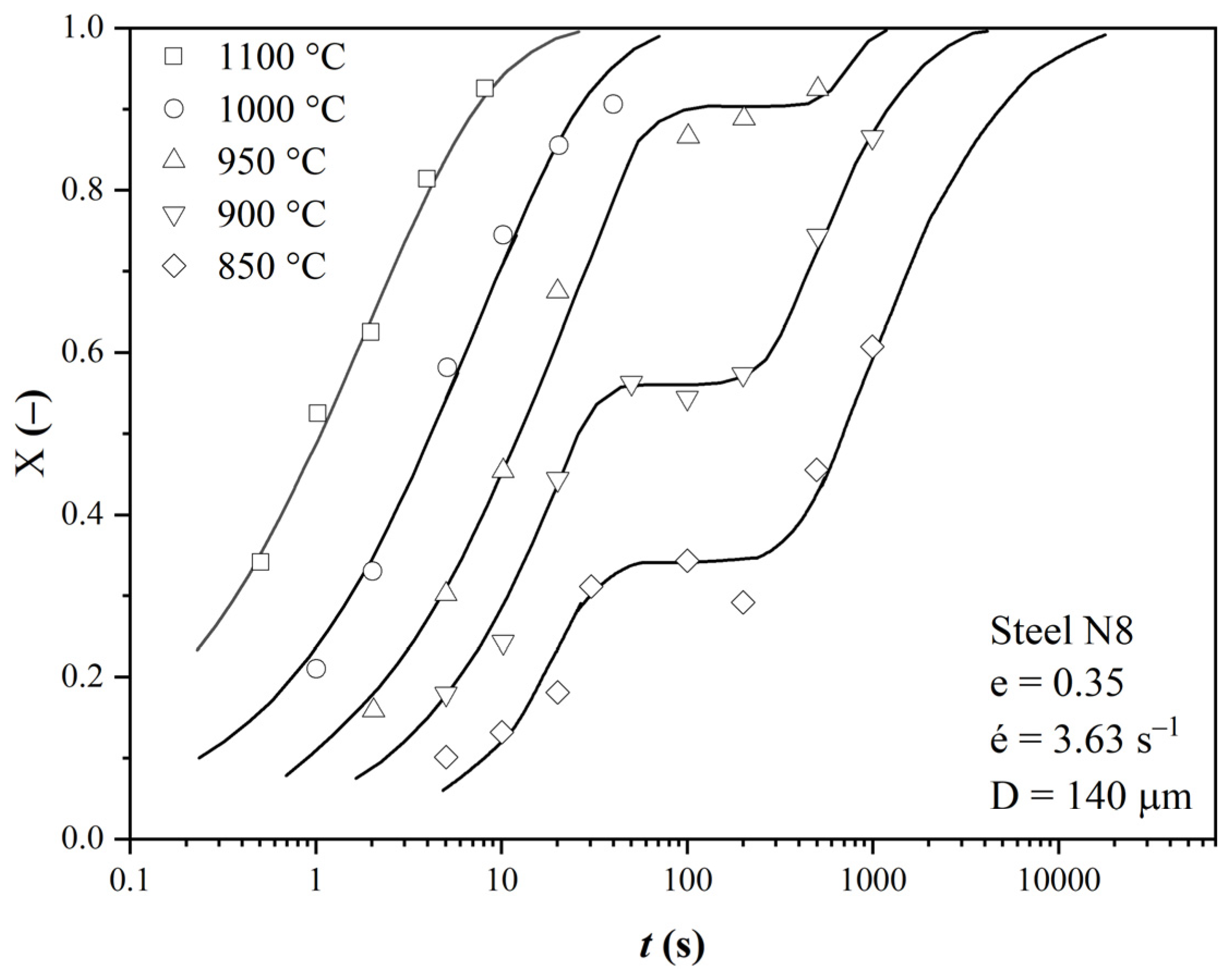
Figure 1 is an example of the two-stage softening curves [
37] for steel, with the chemical composition listed in
Table 1 for N8 steel.
These curves generally determine the time to soften half of the structure, t0.5, that occurs in the JMAK equation. This is the imaginary intersection of the value of X = 0.5 with these curves. In the case of simple S-curves, this is their inflection point. In the case of two-degree curves, this rule no longer applies. The values of t0.5 thus obtained are used to develop an equation that respects the effect of precipitation on the kinetics of recrystallization. The disadvantage, however, is that the equation thus developed leads to a shift of t0.5 to high times in cases where the conditions for initiating strain-induced precipitation (SIP) have not yet been fulfilled during the previous rolling. Moreover, in the temperature region of the nose of the curve of the onset of precipitation, the values of t0.5 in the equations thus developed are biased because they do not consider the step effect of the precipitation on the kinetics of recrystallization. We attempted to use published data for steels N3, N4 and N8 to develop new equations to calculate t0.5 separately for the situation in which SIP takes place and separately for the situation in which SIP does not occur at all.
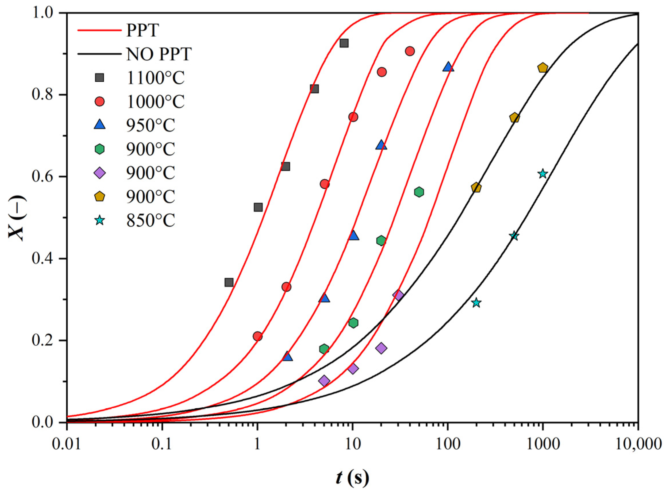
The experimental data were fitted with Avrami S-curves so that the sum of the squares of the deviations of the measured values from these curves was minimal. In the case of two-degree curves, two S-curves were used separately for the two degrees of the curves. Data occurring in the region of a constant proportion of the softened structure were not counted (see
Figure 2).
In this way, we first obtained the values of the coefficient
n in the Avrami equation (see
Table 2). First, we needed to check whether the coefficient
n is a function of temperature, as some authors state, or whether it is affected by other influences.
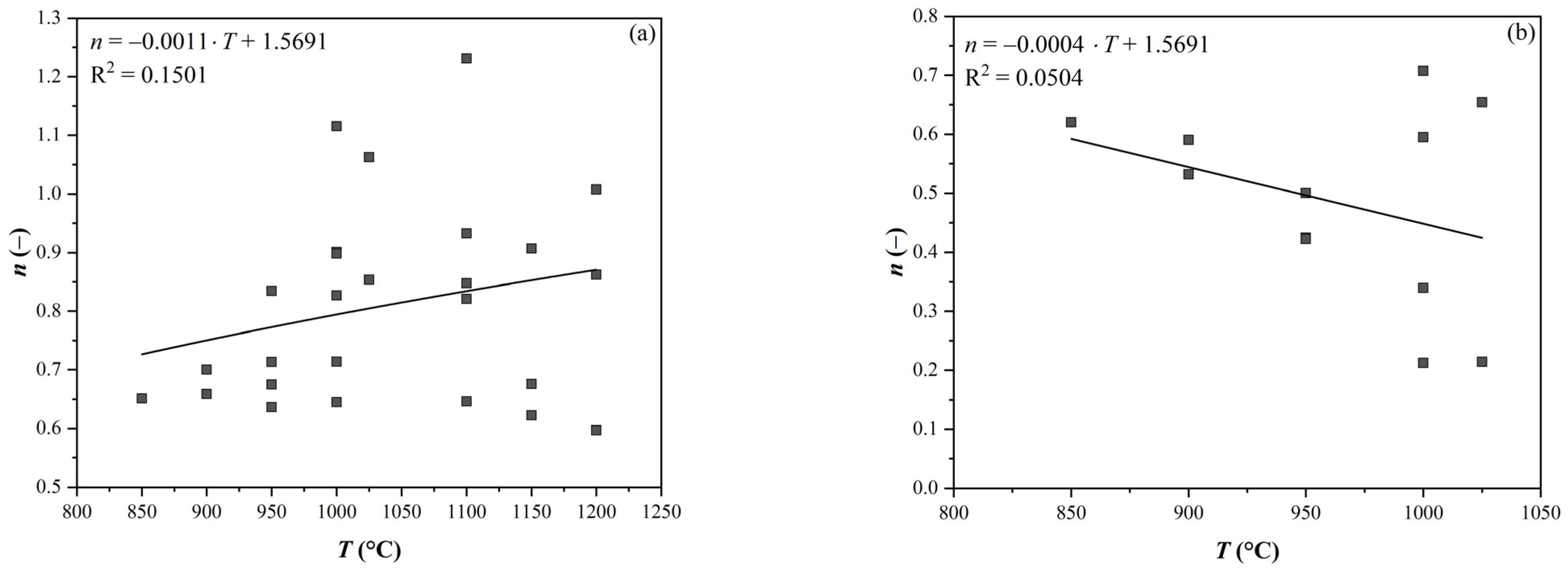
The negligible effect of temperature on the coefficient
n is illustrated in
Figure 3. The effect of the Nb content and strain size was similar.
Finally, the value of
n was determined as the average for the curves without SIP (
n = 0.823) and with SIP (
n = 0.484). These values were used to correct the S-curves in the plots similar to
Figure 2 (separately for each of the 3 steels and for the 2 strain values of 0.2 and 0.35). By varying the value of the
n coefficient in each curve, the curves were shifted towards the optimum based on the least squares method. Therefore, the position of the curves was changed again so that the minimum sum of the squares of the deviations of the measured points from the S-curves was again achieved. From the curves thus generated, a
t0.5 value was determined for each curve separately (see
Table 3).
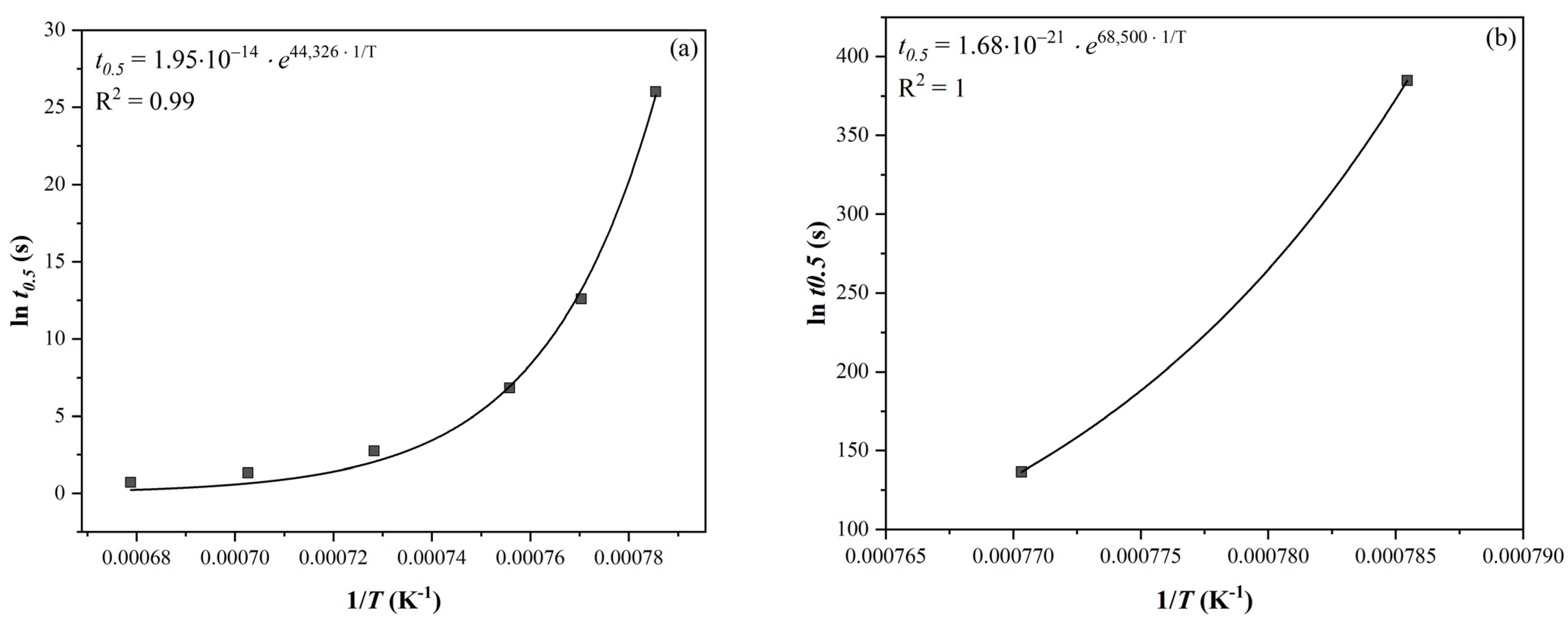
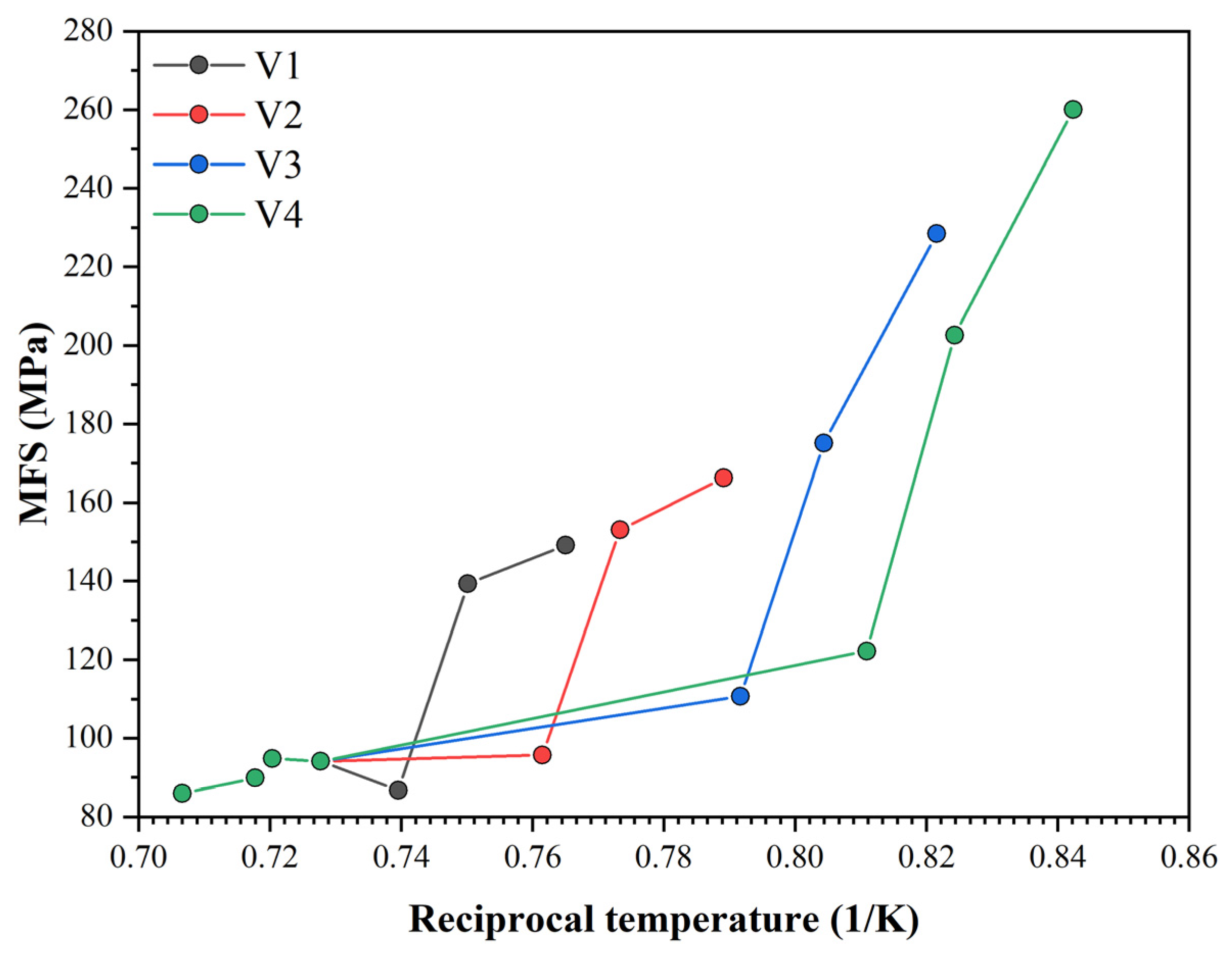
The data from
Table 3 were plotted against the reciprocal thermodynamic temperature (see
Figure 4). The activation energy values (exponent multiplied by the molar gas constant; see
Table 4) and the value of the
K constant were determined using exponential regression.
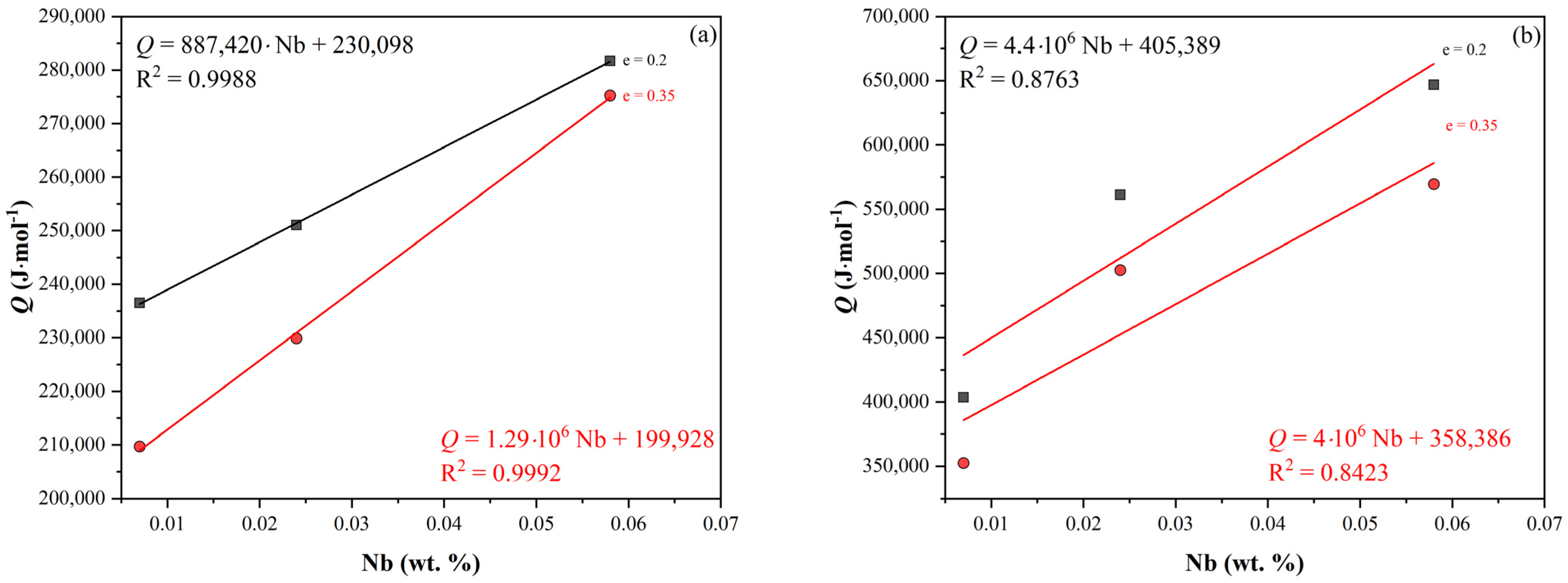
The graph in
Figure 5 shows the activation energy of the studied steels as a function of the Nb content and strain value in both the non-SIP and SIP conditions. In both cases, there seemed to be a statistically significant dependence, so the activation energy values were determined by multilinear regression as a function of the Nb content and strain in the form:
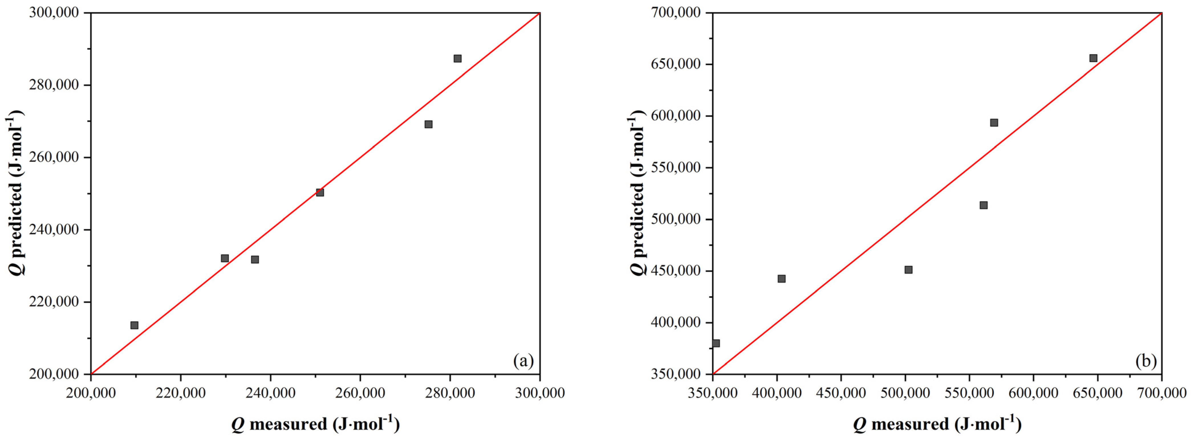
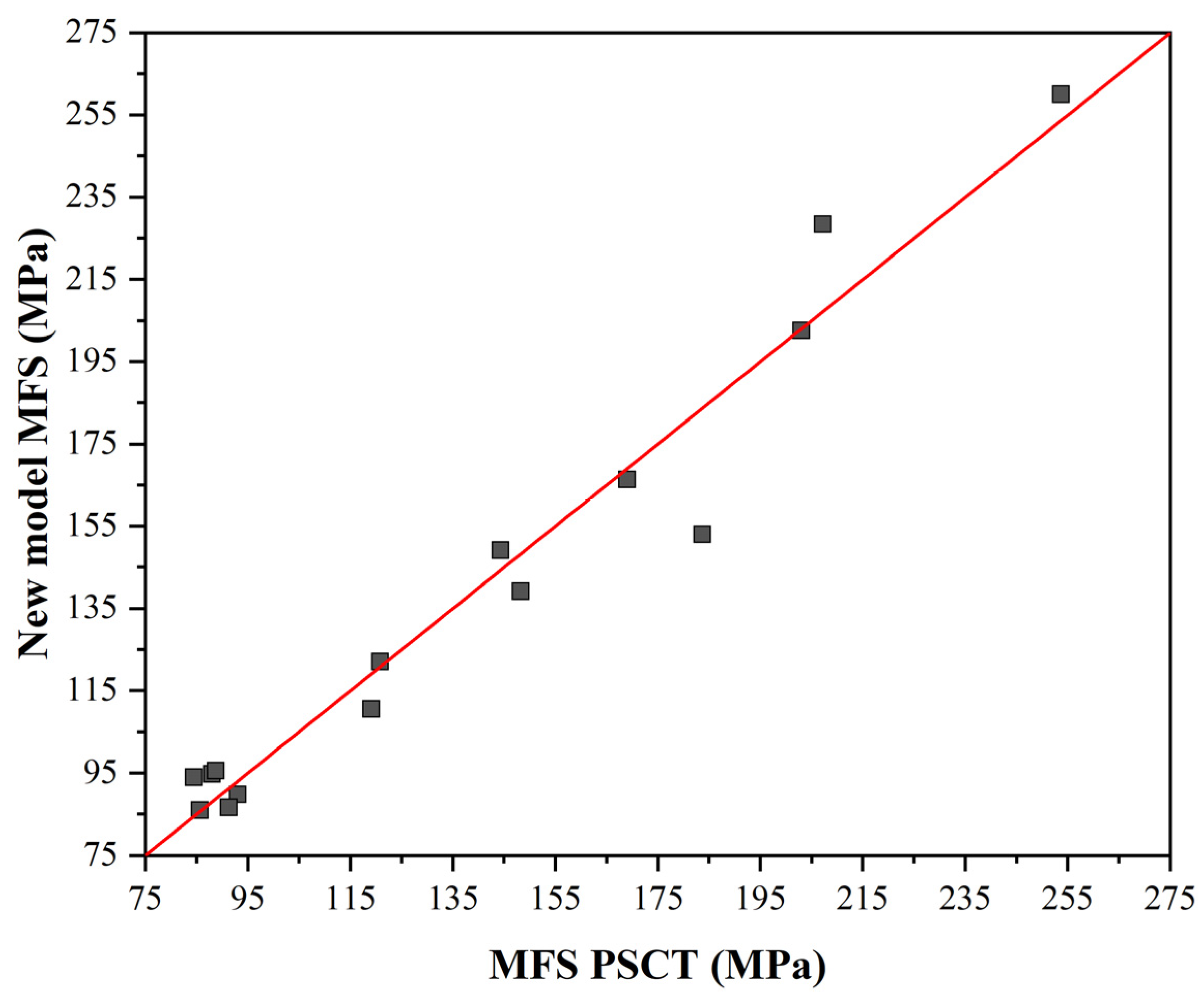
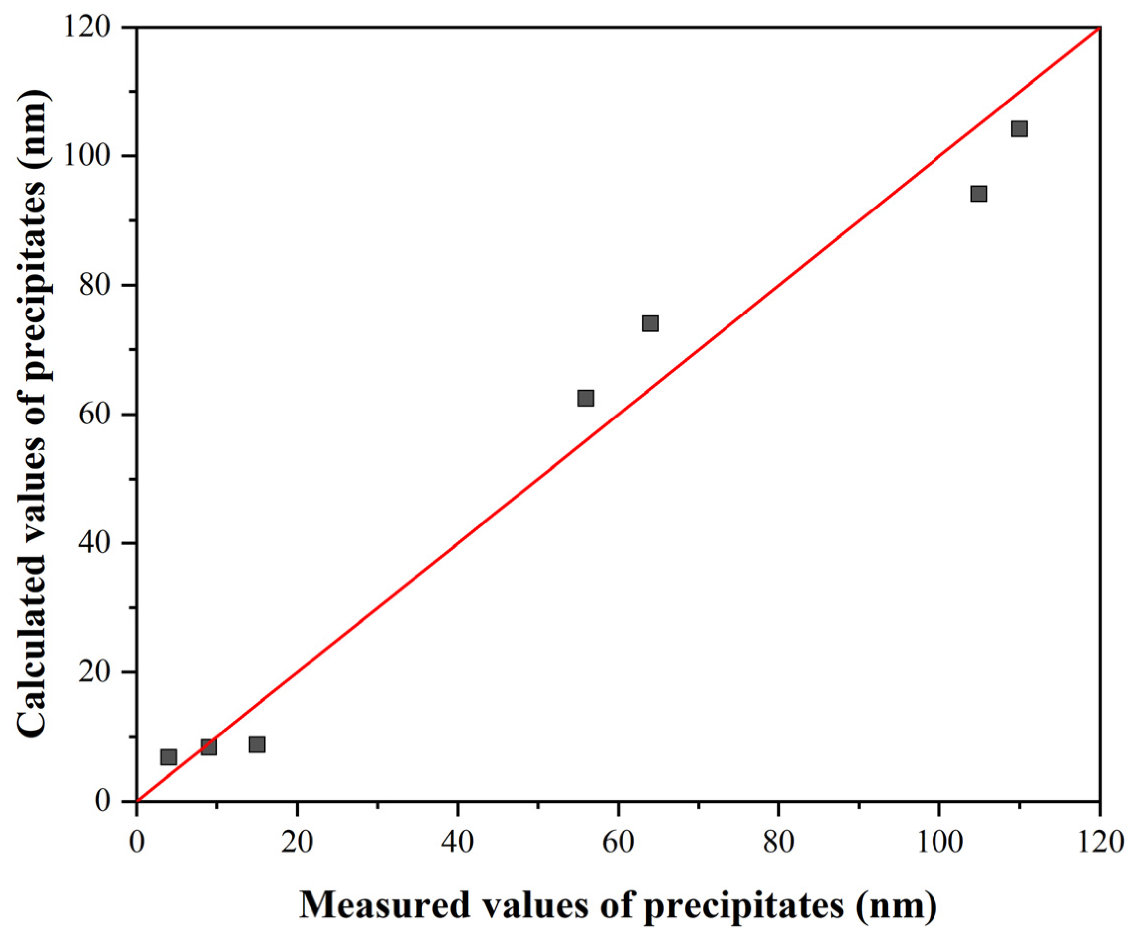
A comparison of the measured and calculated values according to Equations (1) and (2) is made in
Figure 6.
The equations obtained to describe t0.5 had the following form:
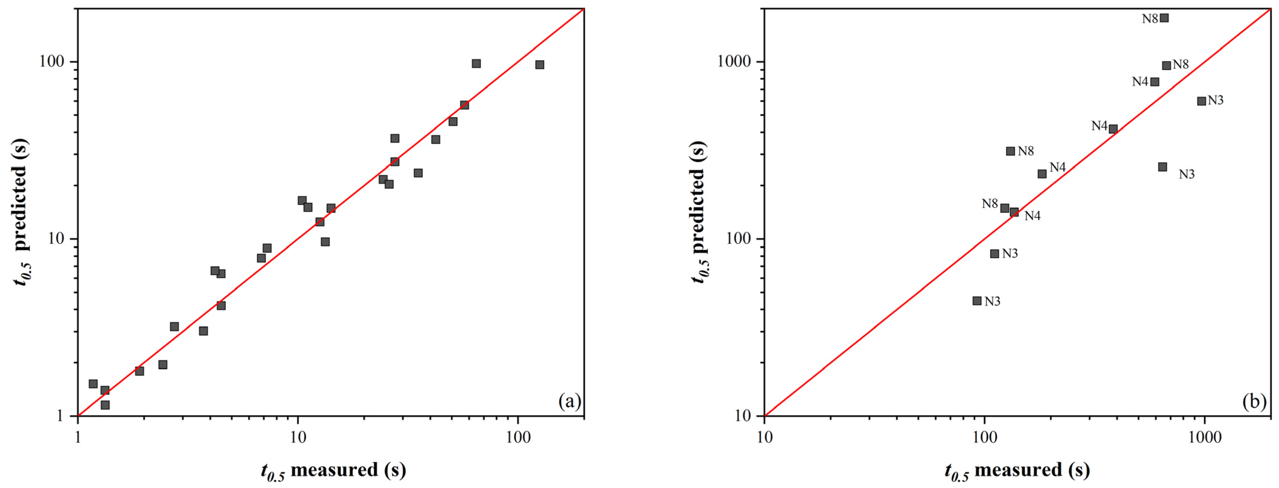
The comparison of the measured values according to Equations (3) and (4) is shown in the plot in
Figure 7. The conformity between the measured and calculated values for
t0.5 without SIP is good, but in the case of
t0.5 with SIP, the scatter of the data around the mean line is visibly worse. The arrangement of the data into layers by steel number can be seen here (data labels in the plot in
Figure 7b). All
t0.5 values are below the mean line for N3 steel, while the opposite is true for N8 steel. Apart from the Nb content, the steels used differ mainly in the Mn and Si content ratio, significantly affecting Nb precipitation. This effect is more pronounced in steels with a higher Nb content because the solubility of Nb in steel decreases with an increasing Mn/Si ratio. Therefore, Equation (4) was modified to the following form:
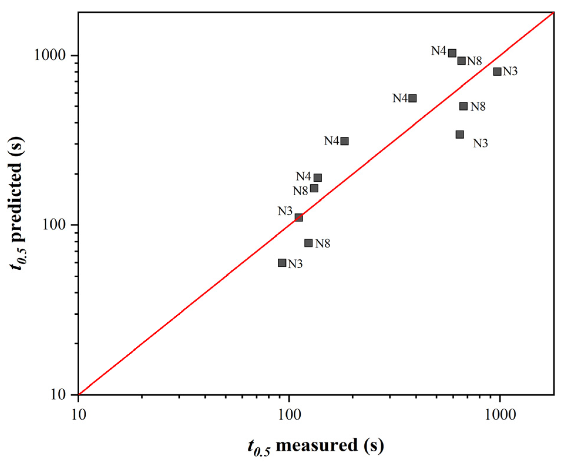
Using this correction factor, the scatter of values around the mean line was minimized (
Figure 8). If the data were further refined, more measured softening curves’ data would be required for the variant with SIP.
Since in the experiment from which our data were taken, the grain size ranged from 140 to 210 μm, it was necessary to add a term to the equations to describe
t0.5 to account for the change in grain size during actual rolling. The effect of grain size
D was included in previous equations in the following form:
where
D′ is the average value of the grain size used in the experiment (180 μm).
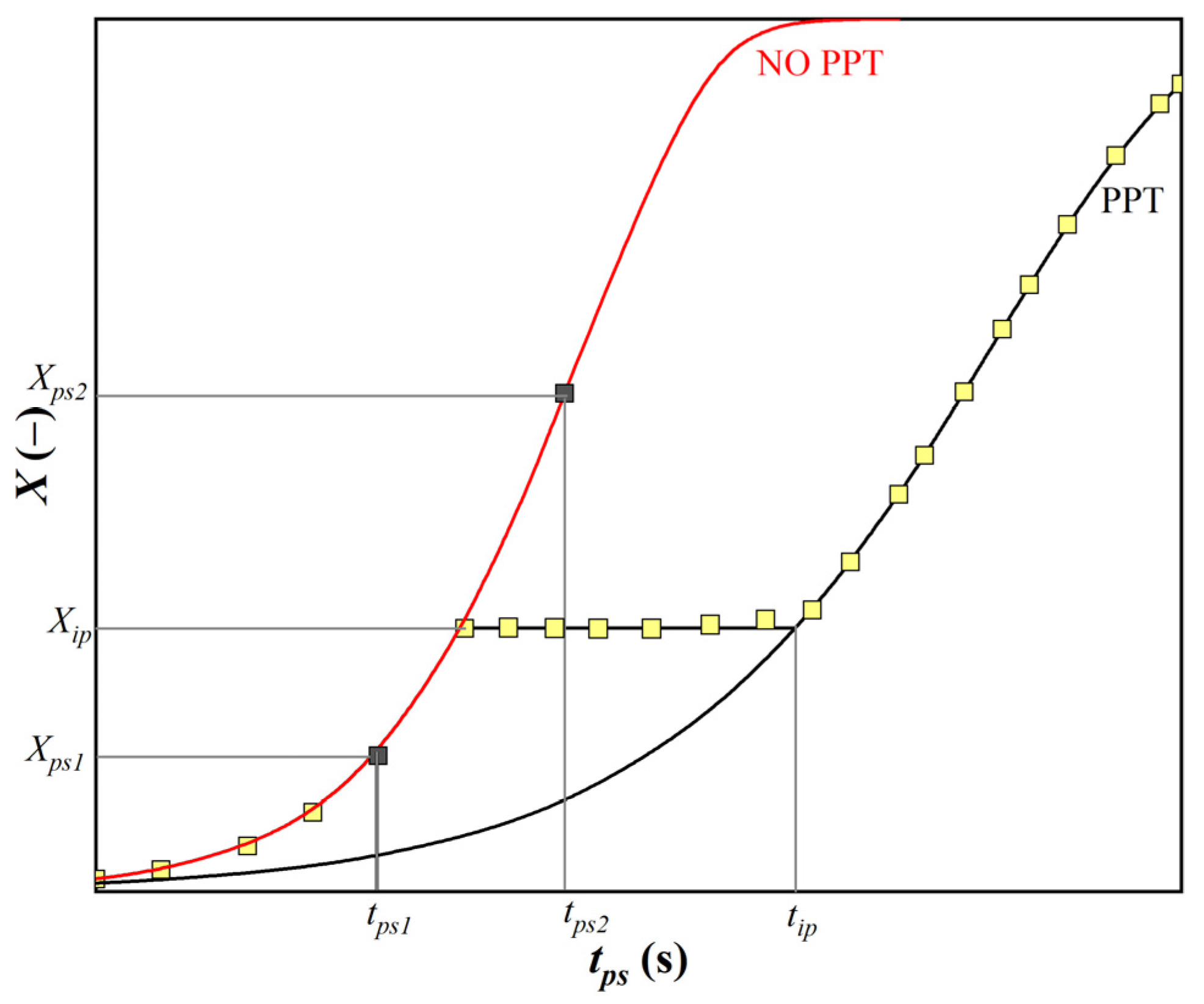
To use the equations obtained to describe
t0.5 in the microstructure evolution model, it is necessary to solve the determination of
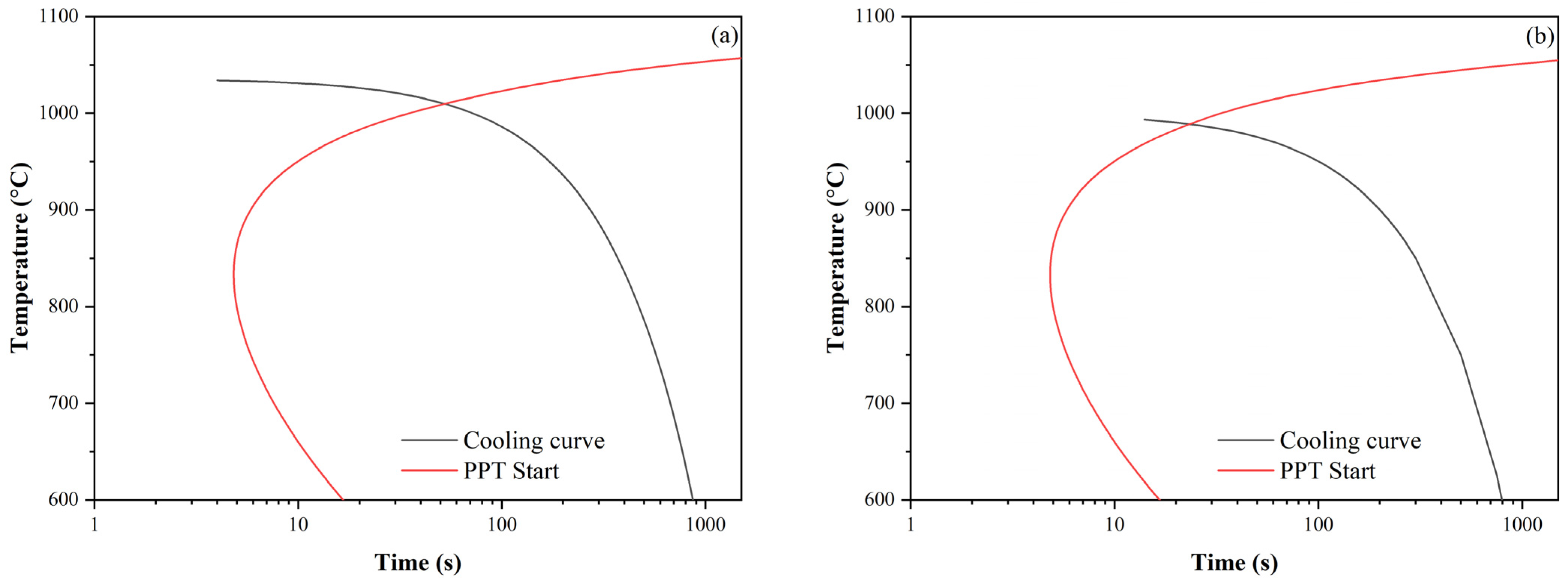
t0.5 in the pass in which the SIP occurs. In this pass, it is assumed that
tip >
tps. The following two situations can occur (see
Figure 9). The fraction of the softened structure at time
tip for a curve with SIP is
- −
greater than the proportion of the softened structure at time
tps for the curve without SIP (
tps1 and
Xtps1 in
Figure 9);
- −
less than the proportion of the softened structure at time
tps for the curve without SIP (
tps2 and
Xtps2 in
Figure 9).
In the first case, the model will calculate the X values from the SIP curve and vice versa in the second case.
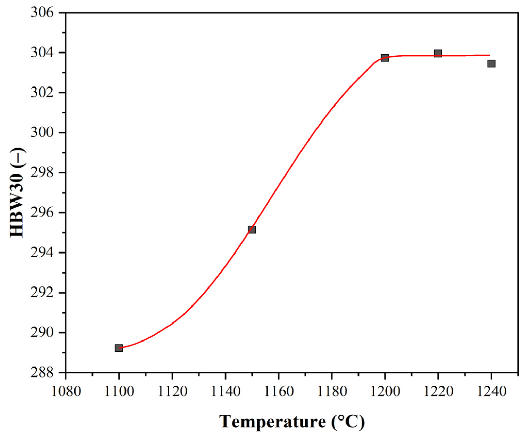
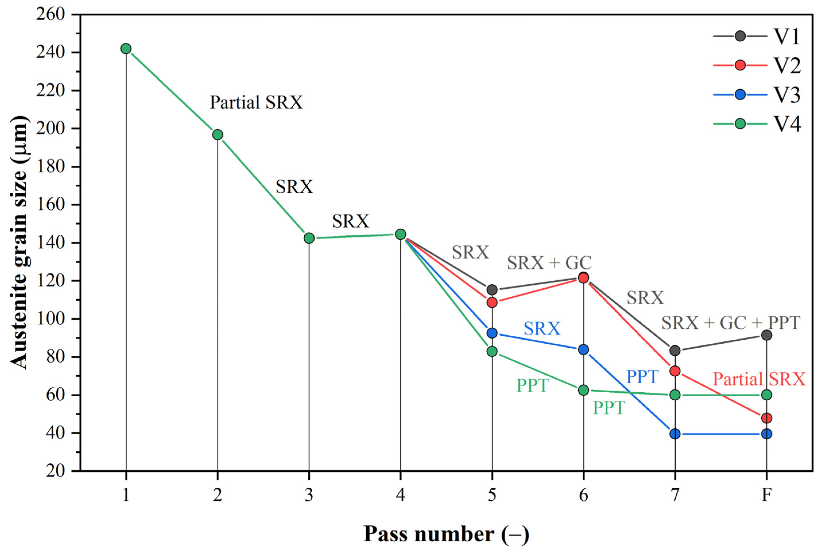
The last point of the model modification is the modification of the parameters of the Hodgson equation [
37] for the grain size calculation after static recrystallization. The data obtained from the PSCT (see the next section) showed that our HSLA steel has a significantly coarser grain. The modified equation has the following form:

 ,
, 


 represents an individual pass).


