
Facet Connectivity-Based Estimation Algorithm for Manufacturability of Supportless Parts Fabricated via LPBF
 , , , , , and
Abstract
:1. Introduction
2. Algorithm for Supporting Effect
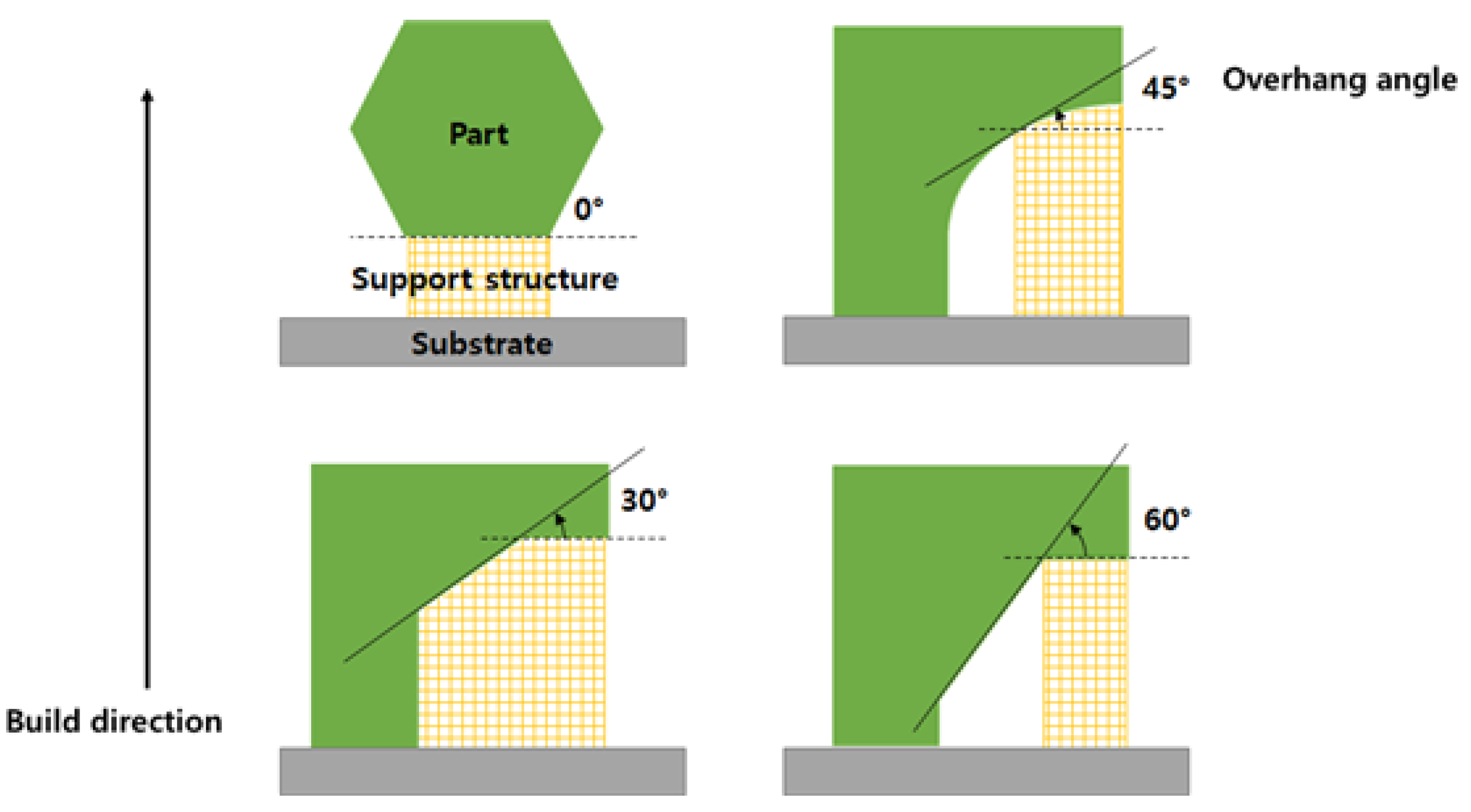
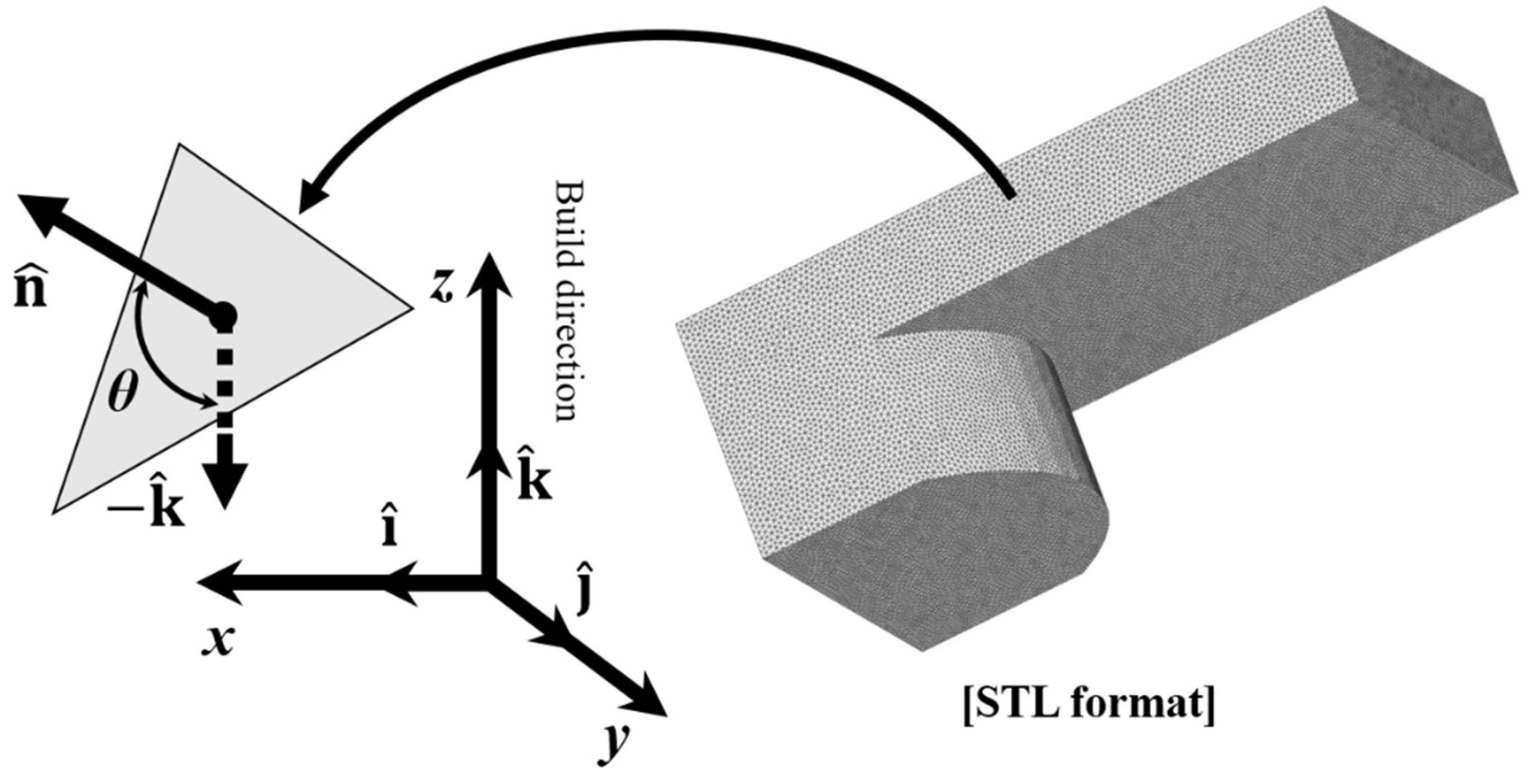
2.1. Facet Orientation Angle Estimation
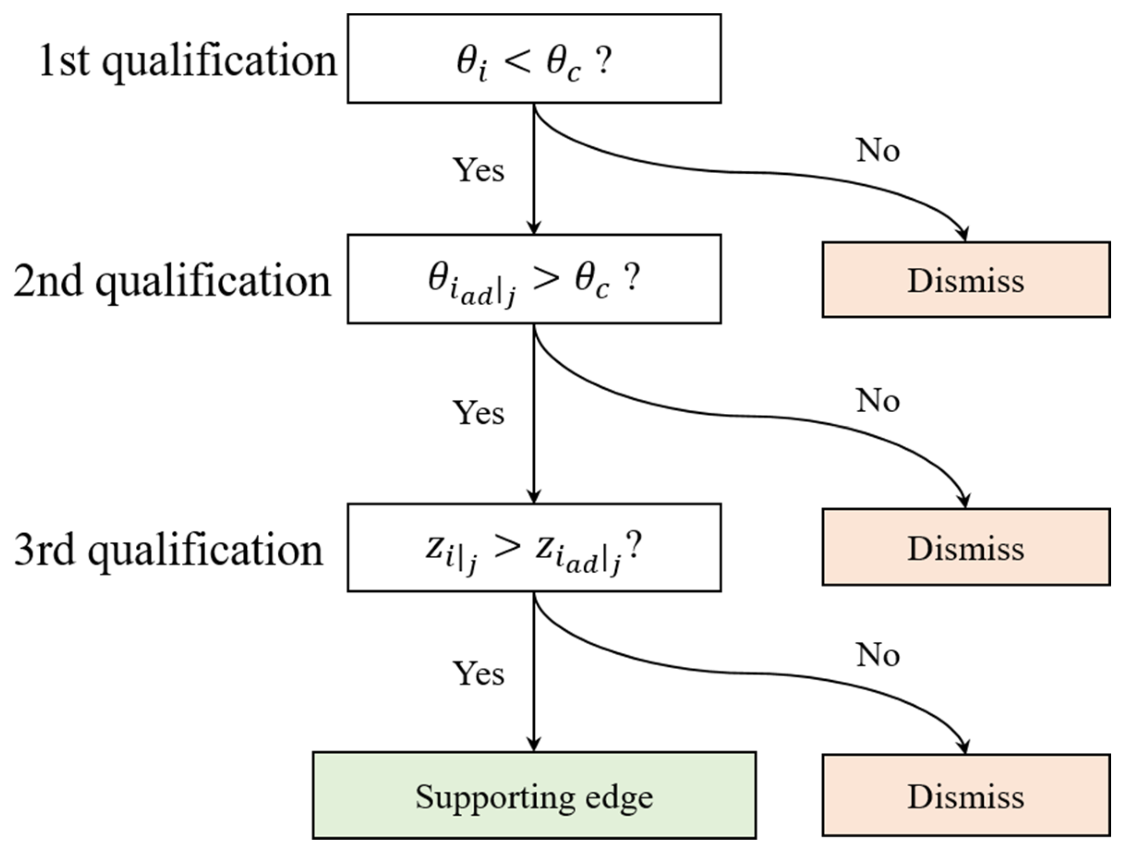
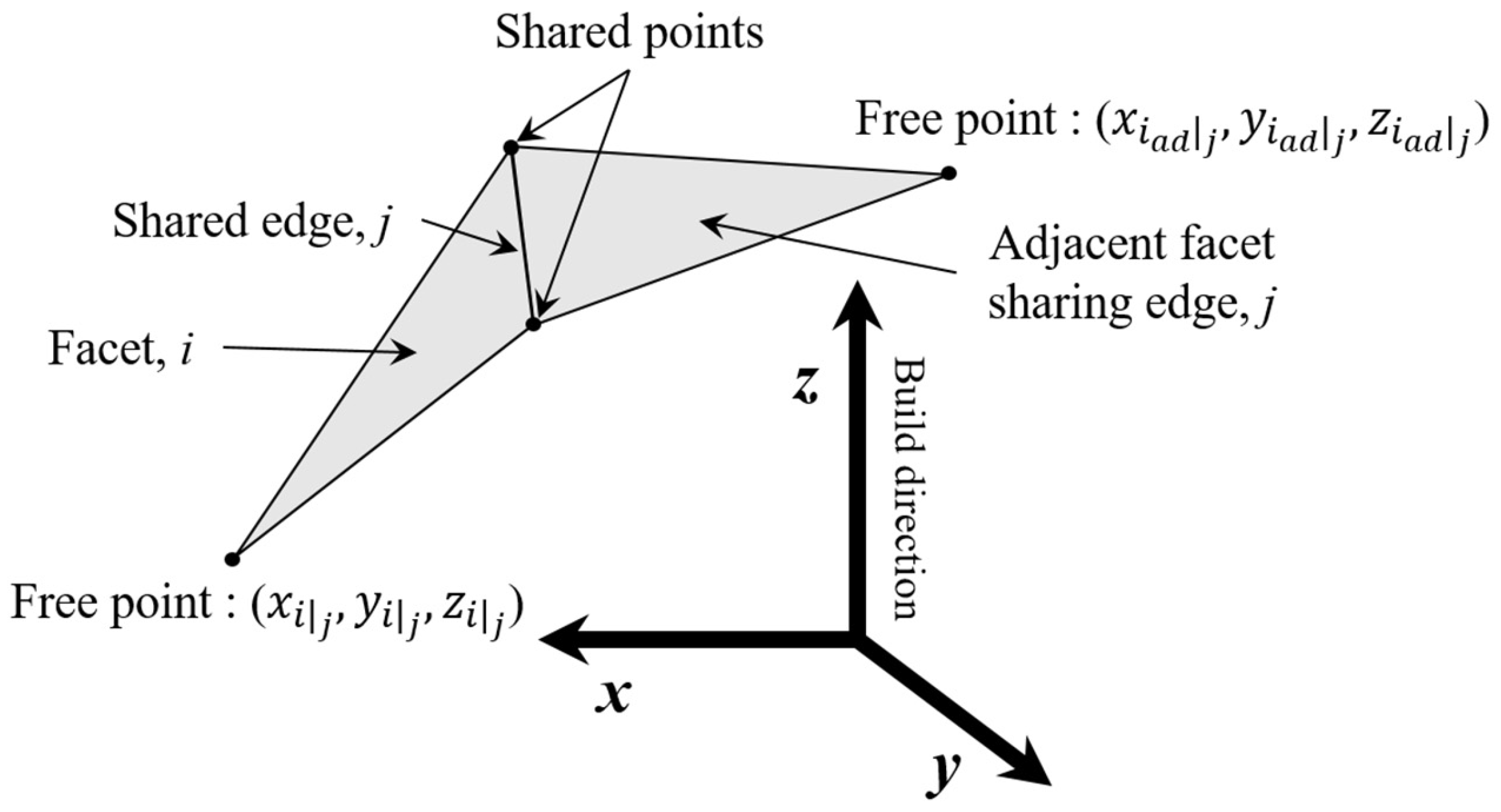
2.2. Initial Step for Assigning Initial Value on Supporting Boundary Edge
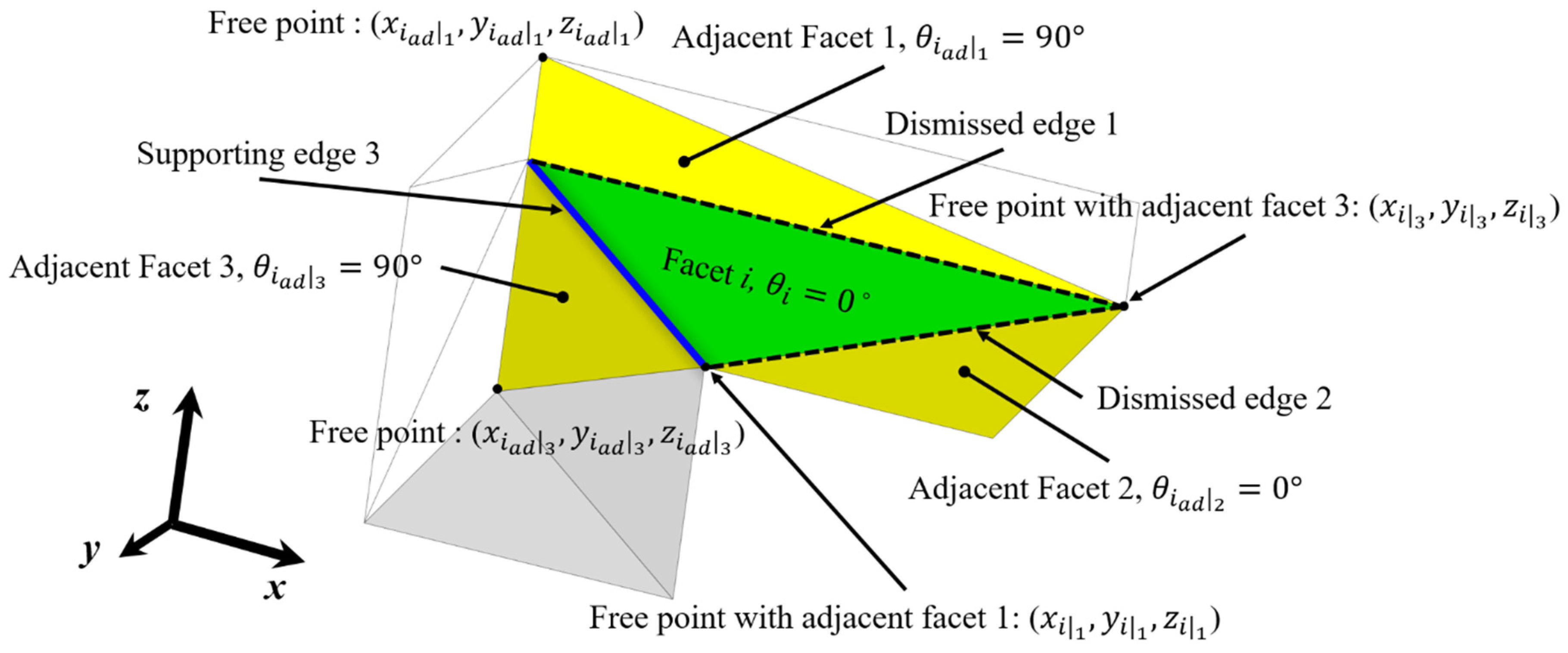
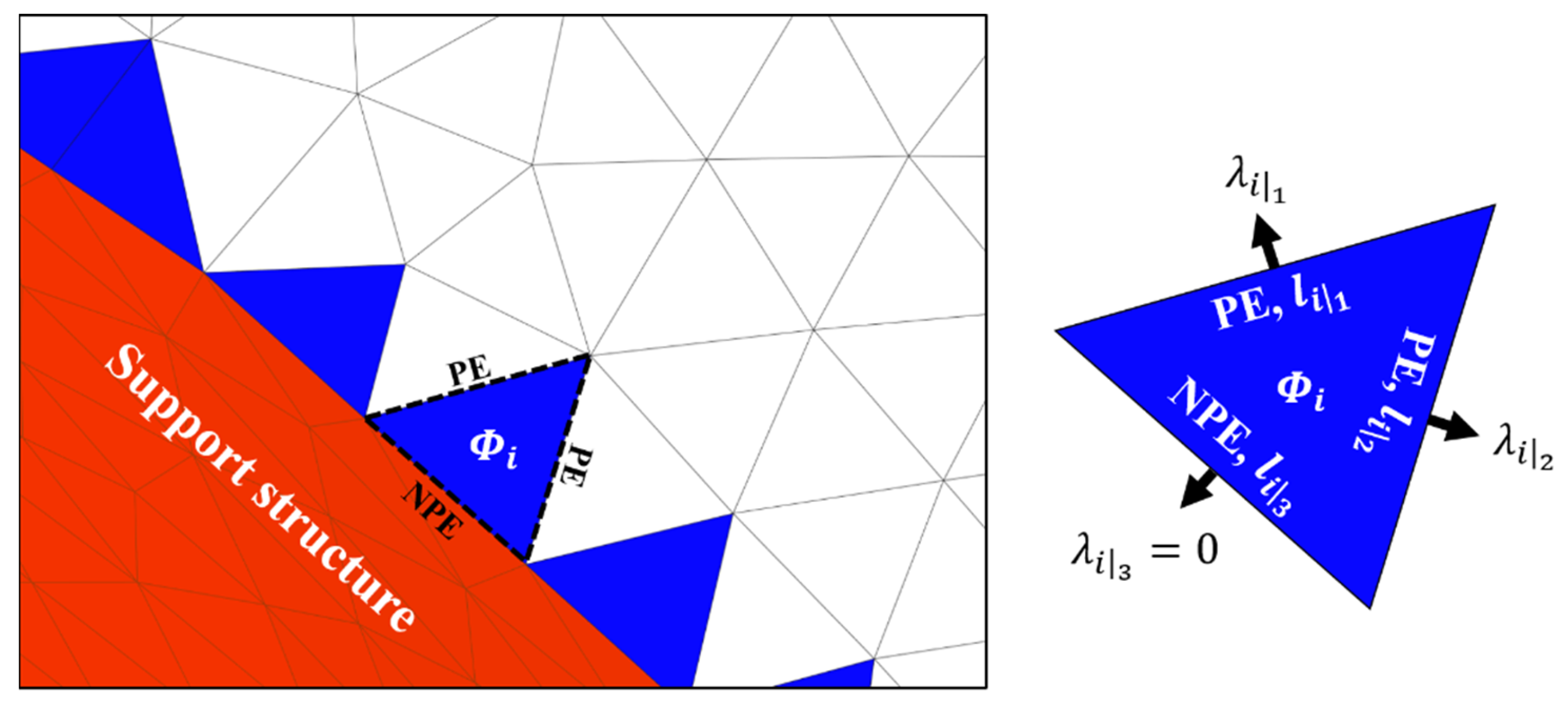
- 1.
- The shared edge between facet i and adjacent facet 1
- The orientation angle of facet i, , is smaller than the critical overhang angle, 45° (first qualification);
- The orientation angle of adjacent facet 1, , is larger than 45° (second qualification);
- The z-coordinate of a free point of facet i with adjacent facet 1, , is below the free point of adjacent facet 1, (third qualification).
- 2.
- The shared edge between facet i and adjacent facet 2
- The orientation angle of facet i, , is smaller than the critical overhang angle, 45° (first qualification);
- The orientation angle of adjacent facet 2, , is smaller than 45° (second qualification).
- 3.
- The shared edge between facet i and adjacent facet 3
- The orientation angle of facet i, , is smaller than the critical overhang angle, 45° (first qualification);
- The orientation angle of adjacent facet 3, , is larger than 45° (second qualification);
- The z-coordinate of a free point of facet i with adjacent facet 3, , is above the free point of adjacent facet 3, (third qualification).
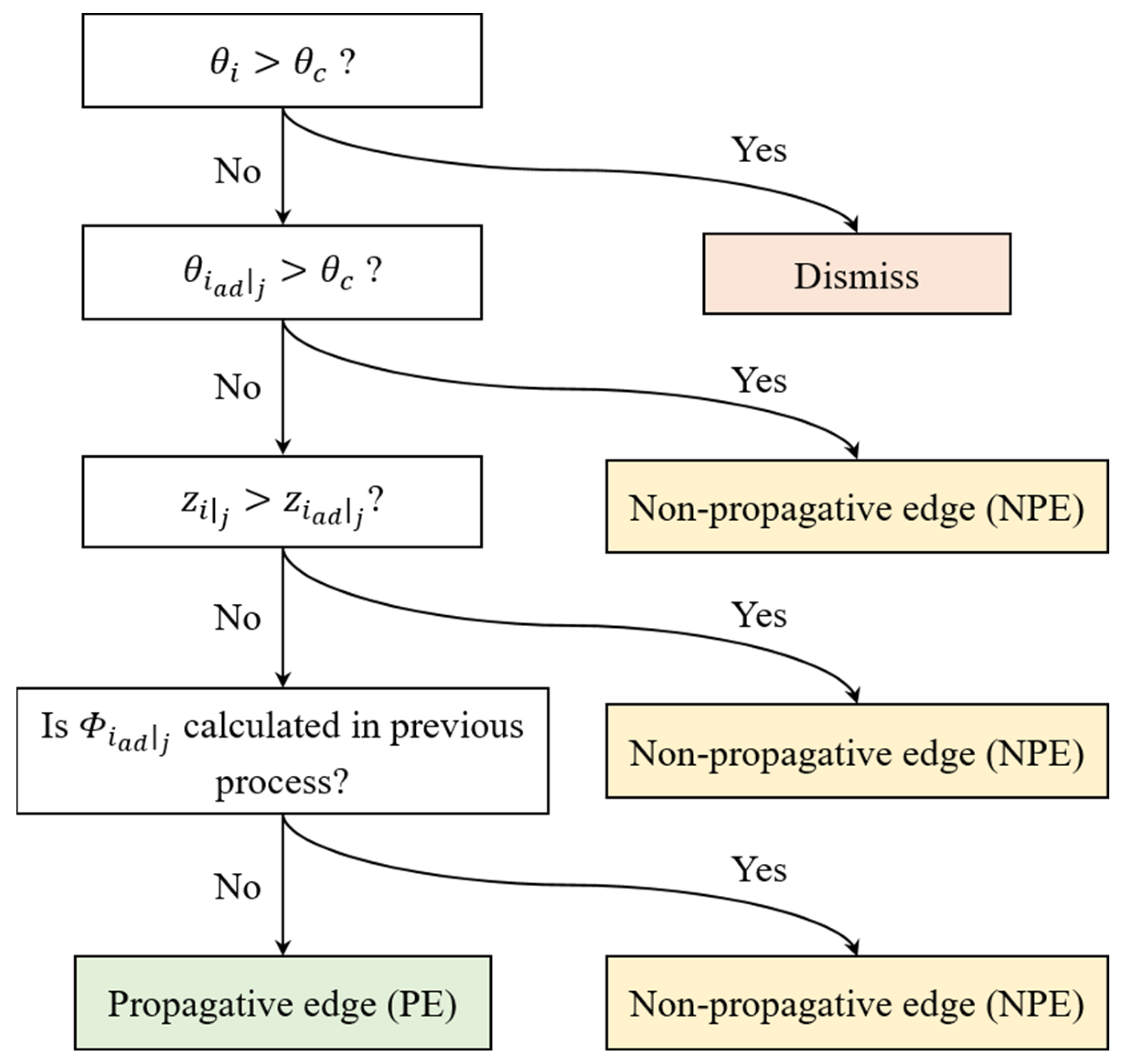
2.3. Edge Classification
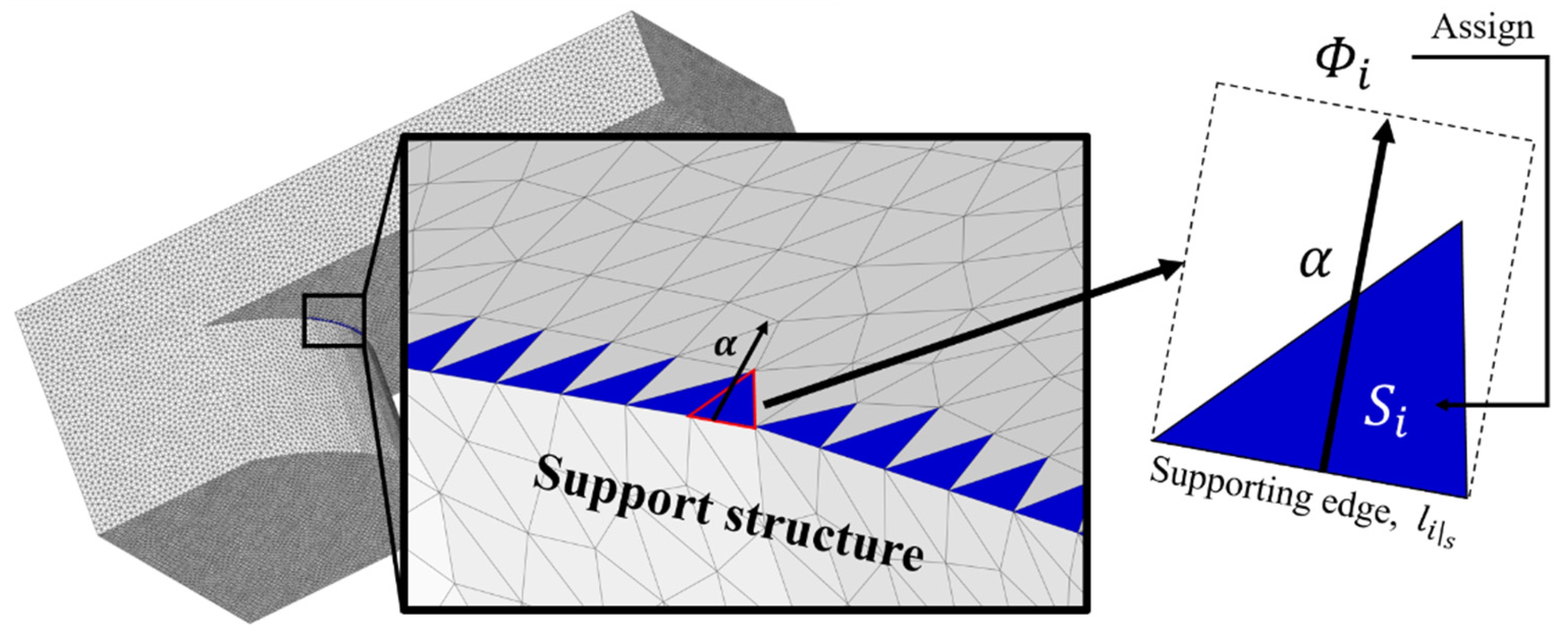
2.4. First Step for Transferring Support Effect
2.5. Second Step for Receiving Support Effect λ
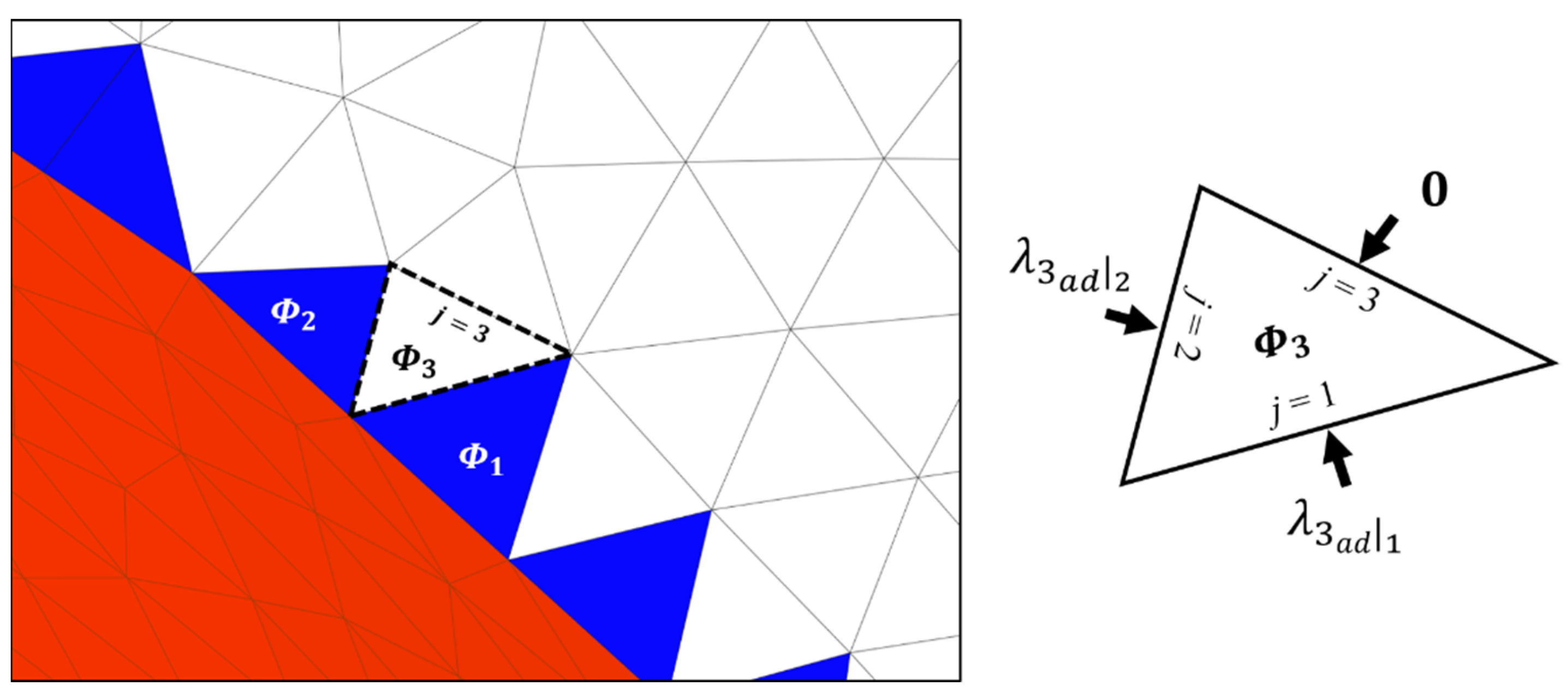
2.6. Process Demonstration
- 1.
- ,Based on Equation (3);
- 2.
- Based on Equation (4);
- 3.
- Based on Equation (5);
- 4.
- .
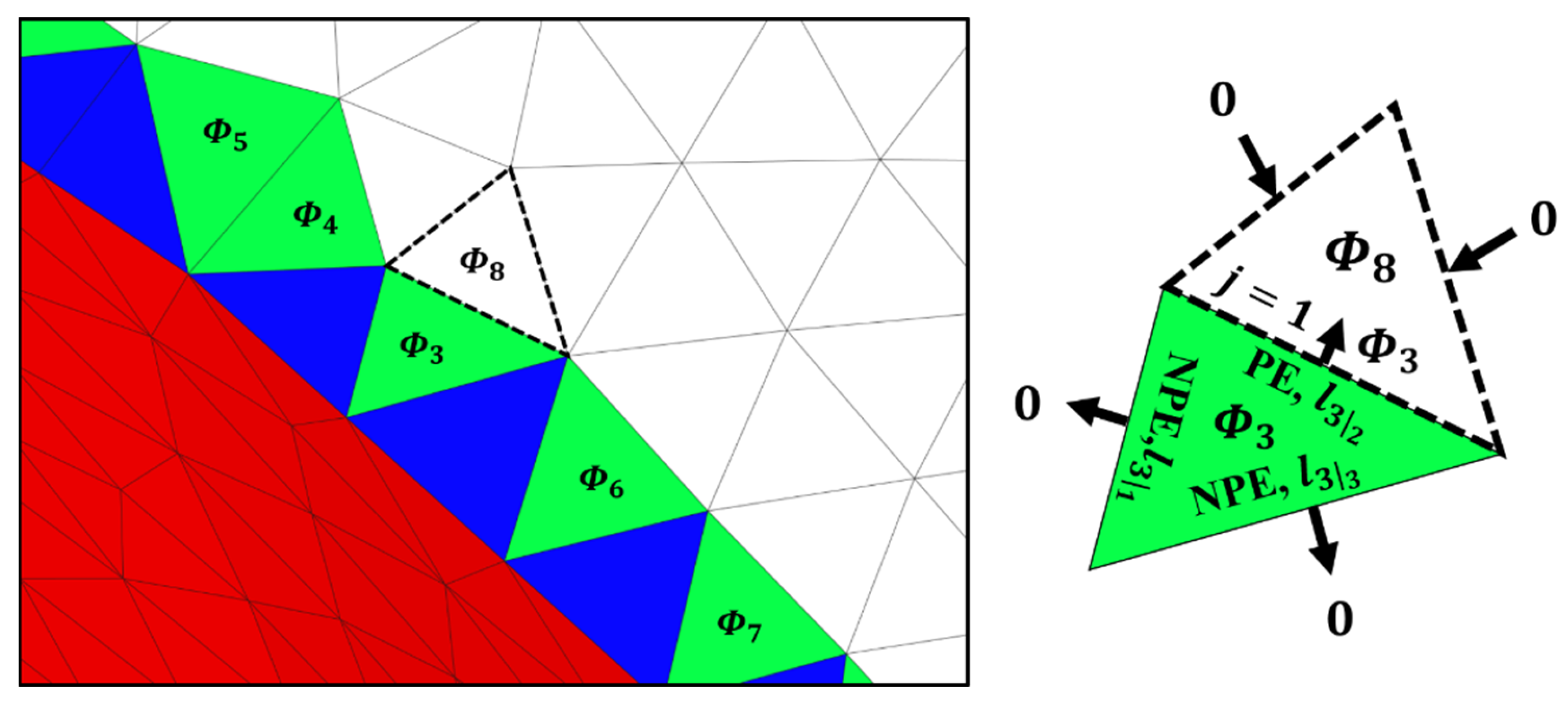
- 1.
- Based on Equations (2) and (6);
- 2.
- ;
- 3.
- .
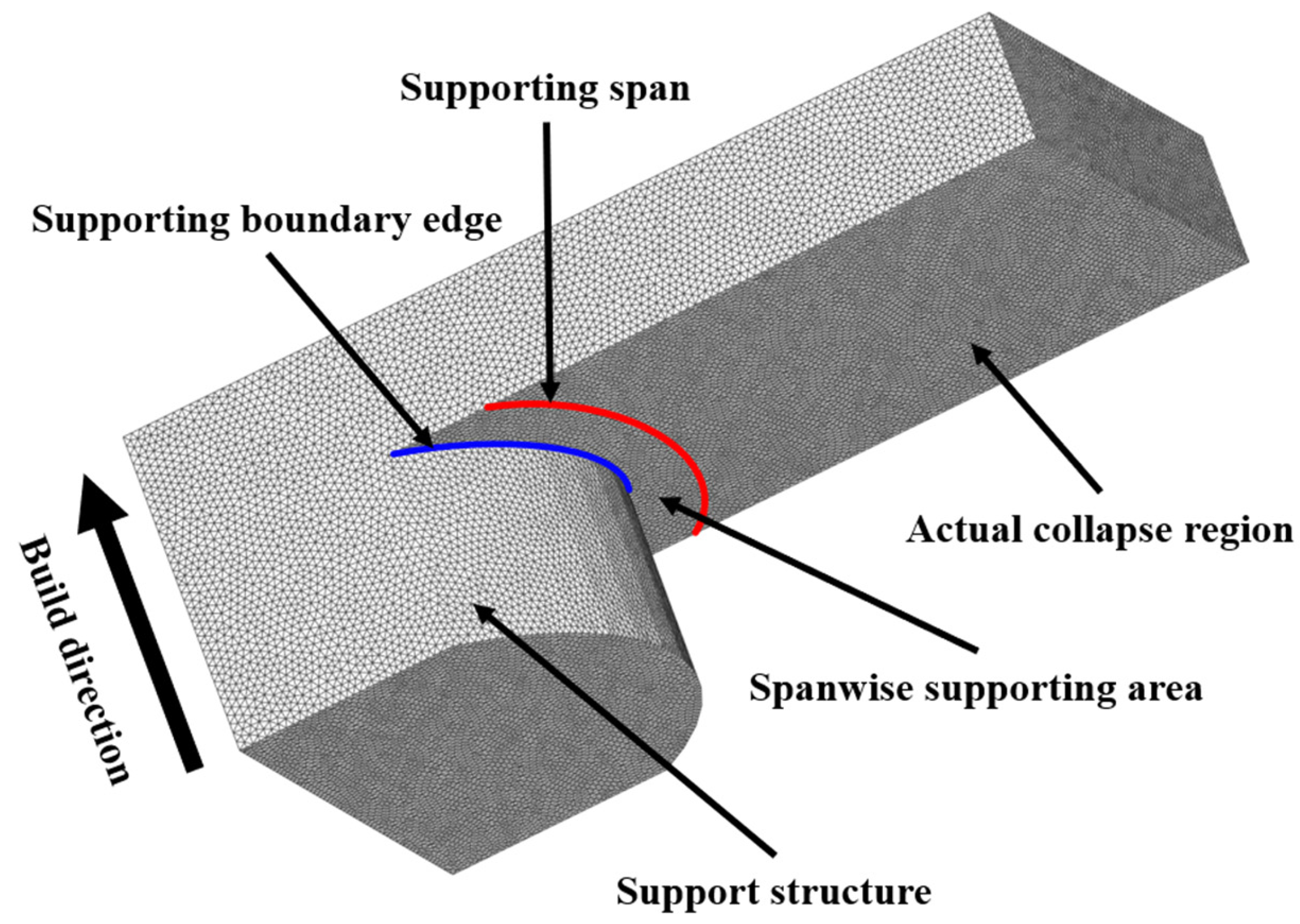
2.7. Invalidation of Overestimated Collapse Region
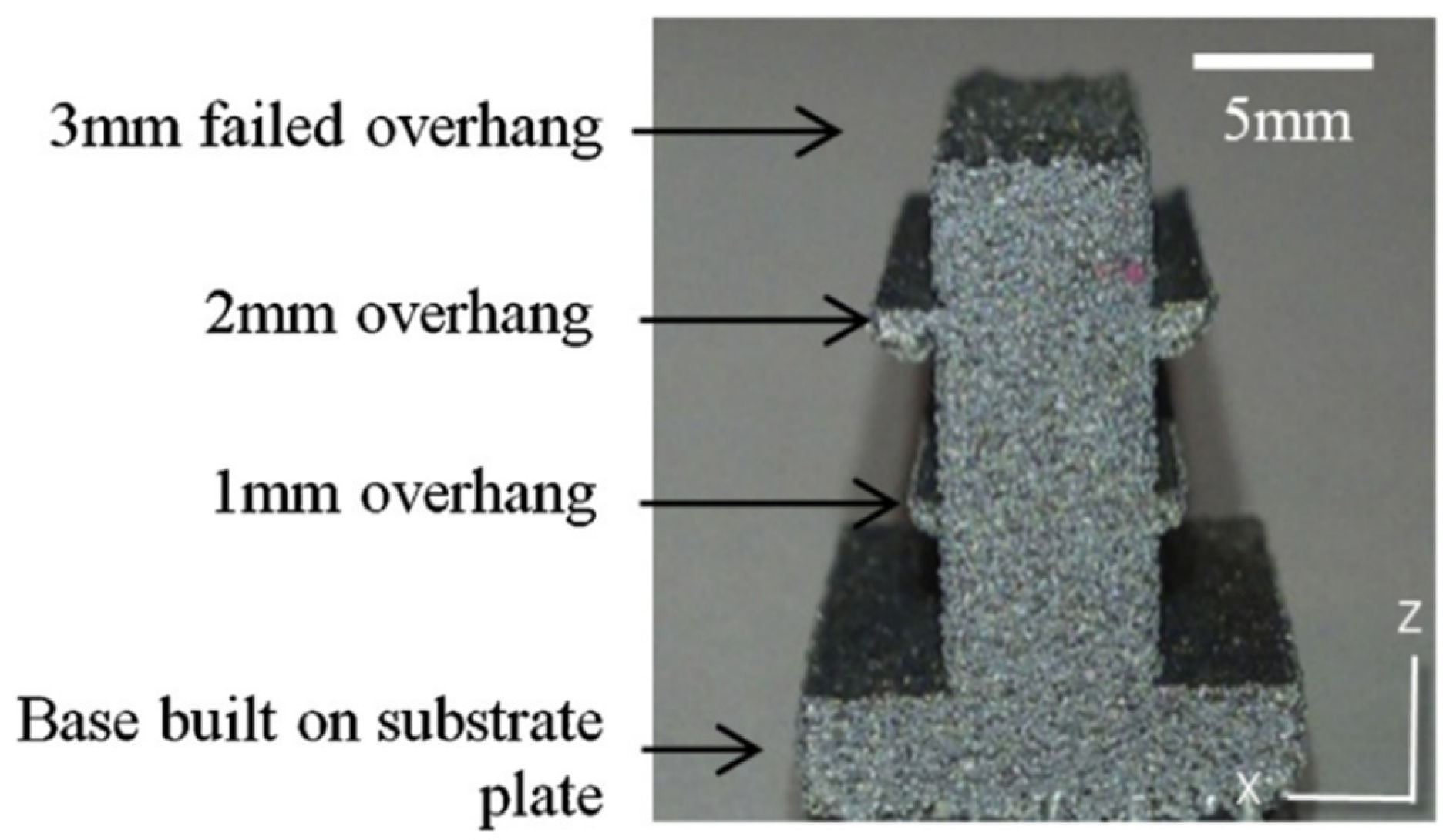
3. Experimental Validation via LPBF
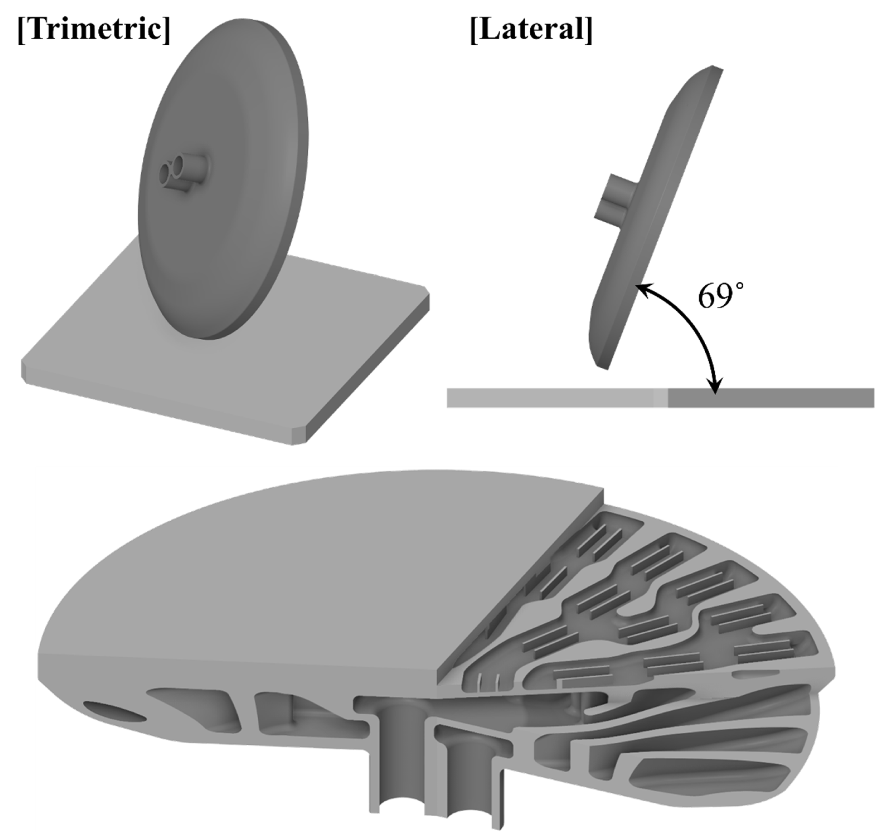
3.1. Heat Exchanger Model
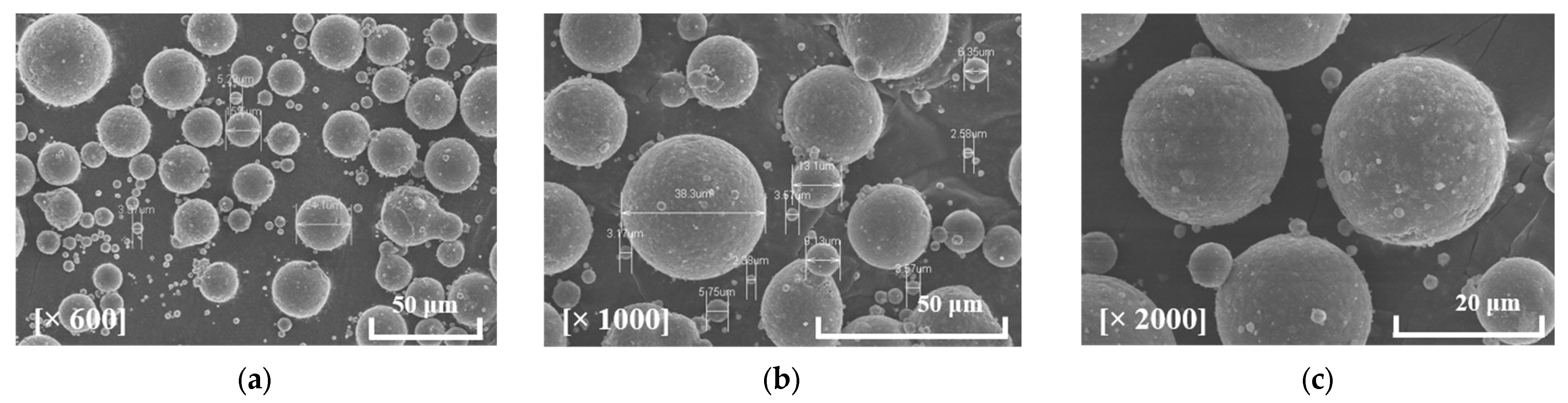
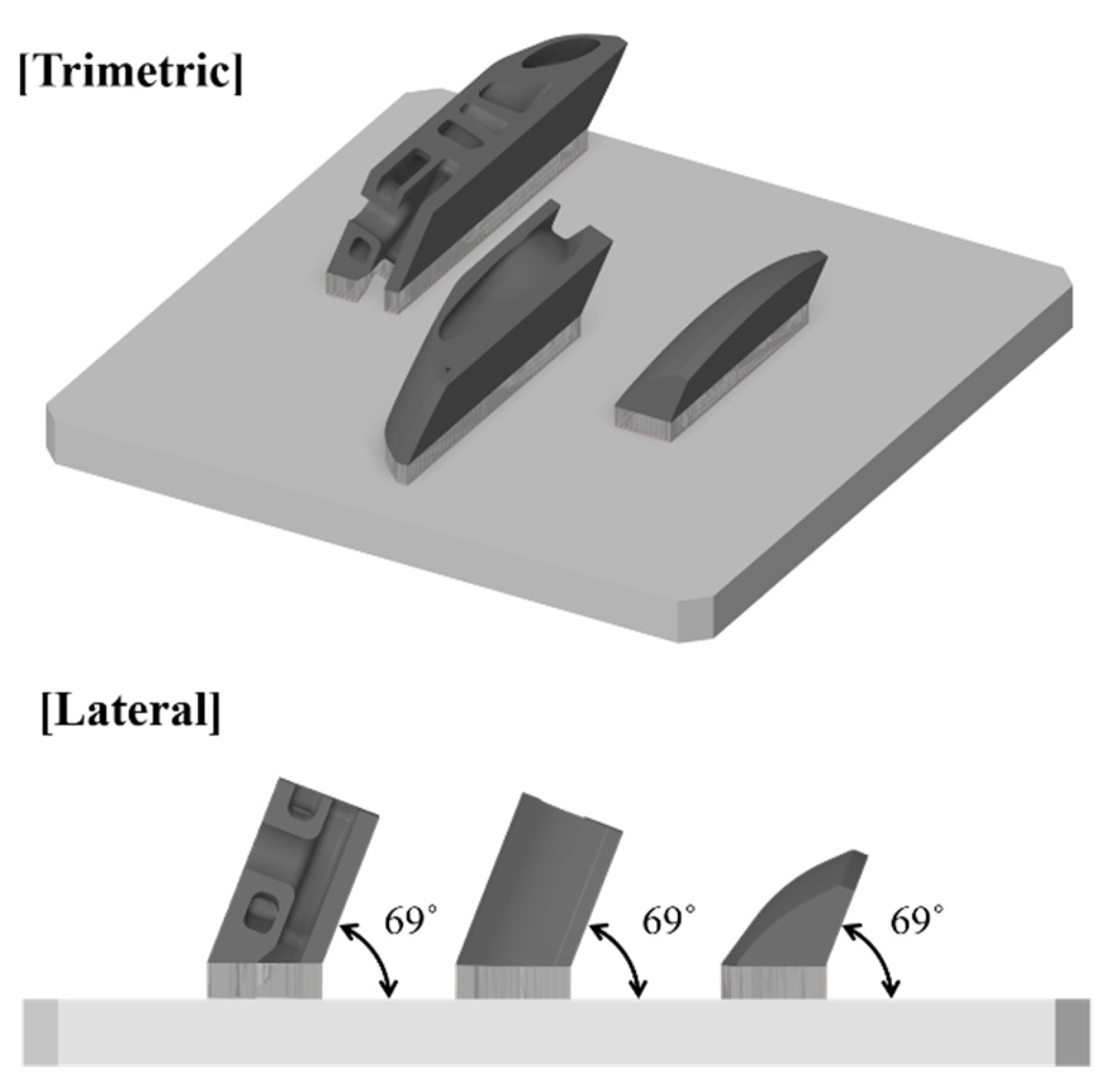
3.2. Fabrication
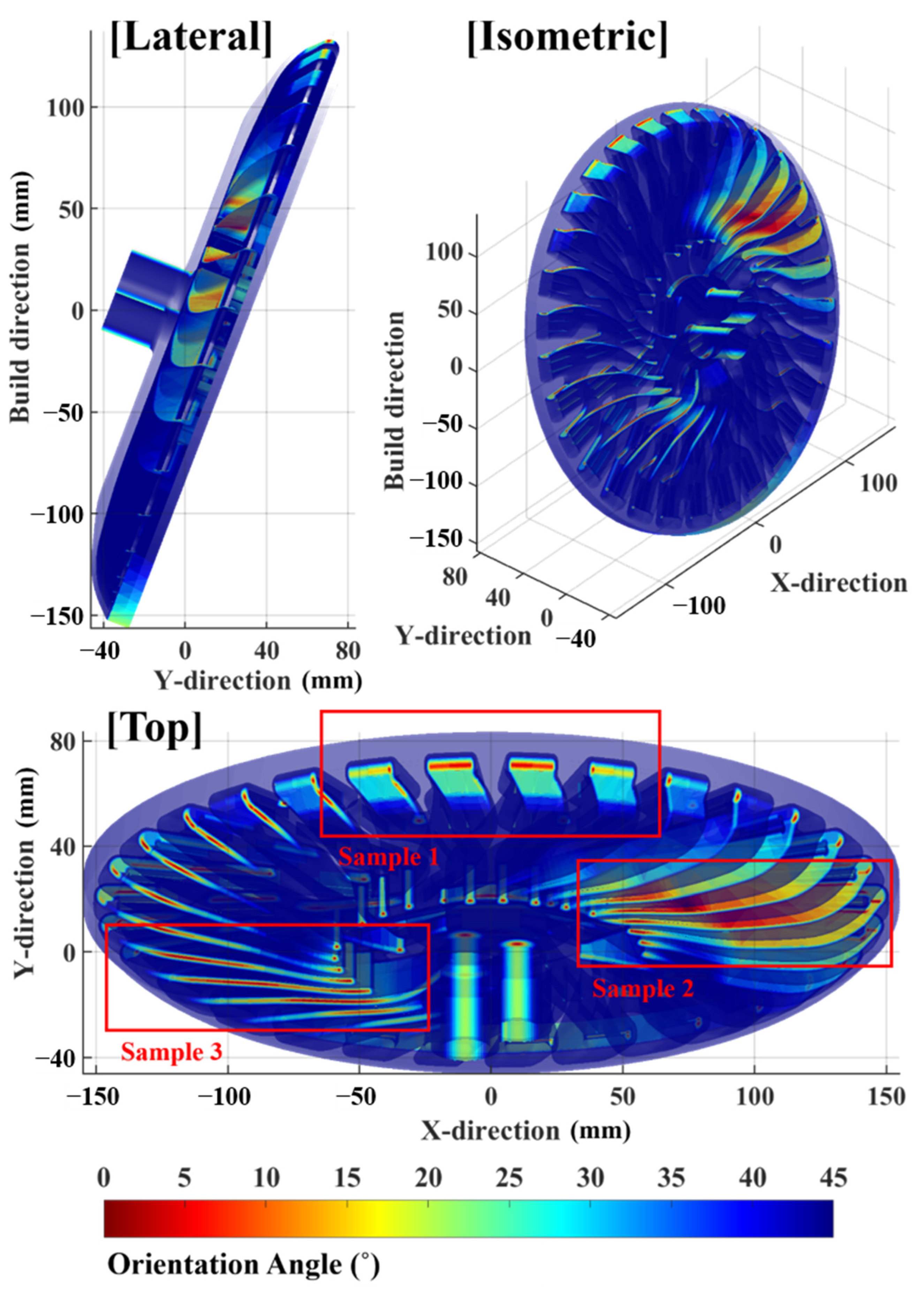
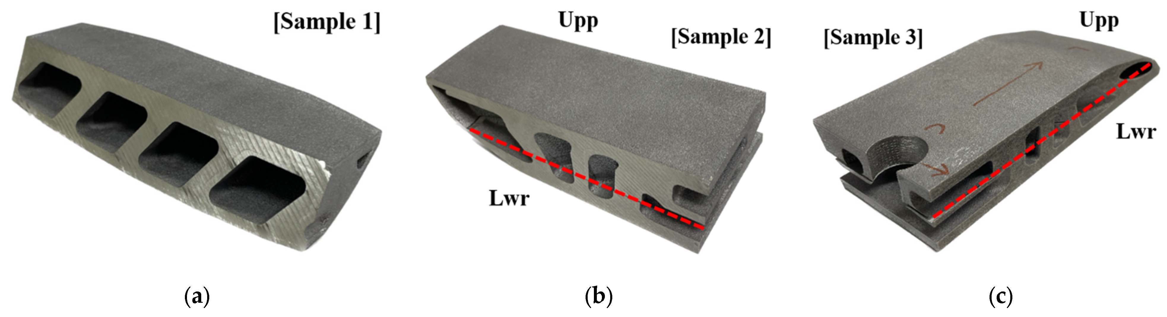
4. Results and Discussion
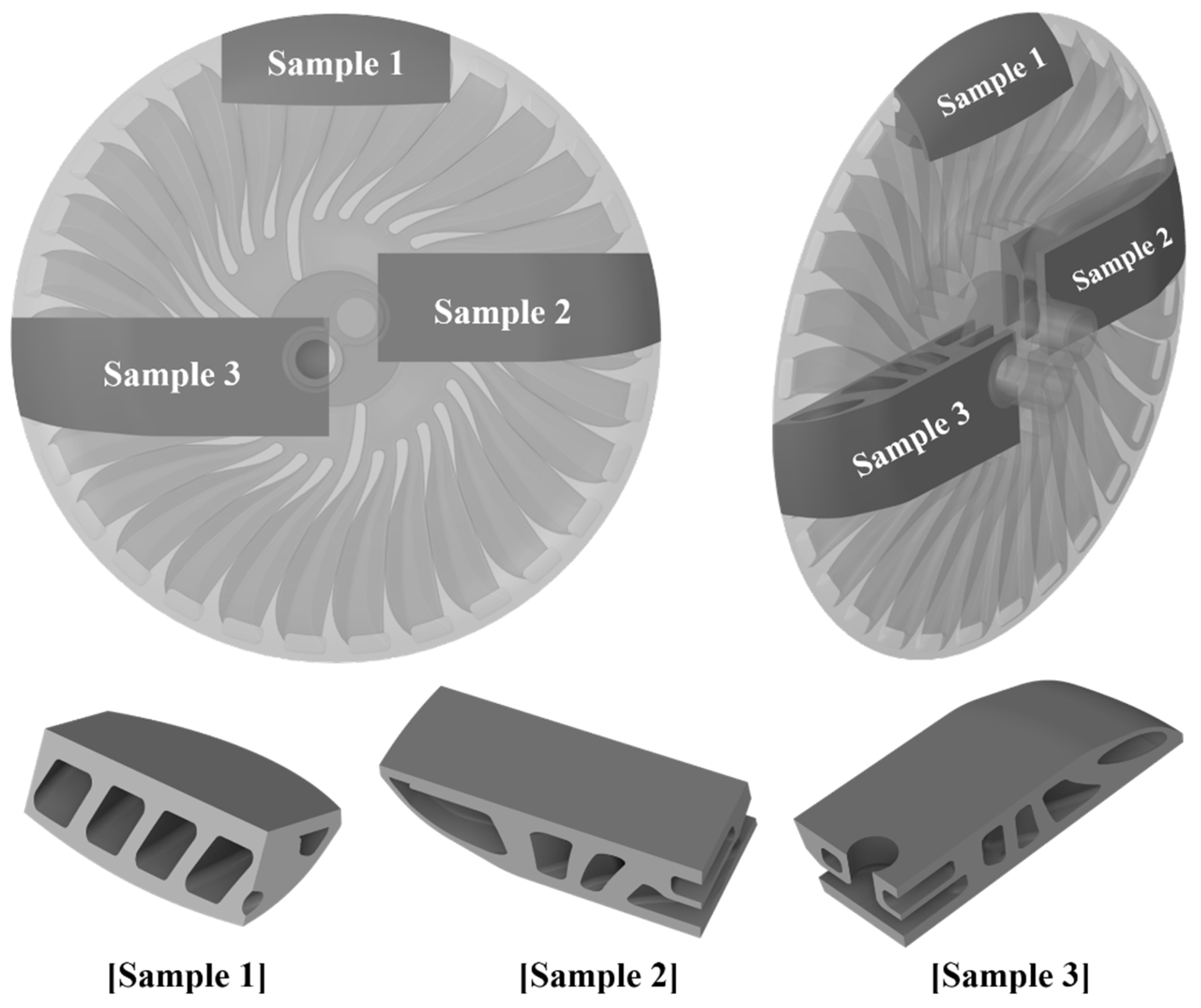
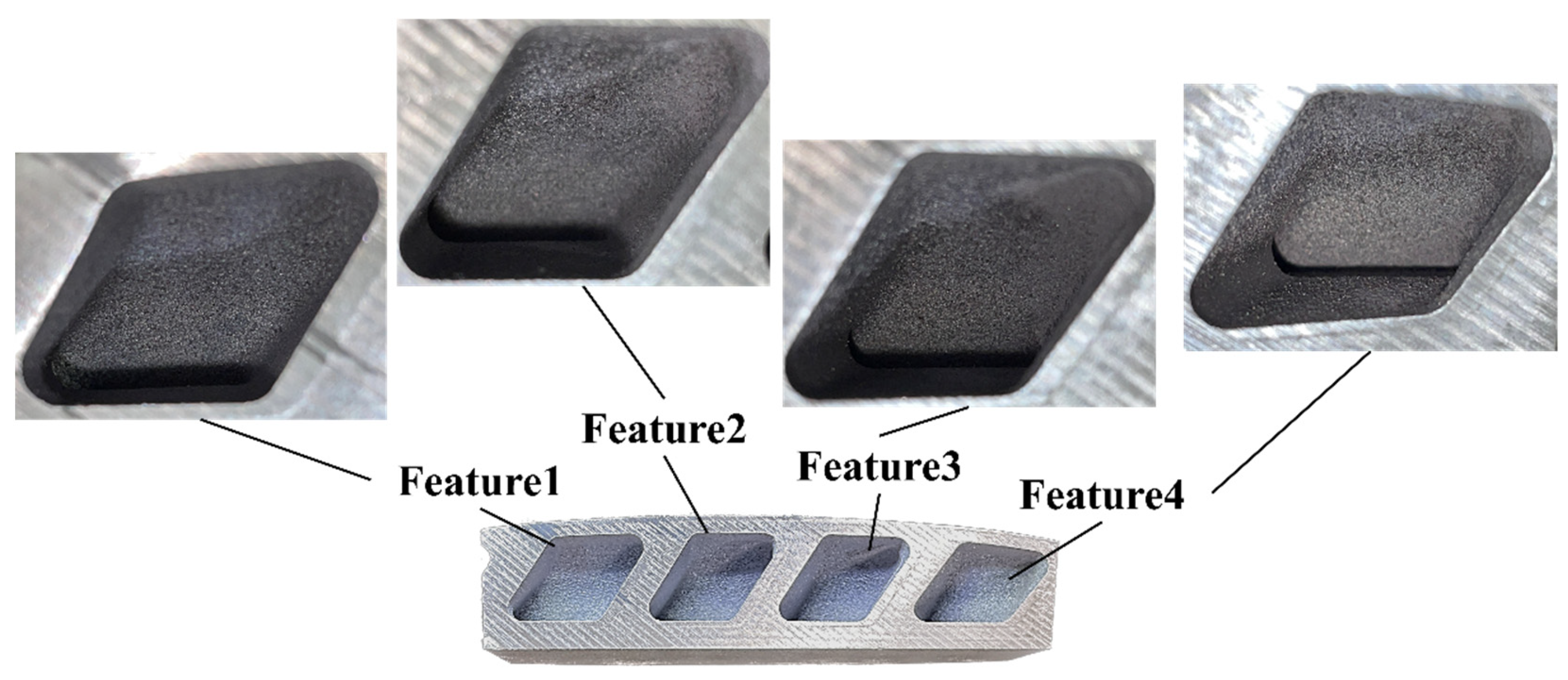
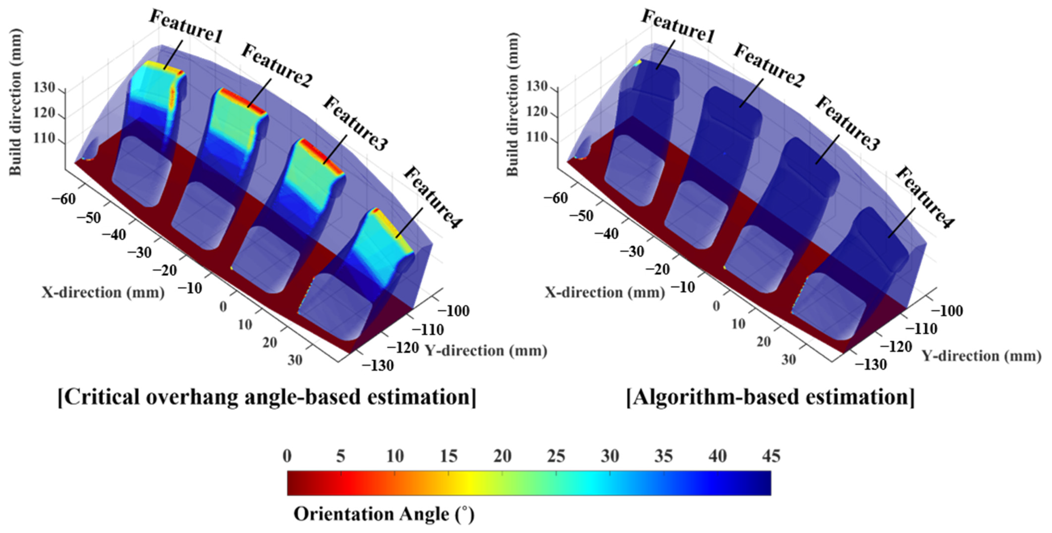
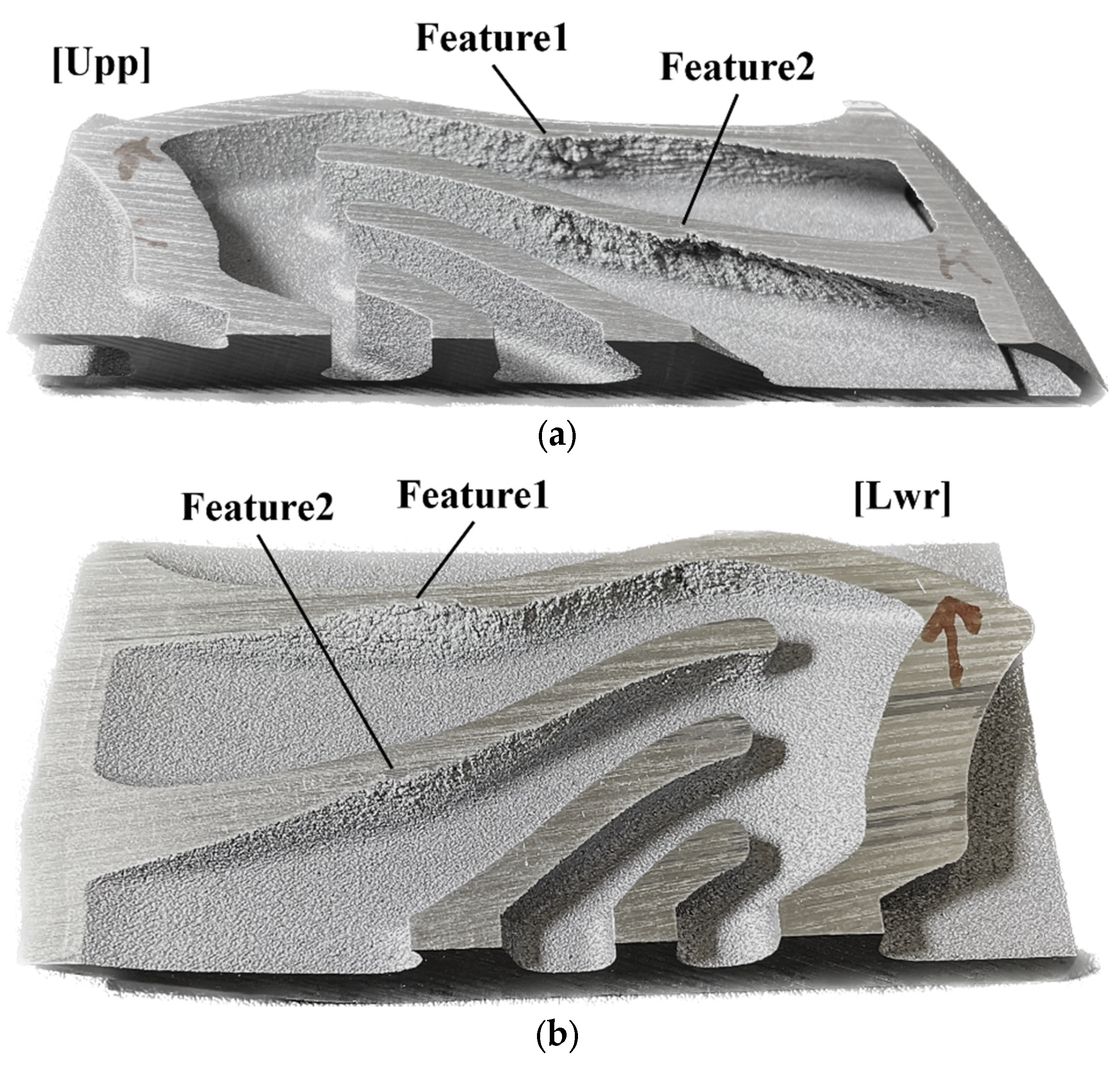
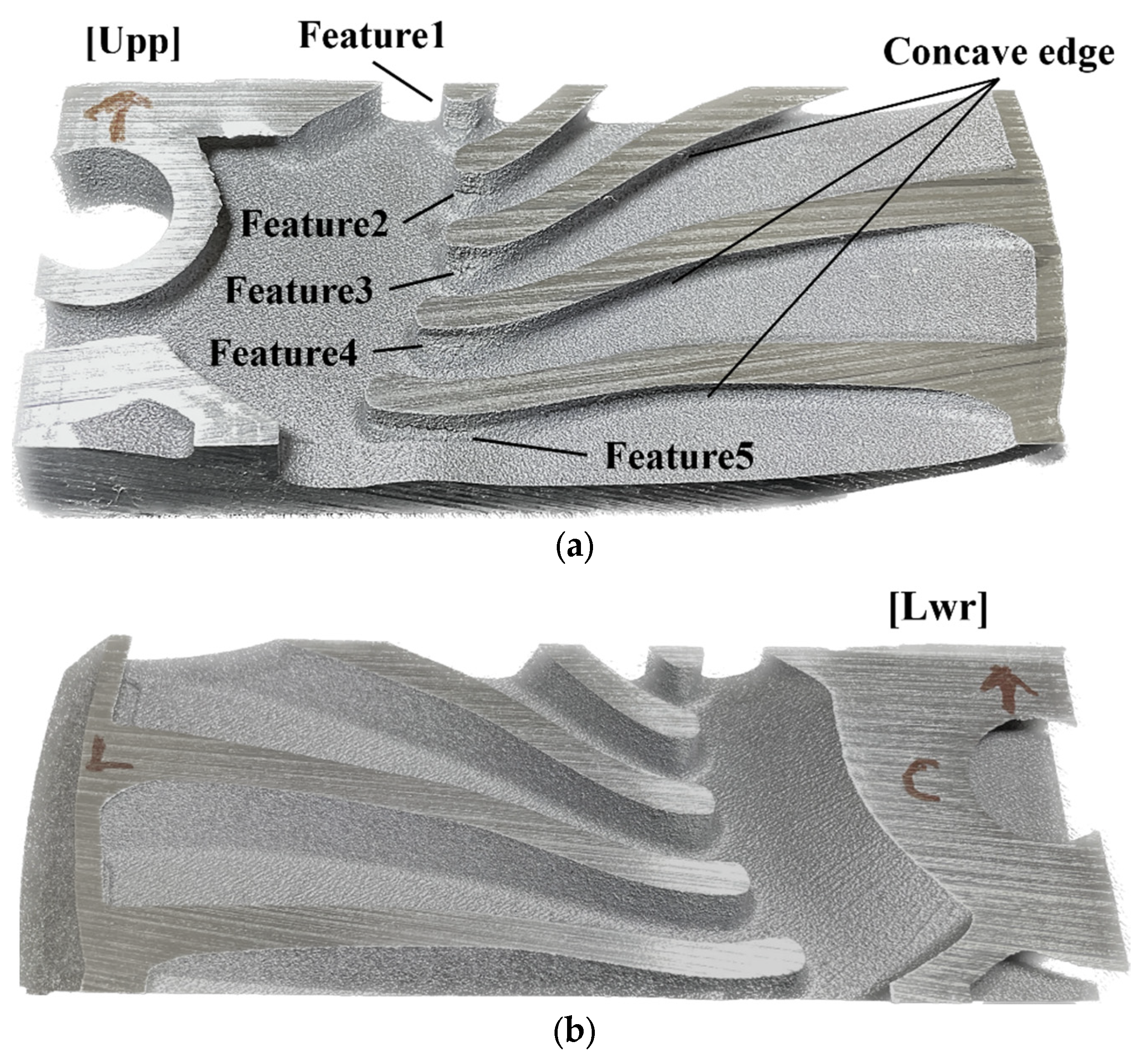
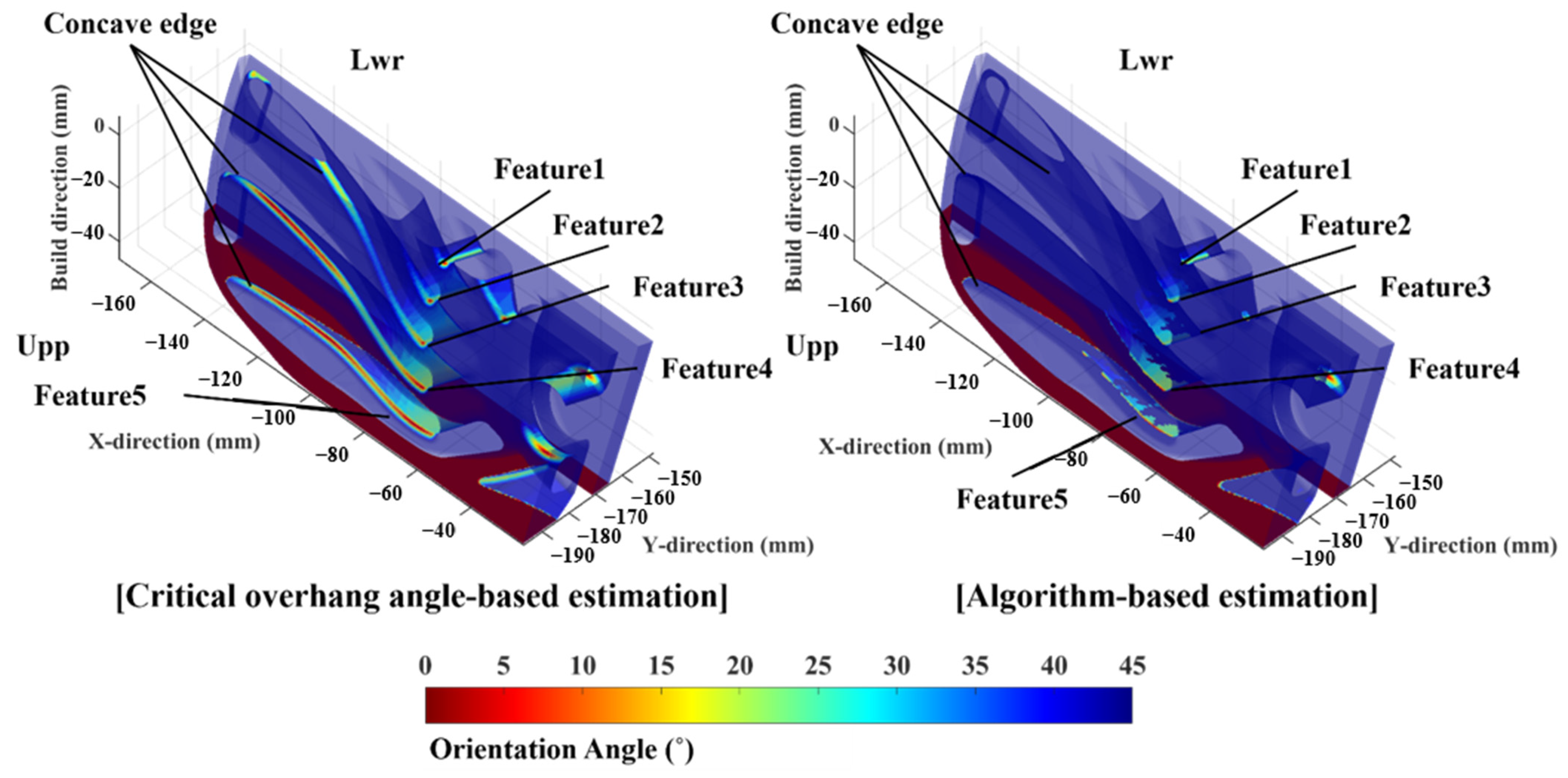
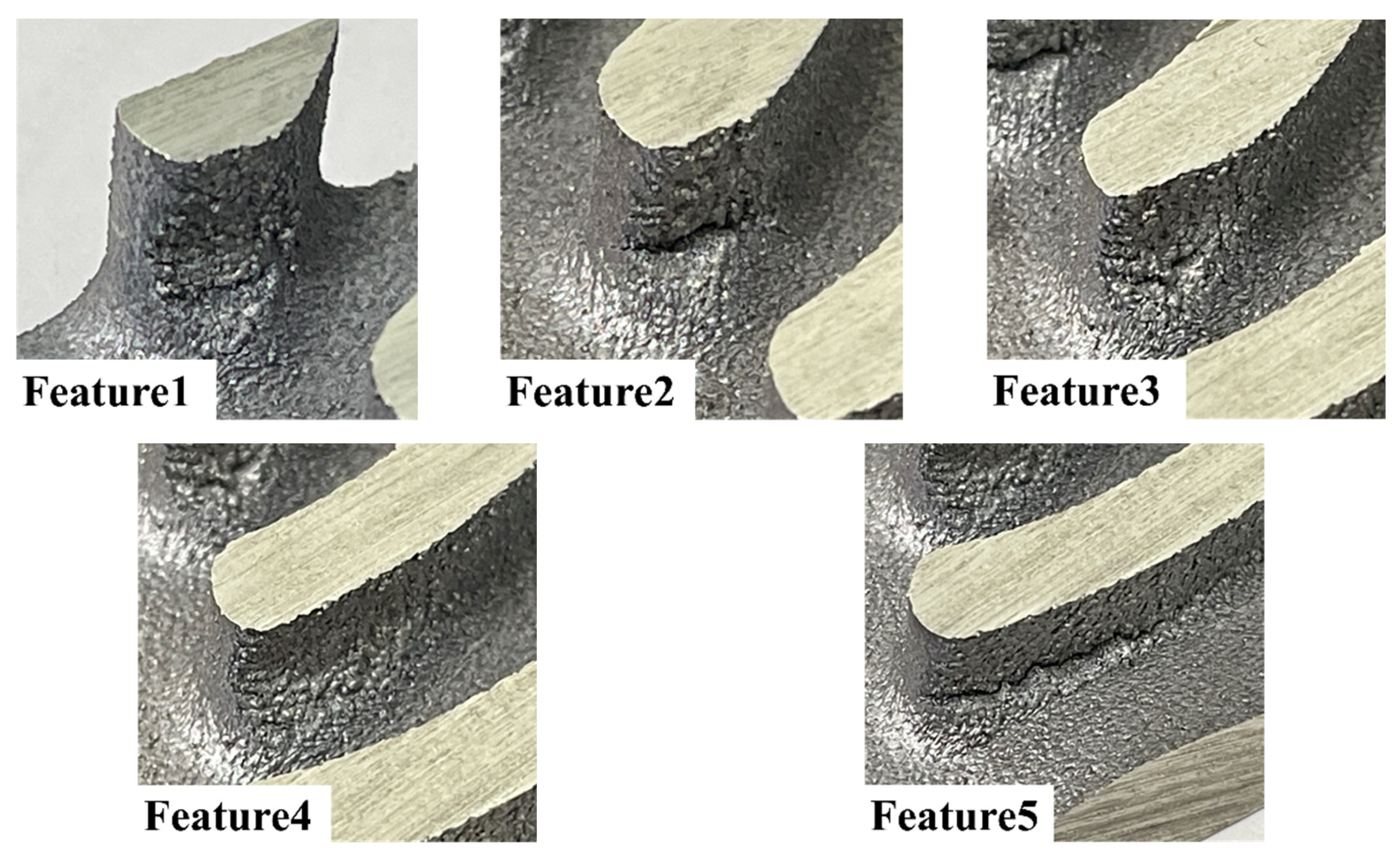
4.1. Sample 1
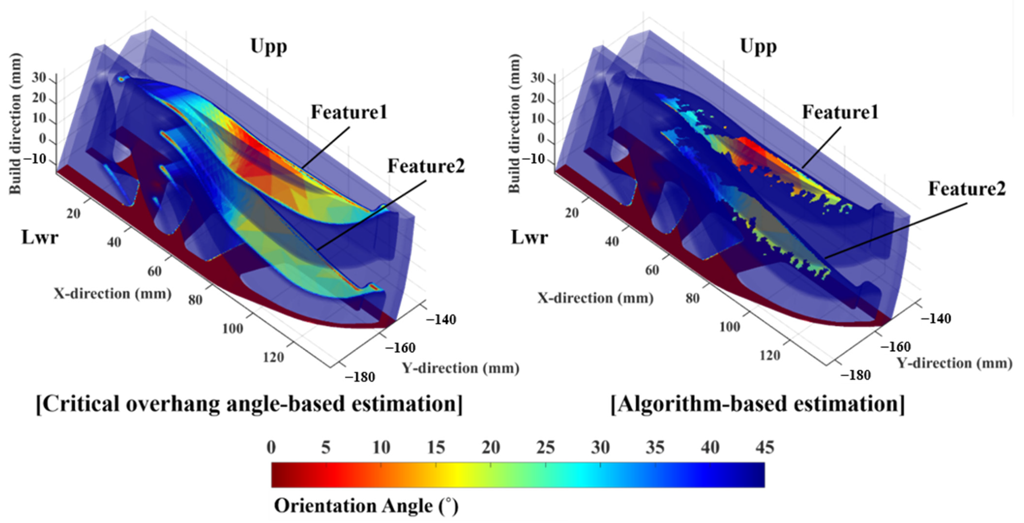
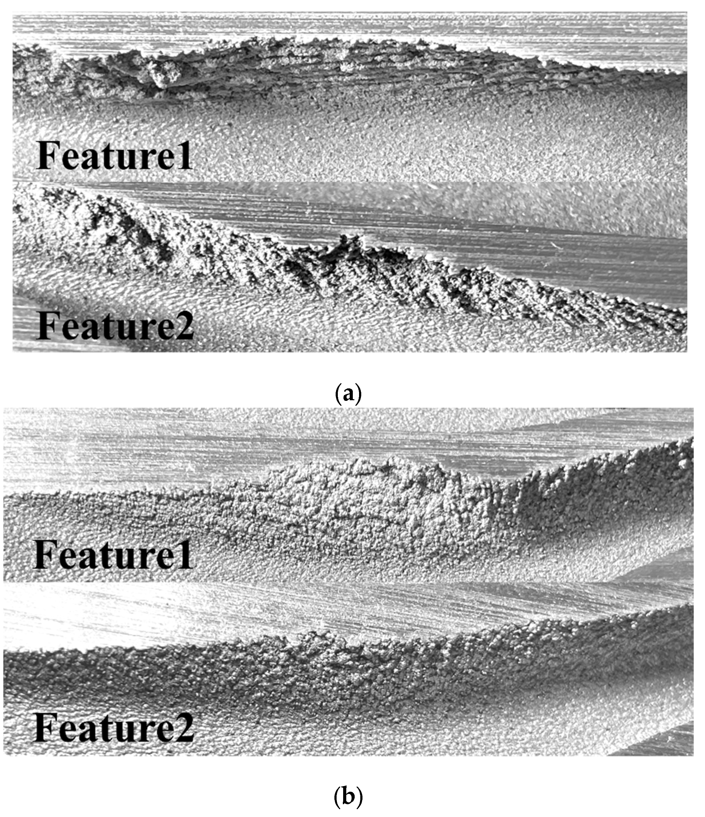
4.2. Sample 2
4.3. Sample 3
5. Conclusions
Author Contributions
Funding
Institutional Review Board Statement
Informed Consent Statement
Data Availability Statement
Acknowledgments
Conflicts of Interest
References
- Kaur, I.; Singh, P. State-of-the-art in heat exchanger additive manufacturing. Int. J. Heat Mass Transf. 2021, 178, 121600. [Google Scholar] [CrossRef]
- Gibson, I.; Rosen, D.; Stucker, B. Powder bed fusion processes. In Additive Manufacturing Technologies; Springer: New York, NY, USA, 2015; pp. 107–145. [Google Scholar]
- Stimpson, C.K.; Snyder, J.C.; Thole, K.A.; Mongillo, D. Scaling roughness effects on pressure loss and heat transfer of additively manufactured channels. J. Turbomach. 2017, 139, 021003. [Google Scholar] [CrossRef]
- Feng, S.; Kamat, A.M.; Sabooni, S.; Pei, Y. Experimental and numerical investigation of the origin of surface roughness in laser powder bed fused overhang regions. Virtual Phys. Prototyp. 2021, 16 (Suppl S1), S66–S84. [Google Scholar] [CrossRef]
- Çelik, A.; Tekoğlu, E.; Yasa, E.; Sönmez, M.Ş. Contact-Free Support Structures for the Direct Metal Laser Melting Process. Materials 2022, 15, 3765. [Google Scholar] [CrossRef]
- Han, Q.; Gu, H.; Soe, S.; Setchi, R.; Lacan, F.; Hill, J. Manufacturability of AlSi10Mg overhang structures fabricated by laser powder bed fusion. Mater. Des. 2018, 160, 1080–1095. [Google Scholar] [CrossRef]
- Ameen, W.; Al-Ahmari, A.; Mohammed, M.K. Self-supporting overhang structures produced by additive manufacturing through electron beam melting. Int. J. Adv. Manuf. Technol. 2019, 104, 2215–2232. [Google Scholar] [CrossRef]
- Zhou, M.; Liu, Y.; Lin, Z. Topology optimization of thermal conductive support structures for laser additive manufacturing. Comput. Methods Appl. Mech. Eng. 2019, 353, 24–43. [Google Scholar] [CrossRef]
- Solyaev, Y.; Rabinskiy, L.; Tokmakov, D. Overmelting and closing of thin horizontal channels in AlSi10Mg samples obtained by selective laser melting. Addit. Manuf. 2019, 30, 100847. [Google Scholar] [CrossRef]
- Khorasani, M.; Ghasemi, A.; Leary, M.; Sharabian, E.; Cordova, L.; Gibson, I.; Downing, D.; Bateman, S.; Brandt, M.; Rolfe, B. The effect of absorption ratio on meltpool features in laser-based powder bed fusion of IN718. Opt. Laser Technol. 2022, 153, 108263. [Google Scholar] [CrossRef]
- Wu, F.; Sun, Z.; Chen, W.; Liang, Z. The Effects of Overhang Forming Direction on Thermal Behaviors during Additive Manufacturing Ti-6Al-4V Alloy. Materials 2021, 14, 3749. [Google Scholar] [CrossRef]
- Biedermann, M.; Beutler, P.; Meboldt, M. Automated design of additive manufactured flow components with consideration of overhang constraint. Addit. Manuf. 2021, 46, 102119. [Google Scholar] [CrossRef]
- Ravalji, J.M.; Raval, S.J. Review of quality issues and mitigation strategies for metal powder bed fusion. Rapid Prototyp. J. 2022. ahead of print. [Google Scholar] [CrossRef]
- Giganto, S.; Martínez-Pellitero, S.; Cuesta, E.; Zapico, P.; Barreiro, J. Proposal of design rules for improving the accuracy of selective laser melting (SLM) manufacturing using benchmarks parts. Rapid Prototyp. J. 2022, 28, 1129–1143. [Google Scholar] [CrossRef]
- Linares, J.M.; Chaves-Jacob, J.; Lopez, Q.; Sprauel, J.M. Fatigue life optimization for 17-4Ph steel produced by selective laser melting. Rapid Prototyp. J. 2022, 28, 1182–1192. [Google Scholar] [CrossRef]
- Wang, Z.; Zhang, Y.; Tan, S.; Ding, L.; Bernard, A. Support point determination for support structure design in additive manufacturing. Addit. Manuf. 2021, 47, 102341. [Google Scholar] [CrossRef]
- Huang, J.; Kwok, T.H.; Zhou, C.; Xu, W. Surfel convolutional neural network for support detection in additive manufacturing. Int. J. Adv. Manuf. Technol. 2019, 105, 3593–3604. [Google Scholar] [CrossRef]
- Vora, P.; Mumtaz, K.; Todd, I.; Hopkinson, N. AlSi12 in-situ alloy formation and residual stress reduction using anchorless selective laser melting. Addit. Manuf. 2015, 7, 12–19. [Google Scholar] [CrossRef] [Green Version]
- Meng, L.; Zhang, W.; Quan, D.; Shi, G.; Tang, L.; Hou, Y.; Breitkopf, P.; Zhu, J.; Gao, T. From topology optimization design to additive manufacturing: Today’s success and tomorrow’s roadmap. Arch. Comput. Methods Eng. 2020, 27, 805–830. [Google Scholar] [CrossRef]
- Yang, T.; Liu, T.; Liao, W.; Wei, H.; Zhang, C.; Chen, X.; Zhang, K. Effect of processing parameters on overhanging surface roughness during laser powder bed fusion of AlSi10Mg. J. Manuf. Process. 2021, 61, 440–453. [Google Scholar] [CrossRef]
- Kuo, Y.H.; Cheng, C.C. Self-supporting structure design for additive manufacturing by using a logistic aggregate function. Struct. Multidiscip. Optim. 2019, 60, 1109–1121. [Google Scholar] [CrossRef]
- Schnittker, K.; Arrieta, E.; Jimenez, X.; Espalin, D.; Wicker, R.B.; Roberson, D.A. Integrating digital image correlation in mechanical testing for the materials characterization of big area additive manufacturing feedstock. Addit. Manuf. 2019, 26, 129–137. [Google Scholar] [CrossRef]
- AlMangour, B.; Yang, J.M. Improving the surface quality and mechanical properties by shot-peening of 17-4 stainless steel fabricated by additive manufacturing. Mater. Des. 2016, 110, 914–924. [Google Scholar] [CrossRef]
- Langelaar, M. Topology optimization of 3D self-supporting structures for additive manufacturing. Addit. Manuf. 2016, 12, 60–70. [Google Scholar] [CrossRef] [Green Version]
- Matos, M.A.; Rocha, A.M.A.; Pereira, A.I. Improving additive manufacturing performance by build orientation optimization. Int. J. Adv. Manuf. Technol. 2020, 107, 1993–2005. [Google Scholar] [CrossRef]


| Properties | 25 °C | 90 °C |
|---|---|---|
| Density (g/cm3) | 2.67 | |
| Specific heat (J/g K) | 0.913 | 0.901 |
| Thermal conductivity (W/m∙K) | 136.155 | 137.385 |
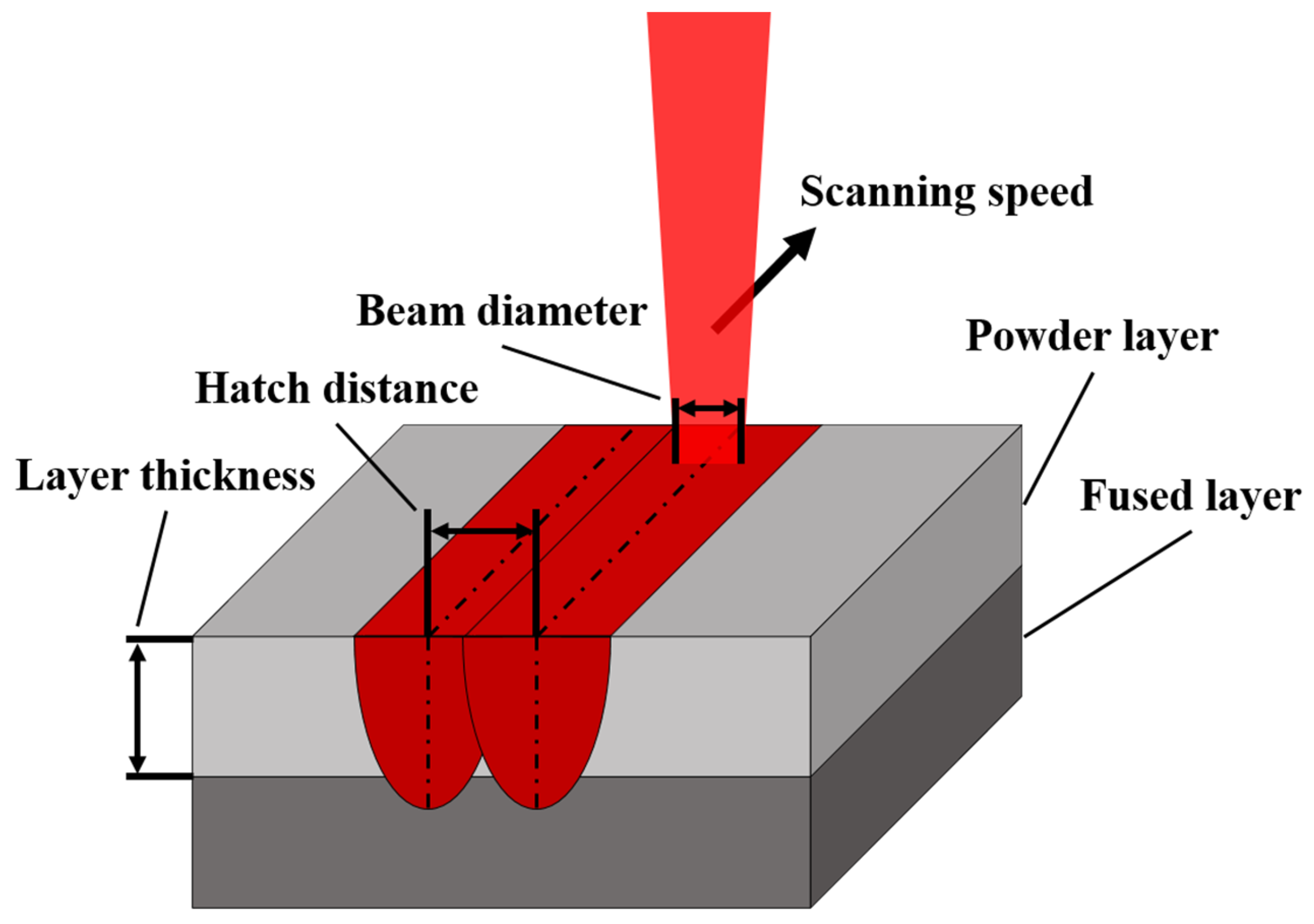
| Operation Parameter | Infill | Contour |
|---|---|---|
| Power (W) | 370 | 370 |
| Scanning speed (mm/s) | 1300 | 1300 |
| Beam diameter (mm) | 0.11 | 0.075 |
| Hatch distance (mm) | 0.14 | |
| Layer thickness (mm) | 0.06 | |
| Sample 1 | Sample 2 | Sample 3 | |
|---|---|---|---|
| Number of facet elements | 166,932 | 319,076 | 395,066 |
| Number of iterations | 101 | 53 | 92 |
| Surface area (m2) | 0.0189 | 0.0361 | 0.0447 |
| Processing time (s) | 441 | 1088 | 1862 |
Disclaimer/Publisher’s Note: The statements, opinions and data contained in all publications are solely those of the individual author(s) and contributor(s) and not of MDPI and/or the editor(s). MDPI and/or the editor(s) disclaim responsibility for any injury to people or property resulting from any ideas, methods, instructions or products referred to in the content. |
© 2023 by the authors. Licensee MDPI, Basel, Switzerland. This article is an open access article distributed under the terms and conditions of the Creative Commons Attribution (CC BY) license (https://creativecommons.org/licenses/by/4.0/).
Share and Cite
Lee, S.-Y.; Lee, J.-W.; Yang, M.-S.; Kim, D.-H.; Jung, H.-G.; Ko, D.-C.; Kim, K.-W. Facet Connectivity-Based Estimation Algorithm for Manufacturability of Supportless Parts Fabricated via LPBF. Materials 2023, 16, 1039. https://0-doi-org.brum.beds.ac.uk/10.3390/ma16031039
Lee S-Y, Lee J-W, Yang M-S, Kim D-H, Jung H-G, Ko D-C, Kim K-W. Facet Connectivity-Based Estimation Algorithm for Manufacturability of Supportless Parts Fabricated via LPBF. Materials. 2023; 16(3):1039. https://0-doi-org.brum.beds.ac.uk/10.3390/ma16031039
Chicago/Turabian StyleLee, Seung-Yeop, Jae-Wook Lee, Min-Seok Yang, Da-Hye Kim, Hyun-Gug Jung, Dae-Cheol Ko, and Kun-Woo Kim. 2023. "Facet Connectivity-Based Estimation Algorithm for Manufacturability of Supportless Parts Fabricated via LPBF" Materials 16, no. 3: 1039. https://0-doi-org.brum.beds.ac.uk/10.3390/ma16031039