AI-Based Posture Control Algorithm for a 7-DOF Robot Manipulator

Abstract

With the rapid development of artificial intelligence (AI) technology and an increasing demand for redundant robotic systems, robot control systems are becoming increasingly complex. Although forward kinematics (FK) and inverse kinematics (IK) equations have been used as basic and perfect solutions for robot posture control, both equations have a significant drawback. When a robotic system is highly nonlinear, it is difficult or impossible to derive both the equations. In this paper, we propose a new method that can replace both the FK and IK equations of a seven-degrees-of-freedom (7-DOF) robot manipulator. This method is based on reinforcement learning (RL) and artificial neural networks (ANN) for supervised learning (SL). RL was used to acquire training datasets consisting of six posture data in Cartesian space and seven motor angle data in joint space. The ANN is used to make the discrete training data continuous, which implies that the trained ANN infers any new data. Qualitative and quantitative evaluations of the proposed method were performed through computer simulation. The results show that the proposed method is sufficient to control the robot manipulator as efficiently as the IK equation.

1. Introduction

A robot manipulator is a generally and widely used robot, which is also called an industrial robot, serial robot, or robotic arm. Most robot manipulators are used in industrial fields for practical and automated purposes such as welding, cutting, picking, and placing objects. There are various types of robot manipulators, depending on the number of joints and direction of assembly.

Robot manipulators are categorized into three groups according to the number of joints: less than six degrees-of-freedom (6-DOF), 6-DOF, and more than 6-DOF. The reason for categorizing by 6-DOF is that at least six parameters are required to describe the motion of an object in three-dimensional (3D) space. The first group consists of robot manipulators using fewer than six joints, which cannot express the entire 6-DOF information and have limited motions. A 2-DOF robot can only control the ($x$, $y$) position; for example, Elsis et al., (2021) [1] and Urrea et al., (2021) [2] adopted RR and RP types of 2-DOF robots, respectively. R and P indicate revolute and prismatic, respectively. A 3-DOF robot can control either ($x$, $y$, $z$) or ($x$, $y$, $\alpha$) posture; for example, Martín et al., (2000) [3] and Azizi (2020) [4] adopted Zebra ZERO of RRR type and three variants of RRR, RRP (Stanford arm), and RPR type, respectively. A 4-DOF robot can control ($x$, $y$, $z$, $\alpha$) posture; for example, Ram et al., (2019) [5] and Boschetti (2020) [6] adopted RRRR and Cobra 600 ©Adept Technology of RRPR type, respectively. The second group consists of robot manipulators using six joints. This group can express all the DOF in the real world. This group has seen the most development; for example, STEP SD 700 [7], Stanford MT-ARM [8], UR5 ©Universal Robots [9], KUKA-kr ©KUKA [10], M710i ©FANUC [11], ABB IRB 1600 [12], and Viper 650 ©Adept Technology [6] are being employed in various research projects. However, this group has only one solution per posture and singular points. The third group comprises robot manipulators that use more than six joints, also called redundant robots. This group has diverse solutions per posture, and the movement of the robot manipulator appears visually flexible; for example, Baxter arm [13], LWA 4D ©Schunk [14], LBR iiwa 7 R800 ©KUKA [15], SUNGUR 370 [16], Cyton Gamma 300 [17], WAM arm © Barrett Technology [18], Sawyer ©Rethink Robotics [19], and SARCOS Master Robot Arm [20] are 7-DOF. There is an increasing demand for redundant robot manipulators for improved technologies such as flexible operation and/or human-level performance. However, the development of redundant robotic manipulators is challenging. This group has highly nonlinear systems that are extremely difficult to analyze and control. For the developer, designing and programming them is a difficult task.

The operation and control of robot manipulators involve many aspects, such as posture control (position and orientation control) [21,22,23], dynamic control (velocity-related control) [24], torque control (acceleration-related control) [25], and path planning [26,27,28].

Among them, posture control is a fundamental and essential topic because its control error has a sequential effect on the following control system. To control the posture of the robot manipulator, developers require inverse kinematic equations. However, inverse kinematic (IK) equations, particularly for redundant robots, are difficult or impossible to derive. For example, the joint space parameters of the $n$-DOF system should be derived from position $x$ expressed as $x=\cos \left({\theta }_1+\cdots +{\theta }_n\right)$, from which it is very difficult to derive the equations explicitly. Moreover, even if an IK equation is derived for a particular robot manipulator, the equation must be re-derived if the kinematic properties change, e.g., dynamic changes in the transformation and several swarm robot systems. Furthermore, redundant robot systems have multiple control solutions per posture. For these reasons, there is a need for an adaptive and scalable algorithm to be used in place of the inverse kinematic equations.

There have been many posture control methods for deriving the kinematic equations of 7-DOF robot manipulators: analytical methods, numerical methods, and AI-based methods.

The analytical method is a general approach. In this method, the characteristics of link size, joint angle, and assembly direction are used to derive a mathematical equation, known as the IK equation. Several attempts have been made to derive the IK equations for a 7-DOF articulated robot. Wang et al., (2010) proposed a closed-loop inverse kinematics (CLIK) algorithm for position control and redundancy resolution [29]. Gong et al., (2019) proposed analytical IK for KUKA LBR iiwa 7-DOF redundant manipulator [30]. The IK solution groups three control parameters: elbow (first, second, and third joints), arm (fourth joint), and wrist (fifth, sixth, and seventh joints). Whenever controlling the 7-DOF robot, they solve and aggregate the results of two 3-DOF IK and a 1-DOF revolute joint. In both of them, the simulation results showed good performance because the analytical method was an exact solution. However, the IK equations must be rederived for different robots according to their structure and shape. This implies poor compatibility of the analytical method.

Numerical methods typically use optimization approaches to minimize the defined loss function. Huang et al., (2012) employed a particle swarm optimization (PSO) for solving the IK equation of 7-DOF robotic manipulators [31]. The PSO algorithm has a multitude of optimizers, which find the joint space parameters with a minimum posture error. However, the PSO algorithm is at risk of finding local convergence rather than global convergence. To solve this problem, Dereli et al., (2019) developed a quantum-behaved particle swarm (QPSO) algorithm for 7-DOF articulated robot control [32]. QPSO makes the particles more dynamic, with wave function instead of position and velocity variables in PSO. This study sets the end-effector position as a particle and optimizes the perturbation movement using the Euclidean distance. However, the QPOS does not consider the orientation of the end effector, which affects the limits of postural control.

AI-based methods are currently a major research topic in robotics. This method approximates a function based on desired data. There have been some prior efforts to replace the IK of robot manipulators with artificial intelligence (AI). Jiménez-López et al., (2021) proposed a method for modeling a 3-DOF PUMA robot using a neural network to solve the inverse kinematic problem [33]. With the ANN composed of three hidden layers with 25 neurons per layer, they calculated the IK anywhere in the movement-space of the robot with low effective errors. However, the derivation of the inverse kinematic equations for 3-DOF robots is possible with an analytical approach, which gives an even more exact solution. Kramar et al., (2022) proposed an ANN architecture having 8 hidden layers with 30 or 60 neurons per layer to solve the IK problem of the 6-DOF anthropomorphic manipulator of robot SAR-401 [34]. The proposed ANN showed high accuracy in the simulation results but required expensive computational resources and costs due to many layers and neurons. There are some existing studies targeting 7-DOF robot manipulators, such as this paper. Bretan et al., (2019) employed an artificial neural network (ANN) to solve inverse kinematic problems for a 7-DOF Sawyer articulated robot [19]. They used collaborative network training with a multi-ANN having 3 hidden layers, each with 200 nodes, for position control. The results of ANNs were satisfactory, but the robot moved in a very narrow range of the workspace even when many nodes were set. The most essential feature of the ANN method is training data with labels, which were not provided. In addition, this ANN-based method takes a long time for computation and requires a large amount of memory compared with previous methods. Peters et al., (2007) applied reinforcement learning (RL) to solve inverse kinematic problems for a 7-DOF SARCOS articulated robot [20]. This research introduced the reward-weighted regression method and conducted experiments using a real robot. The experimental results were successful; however, the learning time was slow. The 7-DOF required approximately 6 h of training time, and the 3-DOF required 2 h. Consequently, they are difficult to use in practical control algorithms. Recently, AI-based methods have shown remarkable research achievements, so we briefly introduce more research cases on AI algorithms to other applications. Azizi (2020) adopted a genetic algorithm (GA) and ANN for kinematics synthesis of three 3-DOF robot arms: RRR, RPR, and Stanford arm [4]. GA and ANN are used to find optimal design parameters such as link lengths, assembly directions, and so on. Giorgio et al., (2020) proposed an AI path-finding algorithm to control a robot with an optimized trajectory with collision avoidance applied [12]. Chen et al., (2021) proposed a manipulator control system based on an AI wearable acceleration sensor to realize the remote grasping operation [21]. Lim et al., (2021) proposed a CNN model-based control algorithm for a 6-DOF robotic arm directly controlled by brainwaves, also known as electroencephalogram (EEG) signals [28]. A CNN model takes an input of an EGG signal and classifies the output into one of eight mental commands (forward, backward, up, down, left, right, open, close).

In this study, a new AI-based posture control algorithm for a 7-DOF robot manipulator is presented. The proposed algorithm is based on RL and ANN. The RL-based posture control algorithm is used rather than the forward kinematics (FK) equation to generate the training data for the ANN-based posture control algorithm. The ANN approximates an IK function for posture control. The results of the proposed method satisfied the limit of the control error and were sufficiently good to be used for the posture control of the 7-DOF robot manipulator. The entire development procedure was simulated using MATLAB software.

The proposed method has three advantages: (1) learning from scratch, (2) learning faster than online learning, and (3) compatibility with other robotic systems. First, learning from scratch was feasible. This is because RL and ANN complement mutual drawbacks while considering their respective strengths. RL learns optimal policies, but policy data are discrete. An ANN is a good function approximator, but cannot be trained without any training data. Therefore, RL generates training data for posture control, and ANN approximates the training data and controls the posture of the robot manipulator. Second, the proposed method was faster than the online method. Online learning is synchronously updated. There should be interaction delays between the agent and environment. However, the offline method works independently. Therefore, there are no interaction delays, which shorten the learning time. Third, the proposed method can be applied to any type of robot manipulator, regardless of the DOFs and structures. Since RL training collects training data based on interactions, an ANN can approximate any property of the data. As a proof of concept and precedence study, we applied this algorithm to a heterogeneous quadrupedal robotic system [35]. We derived IK equations for a quadrupedal robot to balance against an arbitrarily and dynamically tilted ground. Although the IK equation for a quadrupedal robot is laborious, it can be derived with effort. However, finding the closed-form IK equation for a 7-DOF manipulator is impossible because it is a more complex nonlinear system. Therefore, this step-up study shows that our algorithm can be applied to a wide variety of robots.

The rest of the paper is organized as follows. Section 2 explains the basic knowledge according to the robot manipulator and AI algorithms. Section 3 introduces the system of the 7-DOF robot manipulator. Section 4 and Section 5 show specific developments in AI-based algorithms, RL, and ANN. In Section 6, experimental evaluations of posture control are presented qualitatively and quantitatively. Section 7 concludes the paper and presents the prospects for future work. The Appendix A, Appendix B and Appendix C covers detailed learning implementations and derivation procedures.

2. Background

For a better understanding of the AI-based posture control algorithm for the 7-DOF robot manipulator, in this section, we explain the kinematic analysis and AI algorithm.

2.1. Kinematic Analysis

Kinematic analysis studies the static relationship between the joint angles of a robot manipulator and the robot posture of an end effector. The joint angles ($\theta$) are joint space parameters: angles for $n$-DOFs (${\theta }_1$, …, ${\theta }_n$). The robot’s posture ($q$) consists of Cartesian space parameters: position ($x$, $y$, $z$) and orientation ($\alpha$, $\beta$, $\gamma$). The relationship between the robot posture and joint angles is called IK analysis, and the reverse is called FK analysis.

The IK equation ($f_{IK}$) is an intuitive control approach for users. For example, if a user wants to pick up a box using a robot, he/she is more accustomed to instructing the desired posture ($q$) of the end effector toward the box rather than the set of angles ($\theta$) of the motors. The IK equation transforms the end-effector posture as an input into joint angles as the output, as expressed in Equation (1):

$$\theta =f_{IK}\left(q\right).$$

(1)

However, it is difficult to derive the IK equation for a 7-DOF robot manipulator. The joint space parameters are implicit in trigonometry, for example, $x=\cos \left({\theta }_1+{\theta }_2\right)$. Therefore, it is difficult to specify joint angles explicitly using Cartesian space parameters. Another issue is compatibility; even if an IK equation is derived for a particular robot manipulator, the equation must be derived again if the kinematic properties change.

The FK equation ($f_{FK}$) can be derived for any robotic manipulator. The FK equation transforms the joint angles as inputs into the end-effector pose as the output in Equation (2):

$$q=f_{FK}\left(\mathsf{\theta }\right).$$

(2)

If training and experiments are performed using a real robot, there is no need to derive the FK equation.

2.2. Artificial Inteligence Algorithm

The AI algorithm includes RL and ANN for supervised learning. Typically, RL is used to determine the optimal policy, and an ANN is used for classification or regression.

2.2.1. Reinforcement Learning

RL is an interaction-based learning algorithm between an agent and environment [36,37,38]. The agent is the subject of the learning system, which learns the optimal behavior for each state. The environment is the surroundings of the learning system, and it provides states and rewards to the agent.

RL parameters consist of state ($s$), action ($a$), policy ($\pi$), and reward ($r$). State $s$ represents the current situation between the agent and the environment. Action $a$ changes the current state to a next particular state. The policy $\pi$ is a tuple of states and actions. Reward r determines whether a particular action in its current state is an appropriate choice.

Generalized policy iteration (GPI) is an update process in RL and is divided into policy evaluation and policy improvement. Policy evaluation predicts the near future (next state), and policy improvement optimizes the current behavior to the appropriate behavior (next policy). The GPI iterates policy evaluation and policy improvement until the agent finds the optimal policy (${\pi }^{\ast }$) for the target state.

2.2.2. Artificial Neural Network for Supervised Learning

The ANN for supervised learning is a learning algorithm that approximates the relationship between the input and output of training data for classification or regression [39]. Training an ANN involves adjusting the weights and biases of the ANN with respect to the training data. To train, the ANN performs forward and backward propagation.

Forward propagation computes the prediction value. To obtain the prediction value, the training input data are fed into an ANN structure consisting of an input layer, hidden layers, and output layer. At each layer, the fed data compute the affine layer and activation function.

The predicted value from forward propagation is compared with the training output data labeled by a supervisor, and the compared error is called the loss function. If the ANN is not sufficiently trained, its prediction accuracy is poor, and the loss function has a large value. The ANN training should be directed toward reducing the loss function.

Backward propagation is a process that updates the weights and biases. The updates are conducted from the output to hidden and then to input layers. At each layer, the gradients for the weights and biases are computed from the partial derivatives of the loss function and chain rule. The gradients are then merged with original weights and biases, called updates.

Forward and backward propagation is repeated until the value of the loss function meets the target or the number of iterations reaches the maximum value.

3. 7-DOF Robot Manipulator

This section describes the configuration of the 7-DOF robot manipulator, the FK equation via the Denavit–Hartenberg (D–H) convention, and the posture control system.

3.1. Configuration of 7-DOF Robot Manipulator

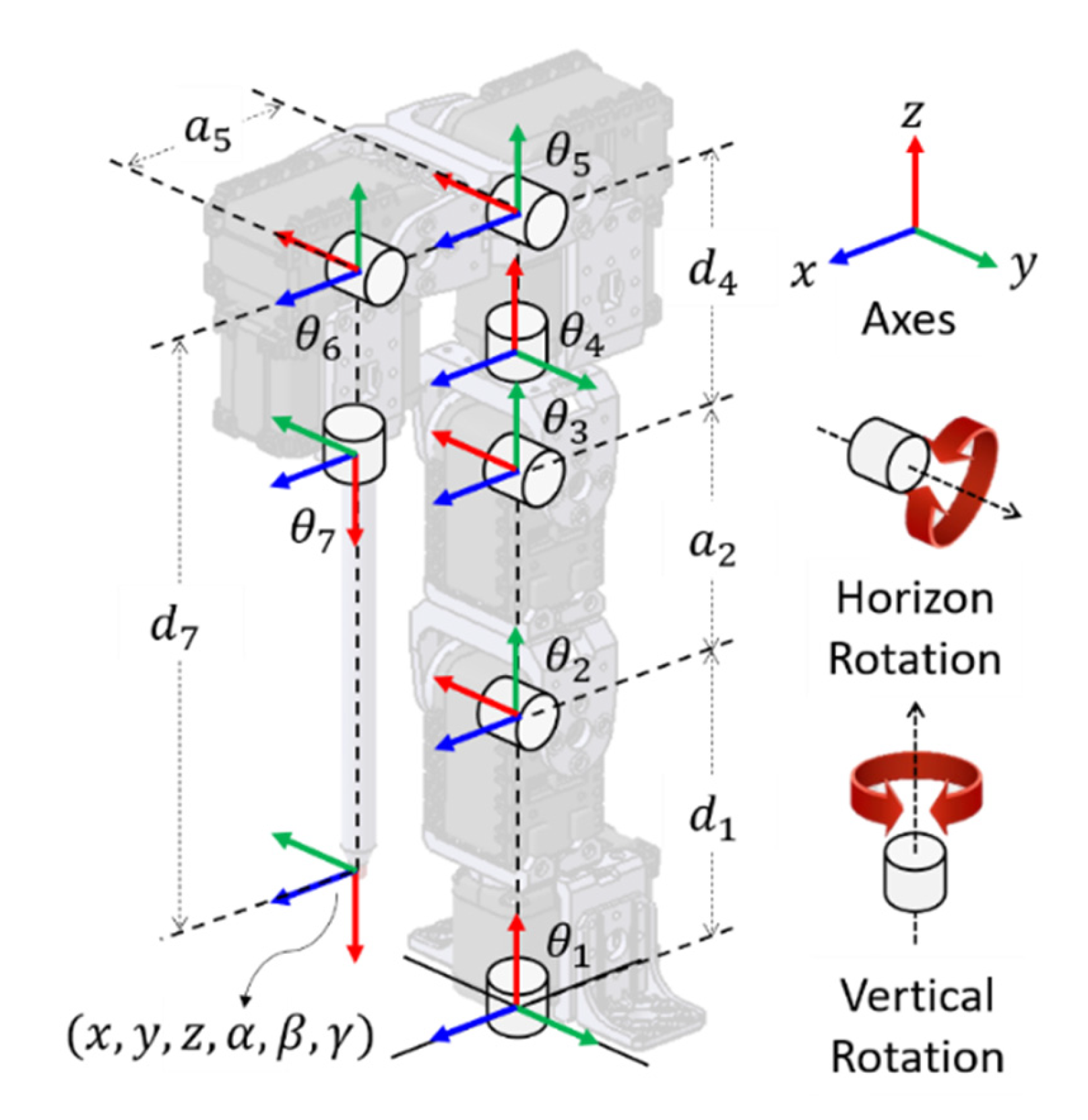
The 7-DOF robot manipulator was assembled using seven servo motors and a thin and long end effector, as depicted in Figure 1. The first servo motor was fixed to the ground. The other six servo motors were serially connected in two rotational directions. One rotates in the vertical (yaw) direction, using the first, fourth, and seventh motors. The other rotates in the horizontal (pitch) direction, using the second, third, fifth, and sixth motors. A thin and long end effector was attached at the end of the servo motor. The notations for the rotational directions and coordinate axes are shown in Figure 1.

3.2. Forward Kinematics Equation via D–H Convention

The FK equation for the 7-DOF robot was used for computer simulation. If RL training is performed with real 7-DOF robotic manipulators rather than computer simulations, the FK equation is no longer required. We took the computer simulation approach because it not only saves development time and money but also ensures the safety of robot components, even if it cannot fully cover all non-systematic errors.

The FK equation of the 7-DOF robot manipulator uses the information of the seven motor angles ${\theta }_1$, ${\theta }_2$, ${\theta }_3$, ${\theta }_4$, ${\theta }_5$, ${\theta }_6$, and ${\theta }_7$ as inputs and is derived as expressed in Equation (3):

$$f_{FK}={\displaystyle \prod }_{i=1}^7{H}_i^{i-1},$$

(3)

where $H_i^{i-1}$ is a D–H convention matrix of the $i$-th link where the 0-th link is a fixed base [40]. The D–H convention matrix transforms the coordinates from the previous $\left(i-1\right)$-th link to $i$-th link, as shown in Equations (4)–(8). The FK equation for the 7-DOF robot manipulator is obtained as follows:

$$H_i^{i-1}=R_z\left({\theta }_i\right)T_z\left(d_i\right)T_x\left(l_i\right)R_x\left({\omega }_i\right),$$

(4)

$$R_z\left({\theta }_i\right)=\left[\begin{array}{cc}\begin{array}{cc}\cos {\theta }_i& \sin {\theta }_i\\ -\sin {\theta }_i& \cos {\theta }_i\end{array}& \begin{array}{cc}0& 0\\ 0& 0\end{array}\\ \begin{array}{cc}0& 0\\ 0& 0\end{array}& \begin{array}{cc}1& 0\\ 0& 1\end{array}\end{array}\right],$$

(5)

$$T_z\left(d_i\right)=\left[\begin{array}{cc}\begin{array}{cc}1& 0\\ 0& 1\end{array}& \begin{array}{cc}0& 0\\ 0& 0\end{array}\\ \begin{array}{cc}0& 0\\ 0& 0\end{array}& \begin{array}{cc}1& d_i\\ 0& 1\end{array}\end{array}\right],$$

(6)

$$T_x\left(l_i\right)=\left[\begin{array}{cc}\begin{array}{cc}1& 0\\ 0& 1\end{array}& \begin{array}{cc}0& l_i\\ 0& 0\end{array}\\ \begin{array}{cc}0& 0\\ 0& 0\end{array}& \begin{array}{cc}1& 0\\ 0& 1\end{array}\end{array}\right],$$

(7)

$$R_x\left({\omega }_i\right)=\left[\begin{array}{cc}\begin{array}{cc}1& 0\\ 0& \cos {\omega }_i\end{array}& \begin{array}{cc}0& 0\\ \sin {\omega }_i& 0\end{array}\\ \begin{array}{cc}0& -\sin {\omega }_i\\ 0& 0\end{array}& \begin{array}{cc}\cos {\omega }_i& 0\\ 0& 1\end{array}\end{array}\right],$$

(8)

where $R_z$ and $T_z$ are the rotational and translational transition matrices with respect to the z-axis and $T_x$ and $R_x$ are the translational and rotational transition matrices with respect to the x-axis, respectively. There are four D–H parameters for the ith link: ${\theta }_i$ is the angle with respect to the z-axis, $d_i$ is the offset for the z-axis, $l_i$ is the length of the x-axis, and ${\omega }_i$ is the twist for the x-axis. These parameters are associated with structural connections. The D–H parameters of the 7-DOF robot manipulator are shown in Figure 1 and tabulated in

Table 1. Denavit–Hartenberg (D–H) parameters of the 7-DOF robot manipulator.

Link Number	$\mathbf{Angle}, {\mathit{\theta }}_{\mathit{i}}$$(°)$	$\mathbf{Offset}, {\mathit{d}}_{\mathit{i}} \left(\mathbf{mm}\right)$	$\mathbf{Length}, {\mathit{l}}_{\mathit{i}} \left(\mathbf{mm}\right)$	$\mathbf{Twist}, {\mathit{\omega }}_{\mathit{i}}$$(°)$	$\mathbf{Rotation} \mathbf{Range} (°)$
1	${\theta }_1$	81.50	0.00	90.00	−150.00	to	150.00
2	${\theta }_2$	0.00	67.50	0.00	−20.00	to	180.00
3	${\theta }_3$	0.00	0.00	−90.00	−180.00	to	20.00
4	${\theta }_4$	79.00	0.00	90.00	−150.00	to	150.00
5	${\theta }_5$	0.00	52.00	0.00	−20.00	to	90.00
6	${\theta }_6$	0.00	0.00	90.00	−20.00	to	90.00
7	${\theta }_7$	175.00	0.00	0.00	$\infty$, fully rotate

. For each link, only ${\theta }_i$ is variable, and the other parameters are constants.

According to Equation (3), the derived form of the FK equation by chained matrix multiplication is expressed in Equation (9):

$$f_{FK}=\left[\begin{array}{cc}\begin{array}{cc}{r}_{11}& r_{12}\\ r_{21}& r_{22}\end{array}& \begin{array}{cc}{r}_{13}& x\\ r_{23}& y\end{array}\\ \begin{array}{cc}{r}_{31}& r_{32}\\ 0& 0\end{array}& \begin{array}{cc}{r}_{33}& z\\ 0& 1\end{array}\end{array}\right],$$

(9)

where $x$, $y$, and $z$ are the positions of the end-effector that are explicitly expressed. However, orientations $\alpha$, $\beta$, and $\gamma$ were not directly represented. Hence, there are additional calculations with the five rotational elements, $r_{11}$, $r_{21}$, $r_{31}$, $r_{32}$, and $r_{33},$ using Equation (10), which is derived from the roll-pitch-yaw representation [40].

$$\alpha ={\tan }^{-1}\left(\frac{r_{32}}{r_{33}}\right), \beta ={\tan }^{-1}\left(\frac{r_{31}}{\sqrt{r_{11}^2+r_{21}^2}}\right), \gamma ={\tan }^{-1}\left(\frac{r_{21}}{r_{11}}\right).$$

(10)

The implementation of the FK equation is presented in Appendix A, where for each of the servo motors of the 7-DOF robot manipulator, $\theta =\left(0°,90°,-90°,0°,0°,0°,0°\right)$ and $q=\left(52 \mathrm{mm},y=0 \mathrm{mm},z=53 \mathrm{mm},\alpha =180°,\beta =0°,\gamma =0°\right)$, computed using Equations (3)–(10).

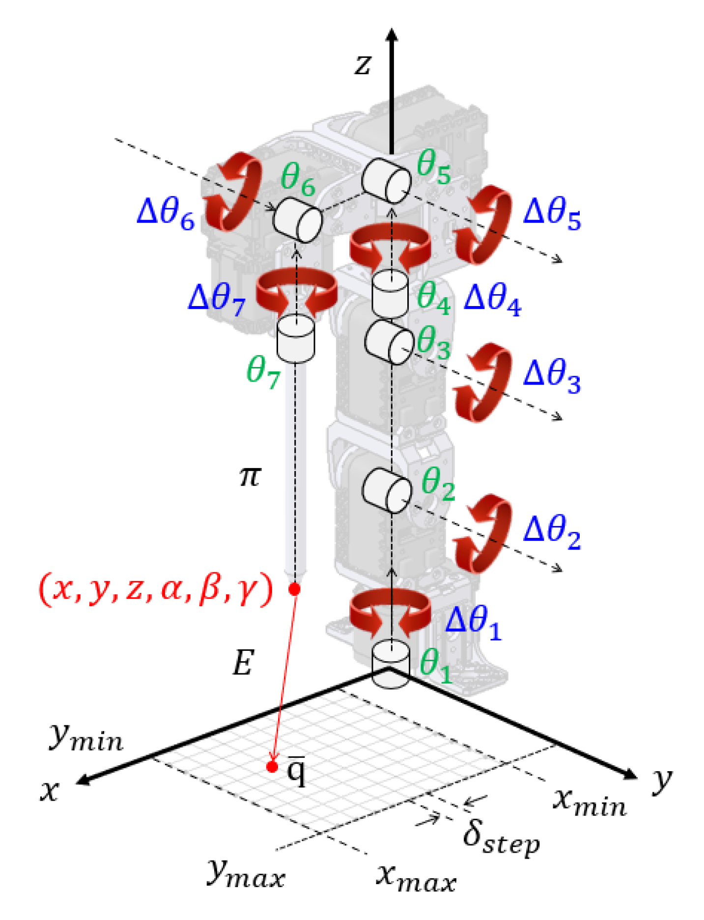
3.3. Posture Control System

The posture control system consists of a robot manipulator, RL, and an ANN, as shown in Figure 2. The generalized policy iteration (GPI) module in RL measures the end-effector posture ($q$) in the robot manipulator after receiving the trajectory ($\tau$) from the path-planning module. The path-planning module plans the initial posture and subsequent trajectory postures and outputs the sequence of postures. The GPI module computes and transmits the joint angles ($\theta$) of the servo motors while learning the optimal policy. After the training of the RL has been completed, the training data ($D$) are passed to the training session of the ANN. The training session trains the ANN and passes the weights ($W$) and biases ($b$) to the inference session after ANN training has been completed. The inference session performs postural control. If RL and ANN training are not complete owing to the trajectory, the training session signals the path-planning module to replan the trajectory path.

4. RL-Based Posture Control Algorithm

The RL-based posture control algorithm is used rather than the FK equation to generate training data for the ANN-based posture control algorithm. The development procedure of the RL-based posture control algorithm, its parameters, its training with GPI, and path planning of the trajectory are detailed below.

4.1. RL Parameters

The RL parameters are shown in Figure 3. The agent was the 7-DOF robot manipulator, and a 3D real-world workspace was chosen as the environment. The agent and environment set the goal of learning as posture control; that is, the agent learns to place the end-effector of the 7-DOF robot manipulator in the desired position and orientation.

State ($s$) represents the robot state classified as a Cartesian state ($q$) and joint state ($\theta$) in Equations (11) and (12):

$$q=\left(x, y, z, \alpha , \beta , \gamma \right),$$

(11)

$$\theta =\left({\theta }_1,{\theta }_2,{\theta }_3,{\theta }_4,{\theta }_5,{\theta }_6,{\theta }_7\right).$$

(12)

The Cartesian state is the robot posture, and the joint state is the motor angle.

Action ($a$) is a tuple of rotational variations ($\Delta {\theta }_i$) in the seven servo motors arranged in Equation (13):

$$a=\left(\Delta {\theta }_1, \Delta {\theta }_2, \Delta {\theta }_3, \Delta {\theta }_4, \Delta {\theta }_5, \Delta {\theta }_6, \Delta {\theta }_7\right),$$

(13)

where the rotational variations are denoted as CW, PAUSE, and CCW, which are mathematically represented as +1, 0, and −1, respectively. The total number of actions is the seventh power of three (3⁷ = 2187). However, all PAUSE actions ($a_{1094}$) showed trivial learning results because learning was trapped in a local minimum without exploration. Hence, the total number of actions ($A$) was taken to be 2186, except for the trivial action ($a_{1094}$), as presented in

Table 2. RL actions: the rotational variations of each motor.

Actions	The Rotational Variations of Seven Servo Motors
$a_n$	$\Delta {\theta }_1$	$\Delta {\theta }_2$	$\Delta {\theta }_3$	$\Delta {\theta }_4$	$\Delta {\theta }_5$	$\Delta {\theta }_6$	$\Delta {\theta }_7$
$a_1$	CW	CW	CW	CW	CW	CW	CW
$a_2$	CW	CW	CW	CW	CW	CW	PAUSE
$a_3$	CW	CW	CW	CW	CW	CW	CCW
…	…	…	…	…	…	…	…
$a_{1093}$	PAUSE	PAUSE	PAUSE	PAUSE	PAUSE	PAUSE	CW
$a_{1095}$	PAUSE	PAUSE	PAUSE	PAUSE	PAUSE	PAUSE	CCW
…	…	…	…	…	…	…	…
$a_{2185}$	CCW	CCW	CCW	CCW	CCW	CCW	CW
$a_{2186}$	CCW	CCW	CCW	CCW	CCW	CCW	PAUSE
$a_{2187}$	CCW	CCW	CCW	CCW	CCW	CCW	CCW

.

Policy ($\pi$) is a tuple of the Cartesian and joint states in Equation (14). The policy is used for the ANN training data, where $q$ is the input data and $\theta$ is the output data:

$$\pi =\left(q,\theta \right).$$

(14)

Reward is the posture control error ($E$) between the target Cartesian state ($\overline{q}$) and predicted Cartesian state ($\widehat{q}$), as detailed in Equation (17).

4.2. RL Training with GPI

The detailed procedure for RL training with GPI is shown in Figure 4. The GPI starts with the desired target Cartesian state ($\overline{q}$) and joint state ($\overline{\mathsf{\theta }}$).

Then, it defines the current Cartesian state ($q$) and the current joint state ($\theta$). The agent moves its end effector from the current toward the desired target state. The current joint state ($\theta$) is calculated as the predicted joint state ($\widehat{\mathsf{\theta }}$) in accordance with action $A$ in Equation (15):

$$\widehat{\mathsf{\theta }}=\theta +\rho \times A,$$

(15)

where $\rho$ is the RL update rate of the current joint state updated to the predicted joint state. The initial value is empirically determined to be 10, and the subsequent values follow Equation (16):

$$\rho =\epsilon \times E_{\min },$$

(16)

where $\epsilon$ is the proportionality constant that affects the learning rate and is empirically determined to be 6. $E_{\min }$ is the minimum RL error among the 2186 RL errors. As the minimum RL error decreased, the RL update rate also decreased. The RL error ($E$) is given by Equation (17).

The policy evaluates the RL error ($E$) between the target Cartesian state and predicted Cartesian state, as shown in Equation (17):

$$E=f_{PE}\left(\overline{q},\widehat{q}\right),$$

(17)

where the predicted Cartesian states ($\widehat{q}$) are computed using the FK equation in Equation (3), as shown in Equation (18):

$$\widehat{q}=f_{FK}\left(\widehat{\mathsf{\theta }}\right),$$

(18)

and $f_{PE}$ in Equation (17) is a function of the policy evaluation and is defined in Equation (19):

$$f_{PE}\left(\overline{q},\widehat{q}\right)=\frac{1}{2}\left(\frac{\Delta x+\Delta y+\Delta z}{E_{\mathrm{limit}}^{p/\theta }}+\frac{\Delta \alpha +\Delta \beta +\Delta \gamma }{E_{\mathrm{limit}}^{o/\theta }}\right),$$

(19)

where $\Delta x$, $\Delta y$, $\Delta z$, $\Delta \alpha$, $\Delta \beta$, and $\Delta \gamma$ are the elementwise posture control errors between $\overline{q}$ and $\widehat{q}$. $E_{\mathrm{limit}}^{p/\theta }$ is the limit of the posture control error for position and has a value of 4.31. $E_{\mathrm{limit}}^{o/\theta }$ is the limit of the posture control error for orientation, with a value of 2.34. Appendix B presents the derivation procedure for both limit values.

Policy improvement updates the current joint state ($\theta$) to the next joint state ($\overline{\mathsf{\theta }}$) with action ($a_{\min }$), as expressed in Equation (20). The current joint state is updated using a greedy method that uses only one action to affect the next joint state:

$$\overline{\mathsf{\theta }}=\theta +a_{\min },$$

(20)

where $a_{\min }$ is derived from the RL errors in Equation (21):

$$a_{\min }=\underset{a}{\mathrm{argmin}}\left(E\right).$$

(21)

Policy evaluation and improvement are repeated until the minimum RL error ($E_{\min }$) is less than the limit of the posture control error ($E_{\mathrm{limit}}$) expressed in Equation (22):

$$E_{\min }\le E_{\mathrm{limit}},$$

(22)

where $E_{\mathrm{limit}}$ is 0.29 and is derived in Appendix B.

The optimal policy (${\pi }^{\ast }$) is saved after the policy evaluation and policy improvement have been completed, as expressed in Equation (23):

$${\pi }^{\ast }=\left(q,{\mathsf{\theta }}^{\ast }\right),$$

(23)

where ${\theta }^{\ast }$ is the joint state in which the minimum RL error satisfies Equation (17) and $\ast$ indicates the optimum. The GPI is repeated until the last target Cartesian state is reached. An example of GPI for RL training is provided in Appendix C.

4.3. Path Planning of the Trajectory

The trajectory is a set of target Cartesian states, as defined in Equation (24):

$$\mathsf{\tau }=\left\{{\overline{q}}_k: 1\le k\le 121\right\},$$

(24)

where the total number of states was 121, as shown in Figure 5.

The total target Cartesian states consisted of the minimum and maximum limit ranges of $x$ and $y$ positions. $x_{\min }$ was chosen to be 30 mm to avoid crushing the end effector with its basement, and $x_{\max }$ was 130 mm, which is the reachable workspace under the constraints of $z$, $\alpha$, $\beta$, and $\gamma$. $y_{\min }$ is 0 mm because the robot is symmetric about the $y$-axis so that only $y_{\max }$ is 100 mm, but the robot can also move to −100 mm where the yaw direction rotational motors, first, fourth, and seventh, are changed to the opposite sign. The other parameters, $z$, $\alpha$, $\beta$, and $\gamma$, are constant at 0°, 180°, 0°, and 0°, respectively. The step sizes (${\delta }_{\mathrm{step}}$) for the $x$ and $y$ directions were both 10 mm.

In Figure 5, the trajectory is divided into two, Trajectories 1 and 2. In the redundant system of a 7-DOF robot manipulator, the convergence of RL is related to the initial Cartesian state and the following Cartesian states. The two proposed trajectories were determined using heuristics. Two trajectories were independently trained, and the results were collected as the RL training data. Each trajectory starts at 70 mm and 0 mm for the $x$ and $y$ axes, respectively. Each episode follows an arrow (red or blue) to the adjacent target in the trajectory. The direction of the trajectory affects the smoothness of each servo motor angle.

5. ANN-Based Posture Control Algorithm

An ANN-based posture control algorithm is used rather than the IK equation. ANN training uses training data from the RL-based posture control algorithm. In this section, the development procedure of the ANN-based posture control algorithm, the training data, the ANN structure, and training are discussed in detail.

5.1. ANN Training Data

Training data are an essential requirement for an ANN to learn and include training input and output data. The optimal policy of RL in Equation (25) is the training data ($D$) for the ANN-based posture control algorithm. The training data comprised 121 sets of input and output data:

$$D=\left\{{\pi }_k^{\ast }: 1\le k\le 121\right\},$$

(25)

where ${\pi }^{\ast }$ contains tuples $q$ and $\theta$. Moreover, $q$ is the training input data, and $\theta$ is the training output data in the subsequent development process.

5.2. ANN Structure

The structure of the developed ANN is a simple multilayer perceptron that consists of input and output layers with eight hidden layers, as shown in Figure 6.

The six posture parameters are fed to the input layer, and the output layer produces the angles of the seven servo motors. The relationship between the input layer and first hidden layer is calculated using Equation (26):

$$h_1={\varphi }_1\left(W_{1}q+b_1\right),$$

(26)

where $q$ is the matrix of the input layer and $W_1$ and $b_1$ are the weight and bias matrices of the first hidden layer, respectively. Further, ${\varphi }_1$ is an activation function that was chosen to be the tangent sigmoid function. $h_1$ denotes the matrix of the first hidden layer. The relationship between each layer is calculated using Equation (27):

$$h_{n+1}={\varphi }_{n+1}\left(W_{n+1}{h}_n+b_{n+1}\right),$$

(27)

where $h_n$ is the current hidden layer and $W_{n+1}$ and $b_{n+1}$ are the weight and bias matrices of the next hidden layer, respectively. ${\varphi }_{n+1}$ is an activation function that was chosen to be the tangent sigmoid function. $h_{n+1}$ denotes the matrix of the next hidden layer. The relationship between the hidden layer and the output layer is calculated using Equation (28):

$$\widehat{\mathsf{\theta }}={\varphi }_o\left(W_o{h}_o+b_o\right),$$

(28)

where $h_o$ is the hidden layer; $W_o$ and $b_o$ are the weight and bias matrices of the hidden layer, respectively; ${\varphi }_o$ is a linear activation function; and $\widehat{\mathsf{\theta }}$ is the matrix of the output layer. Detailed information is listed in

Table 3. Detailed information on the input, output, and eight hidden layers of the ANN.

Layer Type	Node	$$\begin{gathered} \mathbf{Weight} \mathbf{Size} \\ (\mathbf{W}) \end{gathered}$$	$$\begin{gathered} \mathbf{Bias} \mathbf{Size} \\ (\mathbf{b}) \end{gathered}$$	$$\begin{gathered} \mathbf{Activation} \\ \mathbf{Function} \left(\mathit{\varphi }\right) \end{gathered}$$
Input layer	6	-	-	-
Hidden layer 1	8	$8\times 6$	$8\times 1$	Tangent sigmoid
Hidden layer 2	8	$8\times 8$	$8\times 1$	Tangent sigmoid
Hidden layer 3	8	$8\times 8$	$8\times 1$	Tangent sigmoid
Hidden layer 4	8	$8\times 8$	$8\times 1$	Tangent sigmoid
Hidden layer 5	8	$8\times 8$	$8\times 1$	Tangent sigmoid
Hidden layer 6	8	$8\times 8$	$8\times 1$	Tangent sigmoid
Hidden layer 7	8	$8\times 8$	$8\times 1$	Tangent sigmoid
Hidden layer 8	5	$5\times 8$	$5\times 1$	Tangent sigmoid
Output layer	7	$7\times 5$	$7\times 1$	Pure linear

.

5.3. ANN Training

ANN training was carried out using the Levenberg–Marquardt (LM) algorithm [41], which is the fastest optimizer that updates weights and biases with backward propagation.

The ANN loss function ($L$) is the difference between the training output data and the ANN output data, as expressed in Equation (29):

$$L={\left(\mathsf{\theta }-\widehat{\mathsf{\theta }}\right)}^2.$$

(29)

The weights and biases are updated to minimize the ANN loss function, as expressed in Equations (30) and (31). This update process propagates backward layer by layer.

$$W_{t+1}=W_t-\left[{\left(\frac{\partial L}{\partial W}\right)}^2+\mu I\right]\frac{\partial L}{\partial W}L,$$

(30)

$$b_{t+1}=b_t-\left[{\left(\frac{\partial L}{\partial b}\right)}^2+\mu I\right]\frac{\partial L}{\partial b}L,$$

(31)

where $\mu$ is the ANN update rate with an initial value of 0.001 and $I$ is the unit matrix.

The performance of the ANN training was evaluated. If a mean squared error (MSE) of less than 0.01 was achieved or training epochs were greater than 1000, then training was stopped. There were no validation and test data because the total number of training data points was very small, and every training data point had critical features that affected the accuracy of the results.

6. Experimental Evaluation

An experimental evaluation of posture control was carried out using qualitative and quantitative methods via computer simulations. The execution environment of the simulations for RL and ANN training was generated using MATLAB R2018a. RL is a self-development algorithm created by the authors, whose initial setting values and detailed process are expressed in the Appendix A, Appendix B and Appendix C. On the other hand, ANN was executed via the neural network toolbox in MATLAB with the default conditions of the running simulation. The evaluation procedures are discussed in the following order: experimental results of RL, experimental results of ANN, and comparison of RL and ANN.

6.1. Experimental Results of RL

The RL training results for all 121 episodic states are shown in Figure 7, where the optimal policies for the first to fourth servo motor angles are shown in Figure 7a and fifth to seventh are shown in Figure 7b.

The qualitative results of RL training are depicted with the total target Cartesian states in Figure 8a. The black diamond shape represents the target Cartesian state, which is a reference value, and the red asterisk shape represents the training results of RL. This figure is drawn to be equally proportional in the $x$, $y$, and $z$ directions for an intuitive interpretation. The quantitative results of RL training are shown in Figure 8b. The black line represents the limit of the posture control error, and the red line represents the RL training error for 121 states. The maximum error of the RL training was for the 121-st state at 0.0814, which is illustrated in an enlarged picture in Figure 8a. The experimental results of RL showed perfect accuracy for posture control. However, if a new control signal for a new posture is required, the RL must be retrained every time, which is disadvantageous and inefficient. Hence, the RL training results are sufficient for use as training data for the ANN-based posture control algorithms.

6.2. Experimental Results of ANN

Training and testing of 100 ANNs were performed to generalize the experimental results of the proposed posture algorithm and to describe and discuss the training and inference results of the ANN.

6.2.1. Training Results of ANN

Using the same hyper-parameter settings, 100 ANN models were trained to obtain the generalized results. Among the 100 ANN models, the accuracies of 95 models were within the accuracy limit of the posture-control error. The qualitative results of the final ANN with the 95 ANN models are plotted in Figure 9a. The black diamond shape represents the target Cartesian state, the blue cross shape represents the training result of the best ANN, and the gray dot shape represents the result of 94 ANNs. Among the 95 ANN models, the best ANN had the lowest average training errors. The quantitative results of RL training are shown in Figure 9b. The black line is the limit of the posture control error, the blue line is the training error of the best ANN, and the gray lines are the training errors of other 94 ANNs. The maximum training error of the best ANN was for the 121-th state at 0.0930, and the second largest error was for the 10-th state at 0.0904. Both cases are illustrated in enlarged pictures in Figure 9a. Training results showed that 95% of the ANN models provided reasonable position accuracy.

6.2.2. Inference Results for Test Data

For inference, the proposed method predicts new interpolated posture data that are not included in the training data. This verifies that the trained ANN shows the adaptability of the posture control algorithm and that the ANN makes the RL training data continuous. Interpolation was used to obtain 320 new data points for target Cartesian states, using a step size of 5 mm for the x and y axes. The inference test data consisted of 441 target Cartesian states: 121 known data points and 320 unknown new data points.

Among the 100 ANN models, only 7 were able to satisfy the limit of the posture control error. The qualitative inference results of the seven ANN models are shown in Figure 10a. The black diamond shape represents the target Cartesian state, the green plus sign shape represents the inference result of the best ANN, and the gray dot shape represents the results of six ANNs. Among the seven ANN models, the best ANN had the lowest average inference errors. The quantitative results of ANN inference are shown in Figure 10b. The black line represents the limit of the posture control error, the green line represents the inference error of the best ANN, and the gray lines represent the inference errors of the other six ANNs. The maximum training error of the best ANN was for the 441-st state at 0.1945, which is illustrated by the enlarged picture in Figure 10a. The qualitative results show that posture control for the new data has a larger error than the training results. However, the inference results remain sufficiently within the range of accuracy limitations. As a result, even when only 7% of the ANNs satisfied the limit of posture control error, the ANNs that satisfied the limit showed reasonably accurate results even when using new data.

6.3. Comparison of RL vs. ANN

A comparison of RL and ANN for posture control is discussed, with the results shown in

Table 4. Comparison of posture control errors between RL training, ANN training, and ANN inference.

Metrics	Results of RL Training	Results of ANN Training (95 Models)	Results of ANN Testing (7 Models)
Max.	0.0814	0.2534	0.2761
Median	0.0096	0.0198	0.0356
Mean	0.0118	0.0243	0.0455
Std.	0.0095	0.0025	0.0158

. The maximum posture control error of RL, the mean of the maximum posture control errors for the 95 ANNs on the training data, and the mean of the maximum posture control errors for the 7 ANNs on the inference data were 0.0814, 0.2534, and 0.2761, respectively. The median errors of RL, 95 ANNs for training data, and 7 ANNs for inference data were 0.0096, 0.0198, and 0.0356, respectively. The mean errors of RL, 95 ANNs for training data, and 7 ANNs for inference data were 0.0118, 0.0243, and 0.0455, respectively. The standard deviation of the errors of RL, 95 ANNs for training data, and 7 ANNs for inference data were 0.0095, 0.0025, and 0.0158, respectively.

The comparison results show that, in all cases, the errors in the experimental results increase in the following order: the RL training, ANN training, and ANN inference results. The reason for the larger error in the ANN results is that the incremental step size in Cartesian space does not satisfy the constant step size in joint space. For example, the 10 mm control for 0–10 mm is different from the 10 mm control for 90–100 mm. Therefore, training an appropriate ANN requires trial and error, which is difficult, and it is also difficult to find the best methodology for this procedure. However, there are ANN models in which all the inference results are within the limit of the posture control error. Consequently, the proposed method can be used as a posture control algorithm for 7-DOF robot manipulators.

7. Conclusions

In this study, an AI-based posture control algorithm for a 7-DOF manipulator was developed based on the concept that RL and ANN complement mutual drawbacks. This method demonstrated the feasibility of learning from scratch, reasonable results by replacing FK and IK with an ANN, and the possibility of compatibility with other robot systems. Using the proposed method, anyone can easily understand and reproduce this algorithm, thereby reducing development time and burden.

Future research topics are threefold: (1) application to an advanced robot control algorithm, (2) enhancement of learning accuracy, and (3) application to heterogeneous robots. First, the proposed method can be applied to robot control, such as dynamic control and force control, to reduce the error of posture control. Second, ANN can be complemented by other advanced NN approaches, such as CNN for data correlation or RNN for time dependence, which will yield better results. Third, the proposed method may be applied to heterogeneous robot applications such as a parallel robot of the Stewart platform, mobile robot of an unmanned aerial vehicle, and transforming robots having dynamic changes in the kinematics. Lastly, the abovementioned future research will be demonstrated with real robots as a way of minimizing mechanical errors to validate the effectiveness of the proposed algorithm.

References

- Elsisi, M.; Mahmoud, K.; Lehtonen, M.; Darwish, M.M. An improved neural network algorithm to efficiently track various trajectories of robot manipulator arms. IEEE Access 2021, 9, 11911–11920. [Google Scholar] [CrossRef]
- Urrea, C.; Jara, D. Design, analysis, and comparison of control strategies for an industrial robotic arm driven by a multi-level inverter. Symmetry 2021, 13, 86. [Google Scholar] [CrossRef]
- Martıín, P.; Millán, J.D.R. Robot arm reaching through neural inversions and reinforcement learning. Robot. Auton. Syst. 2000, 31, 227–246. [Google Scholar] [CrossRef]
- Azizi, A. Applications of artificial intelligence techniques to enhance sustainability of industry 4.0: Design of an artificial neural network model as dynamic behavior optimizer of robotic arms. Complexity 2020, 2020, 8564140. [Google Scholar] [CrossRef]
- Ram, R.V.; Pathak, P.M.; Junco, S.J. Inverse kinematics of mobile manipulator using bidirectional particle swarm optimization by manipulator decoupling. Mech. Mach. Theory 2019, 131, 385–405. [Google Scholar] [CrossRef]
- Boschetti, G. A novel kinematic directional index for industrial serial manipulators. Appl. Sci. 2020, 10, 5953. [Google Scholar] [CrossRef]
- Shahzad, A.; Gao, X.; Yasin, A.; Javed, K.; Anwar, S.M. A Vision-Based Path Planning and Object Tracking Framework for 6-DOF Robotic Manipulator. IEEE Access 2020, 8, 203158–203167. [Google Scholar] [CrossRef]
- Zhou, Z.; Guo, H.; Wang, Y.; Zhu, Z.; Wu, J.; Liu, X. Inverse kinematics solution for robotic manipulator based on extreme learning machine and sequential mutation genetic algorithm. Int. J. Adv. Robot. Syst. 2018, 15, 1729881418792992. [Google Scholar] [CrossRef]
- Pane, Y.P.; Nageshrao, S.P.; Kober, J.; Babuška, R. Reinforcement learning based compensation methods for robot manipulators. Eng. Appl. Artif. Intell. 2019, 78, 236–247. [Google Scholar] [CrossRef]
- Chiddarwar, S.S.; Babu, N.R. Comparison of RBF and MLP neural networks to solve inverse kinematic problem for 6R serial robot by a fusion approach. Eng. Appl. Artif. Intell. 2010, 23, 1083–1092. [Google Scholar] [CrossRef]
- Hasan, A.T.; Hamouda, A.M.S.; Ismail, N.; Al-Assadi, H.M.A.A. An adaptive-learning algorithm to solve the inverse kinematics problem of a 6 DOF serial robot manipulator. Adv. Eng. Softw. 2006, 37, 432–438. [Google Scholar] [CrossRef]
- de Giorgio, A.; Wang, L. Artificial intelligence control in 4D cylindrical space for industrial robotic applications. IEEE Access 2020, 8, 174833–174844. [Google Scholar] [CrossRef]
- Bagheri, M.; Naseradinmousavi, P. Analytical and experimental nonzero-sum differential game-based control of a 7-DOF robotic manipulator. J. Vib. Control. 2021, 28, 707–718. [Google Scholar] [CrossRef]
- Chen, B.C.; Cao, G.Z.; Li, W.B.; Sun, J.D.; Huang, S.D.; Zeng, J. An analytical solution of inverse kinematics for a 7-DOF redundant manipulator. In Proceedings of the 2018 IEEE 15th International Conference on Ubiquitous Robots (UR), Jeju, Korea, 28 June–1 July 2018; pp. 523–527. [Google Scholar]
- Faria, C.; Ferreira, F.; Erlhagen, W.; Monteiro, S.; Bicho, E. Position-based kinematics for 7-DoF serial manipulators with global configuration control, joint limit and singularity avoidance. Mech. Mach. Theory 2018, 121, 317–334. [Google Scholar] [CrossRef] [Green Version]
- Dereli, S.; Köker, R. Calculation of the inverse kinematics solution of the 7-DOF redundant robot manipulator by the firefly algorithm and statistical analysis of the results in terms of speed and accuracy. Inverse Probl. Sci. Eng. 2020, 28, 601–613. [Google Scholar] [CrossRef]
- Zhang, L.; Xiao, N. A novel artificial bee colony algorithm for inverse kinematics calculation of 7-DOF serial manipulators. Soft Comput. 2019, 23, 3269–3277. [Google Scholar] [CrossRef]
- Kalakrishnan, M.; Pastor, P.; Righetti, L.; Schaal, S. Learning objective functions for manipulation. In Proceedings of the 2013 IEEE International Conference on Robotics and Automation, Karlsruhe, Germany, 6–10 May 2013; pp. 1331–1336. [Google Scholar]
- Bretan, M.; Oore, S.; Sanan, S.; Heck, L. Robot Learning by Collaborative Network Training: A Self-Supervised Method using Ranking. In Proceedings of the 18th International Conference on Autonomous Agents and MultiAgent Systems, Montreal, QC, Canada, 13–17 May 2019; pp. 1333–1340. [Google Scholar]
- Peters, J.; Schaal, S. Reinforcement learning by reward-weighted regression for operational space control. In Proceedings of the 24th international conference on Machine learning, Corvalis, OG, USA, 20–24 June 2007; pp. 745–750. [Google Scholar]
- Chen, L.; Sun, H.; Zhao, W.; Yu, T. Robotic arm control system based on AI wearable acceleration sensor. Math. Probl. Eng. 2021, 2021, 5544375. [Google Scholar] [CrossRef]
- Dong, Y.; Ding, J.; Wang, C.; Liu, X. Kinematics Analysis and Optimization of a 3-DOF Planar Tensegrity Manipulator under Workspace Constraint. Machines 2011, 9, 256. [Google Scholar] [CrossRef]
- Dereli, S.; Köker, R. Simulation based calculation of the inverse kinematics solution of 7-DOF robot manipulator using artificial bee colony algorithm. SN Appl. Sci. 2020, 2, 27. [Google Scholar] [CrossRef] [Green Version]
- Wang, S.; Shao, X.; Yang, L.; Liu, N. Deep learning aided dynamic parameter identification of 6-DOF robot manipulators. IEEE Access 2020, 8, 138102–138116. [Google Scholar] [CrossRef]
- la Mura, F.; Romanó, P.; Fiore, E.E.; Giberti, H. Workspace limiting strategy for 6 DOF force controlled PKMs manipulating high inertia objects. Robotics 2018, 7, 10. [Google Scholar] [CrossRef] [Green Version]
- Sandakalum, T.; Ang, M.H., Jr. Motion planning for mobile manipulators—A systematic review. Machines 2022, 10, 97. [Google Scholar] [CrossRef]
- Jie, W.; Yudong, Z.; Yulong, B.; Kim, H.H.; Lee, M.C. Trajectory tracking control using fractional-order terminal sliding mode control with sliding perturbation observer for a 7-DOF robot manipulator. IEEE/ASME Trans. Mechatron. 2020, 25, 1886–1893. [Google Scholar] [CrossRef]
- Lim, Z.Y.; Quan, N.Y. Convolutional Neural Network Based Electroencephalogram Controlled Robotic Arm. In Proceedings of the 2021 IEEE International Conference on Automatic Control & Intelligent Systems (I2CACIS), Online, 26–28 June 2021; pp. 26–31. [Google Scholar]
- Wang, J.; Li, Y.; Zhao, X. Inverse kinematics and control of a 7-DOF redundant manipulator based on the closed-loop algorithm. Int. J. Adv. Robot. Syst. 2010, 7, 37. [Google Scholar] [CrossRef]
- Gong, M.; Li, X.; Zhang, L. Analytical Inverse Kinematics and Self-Motion Application for 7-DOF Redundant Manipulator. IEEE Access 2019, 7, 18662–18674. [Google Scholar] [CrossRef]
- Huang, H.C.; Chen, C.P.; Wang, P.R. Particle swarm optimization for solving the inverse kinematics of 7-DOF robotic manipulators. In Proceedings of the 2012 IEEE International Conference on Systems, Man, and Cybernetics (SMC), Seoul, Korea, 14–17 October 2012; pp. 3105–3110. [Google Scholar]
- Dereli, S.; Köker, R. A meta-heuristic proposal for inverse kinematics solution of 7-DOF serial robotic manipulator: Quantum behaved particle swarm algorithm. Artif. Intell. Rev. 2019, 53, 949–964. [Google Scholar] [CrossRef]
- Jiménez-López, E.; de la Mora-Pulido, D.S.; Reyes-Ávila, L.A.; de la Mora-Pulido, R.S.; Melendez-Campos, J.; López-Martínez, A.A. Modeling of inverse kinematic of 3-DOF robot, using unit quaternions and artificial neural network. Robotica 2021, 39, 1230–1250. [Google Scholar] [CrossRef]
- Kramar, V.; Kramar, O.; Kabanov, A. An Artificial Neural Network Approach for Solving Inverse Kinematics Problem for an Anthropomorphic Manipulator of Robot SAR-401. Machines 2022, 10, 241. [Google Scholar] [CrossRef]
- Lee, C.; An, D. Reinforcement learning and neural network-based artificial intelligence control algorithm for self-balancing quadruped robot. J. Mech. Sci. Technol. 2021, 35, 307–322. [Google Scholar] [CrossRef]
- Sutton, R.S.; Barto, A.G. Reinforcement Learning: An Introduction; MIT Press: Cambridge, MA, USA, 2018. [Google Scholar]
- University College London. Course on RL. Available online: https://www.davidsilver.uk/teaching/ (accessed on 3 July 2022).
- Stanford University. Reinforcement Learning CS234. Available online: https://web.stanford.edu/class/cs234/index.html (accessed on 3 July 2022).
- LeCun, Y.; Bengio, Y.; Hinton, G. Deep learning. Nature 2015, 521, 436–444. [Google Scholar] [CrossRef]
- Spong, M.W.; Vidyasagar, M. Robot Dynamics and Control; John Wiley & Sons: Hoboken, NJ, USA, 2008. [Google Scholar]
- MathWorks. Levenberg-Marquardt. Available online: https://kr.mathworks.com/help/deeplearning/ref/trainlm.html (accessed on 3 July 2022).
Figure 1.
Configuration of the 7-DOF robot manipulator.
Figure 2.
Schematic diagram of the posture control system.
Figure 3.
RL parameters for the RL-based posture control algorithm.
Figure 4.
Schematic flow of RL training with GPI.
Figure 5.
RL training trajectory based on adjacent points.
Figure 6.
Schematic of the ANN structure.
Figure 7.
RL training results for all 121 states: (a) optimal policies for , , , and ; (b) optimal policies for , , and .
Figure 8.
Training results of RL for all 121 states: (a) isometric view and (b) posture control error for 121 states.
Figure 9.
Training results of ANN for posture control: (a) isometric view and (b) posture control error for 121 states.
Figure 10.
Inference results of ANN for posture control: (a) isometric view and (b) posture control error for 441 states.