
Milling Force Modeling Methods for Slot Milling Cutters
1
School of Mechanical and Precision Instrument Engineering, Xi’an University of Technology, Xi’an 710048, China
2
Department of Mechanical and Electrical Engineering, Sichuan Engineering Technical College, Deyang 618000, China
3
Sichuan Lab of Engineering High Temperature Alloy Cutting Technology, Sichuan Engineering Technical College, Deyang 618000, China
*
Author to whom correspondence should be addressed.
Machines 2023, 11(10), 922; https://0-doi-org.brum.beds.ac.uk/10.3390/machines11100922
Submission received: 15 August 2023
/
Revised: 14 September 2023
/
Accepted: 19 September 2023
/
Published: 22 September 2023
(This article belongs to the Special Issue Recent Advances in Surface Integrity with Machining and Milling)
Abstract
:The slot milling cutter is primarily used for machining the tongue and groove of the steam turbine rotor, which is a critical operation in the manufacturing process of the steam turbine rotor. It is challenging to predict the milling force of a groove milling cutter due to variations in rake, rake angles and cutting speeds of the main cutting edge. Firstly, based on a limited amount of experimental data on turning, we have developed an equivalent turning force model that takes into account the impact of the rounded cutting edge radius, the tool’s tip radius and the feed rate on tool’s geometric angle. It provides a more accurate frontal angle for the identification method of the Johnson–Cook material constitutive equation. Secondly, the physical parameters, such as shear stress, shear strain and strain rate on the main shear plane, are calculated through the analysis of experimental data and application of the orthogonal cutting theory. Thirdly, the range of initial constitutive parameters of the material was determined through the split Hopkinson pressure bar (SHPB) test. The objective function was defined as the minimum error between the theoretical and experimental values. The optimal values of the Johnson–Cook constitutive equation parameters A, B, C, n and m are obtained through a global search using a genetic algorithm. Finally, the shear stress is determined by the governing equations of deformation, temperature and material. The axial force, torque and bending moment of each micro-segment are calculated and summed using the unit cutting force vector of each micro-segment. As a result, a milling force prediction model for slot milling cutters is established, and its validity is verified through experiments.
1. Introduction
As the wheel slot milling cutter is expensive and the cutting environment is poor, its service life is low. Therefore, the wheel slot milling process has become a critical control process for the turbine rotor. The cutting force is the primary factor that causes elastic deformation of the tool-workpiece, residual stress on the cutting surface, processing vibration and other effects. This force directly impacts the accuracy of workpiece processing and the quality of the surface. It has also become one of the important criteria for the proper selection of process parameters. Therefore, it is crucial to establish a prediction model for the milling force of groove milling cutters.
At present, the prediction of cutting force, both domestically and internationally, is primarily carried out through orthogonal cutting force modeling and oblique cutting modeling. Oxley [1] proposed a model for orthogonal cutting, which involves a parallel plane shear zone. Li Binglin [2] proposed a theory for predicting cutting force prediction in orthogonal cutting, based on the unequal shear zone model. Merchant [3] established a single shear surface model and discovered the correlation between the shear angle, front angle and the friction angle. Lee and Shaffer [4] proposed the slip line theory based on the assumption that the cutting layer transforms into chips through a single shear surface, and the material is considered to be an ideal plastic body. Morcos [5] obtained the Lee–Shaffer slip line solution for oblique cutting using the equivalent plane method and principles of plastic mechanics. Shamoto [6] extends Merchant’s principle of minimum energy and Lee–Shaffer’s principle of maximum shear stress to bevel cutting. He presents a numerical iteration method for calculating bevel geometric angles. It is difficult to obtain the shear stress and shear force in the theoretical model because it is challenging to determine the standard material parameters, specifically the average friction factor of the tool rake face and the shear angle of the shear plane, from the tensile and friction experiments.
However, five constant parameters need to be known when using the Johnson–Cook material constitutive equation to calculate shear stress in orthogonal or oblique-angle cutting modeling. So, Pang et al. [7] inversely identified the J–C constitutive parameters of AISI 1045 steel through cutting experiments. Firstly, the stress, strain, strain rate and temperature in the shear zone are calculated using the modified Oxley classical parallel shear band model. The constitutive parameters are then identified using a genetic algorithm. Based on the theory of orthogonal cutting, Pan Pengfei et al. [8] conducted a study on the inverse identification method of constitutive parameters of fused quartz at high temperatures. They also validated the cutting simulation model through experiments. The simulation can accurately reflect the cutting force and chip shape in the actual cutting experiment, demonstrating the precision of the constitutive parameters and the reliability of the Genetic Algorithm (GA) identification method. All of the aforementioned documents assume the main cutting edge as the primary factor in determining the cutting edge, without taking into account the impact of feed motion and the arc radius of the main cutting edge on the rake angle of the tool. Therefore, there is an error in the identification of J–C material constitutive constants.
In the modeling of milling force, Yucesan and Altintas [9] divided the coefficient of unit cutting force into two components: the coefficient of pressure on the rake face and the coefficients of friction on the rake face. These coefficients were determined through experiments. Budak and Altintas [10,11,12,13] divided the coefficient of unit cutting force into shear and friction components. These coefficients are obtained by curve fitting the orthogonal cutting database, which is derived from the oblique-angle cutting model. Yun et al. [14] investigated the impact of tool rotation on the coefficient of normal unit cutting force. Yoon et al. [15] investigated the impact of various contact angles on the coefficient of unit cutting force. Omar [16] investigated the impact of tool wear and vibration on the coefficient of unit cutting force. Wan and Zhang [17] studied the same cutting process using two different mechanical models. Cheng et al. [18] proposed using a finite element model of oblique cutting to predict the cutting force, stress and temperature of aviation aluminum alloy during high-speed milling. Xu et al. [19] investigated the impact of varying axial cutting depth on cutting force in multi-path ball-end milling. Kim et al. [20] calculated the ball-end milling forces using the Z-map method. Lazoglu et al. [21] proposed that the intersection method be used to calculate ball-end milling forces. Lamikiz [22] proposed a method for calculating the cutting forces of ball-end milling bevels. Becze and Elbestawi [23] conducted an orthogonal cutting experiment to measure the equivalent strain and equivalent strain rate related to the flow stress, based on the constitutive relation of Johnson–Cook material. They later extended their findings to include oblique cutting. Thus, the milling force was predicted.
In this paper, we establish an equivalent turning force model that takes into account the influence of the rounded cutting edge radius, the radius of the tool tip and the feed rate on the geometric angle of the tool. This model provides a more accurate rake angle for the constant identification method of the J–C material constitutive equation. Based on a limited amount of experimental data, the constitutive constants of J–C material have been identified. The straight groove milling cutter is discretized to solve the shear stress by utilizing the deformation, temperature and material control equations. Finally, the axial force, torque and bending moment of each micro-segment are calculated and then summed using the unit cutting force vector of each micro-segment. The overall idea for this article is depicted in Figure 1.
2. Equivalent Turning Force Model
Because the main declination angle and normal rake angle on each point of the tool tip arc edge change, the calculation of cutting force becomes complicated. Therefore, this study applies an equal treatment to the circular arc edge and the main cutting edge, converting them into an ideal turning tool with a single main cutting edge and a tool tip radius of zero. This ensures that the equivalent main deflection angle, the equivalent edge inclination angle and the equivalent normal rake angle are equal at each point along the main cutting edge, as depicted in Figure 2.
In order to establish a universal equivalent turning force model [24], the relationship between the vector FC (composed of the measured values FX, FY and FZ) and the vector Fq (composed of the cutting forces F1, F2 and F3) on the rake face after the tool equivalent is established by coordinate transformation. This is performed to obtain the equivalent three-way turning force of the turning tool on the rake face by measuring the turning force, as illustrated in Figure 3.
Among them
where Kreequ represents the principal declination angle, λseequ represents the equivalent edge inclination angle, α represents the turning angle of the cutting plane during feed motion, and γneequ represents the equivalent normal forward angle. These factors also take into account variations in tool edge height, whether higher or lower.
R−1 is the inverse matrix of the coordinate transformation that converts the cutting force in the X, Y and Z coordinate systems to the three-way cutting force on the front tool surface. R1 represents the transformation matrix of the X-Y-Z coordinate system rotating around the Z axis (90°-Kre equivalent). R2 is the transformation matrix that continues to rotate λs around the X-axis, based on the R1 coordinate transformation; R3 is a revolution of +α around the Y-axis based on the R2 coordinate transformation. R4 is the equivalent transformation matrix of -γne equivalent based on the R3 coordinate transformation, continuing around the Y-axis.
The equivalent turning force model is solved by calculating the unit cutting force vector on the rake face using the experimental value of the three-dimensional cutting force and F3 obtained from Formula (1). The three-dimensional cutting forces on the rake face are calculated separately for two regions: the arc of the tool tip and the main cutting edge. Then, the three-dimensional cutting forces in the measured coordinate system are converted using the coordinate transformation, resulting in creating a system of linear equations. Finally, Kreequ, λseequ and γneequ are obtained by MATLAB R2020b-Windows 64bit programming, allowing for the solution of the equivalent turning force model.
3. Friction Angle Calibration
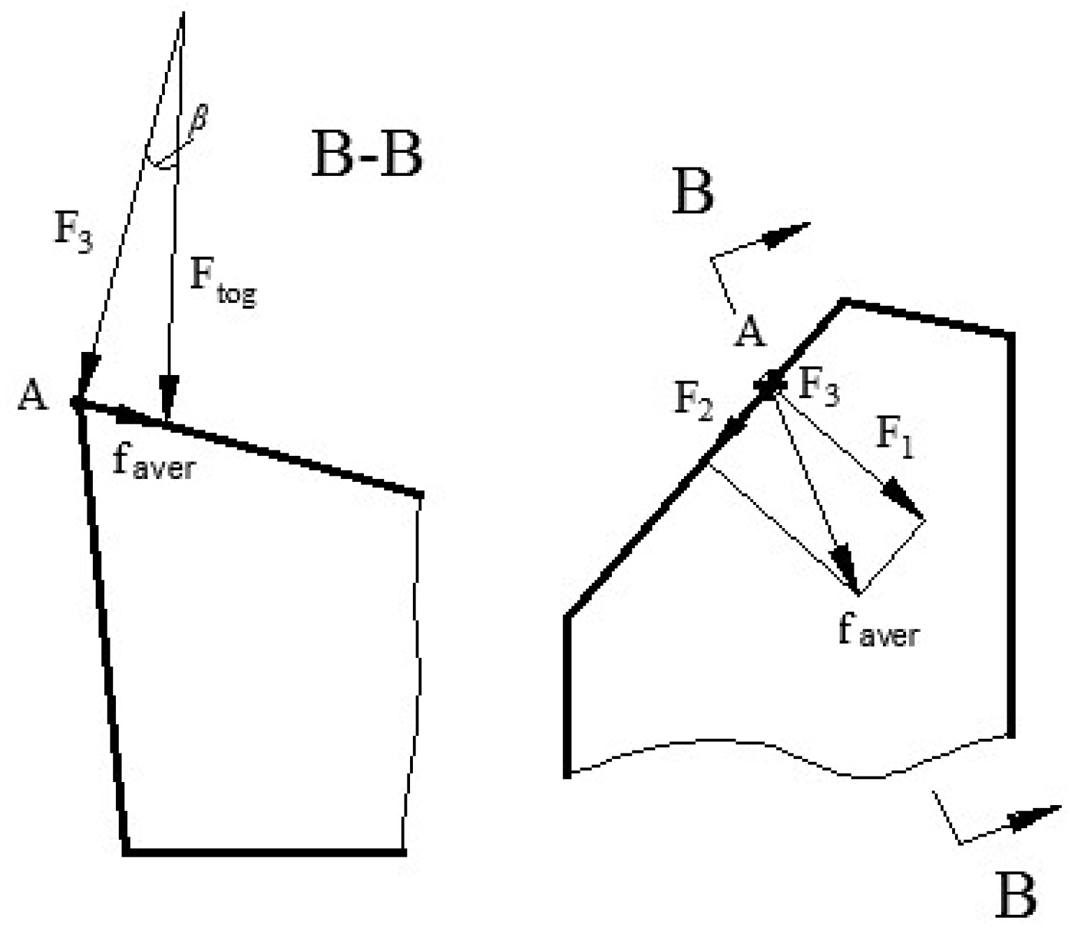
In this paper, the friction coefficient and friction angle are calculated using the equivalent force model and the turning experimental from turning, utilizing Formula (2). Friction angles are shown in Figure 4.
where F1 represents the cutting force perpendicular to the main cutting edge on the rake face, F2 represents the cutting force along the main cutting edge on the rake face, Faver represents the average friction force, F3 represents the cutting force perpendicular to the rake face, and β is the average friction angle.
4. Orthogonal Cutting Model
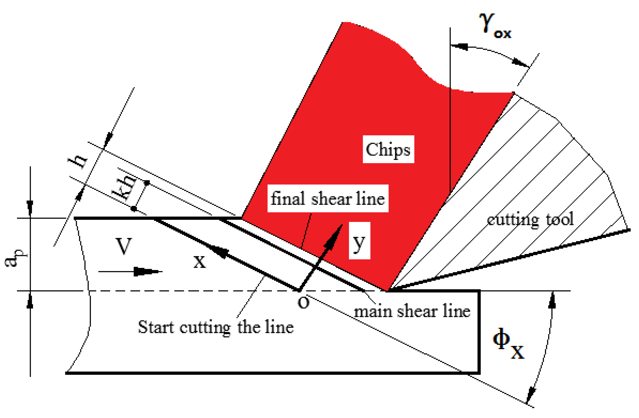
In this paper, we establish the milling force model of the straight groove milling cutter using it as an example. The main cutting edge of the straight slotted cutter is located discretely along the direction of the tool axis, which can be considered as an orthogonal cutting force model. Therefore, the orthogonal cutting force model can be used to calculate the shear stress of any micro-segment when modeling the milling force. The orthogonal cutting force model is established using the following three control equations. The modeling process is as follows [2]: First, the shear strain and shear strain rate in the shear zone are calculated using the deformation control equation. Then, the shear stress in the material control equation is substituted into the temperature control equation, resulting in the establishment of a first-order ordinary differential equation for temperature (T) with respect to the distance (y) from either the initial shear line to the primary shear line or from the primary shear line to the final shear line. The temperature distribution in the shear zone can be obtained through numerical integration. Finally, the shear stress and shear force on the main shear plane can be calculated by substituting the material control equation, allowing for the realization of the orthogonal cutting force modeling.
- (1)
- Deformation control equation
According to the variation in shear strain in the shear zone, the non-equal shear zone model [2] divides the shear zone into two unequal zones, as depicted in Figure 5. It is assumed that the distance from the main shear plane to the initial shear line is k times the thickness of the entire shear zone. Additionally, the shear strain rate reaches its maximum value on the principal shear plane. It is assumed that the shear strain rate follows a piecewise linear distribution within the shear zone. The shear strain rate and shear strain distribution of the non-equally divided shear zone model can be calculated using the following formula.
Since the shear strain distribution is the integral of the derivative of the shear strain, it can be obtained by integrating Equation (3) with respect to the derivative of the shear strain.
On the principal shear plane, the velocity in the shear direction is defined as zero.
Suppose that the shear angle in right-angle cutting satisfies Merchant’s formula.
where k is the coefficient of inequality, h is the thickness of the whole shear zone (taking h = 0.025 mm), q = 3 when the speed is low, Vx is the cutting speed at any point on the main cutting edge, is the shear strain rate, is the maximum shear strain rate, is the shear strain, is the friction angle of any section of the tool. The friction angle can be determined using the experimental value of the turning force, the equivalent front angle, the equivalent edge inclination angle and the equivalent principal declination angle obtained from the equivalent turning force model. The friction angle can be determined by applying Formulas (1)–(3). is the shear angle of any section of the tool, is the rake angle of any cutting tool section in the main section, and if the groove milling cutter is modeled, , is the radial rake angle of any section of the straight gear groove milling cutter. In the identification of the J–C material constitutive equation constant, is the rake angle of the turning tool in the main section.
- (2)
- Temperature control equation
Generally, when the cutting speed is high, heat conduction can be neglected, meaning that λ = 0. Therefore, the boundary of the shear band (from the initial shear line to the final shear line) can be considered as an adiabatic condition during the cutting process. Assuming that the fraction of plastic deformation work converted to heat is μ, the two-dimensional heat conduction equation in the steady-state flow condition can be simplified as follows:
where ρ represents the density of the material, and μ denotes the Taylor–Quinney coefficient. In this context, μ is assigned a value of 0.85 based on the relationship established by Rosakis et al. [25] between the Taylor–Quinney coefficient and plastic strain and the plastic strain rate.
The thermal boundary condition states that the temperature of the chip at the initial shear line is equal to the initial workpiece temperature, TW. Additionally, the initial workpiece temperature is approximately equal to the indoor temperature.
- (3)
- Material control equation
Considering the factors of work hardening and thermal softening that affect the flow stress of material, the Johnson–Cook constitutive equation is used in this paper. The expression is as follows:
where A represents the yield strength, B represents the hardening modulus, C represents the strain rate sensitivity coefficient, n represents the hardening index, m represents the heat softening index, γ represents the shear strain, represents the reference shear strain rate, represents the shear strain rate, T represents the instantaneous absolute temperature of the workpiece, Tr represents the initial workpiece temperature or room temperature, and Tm represents the melting temperature of the workpiece material.
It is necessary to know the flow stress parameters A, B, C, n and m in the constitutive equation of J–C material when calculating the shear stress of each micro-segment of the wheel-groove milling cutter using the orthogonal cutting force model. In this paper, the equivalent turning force model is utilized to enhance the precision of the rake angle and friction angle in the orthogonal cutting force model. The optimal flow stress parameters are obtained through the inverse identification method [8], using the data from the turning experiment and the parameters of the J–C material constitutive equation.
5. Johnson–Cook Inverse Identification of Constitutive Equation Parameters
According to the average friction angle and the equivalent front angle obtained from the turning experiment, as well as the equivalent turning force model, this paper calculates the experimental value of the flow stress. Subsequently, the theoretical flow stress value is calculated using the orthogonal cutting force model. Finally, the objective function is to minimize the error between the theoretical and experimental values, based on the initial constitutive parameters obtained from the split Thomas Hopkinson pressure bar (SHPB) experiment. The optimal values of the flow stress parameters A, B, C, n and m of the Johnson–Cook constitutive equation are obtained through the global searching capability of a genetic algorithm. The process of parameter identification is as follows:
- (1)
- The average friction force (Equation (2)) is calculated from the three-dimensional cutting force obtained from the turning experiment. The experimental value of flow stress is calculated using Formula (8).
- (2)
- Calculation of Theoretical Flow Stress
The equivalent rake angle is determined using the equivalent turning force model, which takes into account the impact of the rounded cutting edge radius, the tip arc and the feed speed on the tool’s geometric angle. The shear stress and theoretical flow stress on the main shear plane can be calculated by incorporating the shear stress and theoretical flow stress on the main shear plane it into the orthogonal cutting force model of Equations (3)–(6). The rake angle γox refers to the rake angle γo of the turning tool in the main section. It is used to calculate the shear stress and theoretical flow stress on the main shear plane.
- (3)
- The initial constitutive parameters were obtained from the split Hopkinson pressure bar (SHPB) test. The mean relative error between the theoretical flow stress σAB and the experimental flow stress σexp was utilized as the fitness function of the genetic algorithm, as depicted in Formula (9).
The optimal values of the Johnson–Cook constitutive equation parameters A, B, C, n and m are obtained using a genetic algorithm.
The initial population is generated randomly within the specified parameter range. Then, the individual is evaluated using the fitness function (Formula (9)), which calculates the probability of individual selection based on a smaller cumulative error. The individuals with a higher probability are more likely to pass on their characteristics to the next generation. The next generation is produced through individual selection, chromosome crossing and mutation. After a certain number of iterations, the fitness will steadily and the iteration will end.
The constitutive parameters of AISI 1045 steel have the following properties:
A = 507 MPa, B = 320 MPa, C = 0.064, n = 0.28 and m = 1.06.
The constitutive parameters of alloyed steel 34CrNi3Mo have the following properties:
A = 648 MPa, B = 459 MPa, C = 0.007, n = 0.12 and m = 1.36.
6. Groove Milling Cutter Milling Force Model
- (1)
- The geometric parameters of the groove milling cutter are shown in Figure 6.
The primary cutting edge of the groove milling cutter is axially distributed in the orthogonal cutting mode, and the axial dispersion of the cutter is equal to K.
And 0 ≤ x ≤ ap. The relationship between the radius Rx (Rx = dx/2) and the axial direction x at any section of the groove milling cutter can be determined using Figure 6, as shown below:
- (2)
- The cutting speed at any point on the main cutting edge is calculated using Formula (11).
- (3)
- Radial forward angle γrx
The radial rake angle γrx at any point on the main cutting edge of the straight-groove milling cutter, which is the angle between the inner base surface of the end section and the rake face, varies with the diameter of the grooved wheel core, as illustrated in Figure 7. Since the eccentricity (e) of the straight groove milling cutter is a constant, the eccentricity of the experimental groove milling cutter is 1.05. Pr is the base plane. The radial rake angle at any point of the groove milling cutter can be calculated using Formula (12). A is the basis for processing in Figure 7. The marks on the left of Figure 7 indicate that the circle bounces here by 0.01mm relative to reference A. The mark on the right of Figure 7 indicates that the cylindricity of the second half of the cylinder is 0.005mm.
where dx represents the diameter of the wheel core at any end section, and γrx denotes the radial rake angle of each micro-segment.
Assuming that the shear stress in the main shear plane is uniformly distributed, and the shear force is proportional to the shear strain. We can conclude that:
where Spraveri, j is the average cross-sectional area of the cutting layer in the base plane of the j-th microsegment of the i-th tool tooth, aaver is the average cutting thickness of the microsegment from cut-in to cut-out, and db is the cutting width of the microelement. The value of db can be determined by the extent of back cutting and the discrete number of cutting tools, K.
According to the force balance on the chip, the normal force perpendicular to the main shear plane can be determined.
where Fni,j represents the normal force acting perpendicular to the rake face of the milling cutter on the j-th microsegment of the i-th cutter tooth, β denotes the average friction angle, represents the shear angle of any cutter section, and γrx represents the radial rake angle of any given section.
- (1)
- The unit cutting force vector F0i,j is calculated as shown in Equation (15).
- (2)
- The cross-sectional area of the instantaneous cutting layer on the rake face (Sqi,j)
By calculating the unit cutting force vector on the rake face, it is possible to determine the instantaneous bending moment, torque and axial force. The calculation process is as follows:
- (1)
- The vector representing the cutting force vector of the micro-segment in three dimensions on the rake face of the micro-segment.
- (2)
- The cutting forces in the radial, tangential and axial directions (Fijr1, Fijt1 and Fija1)
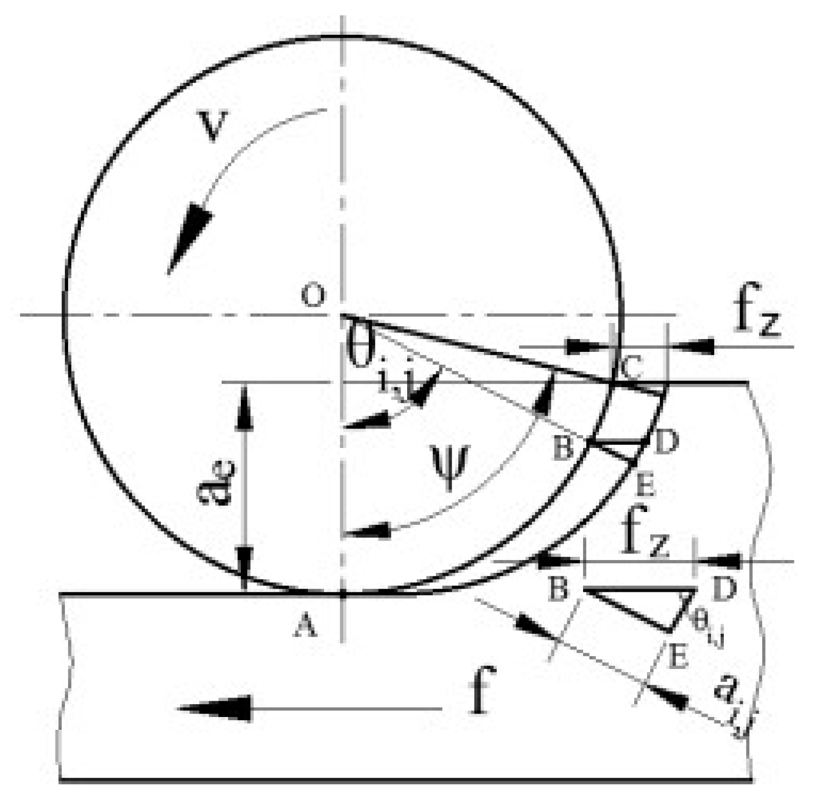
The transformation from the (r-t-a) coordinate system to the (r1-t1-a1) coordinates is achieved by rotating the angle around the axis of Fa, as shown in Figure 9. n is the speed of the wheel slot milling cutter in Figure 9.
By using Equation (19), the bending moment dMi,j and torque dMni,j of each segment can be calculated.
where lij represents the distance from the j-th cutting micro-segment of the i-th tooth to the end of the spindle of the machine tool.
- (3)
- Milling groove involves milling cutter turning moment, turning torque and axial resultant force.
The flowchart programmed using MATLAB software is shown in Figure 10.
First, the groove milling cutter is axially divided into sections, and the cutter is divided into equal parts along the axial direction. During the process of tool rotation, the increment of the tool rotation angle is ∆θ = ω × t, where w is the angular velocity, and the total number of rotations is L. Then, L = T/t (T is the period).
Secondly, the contact condition between each micro-segment of the tool and the workpiece is established.
where ψi,j represents the contact angle of each micro-segment, and ae denotes the cutting capacity of the side of the groove milling cutter.
According to the contact condition, it can be determined whether the tool is in contact with the workpiece. If there is contact, θi,j represents the turning angle of the cutter. If not, θi,j equals zero. Thus, the instantaneous cross-sectional area of each micro-segment of the cutting layer can be calculated. The three-dimensional cutting force on the rake face is then calculated using the unit cutting force vector. The tangential force, radial force and axial force are obtained through coordinate transformation. Finally, the bending moment, torque and axial direction of each micro-segment are calculated to predict milling forces for the groove milling cutter.
7. Equivalent Rake Angle Acquisition Method Based on Cutting Experiment
- (1)
- Equivalent Front Angle Acquisition Method Based on Turning Experiment
The equivalent turning force model is established through a turning experiment, which provides accurate values for the equivalent front angle. These values are used to identify constitutive equation of the J–C material.
In this study, a methodology based on pattern recognition technology has been developed to predict the Mean Reciprocal Rank (MRR). The spark field generated in most dry grinding processes is used to establish a model for predicting the MRR. A series of experiments are conducted to obtain the sample data. The area, density and energy spectrum characteristics of the spark field are extracted and quantified to serve as input for the training model. The least squares method and Support Vector Regression (SVR) are used to construct a continuous function with the spark field features as the input and the material removal rate as the output. The following conclusions can be drawn.
(1) Turning experimental device system, as shown in Figure 11:cutting experiments were conducted on the CK6132 lathe using the Swiss KISTLER9257B dynamometer, Kistler5070A charge amplifier, DEWE3020 digital acquisition system and Industrial Control Computer. CK6132 is a machine tool manufactured by Shenyang Machine Tool (Group) Co., Ltd. in Shenyang, China. The experimental device system is shown in Figure 11. The system integrates a 16-channel ADC card and data analysis software Dewesoft-6-se. Coolant is used during the cutting process.
(2) Specimen: The material is alloyed steel 34CrNi3Mo. The diameter of the specimen is Φ150 mm, and its length is 450 mm in order to ensure the rigidity of the technological system.
(3) Tooling and alignment: One end is used to hold the workpiece with a chuck jaw, while the other end is supported by a center. The alignment using the dial meter helps ensure that the rotating center and three-jaw Chuck has a coaxial error of Δ ≤ 0.02.
(4) Cutting tool: The material the cutting tool is made out of is ZY12UF, which complies with ISO International Standard K30. The cross-sectional dimensions of the cutting tool are B = 20 mm and H = 20 mm. The geometric parameters of cutting tool and cutting tool are provided by Chengdu Tool Research Institute Co., Ltd., and these parameters are shown in Table 1.
(5) Setting of cutting parameters
When using a 45° cylindrical turning tool to turn a workpiece, the cutting edge of the tool is positioned higher than the center of the workpiece, with a height (h) of 0.4 mm. The angle of the tool installation is 0.46 degrees. The cutting speed is V = 80 ~ 100 m/min.
The nominal cross-sectional area S was set at 0.2 mm2, 0.25 mm2, 0.3 mm2, 0.35 mm2 and 0.4 mm2 in the base plane, where S = ap × f.
The back-eating capacity ap = 1.1 mm, 1.2 mm, 1.3 mm, 1.4 mm and 1.5 mm. The corresponding feed values f were calculated using S and ap.
- (2)
- Equivalent angle analysis
(1) The absolute value of the rake angle increases with the increase in the cross-sectional area of the cutting layer, but the increase is minimal. The influence of the arc radius of the tool tip on cutting force and chip flow direction can be minimized by increasing the amount of back cutting tool [9].
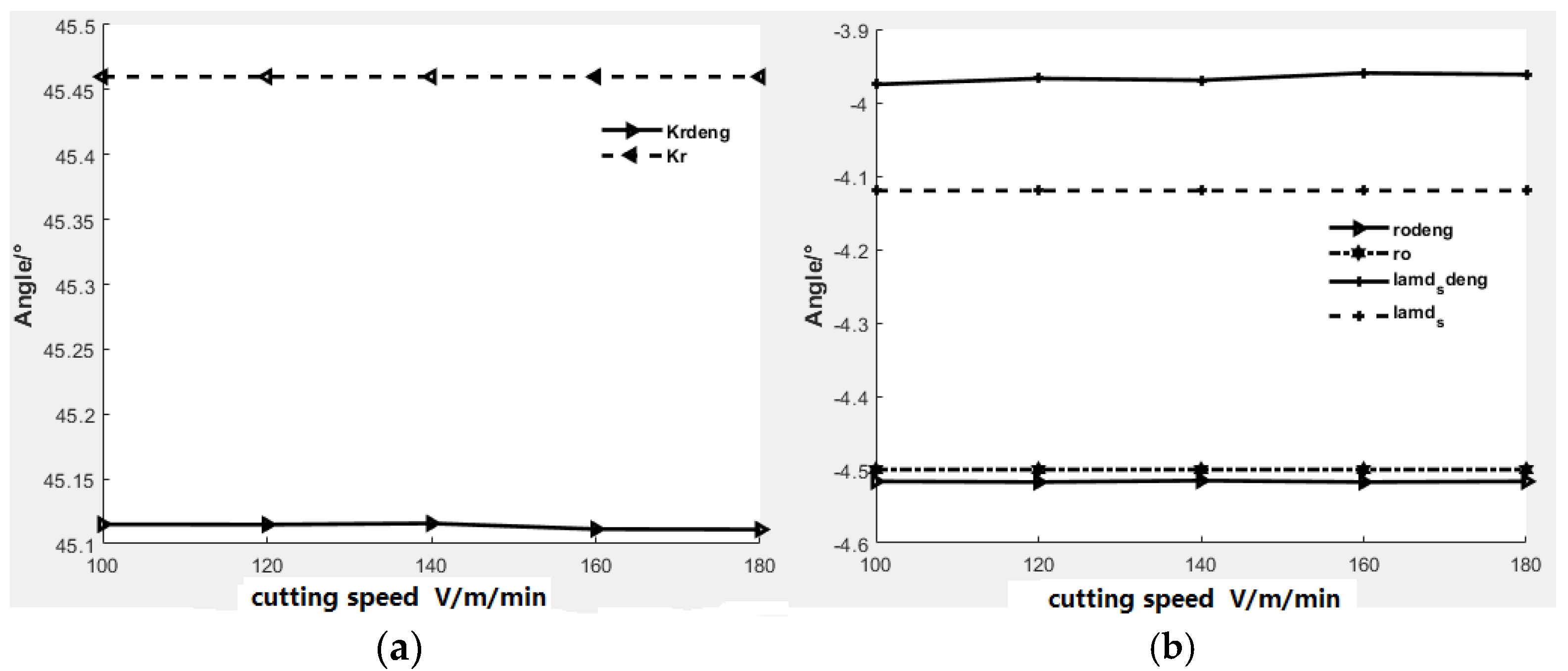
(2) The variation in the equivalent principal declination angle (Kreequ), equivalent edge inclination angle (λseequ) and equivalent rake angle (γoeequ) with cutting speed.
As depicted in Figure 12, the equivalent principal deflection angle, the equivalent rake angle and the equivalent edge inclination angle tend to remain constant when the cutting speed is changed. This means that the cutting speed does not affect the equivalent post-geometry angles of the tool. Therefore, the equivalent rake angle remains constant when using the slot milling cutter to cut the workpiece at different cutting speeds.
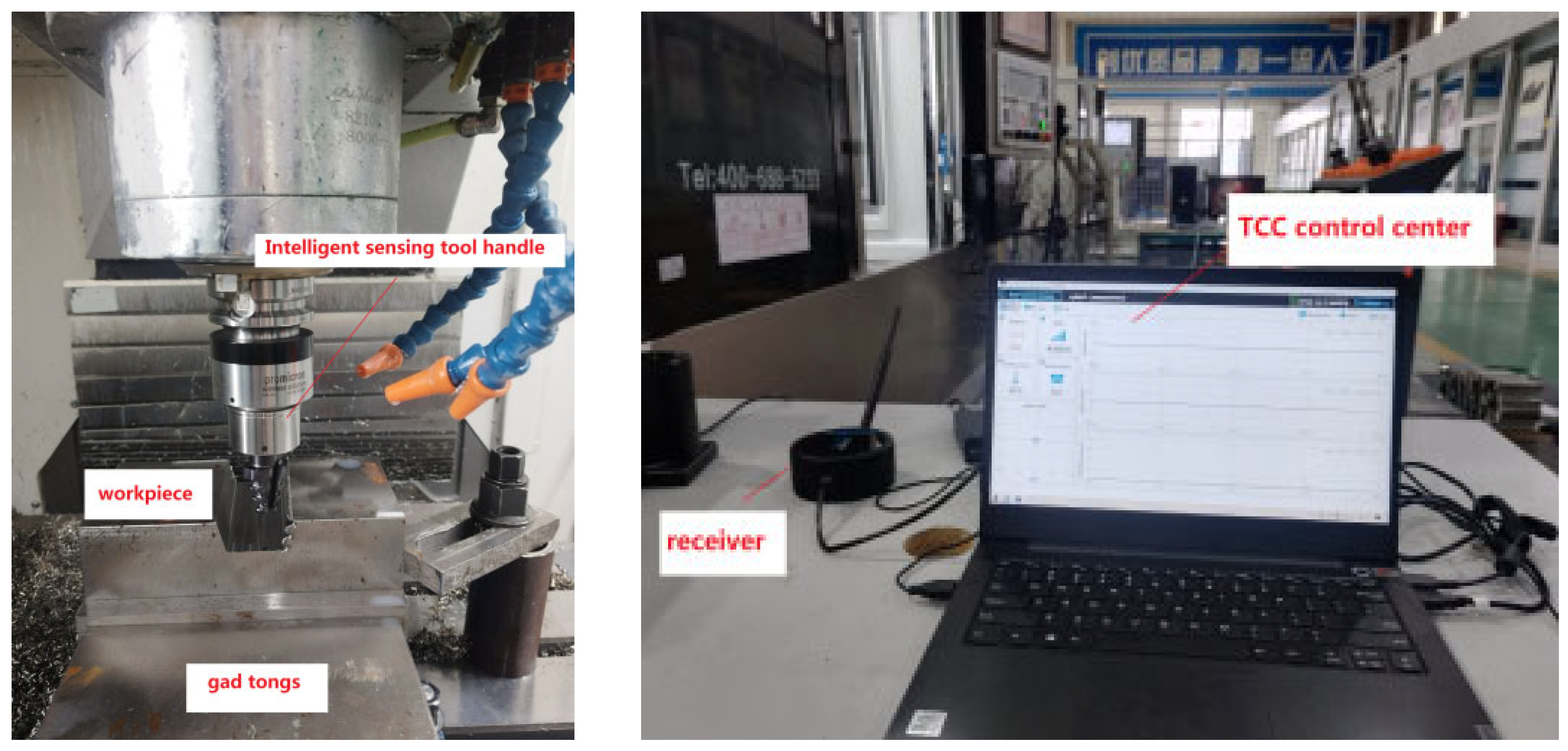
8. Verification of Milling Force Prediction Model of Groove Milling Cutter
The experimental milling device system is shown in Figure 13. Milling 34CrNi3Mo on the EV850L machining center during wet cutting experiments. The intelligent induction handle used is BT40_MAGE20_NL105, and data acquisition is READ1.2. In this paper, the milling force of single-side inverse milling of a workpiece with a straight groove milling cutter is measured using the Spike wireless milling force measuring system.
- (1)
- The material of the groove milling cutter is ZY12UF, and it conforms to the ISO International Standard K30.
- (2)
- The experimental process of groove milling is as follows:
- Groove milling with Φ12 mm end mills of.
- The bevel groove is machined using a taper milling cutter, and the taper matches that of the wheel groove milling cutter.
- The groove milling cutter utilizes reverse milling on one side of the workpiece to cut the full tooth.
- The milling experiment was carried out with a groove milling cutter.
The cutting parameters for AISI 1045 steel and alloyed steel 34CrNi3Mo are as follows: V = 80 m/min, feed rate per tooth fz = 0.015 mm/z, ap = 20 mm and ae = 0.2 mm.
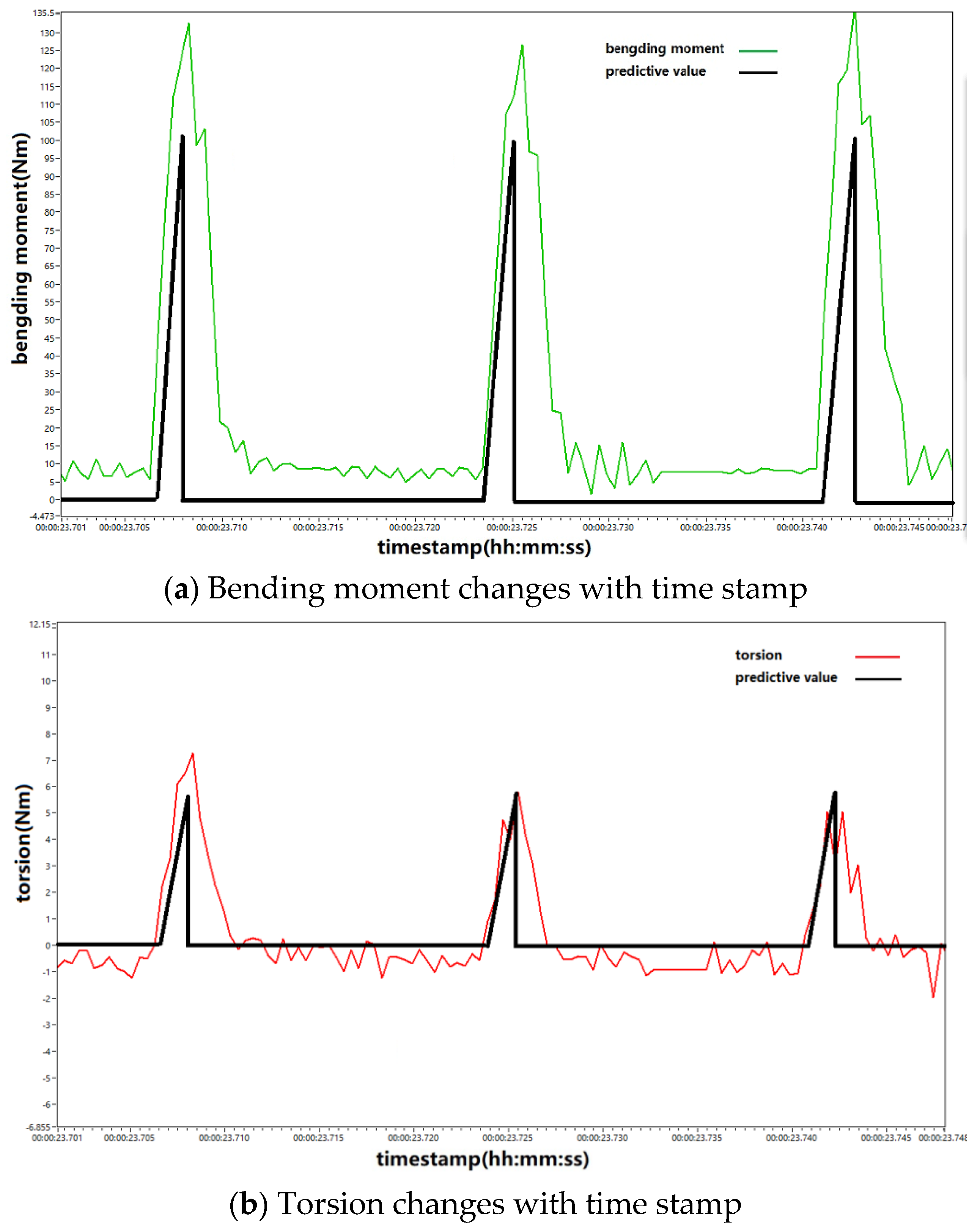
Figure 14 shows a comparison between the experimental and predicted values of bending moment, torsion and tension/pressure during the cutting of alloyed steel 34CrNi3Mo over time.
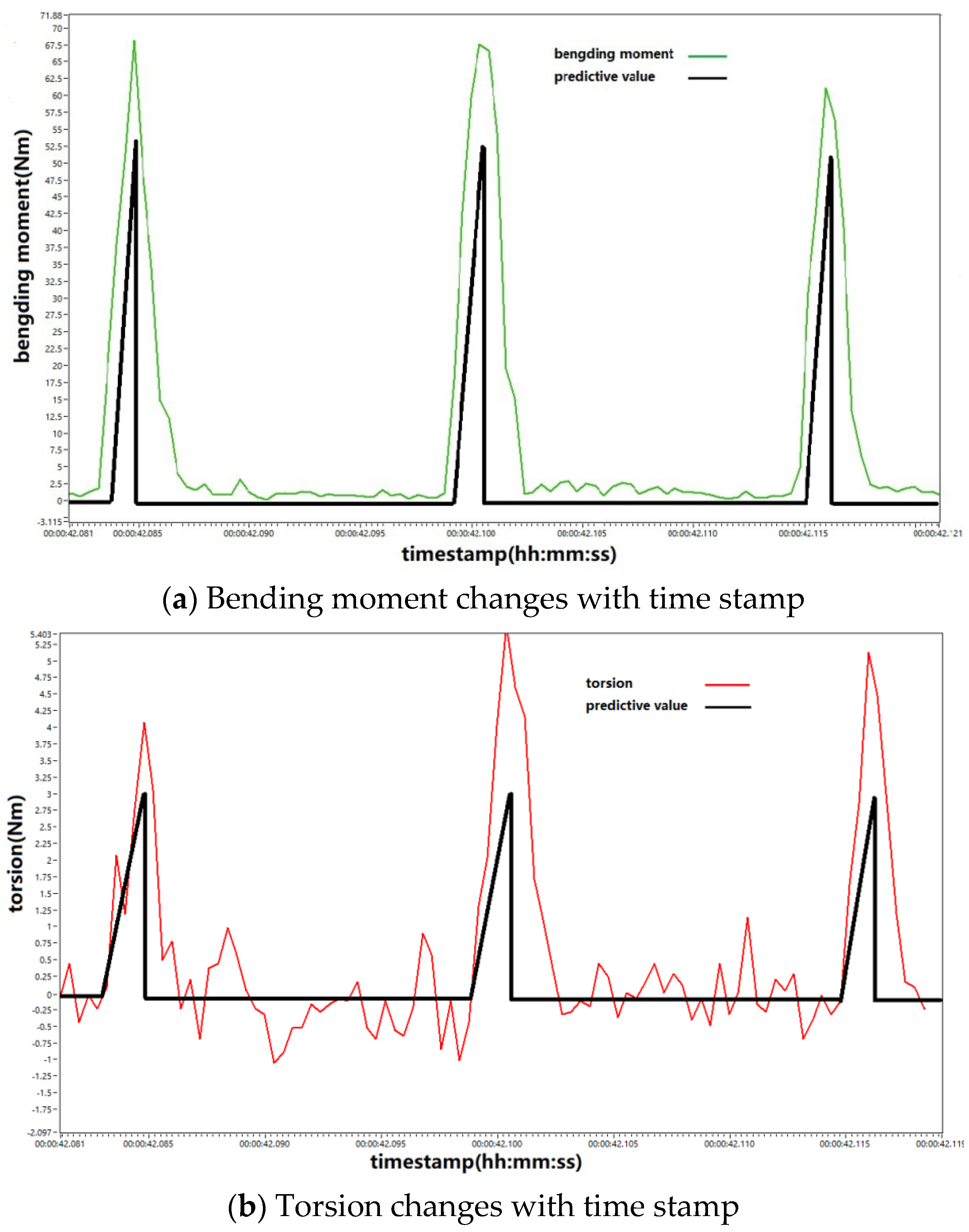
Figure 15 shows the comparison of experimental and predicted values of bending moment, torsion and tension/pressure when cutting AISI 1045 steel.
It can be seen from Figure 14 and Figure 15 that the three wave peaks predicted by the theory of bending moment and torque are almost the same size. However, due to the anisotropy of the material, the axial runout and rotation accuracy of the machine tool spindle, the predicted values show good agreement with the experimental values in terms of bending moment and torque. The main reasons for the error are as follows: (1) The assumption that the cutter is a rigid body is incorrect. In actual production, the cutter experiences elastic deformation, leading to vibration. These vibrations can be accurately determined by analyzing the experimental values of the axial force. (2) The plough force produced by the contact between the flank and the workpiece is not considered. The effect of the third deformation zone on the cutting force is not considered.
9. Conclusions
Based on the prediction model of equivalent turning force and the unequal orthogonal cutting force model, this paper establishes the milling force model for a groove milling cutter.
(1) The effective turning force model, which synthetically considers factors such as the arc radius of the tool tip, the arc radius of the cutting edge and the working angle, provides accurate rake angles and average friction angles at different cutting speeds for the identification method of the J–C material constitutive equation. The optimal values of the flow stress parameters in the J–C material constitutive equation were obtained using the orthogonal cutting force model and the genetic algorithm.
(2) Firstly, the straight groove milling cutter is discretized based on the obtained optimal material constitutive parameters. Secondly, the micro-segments calculate the shear force according to the three control equations in the orthogonal cutting force model. Then, the bending moment, torque and axial force of the wheel-groove milling cutter are calculated using coordinate transformation. Finally, the prediction model for the milling force of the wheel-groove milling cutter has been established, and the validity of the model has been verified through experiments. This ensures that the model can accurately predict the changing trend and magnitude of the instantaneous milling force when working with different materials and cutting speeds. This method provides the mechanical basis for enhancing the tool life and improving the profile quality.
Author Contributions
Conceptualization, M.W.; methodology, M.W. and T.W.; validation, M.W.; formal analysis, M.W. and R.W.; data curation, M.W. and T.W.; investigation, M.W.; supervision, G.Z.; project administration, G.Z.; funding acquisition, G.Z.; writing—original draft preparation, T.W. and R.W.; writing—review and editing, M.W., T.W. and R.W.; visualization, M.W. and T.W. All authors have read and agreed to the published version of the manuscript.
Funding
This work was supported by the National Natural Science Foundation of China (grant number 5227053643), the Shaanxi Natural Science Foundation Project (grant number 2023-JC-QN-0428) and 2022 Provincial Science and Technology Plan Special Factor Method Transfer Payment Project (grant number MZGXQ2023KJ004).
Institutional Review Board Statement
Not applicable.
Informed Consent Statement
Not applicable.
Data Availability Statement
The datasets used or analyzed during the current study are available from the corresponding author on reasonable request.
Conflicts of Interest
The authors declare no conflict of interest.
References
- Oxley, P.L.B. Mechanics of Machining; Ellis Horwood: Chichester, UK, 1989. [Google Scholar]
- Li, B.-L.; Wang, H.-L.; Hu, X.-J.; Li, C.-G. Thermomechanical Modeling and Simulation Analysis of Oblique Cutting. China Mech. Eng. 2010, 21, 2402–2408. [Google Scholar]
- Merchant, M.E. Mechanics of the Metal Cutting Process, Orthogonal Cutting. J. Appl. Phys. 1945, 16, 318–324. [Google Scholar] [CrossRef]
- Lee, E.H.; Shaffer, B.W. The Theory of Plasticity Applied to a Problem Machining. J. Appl. Mech. 1951, 18, 405–413. [Google Scholar] [CrossRef]
- Morcos, W.A. A Slip Line Field Solution of the Free Continuous Cutting Problem in Conditions of Light Friction at Chip-tool Interface. J. Eng. Ind. 1980, 102, 310–314. [Google Scholar] [CrossRef]
- Shamoto, E.; Altintas, Y. Prediction of Shear Angle in Cutting with Maximum Shear Stress and Minimum Energy Principles. J. Manuf. Sci. Technol. 1999, 121, 399–407. [Google Scholar] [CrossRef]
- Pang, L.; Kishawy, H.A. Modified Primary Shear Zone Analysis for Identification of Material Mechanical Behavior during Machining Process Using Genetic Algorithm. Manuf. Sci. Eng. 2012, 134, 041003. [Google Scholar] [CrossRef]
- Pan, P.F.; Song, H.W.; Ren, G.Q.; Yang, Z.H.; Xiao, J.F.; Chen, X.; Xu, J.F. Reverse Identification of High-Temperature Constitutive Parameters of Fused Silica Based on Orthogonal Cutting Theory. Sci. Sin. Technol. 2020, 50, 1426–1436. [Google Scholar]
- Yucesan, G.; Altintas, Y. Improved Modelling of Cutting Force Coefficients in Peripheral Milling. Int. J. Mach. Tools Manuf. 1994, 34, 473–487. [Google Scholar] [CrossRef]
- Budak, E.; Altintas, Y.; Armarego, E.J.A. Prediction of Milling Force Coefficient from Orthogonal Cutting Data. J. Manuf. Sci. Eng. 1996, 118, 216–224. [Google Scholar] [CrossRef]
- Lee, P.; Altinas, Y. Prediction of Ball-End Milling Forces from Orthogonal Cutting Data. Int. J. Mach. Tools Manuf. 1996, 36, 1059–1072. [Google Scholar] [CrossRef]
- Altintas, Y.; Lee, P. Mechanics and Dynamics of Ball End Milling. J. Manuf. Sci. Eng. 1998, 120, 684–692. [Google Scholar] [CrossRef]
- Engin, S.; Altinas, Y. Mechanics and Dynamics of General Milling Cutters. Part I: Helical End Mills. Int. J. Mach. Tools Manuf. 2001, 41, 2195–2212. [Google Scholar] [CrossRef]
- Yun, W.S.; Cho, D.W. Accurate 3-D Cutting Force Prediction Using Cutting Condition Independent Coefficients in End Milling. Int. J. Mach. Tools Manuf. 2001, 41, 463–478. [Google Scholar] [CrossRef]
- Yoon, M.C.; Kim, Y.G. Cutting Dynamic Force Modeling of End Milling Operation. J. Mater. Process. Technol. 2004, 155, 1383–1389. [Google Scholar] [CrossRef]
- Omar, O.E.E.K.; EI-Wardany, T.I.; Ng, E.; Elbestawi, M. An Improved Cutting Force and Surface Topography Prediction Model in End Milling. J. Mater. Process. Technol. 2009, 209, 2532–2544. [Google Scholar] [CrossRef]
- Wan, M.; Zhang, W.H. Investigation on Cutting Force Modeling and Numerical Prediction of Surface Errors in Peripheral Milling of Thin-Walled Workpiece. Acta Aeronaut. Astronaut. Sin. 2005, 5, 598–603. [Google Scholar]
- Cheng, Q.L.; Ke, Y.L.; Dong, H.Y. Numerical Simulation Study on Milling Force for Aerospace Aluminum Alloy. Acta Aeronaut. Astronaut. Sin. 2006, 4, 724–727. [Google Scholar]
- Xu, L.; Schueller, J.K.; Tlusty, J. A Simplified Solution for the Depth of Cut in Multi-Path Ball End Milling. Mach. Sci. Technol. 1998, 2, 57–75. [Google Scholar] [CrossRef]
- Kim, G.M.; Cho, P.J.; Chu, C.N. Cutting Force Prediction of Sculptured Surface Ball-End Milling Using Z-Map. Int. J. Mach. Tools Manuf. 2000, 40, 277–291. [Google Scholar] [CrossRef]
- Lazoglu, I. Sculpture Surface Machining: A Generalized Model of Ball-End Mill Force System. Int. J. Mach. Tools Manuf. 2003, 43, 453–462. [Google Scholar] [CrossRef]
- Lamikiz, A.; López de Lacalle, L.N.; Sanchez, J.A.; Salgado, M.A. Cutting Force Estimation in Sculptured Surface Milling. Int. J. Mach. Tools Manuf. 2004, 44, 1511–1526. [Google Scholar] [CrossRef]
- Becze, C.E.; Elbestawi, M. A Chip Formation Based Analytic Force Model for Oblique Cutting. Int. J. Mach. Tools Manuf. 2002, 42, 529–538. [Google Scholar] [CrossRef]
- Wu, M.Z.; Zhang, G.P.; Gou, J.F.; Zhang, P. Research on Modeling Method of Equivalent Turning Force Model. J. Mech. Strength 2023, 45, 715–722. [Google Scholar]
- Rosakis, P.; Rosakis, A.J.; Ravichandran, G.; Hodowany, J. A Thermodynamic Internal Variable Model for the Partition of Plastic Work into Heat and Stored Energy in Metals. J. Mech. Phys. Solids 2000, 48, 581–607. [Google Scholar] [CrossRef]
Figure 1.
General idea map to calculate the milling force model.

Figure 2.
Schematic diagram of equivalent method for indexable turning tools.

Figure 3.
Schematic diagram of coordinate transformation applied in the turning tool.

Figure 4.
Friction angle calibration method.

Figure 5.
A sketch of the unequal shear region.

Figure 6.
Geometric parameters of straight groove milling cutter.

Figure 7.
Radial rake angle of slot milling cutter.

Figure 8.
Cutting thickness in the milling operation.

Figure 9.
Coordinate transformation applied in the groove milling cutter.

Figure 10.
Flow chart of milling force prediction for groove milling cutter.

Figure 11.
Setup of the turning device for experimental data acquisition.

Figure 12.
Variation of tool equivalent geometric angle with cutting speed. (a) Variation of equivalent principal declination angle with cutting speed. (b) Variation of equivalent rake angle and edge inclination angle with cutting speed.
Figure 12.
Variation of tool equivalent geometric angle with cutting speed. (a) Variation of equivalent principal declination angle with cutting speed. (b) Variation of equivalent rake angle and edge inclination angle with cutting speed.

Figure 13.
Apparatus of milling experiment.

Figure 14.
Comparison of experimental and predicted values of bending moment (a), torsion(b) and tension/pressure(c) in cutting alloyed steel 34CrNi3Mo.
Figure 14.
Comparison of experimental and predicted values of bending moment (a), torsion(b) and tension/pressure(c) in cutting alloyed steel 34CrNi3Mo.


Figure 15.
Comparison of experimental and predicted values of bending moment (a), torsion (b) and tension/pressure(c) when cutting AISI 1045 steel.
Figure 15.
Comparison of experimental and predicted values of bending moment (a), torsion (b) and tension/pressure(c) when cutting AISI 1045 steel.


Table 1.
Geometric parameters and coating of 45° turning tools.
| Geometric Parameters and Coating of Turning Tool | Symbols | Size | Unit |
|---|---|---|---|
| Anterior Horn | γo | −4.5 | degree |
| Back Angle | αo | 19.8 | degree |
| Edge inclination | λs | −4.12 | degree |
| Edge radius | 0.03 | mm | |
| Arc Radius of tool tip | r | 0.8 | mm |
| Principal Deflection Angle Kr | Kr | 45 | degree |
Disclaimer/Publisher’s Note: The statements, opinions and data contained in all publications are solely those of the individual author(s) and contributor(s) and not of MDPI and/or the editor(s). MDPI and/or the editor(s) disclaim responsibility for any injury to people or property resulting from any ideas, methods, instructions or products referred to in the content. |
© 2023 by the authors. Licensee MDPI, Basel, Switzerland. This article is an open access article distributed under the terms and conditions of the Creative Commons Attribution (CC BY) license (https://creativecommons.org/licenses/by/4.0/).
Share and Cite
MDPI and ACS Style
Wu, M.; Zhang, G.; Wang, T.; Wang, R. Milling Force Modeling Methods for Slot Milling Cutters. Machines 2023, 11, 922. https://0-doi-org.brum.beds.ac.uk/10.3390/machines11100922
AMA Style
Wu M, Zhang G, Wang T, Wang R. Milling Force Modeling Methods for Slot Milling Cutters. Machines. 2023; 11(10):922. https://0-doi-org.brum.beds.ac.uk/10.3390/machines11100922
Chicago/Turabian StyleWu, Mingzhou, Guangpeng Zhang, Tianle Wang, and Rui Wang. 2023. "Milling Force Modeling Methods for Slot Milling Cutters" Machines 11, no. 10: 922. https://0-doi-org.brum.beds.ac.uk/10.3390/machines11100922
Note that from the first issue of 2016, this journal uses article numbers instead of page numbers. See further details here.