Fluid–Structure Interaction Modeling Applied to Peristaltic Pump Flow Simulations

Abstract

In this study, fluid–structure interaction (FSI) modeling was applied for predicting the fluid flow in a specific peristaltic pump, composed of one metallic roller and a hyperelastic tube pumping a viscous Newtonian fluid. Hyperelastic material dynamics and turbulence flow dynamics were coupled in order to describe all the physics of the pump. The commercial finite element software ABAQUS 6.14 was used to investigate the performance of the pump with a 3D transient model. By using this model, it was possible to predict the von Mises stresses in the tube and flow fluctuations. The peristaltic pump generated high pressure and flow pulses due to the interaction between the roller and the tube. The squeezing and relaxing of the tube during the operative phase allowed the liquid to have a pulsatile behavior. Numerical simulation data results were compared with one cycle pressure measurement obtained from pump test loop data, and the maximum difference between real and simulated data was less than 5%. The applicability of FSI modeling for geometric optimization of pump housing was also discussed in order to prevent roller and hose parts pressure peaks. The model allowed to investigate the effect of pump design variations such as tube occlusion, tube diameter, and roller speed on the flow rate, flow fluctuations, and stress state in the tube.

1. Introduction

The peristaltic pump is a pumping device that is based on the peristalsis principle. The specific pump of this work was composed of a cylindrical rotor that squeezed and relaxed an elastic pipe where the fluid flows. In addition, during the operative phase, the pipe was submitted to high stress values, which might have caused such high deformation on the pipe that it affected the liquid’s transport. Experimental analysis could be used for developing pressure peak, pump optimizing, and for selecting optimal piping material. A feasible alternative to experimental analysis is the numerical simulation where important design variables could be systemically studied. From experimental sensitivity analysis, the Poisson’s coefficient of the tube material was very important. The Poisson coefficient (also called transversal contraction coefficient) is a property of each material, depending on the temperature, which measures the degree to which the material sample shrinks or dilates transversely in the presence of a longitudinal unidirectional stress.

The values of the Poisson’s coefficient for materials in nature are between 0 and 0.5; the value 0.5 corresponds to a virtually incompressible material (the rubber, for example, has values close to 0.5) which therefore has an infinite volumetric expansion module.

The peristaltic pump tubes are usually made of materials such as silicone, PVC, and other polymers that can offer, in addition to the aforementioned mechanical characteristics, also a remarkable chemical compatibility with solvents, acids, inks, paints, etc. Elastomers reinforced with textile inserts are used to guarantee the toughness of the pipe even at high pressures and for a long time.

The peristaltic pump is used in all processes in which the treated fluid has to get far from the pump components for safety reasons against contamination, such as in the food, pharmaceutical, and medical industries, or when products with solids in suspension must be dosed without being damaged. This type of pump allows to accurately calibrate the flow rate and keep it constant. These characteristics make it ideal where precision on the dosages and repeatability of the measurement are indispensable requirements such as in chemical laboratories, in bio-research, etc.

The need for a more accurate control of fluid flow for applications in Medicine and Engineering has increased the interest in performing numerical simulations. The control of the fluid flow derives from the fluid-induced deformation or the boundary moving induced deformation. The simple hose of the peristaltic pump’s structure can perform control and non-blocking high pressure, or even shock pressure, pumping throughout pipe deformations caused by the pump actuator parts. Furthermore, the high deformation may cause permanent damage for the hyperelastic pipe that affects liquid transport—optimal tubing material can be developed by pressure peak of the pumps.

The design of a peristaltic pump requires an accurate modelling [1,2]. The pump could be considered as a multibody model [3,4,5,6] and used in engineering applications [7,8,9] for dynamic simulations [10,11]. Active vibration control is another aspect to consider during the design phase [12]. Dynamic analysis [13] of each considered problem has some peculiar difficulties. In [14], the authors describe the influence of peristaltic fluid flow (blood) on the elastic boundaries (the blood vessel); in this case FSI problem is approached [15,16,17].

To describe an accurate model behavior of peristaltic pumps, fluid and solid models have to be merged—fluid flow is caused by pipe squeezing. The deformation of the tube is strongly coupled to the fluid flow, so an FSI analysis is required; then FSI modeling is mainly spread for pulsatile flow induced by moving domain. The data results are compared to the relative fixed boundary domain flow problems because of the small deformation of the domain, contrary to the hose system. Elabbasi [18] investigated the performance of a 180-degree rotary peristaltic pump with two metallic rollers by using 3D FSI with COMSOL Multiphysics. The model merges the fluid and structural parts in a monolithic way—the structure and the fluid parts are respectively described by Mooney-Rivlin hyperelastic material model and laminar flow models. However, the authors do not give any details on mathematics and they exclude any turbulence phenomena for the fluid. Zhou [19] described a 2D CFD tool for studying peristaltic pumps using ANSYS Fluent. This program code allowed to approach the Computational Mechanics [20,21,22], and it was also used to perform the control of nonlinear vibrations [23,24,25] for the machine design [26,27,28]. Further, it allowed the determination of the algorithms for computing the modal parameters of linear mechanical systems [29,30].

Therefore, this study aimed to develop a mathematical and numerical 3D transient FSI model for an industrial peristaltic pump. The main design variables governing pump performance were the pump speed, inner tube diameter, tube material, degree of tube occlusion, and back pressure. The model has been implemented in commercial software ABAQUS and catches the pipe deformation by a Neo-Hookean hyperelastic model and the fluid flow by the RNG κ–ϵ turbulence model. The mesh equation was described as a dynamic harmonic meshing function [31]. Therefore, through this study, it was seen that it is possible to simulate the operating conditions of a peristaltic pump and to obtain a numerical model of the peristaltic pump considered that allowed to perform a better study of the working phase aimed to improve and to optimize the operating characteristics of the peristaltic pump considered.

2. Geometry and Model

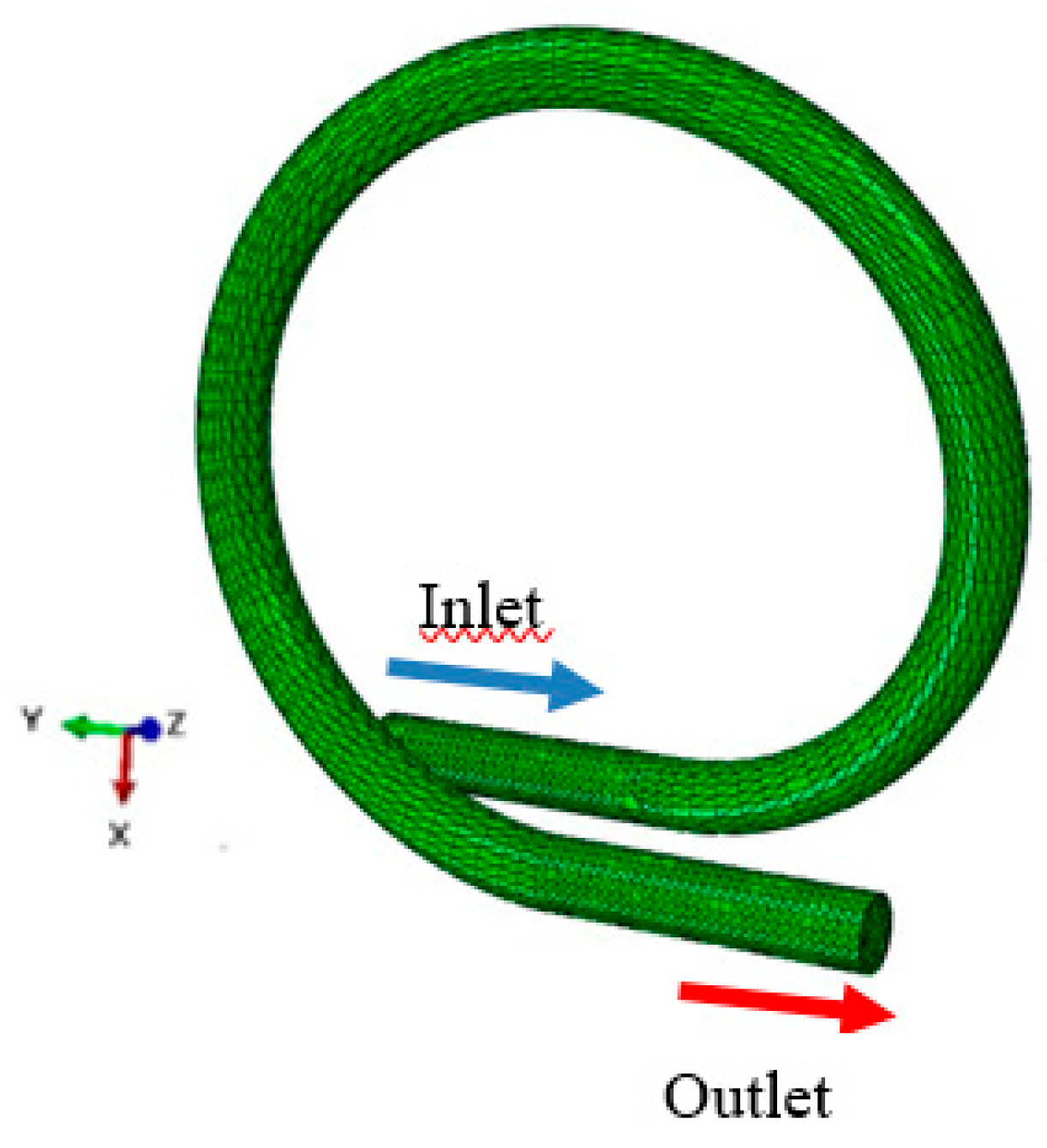
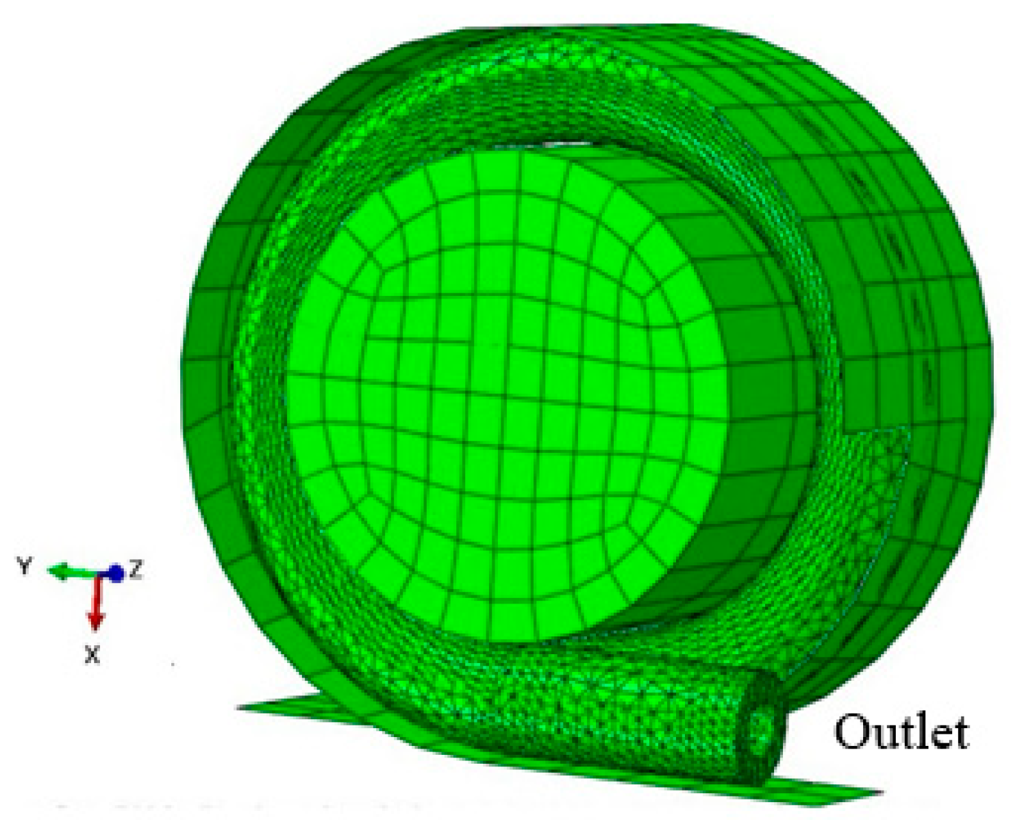
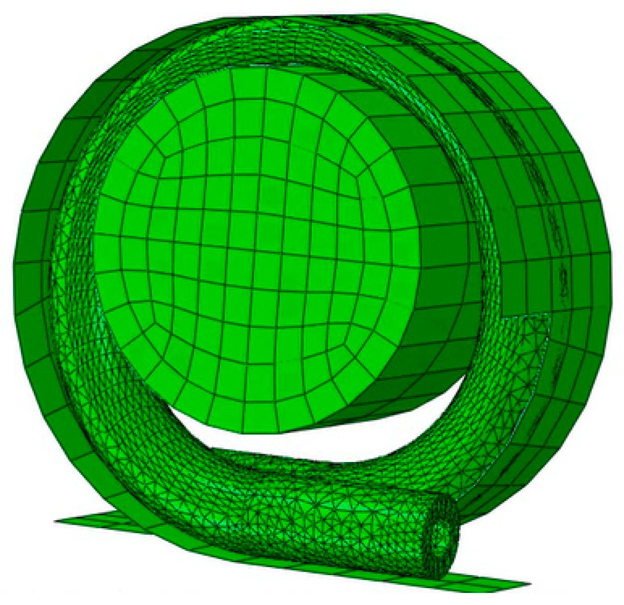
2.1. Model Geometry and Finite Element Mesh

In the peristaltic pump, a rotating roller squeezes a resilient pipe and the fluid is pushed forward through the hose pipe with compression and relaxation phases, see Figure 1. The rotation period of the roller and distance of roller axis from pipe axis affects the fluid flow along the hose pipe.

The FSI model of the peristaltic pump consisted of a cylindrical rigid roller, a round helix hose pipe, and a cylindrical rigid frame that covered the device and bounded the pipe movement during the squeezing phase. The features of the pipe made essential a 3D analysis of the phenomenon.

Radius of the rigid roller was 132.5 mm, and the pipe had a thickness of 15 mm, an internal radius of 32 mm, and an external one of 146 mm. The inertial property of the roller was neglected.

The structural part was meshed using 145 rectangular linear shell elements for the fixed frame, 40058 tetrahedral quadratic elements for the hose pipe ${\Omega }^s$, 208 hexahedral linear elements for the roller ${\Omega }^r,$ see Figure 2. The reference fluid domain, ${\Omega }_0^f$, was meshed using 46994 tetrahedral elements, as in Figure 3. The boundary layer had size 9% of the global mesh size and it consisted of 5 layers.

The height of the wall boundary layer during the squeezing was observed as having a significant effect on the velocity field convergence. The fluid and structure geometries were separately meshed but the element nodes on the common boundary coincided.

2.2. Mathematical Model

The finite deformations of the pipe in peristalsis phenomena rise up turbulent structures in a transient analysis. A turbulence model is needed to imitate actual flows in hose pumps and in order to model the fluid sub-problem. A RANS-based model is a compromise between the computational cost and the efficient of the results for FSI phenomena [32,33,34,35,36].

The fluid is described in an Arbitrary Lagrangian Eulerian framework. The ALE derivative induced by a deformation of fluid domain, $\varphi :{\Omega }_0^f\times I\to R^3$ for a scalar function $f:{\Omega }_0^f\times I\to R$ is defined as

$$\frac{D^{\varphi }f}{Dt}:=\frac{\partial f}{\partial t}+\frac{\partial \varphi }{\partial t}·\nabla f$$

(1)

The deformed fluid domain is defined as $\forall t\in I$ as ${\Omega }_t^f:=\varphi ({\Omega }_0^f,t).$ The fluid motion was described by the RNG κ–ϵ turbulence model in an ALE framework

$$\{\begin{array}{c}{\rho }^f\frac{D^{\varphi }{U}^f}{Dt}+{\rho }^f\left(U^f-w\right)\nabla U^f=-\nabla P^f+\left({\mu }^f+{\mu }_t\right)\Delta U^f-\frac{2}{3}\nabla k\\ \nabla ·U^f=0\\ {\rho }^f\frac{D^{\varphi }k}{Dt}+{\rho }^f\left(U^f-w\right)·\nabla k=\left({\mu }^f+\frac{{\mu }_t}{{\sigma }_k}\right)\Delta k-{\rho }^fϵ+P_k\\ {\rho }^f\frac{D^{\varphi }ϵ}{Dt}+{\rho }^f\left(U^f-w\right)·\nabla ϵ=\left({\mu }^f+\frac{{\mu }_t}{{\sigma }_{ϵ}}\right)\Delta ϵ-C_{2ϵ}{\rho }^f\frac{{ϵ}^2}{k}ϵ+\frac{ϵ}{k}{C}_{1ϵ}{P}_k-R_{ϵ}\end{array}$$

(2)

where $U^f$ is the mean velocity field, $P^f$ is the mean pressure, $k$ is the turbulent kinetic energy, $ϵ$ is the turbulent dissipation energy, ${\rho }^f$ is the fluid density, μ^f is the fluid dynamic viscosity, $P_k$ is the rate of production of turbulence, $R_{ϵ}$ is the rate of dissipation, and ${\mu }_t$ is the turbulent dynamic viscosity. The coefficient ${\sigma }_k$, ${\sigma }_{ϵ}$, $C_{1ϵ}$, and $C_{2ϵ}$ are closure coefficients. A linear elastic model is not able to catch the finite deformation of the pipe [37].

All of that is also considered in the design of complex mechanical systems [38,39,40] that involved models with hysteresis [41,42] aimed to solve thermodynamic problems [43] and to perform dynamic analysis [44,45,46] and optimization [47,48,49] evaluating also the structural displacements.

The pipe displacement was determined by a Neo-Hookean hyperelastic model in a Lagrangian framework

$${\rho }^s\frac{d^2{\eta }^s}{d{t}^2}+{\rho }^s\alpha \frac{d{\eta }^s}{dt}-\nabla ·{\tilde{T}}^s-\beta \frac{d}{dt}\nabla ·{\tilde{T}}^s=0$$

(3)

where ${\eta }^s$ is the displacement field, ${\rho }^s$ is the pipe density, ${\tilde{T}}^s$ is the stress tensor, $\alpha$ is the mass damping coefficient, and $\beta$ is the stiffness damping coefficient.

The displacement field of the roller ${\phi }_r$ is computable by simple rigid body equations by fixing the rotation period $T$. The interaction between the pipe and the roller is frictionless—no dissipative factors are taken on count. Furthermore, the roller is not subjected by the counter force of the pipe. Furthermore, the problem involved an ALE smooth mesh problem for the resolution of geometry

ALE mesh problem in ${\Omega }_t^f:\{\begin{array}{c}\Delta \varnothing =0\\ w=\frac{\partial \varphi }{\partial t}\end{array}$

The boundary conditions are:

-

For the fluid part: No-flux condition on the ends;

-

For the solid part: No-stress condition on the free surface.

The coupling conditions between the fluid and structure on the movable interface were kinematic, i.e., continuity of velocity, and dynamic, i.e., continuity of nominal stress.

For the time discretization a Backward-Euler scheme was used.

The working fluid was water with density ${\rho }^f$ = 10³ kg/m³ and dynamic viscosity ${\mu }_t$ = 10⁻³ Pa s.

For the fluid domain stress free conditions at inlet and outlet were imposed. The material parameters of the hyperelastic pipe are given in

Table 1. Material parameters of the pipe.

${\mathit{\rho }}^{\mathit{s}}$ [kg/m3]	E [MPa]	$\mathit{\nu }$	${\mathit{C}}_{10}$ [MPa]	${\mathit{D}}_1$ [MPa−1]	$\mathit{\alpha }$ [s−1]	$\mathit{\beta }$ [s]
970	37.9	0.48	127	48	0.4	0.1

. The pipe-roller and pipe-frame contacts were assumed to be frictionless. Self-contact of the pipe was excluded.

The ${\rho }^s$ parameter is the density, the E parameter is the Young’s modulus, the $\nu$ parameter is the Poisson ratio, the $C_{10}$ parameter weights the deformation of the body, the $D_1$ parameter weights the effect of compressibility along the motion, the $\alpha$ parameter is the mass damping coefficient and $\beta$ is the stiffness damping coefficient. The parameters are computed as in Bergstrom [50].

The $\nu$ value considered was around 0.4; 0.5 corresponds to a virtually incompressible material.

2.3. Simulation Set-Up

In the simulations ABAQUS 6.14.1 software was used. The fluid part was solved using ABAQUS/CFD and the structural part using ABAQUS/Standard.

At the beginning of the simulation, the roller was not touching the pipe. The simulation was initiated by compressing the roller, using uniform linear motion against the pipe (see Figure 4). The compression phase was completed after 5 s, see Figure 5. The compression reduced the internal diameter of the pipe about 87%, from 32 mm to 4 mm.

3. Results and Discussion

3.1. Numerical Simulation Tests

In Figure 6 and Figure 7, the output velocity diagram obtained during the numerical simulation are reported. The maximum fluid velocity at the end of the first phase of the simulation was around 0.05 m/s. The maximum velocity value was around 0.67 m/s, and in Figure 7, it is possible to note that the velocity was pulsatile.

The compression significantly affected the time step. The more the pipe was squeezed, the more the time step of the time discretization scheme decreased. During the squeezing, the time step of the Backward Euler scheme decreased from 10⁻¹ s to 10⁻³ s.

Furthermore, when the pipe was compressed at both ends, the time step decreased to 10⁻⁶ s. After the initial compression, the rolling process was activated by rotating the roller with prescribed velocity, as illustrated in Figure 8. The period of rotation was 1.1 s.

The von Mises stress of the pipe reached 1.4 × 10⁷ Pa when the roller squeezed the pipe. When the roller moved on, the Mises stress decreased with hyperbolic behavior, see Figure 9.

From the simulation, output pressure decreased with hyperbolic behavior after it had reached the maximum values, Figure 10.

For the numerical simulation, an Arbitrary-Lagrangian-Eulerian mesh transformation was used—the squeeze of the fluid mesh was set on the basis on the numerical consideration.

For the specific problem, robust algorithms are needed in order to numerically simulate the real dosing phenomena where the squeezing holds a self-interaction between the internal hose pump wall. The future aims are to reduce the squeezed diameter close to zero.

3.2. Experimental Tests

In Figure 11, the experimental data detected for the case study peristaltic pump were reported with one cycle pressure measurement. The data reported in Figure 11 were the mean values of data results of experimental tests repeated three times, and the difference between the maximum and minimum values obtained was less than 3%. When the roller squeezed both pipe ends, a pressure drop state for the average pressure was detected as in Figure 11. The roller positions were analyzed from video afterwards. Pressure and video data results were synchronized to the same time scale. Although the experimental data was collected at sparse time intervals (200 ms), the pump operation became clear when the peaks were formed.

The maximum pressure peak occurred in a cyclic movement just to the position when both hoses were squeezed by roller. At other roller positions, such pressure differences are not observed. Further, in Figure 11 we can note a periodic behavior at longer time scale.

4. Discussion

The numerical data results in Figure 10 and real data in Figure 11 are very similar along one revolution of about 1 s; the maximum difference evaluated was lower than 5%.

For the elastic pipes, during the simulations, it was possible to detect different pulsatile phases in the fluid along the motion and to describe the behavior of the movement of the wall.

Other elements of simulation were:

• The absence of pressure counter in the model allowed a decrease in the pressure output. In the experimental case, there was a valve that generated pressure counter against the back flow.
• Different pipe material: The material parameter, as underlined in Equation (2), influences the fluid flow.
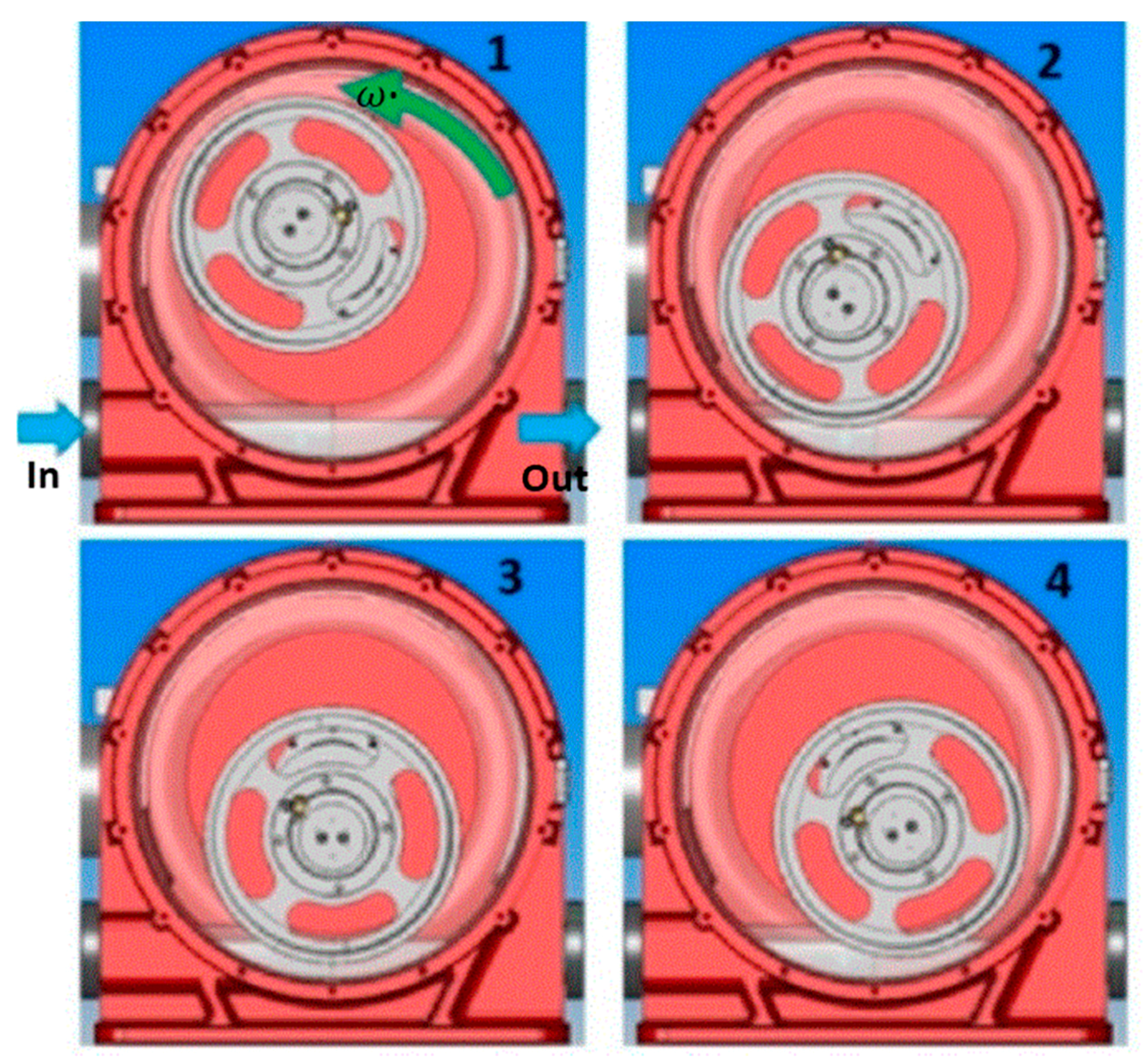
• The internal diameter when the roller squeezed the pipe was reduced by about 87%, (from 32 mm to 4 mm).

Other elements can be added in order to get a more realistic model:

-

Dissipative friction effect between pipe and roller;

-

Roller as deformable material.

From the data results, we found out that it was possible to simulate the singular position in the pipe. Further, when the pipe compressed the inlet and outlet, the pressure had discontinuity that was detected by the numerical model. This discontinuity is due to the geometrical shape of the pipe. As one major advantage, this model, although having minor deficiencies, enables to design new generation peristaltic pump geometries that can have minimal pressure differences during pump operation.

5. Conclusions

The aim of this study was the development of a powerful fluid simulation tool that allowed to optimize the peristaltic pump geometry. The numerical model was able to predict the pump behavior during the operative phase. The simulation data results were compared to the experimental ones. The simulated and experimental cyclic pressure data agreed well with each other; simulated pressure magnitudes were matched, and the maximum difference evaluated between numerical and experimental data obtained was lower than 5%. Therefore, another possible tool application was the geometric optimization of pump housing, roller, and hose parts for developing pressure peak optimized pumps.

Further, in this report, a study of advanced mathematical tools for defective boundary conditions problems for engineering approximations in fluid dynamics was performed. A numerical algorithm was built for the resolution of a laminar flow problem with mean pressure (defective) inlet condition and for the resolution of a steady RANS-based turbulent model with unknown Boundary-Layer height. Therefore, pulsatile flows were examined with FSI and defective analysis by using the commercial software ABAQUS, which is based on a Finite Element method, and then the simulation of the hose pump was performed. For FSI problems, the fluid flow was described by a RANS-based model called RNG k − ϵ in an ALE framework. The FSI-modeling was used for the pumping simulation of the main pump parts interaction, and very good results were obtained.

The FSI model simulations have not been reported vastly in scientific journals and conferences. The few articles do not contain detailed descriptions either of the models or of the results.

As one major goal of this study, this model, although having minor deficiencies, will enable the design of new generation peristaltic pump geometries that can have minimal pressure differences during pump operation.

References

1. Cammarata, A. A novel method to determine position and orientation errors in clearance-affected overconstrained mechanisms. Mech. Mach. Theory 2017, 118, 247–264. [Google Scholar] [CrossRef]
2. Iannone, V.; De Simone, M.C.; Guida, D. Modeling of a DC Gear Motor for Feed-Forward Control Law Design for Unmanned Ground Vehicles. Actuators 2018, in press. [Google Scholar]
3. Cammarata, A.; Angeles, J.; Sinatra, R. Kinetostatic and inertial conditioning of the McGill Schönflies-motion generator. Adv. Mech. Eng. 2010, 2, 186203. [Google Scholar] [CrossRef]
4. De Simone, M.C.; Russo, S.; Rivera, Z.B.; Guida, D. Multibody Model of a UAV in Presence of Wind Fields. In Proceedings of the 2017 International Conference on Control, Artificial Intelligence, Robotics and Optimization (ICCAIRO 2017), Prague, Czech Republic, 20–22 May 2017; pp. 83–88. [Google Scholar]
5. Cammarata, A. Unified formulation for the stiffness analysis of spatial mechanisms. Mech. Mach. Theory 2016, 105, 272–284. [Google Scholar] [CrossRef]
6. De Simone, M.C.; Guida, D. Dry friction influence on structure dynamics. In Proceedings of the 5th ECCOMAS Thematic Conference on Computational Methods in Structural Dynamics and Earthquake Engineering (COMPDYN 2015), Crete Island, Greece, 25–27 May 2015; pp. 4483–4491. [Google Scholar]
7. Yazdanpanh-Ardakani, K.; Niroomand-Oscuii, H. New approach in modeling peristaltic transport of non-newtonian fluid. J. Mech. Med. Biol. 2013, 13, 1350052. [Google Scholar] [CrossRef]
8. Quatrano, A.; De Simone, M.C.; Rivera, Z.B.; Guida, D. Development and implementation of a control system for a retrofitted CNC machine by using Arduino. FME Trans. 2017, 45, 565–571. [Google Scholar] [CrossRef]
9. Cammarata, A.; Lacagnina, M.; Sinatra, R. Dynamic simulations of an airplane-shaped underwater towed vehicle marine. In Proceedings of the 5th International Conference on Computational Methods in Marine Engineering (MARINE 2013), Hamburg, Germany, 29–31 May 2013. [Google Scholar]
10. Barbagallo, R.; Sequenzia, G.; Cammarata, A.; Oliveri, S.M. An integrated approach to design an innovative motorcycle rear suspension with eccentric mechanism. In Advances on Mechanics, Design Engineering and Manufacturing—Lecture Notes in Mechanical Engineering; Springer: Cham, Switzerland, 2017; pp. 609–619. [Google Scholar]
11. Pappalardo, C.M.; Guida, D. On the Lagrange multipliers of the intrinsic constraint equations of rigid multibody mechanical systems. Arch. Appl. Mech. 2018, 88, 419–451. [Google Scholar] [CrossRef]
12. Pappalardo, C.M.; Guida, D. On the Computational Methods for the Dynamic Analysis of Rigid Multibody Mechanical Systems. Machines 2018, 6, 20. [Google Scholar] [CrossRef]
13. Dasic, P. Determination of Reliability of Ceramic Cutting Tools on the basis of Comparative Analysis of Different Functions Distribution. Int. J. Qual. Reliab. Manag. 2001, 18, 431–443. [Google Scholar]
14. Valencia, A.; Villanueva, M. Unsteady flow and mass transfer in models of stenotic arteries considering fluid-structure interaction. Int. Commun. Heat Mass Transf. 2006, 33, 966–975. [Google Scholar] [CrossRef]
15. Reymond, P.; Crosetto, P.; Deparis, S.; Quarteroni, A.; Stergiopulos, N. Physiological simulation of blood flow in the aorta: Comparison of hemodynamic indices as predicted by 3-d fsi, 3-d rigid wall and 1-d models. Med. Eng. Phys. 2013, 35, 784–791. [Google Scholar] [CrossRef] [PubMed]
16. Suito, H.; Takizawa, K.; Huynh, V.Q.; Sze, D.; Ueda, T. Fsi analysis of the blood flow and geometrical characteristics in the thoracic aorta. Comput. Mech. 2014, 54, 1035–1045. [Google Scholar] [CrossRef]
17. Li, H.; Lin, K.; Shahmirzadi, D. Fsi simulations of pulse wave propagation in human abdominal aortic aneurysm: The effects of sac geometry and stiffness. Biomed. Eng. Comput. Biol. 2016, 7, 25–36. [Google Scholar] [CrossRef] [PubMed]
18. Elabbasi, N.; Bergstrom, J.; Brown, S. Fluid-structure interaction analysis of a peristaltic pump. In Proceedings of the 2011 COMSOL Conference, Boston, MA, USA, 13–15 October 2011. [Google Scholar]
19. Zhou, X.; Liang, X.M.; Zhao, G.; Su, Y.; Wang, Y. A new computational fluid dynamics method for in-depth investigation of flow dynamics in roller pump systems. Artif. Organs 2014, 38, E106–E117. [Google Scholar] [CrossRef] [PubMed]
20. Pappalardo, C.M.; Guida, D. Use of the Adjoint Method in the Optimal Control Problem for the Mechanical Vibrations of Nonlinear Systems. Machines 2018, 6, 19. [Google Scholar] [CrossRef]
21. De Simone, M.C.; Rivera, Z.B.; Guida, D. Obstacle avoidance system for unmanned ground vehicles by using ultrasonic sensors. Machines 2018, 6, 18. [Google Scholar] [CrossRef]
22. Pappalardo, C.M.; Guida, D. Dynamic Analysis of Planar Rigid Multibody Systems modelled using Natural Absolute Coordinates. Appl. Comput. Mech. 2018, 12, 73–110. [Google Scholar] [CrossRef]
23. De Simone, M.C.; Guida, D. Modal coupling in presence of dry friction. Machines 2018, 6, 8. [Google Scholar] [CrossRef]
24. Zhai, Y.; Liu, L.; Lu, W.; Li, Y.; Yang, S.; Villecco, F. The application of disturbance observer to propulsion control of sub-mini underwater robot. In Proceedings of the Computational Science and Its Applications (ICCSA 2010), Fukuoka, Japan, 23–26 March 2010; pp. 590–598. [Google Scholar]
25. Pappalardo, C.M.; Guida, D. Control of Nonlinear Vibrations using the Adjoint Method. Meccanica 2017, 52, 2503–2526. [Google Scholar] [CrossRef]
26. De Simone, M.C.; Guida, D. On the development of a low-cost device for retrofitting tracked vehicles for autonomous navigation. In Proceedings of the 23rd Conference of the Italian Association of Theoretical and Applied Mechanics (AIMETA 2017), Salerno, Italy, 4–7 Spetember 2017; pp. 71–82. [Google Scholar]
27. De Simone, M.C.; Guida, D. Control design for an under-actuated UAV model. FME Trans. 2018, 46, 443–452. [Google Scholar] [CrossRef]
28. Barbagallo, R.; Sequenzia, G.; Oliveri, S.M.; Cammarata, A. Dynamics of a high-performance motorcycle by an advanced multibody/control co-simulation. Proc. Inst. Mech. Eng. Part K J. Multi Body Dyn. 2016, 230, 207–221. [Google Scholar] [CrossRef]
29. Pappalardo, C.M.; Guida, D. System Identification Algorithm for Computing the Modal Parameters of Linear Mechanical Systems. Machines 2018, 6, 12. [Google Scholar] [CrossRef]
30. Villecco, F. On the Evaluation of Errors in the Virtual Design of Mechanical Systems. Machines 2018, 6, 36. [Google Scholar] [CrossRef]
31. Donea, J.; Huerta, A.; Ponthot, J.P.; Rodríguez-Ferran, A. Arbitrary Lagrangian_Eulerian Methods; John Wiley & Sons, Ltd.: Hoboken, NJ, USA, 2004. [Google Scholar]
32. Balabel, A.; Dinkler, D. Turbulence models for fluid-structure interaction applications. Emir. J. Eng. Res. 2006, 11, 1–18. [Google Scholar]
33. Barbagallo, R.; Sequenzia, G.; Cammarata, A.; Oliveri, S.M.; Fatuzzo, G. Redesign and multibody simulation of a motorcycle rear suspension with eccentric mechanism. Int. J. Interact. Des. Manuf. 2018, 12, 517–524. [Google Scholar] [CrossRef]
34. De Simone, M.C.; Guida, D. Identification and control of a Unmanned Ground Vehicle by using Arduino. UPB Sci. Bull. Ser. D Mech. Eng. 2018, 80, 141–154. [Google Scholar]
35. Cammarata, A.; Sequenzia, G.; Oliveri, S.M.; Fatuzzo, G. Modified chain algorithm to study planar compliant mechanisms. Int. J. Interact. Des. Manuf. 2016, 10, 191–201. [Google Scholar] [CrossRef]
36. Cammarata, A. Optimized design of a large-workspace 2-DOF parallel robot for solar tracking systems. Mech. Mach. Theory 2015, 83, 175–186. [Google Scholar] [CrossRef]
37. Chakraborty, D.; Prakash, J.R.; Friend, J.; Yeo, L. Fluid-structure interaction in deformable microchannels. Phys. Fluids 2012, 24, 102002. [Google Scholar] [CrossRef] [Green Version]
38. Formato, A.; Guida, D.; Ianniello, D.; Villecco, F.; Lenza, T.L.; Pellegrino, A. Design of Delivery Valve for Hydraulic Pumps. Machines 2018, 6, 44. [Google Scholar] [CrossRef]
39. Sequenzia, G.; Fatuzzo, G.; Oliveri, S.M.; Barbagallo, R. Interactive re-design of a novel variable geometry bicycle saddle to prevent neurological pathologies. Int. J. Interact. Des. Manuf. 2016, 10, 165–172. [Google Scholar] [CrossRef]
40. Guida, D.; Pappalardo, C.M. Control Design of an Active Suspension System for a Quarter-Car Model with Hysteresis. J. Vib. Eng. Technol. 2015, 3, 277–299. [Google Scholar]
41. Ghomshei, M.; Villecco, F.; Porkhial, S.; Pappalardo, M. Complexity in energy policy: A fuzzy logic methodology. In Proceedings of the Sixth International Conference on Fuzzy Systems and Knowledge Discovery (FSKD’09), Tianjin, China, 14–16 August 2009; IEEE: Piscataway, NJ, USA, 2009; pp. 128–131. [Google Scholar]
42. Pappalardo, C.M.; Guida, D. A time-domain system identification numerical procedure for obtaining linear dynamical models of multibody mechanical systems. Arch. Appl. Mech. 2018, 88, 1325–1347. [Google Scholar] [CrossRef]
43. Naviglio, D.; Formato, A.; Scaglione, G.; Montesano, D.; Pellegrino, A.; Villecco, F.; Gallo, M. Study of the Grape Cryo-Maceration Process at Different Temperatures. Foods 2018, 7, 107. [Google Scholar] [CrossRef] [PubMed]
44. Pappalardo, C.M. A Natural Absolute Coordinate Formulation for the Kinematic and Dynamic Analysis of Rigid Multibody Systems. Nonlinear Dyn. 2015, 81, 1841–1869. [Google Scholar] [CrossRef]
45. Cammarata, A.; Lacagnina, M.; Sequenzia, G. Alternative elliptic integral solution to the beam deflection equations for the design of compliant mechanisms. Int. J. Interact. Des. Manuf. 2018, 13, 1–7. [Google Scholar] [CrossRef]
46. Sena, P.; Attianese, P.; Pappalardo, M.; Villecco, F. FIDELITY: Fuzzy Inferential Diagnostic Engine for on-LIne supporT to phYsicians. In International Conference on Biomedical Engineering in Vietnam; Springer: Berlin Heidelberg, 2013. [Google Scholar]
47. Cammarata, A.; Sinatra, R.; Maddio, P.D. A Two-Step Algorithm for the Dynamic Reduction of Flexible Mechanisms. In Proceedings of the 4th IFToMM Symposium on Mechanism Design for Robotics, Udine, Italy, 11–13 Sepember 2018; pp. 25–32. [Google Scholar]
48. Muscat, M.; Cammarata, A.; Maddio, P.D.; Sinatra, R. Design and development of a towfish to monitor marine pollution. Eur. Mediter. J. Environ. Integr. 2018, 3, 11. [Google Scholar] [CrossRef]
49. Cammarata, A.; Lacagnina, M.; Sinatra, R. Closed-form solutions for the inverse kinematics of the Agile Eye with constraint errors on the revolute joint axes. In Proceedings of the IEEE International Conference on Intelligent Robots and Systems, Daejeon, Korea, 9–14 October 2016. [Google Scholar]
50. Bergstrom, J.S. Mechanics of Solid Polymers: Theory and Computational Modeling; William Andrew: Norwich, NY, USA, 2015. [Google Scholar]
Figure 1. Schematic illustration of peristaltic pump.
Machines 07 00050 g001
Figure 2. Mesh of the structural part.
Machines 07 00050 g002
Figure 3. Mesh of the structural part.
Machines 07 00050 g003
Figure 4. Phase 1 of simulation.
Machines 07 00050 g004
Figure 5. Phase 2 of the simulation.
Machines 07 00050 g005
Figure 6. Phase 2 of the simulation; velocity diagram.
Machines 07 00050 g006
Figure 7. Output velocity obtained during the numerical simulation.
Machines 07 00050 g007
Figure 8. Rotation of the roller with period of around 1.1 s.
Machines 07 00050 g008
Figure 9. Von Mises stress at tube outlet.
Machines 07 00050 g009
Figure 10. Pressure data at output of numerical simulation for the considered peristaltic pump.
Machines 07 00050 g010
Figure 11. Experimental pressure data at output of a peristaltic pump.
Machines 07 00050 g011