Dynamics of a Pair of Paramagnetic Janus Particles under a Uniform Magnetic Field and Simple Shear Flow

Abstract

We numerically investigate the dynamics of a pair of circular Janus microparticles immersed in a Newtonian fluid under a simple shear flow and a uniform magnetic field by direct numerical simulation. Using the COMSOL software, we applied the finite element method, based on an arbitrary Lagrangian-Eulerian approach, and analyzed the dynamics of two anisotropic particles (i.e., one-half is paramagnetic, and the other is non-magnetic) due to the center-to-center distance, magnetic field strength, initial particle orientation, and configuration. This article considers two configurations: the LR-configuration (magnetic material is on the left side of the first particle and on the right side of the second particle) and the RL-configuration (magnetic material is on the right side of the first particle and on the left side of the second particle). For both configurations, a critical orientation determines if the particles either attract (below the critical) or repel (above the critical) under a uniform magnetic field. How well the particles form a chain depends on the comparison between the viscous and magnetic forces. For long particle distances, the viscous force separates the particles, and the magnetic force causes them to repel as the particle orientation increases above the configuration’s critical value. As the initial distance decreases, a chain formation is possible at a steady orientation, but is more feasible for the RL-configuration than the LR-configuration under the same circumstances.

1. Introduction

Janus particles, named after the Roman god Janus, are fabricated with two different materials on opposite sides and come in all shapes and forms [1,2,3]. A magnetic Janus particle is an anisotropic particle with a magnetic and a non-magnetic hemisphere, two magnetic hemispheres with different magnetic susceptibilities, or is made up of magnetic or non-magnetic particles with magnetic or non-magnetic caps [4]. The fabrication of Janus particles includes coating and sonicating a whole particle to combine nanoparticles in microfluidic compartments, as well as ultraviolet technology to solidify the Janus particle after forming droplets made out of magnetic and non-magnetic fluids [5,6,7,8,9]. The various important applications of magnetic particles include, but are not necessarily limited to, the creation of complex architectural structures, colloidal superstructures, magnetorheological smart fluids for dampers, valves, and brakes, and biomedical applications such as biosensors, protein detection, and drug delivery systems [9,10,11,12,13,14]. Other advantages of Janus particles in applications include loading florescent nanoparticles, dyes, and drugs [3,15,16,17].

Unlike a dielectric Janus particle chain, which separates due to Brownian motion in the absence of an electric field, magnetic Janus particles separate under demagnetization, giving them an advantage in forming permanent chains and flails [18]. For isotropic particles, chains or flails can form with spherical and elliptical microparticles [19,20]. For anisotropic particles under a magnetic field, staggered chains, double chains, or clusters can be constructed [4,21,22,23,24]. Colloidal superstructures can also be formed under a rotating magnetic field when programmed magnetic Janus particles rotate on their long axis and are used as building blocks with other particles [14]. By applying a simple shear flow, there exists new challenges to study Janus and magnetic/dielectric particles under a uniform magnetic/electric field. In the absence of a magnetic field and under a simple shear flow, particles will collide to form a doublet, are contactless, but orbit periodically around each other (known as a closed orbit), or separate from each other. Previous authors have mentioned additional attributes, including the possibility of the particles forming a chain when under the effects of an electric field or simple shear flow [25,26,27,28,29,30,31,32]. Whether particles orbit around each other or not depends on the initial center-to-center distances and the initial particle orientation. In the presence of a magnetic field, chained isotropic particles can either perform rotational dynamics or rupture under a shear flow [33]. Whether a chain ruptures or rotates depends on the ratio between the viscous force and the magnetic force, also known as the Mason number [33].

Besides using experimentation to study the behavior of Janus particles, numerical simulations apply powerful computer tools to observe the particle-particle interactions and the hydrodynamic and magnetic force effects on the transportation, rotation, and migration behaviors of two or more particles. By applying numerical analyses, we study the effects of hydrodynamic and magnetic forces on the particle dynamics based on many parameters of the numerical model, including the size and shape of the particle, the height, width, and shape of the channel, the shear rate of the fluid, magnetic susceptibilities, the magnetic force between particles, and the strength and direction of the magnetic field.

Even though, to our knowledge, there are no published articles on Janus particles in simple shear flows and under uniform magnetic fields, this research is an important subject for practical applications in science and engineering including experimental and numerical analyses. For experiments, in valves, for example, the viscosity of the fluid increases under a magnetic field, causing a resistance against the velocity of a fluid and based on the fluid’s driving force and its active volume [11,34]. In dampers, the magnetic field strength affects the damping force as shock absorbers by rearranging chains and increasing the yield stress inside the fluid [11,35]. In both cases, however, the ability to retain particle chains and/or clusters (which could consequentially mean the difference between the success and failure of applications) is dependent on the fluid flow (caused by external forces) and the strength of the magnetic field.

As discussed by Anupama et al., under a uniform magnetic field, depending on the particle concentration, single strands (low concentration) or columns (high concentration) are formed in a quiescent fluid [36]. When a low to high shear rate is applied, the effect of the applied magnetic field was analyzed. On the one hand, with a low applied magnetic field, for a low shear rate, the particles are able to react to the flow and rearrange themselves to the initial/equilibrium positions (linear viscoelastic). For a high shear rate, the particles can break and create random structures due to their inability to respond in time (viscoplastic). On the other hand, for a high applied magnetic field, at a low shear rate, the magnetic strength between particles is so high that the flow effect on structured columns is almost negligible. As the shear rate increases, the hydrodynamic force tries to break the bonds between particles, but the columns can either remain intact or reassemble themselves with minimal wall contact. In either of these cases, the particle columns have reportedly deconstructed and reconstructed and will maintain minimal contact with the moving wall.

In numerical studies, Kang et al. successfully analyzed two solid paramagnetic circular particles in a quiescent flow and under a uniform magnetic field, a method that was later applied by Zhang et al. to study two elliptical paramagnetic particles [19,20]. Later, Seong et al. and Kim et al. numerically studied anisotropic circular and elliptical particles under a uniform magnetic field using statistical analysis for their validation [37,38,39]. With many academic literature works leaning towards computer simulations, anisotropic particles in shear flows, and under a uniform magnetic field, we apply the arbitrary Lagrangian-Eulerian (ALE) algorithm for the finite element methods (FEM) and use direct numerical simulation (DNS). The application of this numerical analysis allowed Zhang et al., Cao et al., and Sobecki et al. to compute the dynamics of particles in quiescent, Poiseuille, and simple shear flows for fluid-particle and particle-particle physics [20,40,41,42,43]. Even though our numerical method is different, we nonetheless used Seong et al.’s numerical results to validate our model.

While there have been experimental [4,5,6,7,9,14,18,21,22,23] and numerical [5,9,18,37,38,39] investigations of microscale Janus particle dynamics, our work is the first to study the dynamics of microscale Janus particles in shear flows and under a uniform magnetic field. This can be used for applications in drug delivery, disease diagnosis, and magnetorheological fluids in dampers and pumps. In this article, we focus on a two-dimensional analysis of two anisotropic paramagnetic Janus particles in a simple shear flow and under a uniform magnetic field. For two Janus particles, two configurations are considered: the LR-configuration and the RL-configuration, as well as three parameters: the center-to-center particle distance, the magnetic field strength, and the particle orientation. For two neighboring particles, there exists a particle-particle interaction that affects the surrounding fluid, a viscous force to separate or orbit both particles due to the shear rate, and a magnetic force that allows the particles to either repel and/or attract one another in an attempt to form a chain.

In the validation section, we analyze the dynamics of two circular particles in a simple shear flow in the absence of a magnetic field, the rotational dynamics of a single Janus particle under a uniform magnetic field in a quiescent flow, and the dynamics of two Janus particles under a uniform magnetic field in a quiescent flow. In the first case, depending on the initial particle distance and orientations, under a simple shear flow, the particles will either separate or orbit each other and complete a $2\mathsf{\pi }$ orientation. For the second case, because a circular Janus particle’s magnetic property is anisotropic, the magnetic torque rotates the particle until its hemisphere is parallel to the direction of the magnetic field. Finally, for the third case, the critical orientation of the configurations allows the particles to either attract each other (below the critical orientation) or repel and then attract (above the critical orientation), depending on the initial particle orientation. As the particles are in motion, they affect the surrounding fluid due to the particle-fluid-particle interactions induced by the magnetic force.

Finally, the shear flow and the uniform magnetic field are combined in order to observe how the particles repel or attract due to their orientation and how their relative positions in the fluid domain can affect their dynamics. The particles are shown to repel under the combination between the magnetic and hydrodynamic forces as the orientation of the particles increases by the shear rate above the critical orientation and are further repelled by the magnetic force. In these cases, it is possible to analyze the rate of the particle separation based on the initial orientation and the magnetic field strength. Furthermore, as the initial particle distance decreases, the chain formation is feasible at a stable steady orientation, but occurs more often for one configuration than the other. Although not immensely studied, the particles’ stable steady direction under separation or chain formation and their stable steady orientation are analyzed. A DNS is applied by using an FEM, based on an ALE approach, to analyze the combination among the magnetic field, the simple shear flow, and the particle-particle interaction and to solve the dynamics of the particles and the flow field in a square domain. The hydrodynamic and magnetic forces and torques are computed by a COMSOL FEM solver (5.3a, COMSOL Inc., Burlington, MA, USA) to analyze the orientation and the position displacement motions.

2. Numerical Modeling

2.1. Numerical Setup

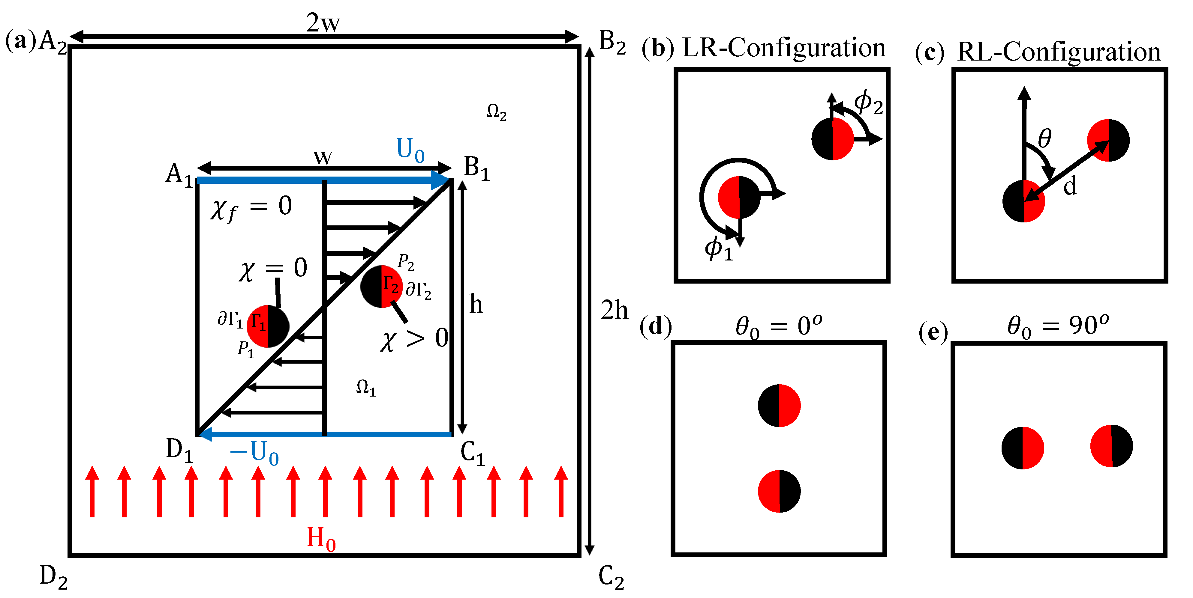
In this article, two equally sized and neutrally buoyant circular Janus particles were placed in a simple shear flow of an incompressible Newtonian fluid, with a density ${\rho }_f$ and a dynamic viscosity ${\eta }_f$, under a uniform magnetic field ${\mathbf{H}}_0$, as seen in Figure 1a. The computational domain consisted of two particle surfaces $\partial {\Gamma }_1$ and $\partial {\Gamma }_2$ and particle domains ${\Gamma }_1$ and ${\Gamma }_2$, where subscripts 1 and 2 represent Particles 1 and 2, respectively. The domains of both Janus particles were equally sectionalized into a paramagnetic side, with a constant susceptibility, and a non-magnetic side, which corresponds to an anisotropic magnetic particle, as seen in similar studies [37]. The anisotropic property of a paramagnetic Janus particle gives it a unique behavior as opposed to its isotropic counterpart. Under a uniform magnetic field, an isotropic paramagnetic particle will not experience a magnetic angular velocity, but a Janus particle rotates until the particle direction (the normal direction to the internal interface) is parallel to the magnetic field direction [37]. Furthermore, a pair of Janus particles’ initial directions can be classified by a configuration, as shown in Figure 1b, the LR-configuration, and Figure 1c, the RL-configuration. The configurations were seen as the initial directions of the particles. For example, the LR-configuration was when Particle 1 had its magnetic half on the left-hand side and ${\varphi }_{1,0}={270}^{\circ }$ (L), whereas Particle 2 had its magnetic half on the right-hand side and ${\varphi }_{2,0}={90}^{\circ }$ (R), and vice-versa for the RL-configuration. The particles were positioned at an orientation, $\theta$, and separated by a center-to-center distance, d. Particle 1’s position was below the origin, whereas Particle 2 was above at $(x_{pi}$, $y_{pi})=\frac{d}{2}(\mp sin\left(\theta \right)$, $\mp cos\left(\theta \right))$, where $i=1$ (“−”) and $i=2$ (“+”) represent Particles 1 and 2, respectively. The Janus particles have an initial orientation, ${\theta }_0$, that is either at or in between ${\theta }_0=0^{\circ }$ (where the particles are vertical to each other) and ${\theta }_0={90}^{\circ }$ (where the particles are horizontal to each other), as shown in Figure 1d,e, respectively.

The computational domain included a fluid domain, ${\Omega }_1$, enclosed by the boundary $A_1{B}_1{C}_1{D}_1$, with the width and height set as $w=h=200$ $\mathsf{\mu }$m, and an air domain, ${\Omega }_2$, enclosed by the boundary $A_2{B}_2{C}_2{D}_2$ with twice the width and height of the fluid domain. The top and bottom boundaries, $A_1{B}_1$ and $D_1{C}_1$, were solid walls with horizontal velocities that were equal, but opposite, thus creating a shear flow. The air domain was used to apply a uniform magnetic field parallel to the y-axis by setting boundaries $B_2{C}_2$ and $D_2{A}_2$ as magnetic insulators. Meanwhile, the $A_2{B}_2$ boundary had a zero magnetic scalar potential, whereas the $C_2{D}_2$ boundary had a magnetic scalar potential of $V_{m0}=H_0\times 2h$. Thus, a uniform magnetic field was developed and was parallel to boundaries $B_2{C}_2$ and $D_2{A}_2$ without a current.

The numerical simulation was initially set up with the wall velocity increasing over time until the shear flow was fully developed. Afterwards, a magnetic field was automatically applied. This ensured that the particles were affected by the shear flow and the magnetic field at approximately the same time.

2.2. Governing Equations: The Magnetostatic Problem

For two Janus particles in a uniform magnetic field, the calculation of a magnetic field was applied in the entire domain without a current. For the entire domain, the magnetic potential is given by the magnetostatic equation:

$$\nabla ·(\mu \nabla \phi )=0,$$

(1)

where $\phi$ is the magnetic scalar potential and $\mathsf{\mu }$ is the magnetic permeability related to the magnetic susceptibility $\chi$ by solving $\mu ={\mu }_0(1+\chi )$, where ${\mu }_0$ is the permeability of free space. The magnetic field intensity, $\mathbf{H}$, and the magnetic flux density, $\mathbf{B}$, are defined by the magnetic scalar potential and permeability $\mathbf{H}=-\nabla \phi$ and $\mathbf{B}=\mu \mathbf{H}$, respectively.

It should be mentioned that for an anisotropic particle in a non-magnetic fluid, there are two discontinuities regarding the magnetic permeability. The first discontinuity is across the interface between the fluid and the outer boundary of the magnetic domain of the particle. The second discontinuity is across the boundary between the magnetic and non-magnetic domains inside the particle. This gives a non-uniform magnetic field and permeability inside a Janus particle. Thus, $\mu ={\mu }_0$ inside the fluid, air, and non-magnetic particle domains, and $\mu ={\mu }_0(1+\chi )$ in the magnetic particle domain. After finding the magnetic field intensity and flux density, without a current, the magnetic scalar potential satisfies the governing Maxwell equations, independent of any boundary conditions:

$$\nabla \times \mathbf{H}=\mathbf{0},$$

(2)

$$\nabla ·\mathbf{B}=0.$$

(3)

The pair of Janus particles are assumed to be in a Stokes flow regime, and the inertia of the particles is considered neglected because the Reynolds number is low. These assumptions are usually applied in microscale flows for a Reynolds number less than one and for microscale particles (spherical and non-spherical) [33,40,42,43,44,45]. Thus, under a Stokes flow regime and a uniform magnetic field, the flow is governed by the continuity and the momentum balance equations, and the particles are governed by Newton’s second law:

$$\nabla ·\mathbf{u}=\mathbf{0}$$

(4)

$$\nabla ·\mathbf{œ}+\nabla ·{\mathbf{T}}_m=\mathbf{0},$$

(5)

where $\mathbf{u}$ is the fluid velocity, $\mathbf{œ}=-p\mathbf{I}+{\eta }_f(\nabla \mathbf{u}+{(\nabla \mathbf{u})}^T)$ is the Cauchy stress tensor, and ${\mathbf{T}}_m=\mu (\mathbf{H}\mathbf{H}-H^2\mathbf{I}/2)$ is the Maxwell stress tensor. The stress tensors are defined by the pressure, p, the viscosity, ${\eta }_f$, the identity tensor $\mathbf{I}$, and $H^2=\mathbf{H}·\mathbf{H}$. The magnetic force between the Janus particles is calculated by taking the divergence of the Maxwell tensor and is added to the momentum balance equation.

2.3. Governing Equations: The Flow Problem

In addition to the continuity equation, the fluid flow $\mathbf{u}$ is governed by the Navier–Stokes equation with a no-slip condition on walls $A_1{B}_1$ and $D_1{C}_1$ and with zero normal pressure at boundaries $D_1{A}_1$ and $B_1{C}_1$ as shown in Figure 1a:

$${\rho }_f[\frac{\partial \mathbf{u}}{\partial t}+(\mathbf{u}·\nabla )\mathbf{u}]=\nabla ·{\eta }_f(\nabla \mathbf{u}+{(\nabla \mathbf{u})}^T)+\nabla ·{\mathbf{T}}_m,$$

(6)

where t is time. In a Stokes flow, if we non-dimensionalize the Navier–Stokes equation, the Reynolds number would be on the left-hand side of the equation. Therefore, as the Reynolds number approaches zero, the acceleration term, $\frac{\partial \mathbf{u}}{\partial t}$, and the inertial term, $(\mathbf{u}·\nabla )\mathbf{u}$, would disappear. The velocity of the fluid, $\mathbf{u}$, is also governed by the constraint for the rigid body motion on the surface of the ith particle. The fluid velocity is based on the position on the ith particle’s surface, $\mathbf{x}$, along with the ith particle’s angular velocity ${\omega }_i$, the ith particle’s center of mass position ${\mathbf{x}}_i=(x_i,y_i)$, and the ith particle’s translational velocity ${\mathbf{u}}_i$:

$$\mathbf{u}={\mathbf{u}}_i+{\omega }_i\times \left(\mathbf{x}-{\mathbf{x}}_i\right),on\partial {\Gamma }_i\left(t\right)(i=1,2,...,N),$$

(7)

$$\mathbf{u}=\dot{\gamma }h/2on{A}_1{B}_1,$$

(8)

$$\mathbf{u}=-\dot{\gamma }h/2on{C}_1{D}_1,$$

(9)

where the latter two equations are the fluid velocity on the channel walls $A_1{B}_1$ and $C_1{D}_1$ where $\dot{\gamma }$ is the shear rate of the fluid.

Since there is also a no-slip condition on the surface of the particles, the fluid velocity on the particles’ surfaces is a function of the particle translation velocity at their positions and rotation velocity at their directions ${\varphi }_i$ and at time t:

$$\frac{d(x_i,y_i)}{dt}={\mathbf{u}}_i,$$

(10)

$$(x_i\left(0\right),y_i\left(0\right))=(x_{i,0},y_{i,0}),$$

(11)

$$\frac{d{\varphi }_i}{dt}={\omega }_i,$$

(12)

$${\varphi }_i\left(0\right)={\varphi }_{i,0},$$

(13)

where $(x_{i,0},y_{i,0})$ and ${\varphi }_{i,0}$ are the initial positions and the initial direction of the $ith$ particle, respectively. Finally, we add the balance equations for the forces and torques acting on both particles in order to calculate the rigid body motions. Assuming that inertia is absent, we have two balance equations that are integrated over the ith particle’s surface:

$${\mathbf{F}}_i={\int }_{\partial {\Gamma }_i}(\mathbf{œ}+{\mathbf{T}}_m)·\mathbf{n}dS=\mathbf{0},$$

(14)

$${\mathbf{T}}_i={\int }_{\partial {\Gamma }_i}{\mathbf{r}}_i\times [(\mathbf{œ}+{\mathbf{T}}_m)·\mathbf{n}]dS=\mathbf{0},$$

(15)

where ${\mathbf{F}}_i$ is the sum of the hydrodynamic and magnetic forces to calculate the particles’ velocity and ${\mathbf{T}}_i$ is the sum of the hydrodynamic and magnetic torques to calculate the particles’ angular velocity over the surface of the particles at time t.

2.4. Material Properties and Dimensionless Scale

In the following simulation results, the fluid in domain ${\Omega }_1$ is incompressible and Newtonian, and its property is a water-based material with a density and dynamic viscosity of 1000 kg/m${}^3$ and $1.002\times {10}^{-3}$ Pa·s, respectively. The material in domain ${\Omega }_2$ is air. Both domains are square shaped with the side lengths of ${\Omega }_2$ twice that of ${\Omega }_1$ and $w=h=200$ $\mathsf{\mu }$m. The velocities of the top and bottom walls are $U=2$ cm/s and $U=-2$ cm/s, respectively; thus, the shear rate is $\dot{\gamma }=200$ 1/s. The Janus particles have a density of about 1100 kg/m${}^3$ and a radius of $r=3.5$ $\mathsf{\mu }$m. The magnetic susceptibility for one-half of the Janus particle, the air, and the fluid is $\chi =0$, whereas the other half of the Janus particles has a susceptibility of $\chi =1$ [37].

Throughout this article, all data shown were non-dimensionalized. Any unit of length will be dimensionless by dividing by the particle radius. Thus, the center-to-center distance was set as $d^{*}=d/r$, and the initial and time-dependent particle positions became $(x_{i,0}^{*},y_{i,0}^{*})=(x_{i,0},y_{i,0})/r$ and $(x_i^{*},y_i^{*})=(x_i,y_i)/r$, respectively. There were also two dimensionless times. With moving walls, the dimensionless time was set as $t^{*}=t\dot{\gamma }$, and without moving walls, the dimensionless time was set with the magnetic time scale $t_m=\frac{{\eta }_f}{{\mu }_0{\beta }^2{H}_0^2}$, where $\beta =\frac{{\chi }_p}{3+{\chi }_p}$[19,20,33,37,38,39]. Furthermore, to compare the strength of the viscous and the magnetic forces, one can calculate the Mason number $M_n=\frac{{\eta }_f\dot{\gamma }}{{\mu }_0{\beta }^2{H}_0^2}$, where a lower Mason number value indicates that the magnetic force is more dominant than the viscous force and can allow particles to form a chain or stay magnetized, whereas a higher Mason number has the opposite effect. Since we will only focus on two magnetic field strengths and only one magnetic susceptibility for the magnetic domain of the Janus particle, we will not focus on the Mason number as Kang et al. demonstrated [33]. The strength between the magnetic and viscous forces, however, was analyzed due to the distances of the particles, the magnetic field strength, and the particle orientations.

3. Validation of the Numerical Simulation

The rotation and migration dynamics of two anisotropic paramagnetic Janus particles are affected by the hydrodynamic and magnetic forces and torques. With the existence of two circular particles near each other, particle-particle and particle-fluid interactions become important phenomena to consider the effect on fluid flow, forces, and torques in addition to channel size, particle orientation, distance, and direction. Given the parameters of the channel and the particles, we used a direct numerical simulation (DNS) from the finite element method (FEM) and an arbitrary Lagrangian-Eulerian (ALE) method for the coupling of particle-particle interactions, fluid flow, and the uniform magnetic field. Our simulations were solved by numerical modeling using a commercial FEM solver, COMSOL Multiphysics. Here, we meshed inside and outside of the particles in a time-dependent solver for a particle-particle and particle-fluid interaction model. The simple shear flow was gradually increased using the step function, and at the same time, a piecewise function was used to activate the uniform magnetic field. In our model, we used a quadratic triangular mesh inside all domains, where the total number of meshes was 27,706 elements where the Janus particles had 6750 domain elements and 368 surface elements, the fluid domain has 16,234 elements, and the air domain has 4722 elements. Furthermore, we used a time step of $\Delta t=1e-5$s.

In this section, we quantitatively validate our numerical simulations, as shown in Figure 2. We validate the dynamics for two circular particles in a simple shear flow without a magnetic field with Darabaner et al. in Figure 2a, the rotational dynamics of a single Janus particle in Figure 2b, and the dynamics of two Janus particles in Figure 2c,d [25]. The latter three are Janus particles under a uniform magnetic field without a simple shear flow and were validated with Seong et al. [37].

Shown in Figure 2a are the results of a pair of particles in a simple shear flow without a magnetic field, an initial distance of $d_0^{*}=2.4$, and initial particle orientations of ${\theta }_0=0^{\circ }$ and ${\theta }_0={90}^{\circ }$. As can be seen, the particles with an initial orientation of ${\theta }_0=0^{\circ }$ separate, and their positions are slightly displaced as they are carried by the simple shear flow. On the other hand, for ${\theta }_0={90}^{\circ }$, the particles complete a periodic $2\mathsf{\pi }$ orientation around each other and end at almost the exact position where they began. At the end of the $2\mathsf{\pi }$ orientation, the error for each particle’s begin and end positions are $0.5$ percent for Particle 1 and $0.25$ percent for Particle 2. Therefore, our model is in quantitative agreement with Darabaner et al. [25].

Secondly, a single Janus particles was compared to Seong et al. for validation [37]. Shown in Figure 2b are the angular velocity ${\omega }^{*}=\omega t_m$ and direction of the Janus particle, $\varphi$, over a period of dimensionless time $t^{*}=t/t_m$. The initial direction of the particle was set to ${\varphi }_0=0.1^{\circ }$, and the magnetic strength was $H_0=5000$ A/m. As can be seen, the minimum angular velocity occurs at the particle directions $\varphi =0^{\circ }$ and $\varphi ={90}^{\circ }$, and the maximum angular velocity occurs at around $\varphi ={45}^{\circ }$. The results were thus in agreement with Seong et al.

Finally, the LR- and RL-configurations under a magnetic field strength at $H_0=5000$ A/m and at an initial distance $d^{*}=4$ were also validated with Seong et al., as shown in Figure 2c for the LR-configuration and Figure 2d for the RL-configuration. The initial particle orientations were ${\theta }_0=0^{\circ }$, ${\theta }_0={20}^{\circ }$, and ${\theta }_0={45}^{\circ }$ for the LR-configuration and ${\theta }_0=0^{\circ }$, ${\theta }_0={20}^{\circ }$, and ${\theta }_0={53}^{\circ }$ for the RL-configuration. The critical orientations represent a boundary between whether the particles will initially attract each other or if they will repel then attract and were approximately ${\theta }_{c,LR}\approx 32.5^{\circ }$ and ${\theta }_{c,RL}\approx 53.5^{\circ }$[37]. As can be seen in Figure 2c, for the LR-configuration, the particles attract at ${\theta }_0=0^{\circ }$ and ${\theta }_0={20}^{\circ }$, whereas the particles first repel and then attract at ${\theta }_0={45}^{\circ }$. Similarly, in Figure 2c, for the RL-configuration, the particles attract at ${\theta }_0=0^{\circ }$ and ${\theta }_0={20}^{\circ }$, whereas the particles first repel and then attract at ${\theta }_0={53}^{\circ }$. Once again, the numerical results (shown in lines) quantitatively agreed with the previous authors’ results (shown in symbols), and we used a total number of around 27,000 meshes and a time step of $1e-5$s.

4. Results and Discussion

In this section, the magnetic field was applied at the strengths $H_0=0$ A/m (absent magnetic regime), $H_0=5000$ A/m (moderate magnetic regime), and $H_0=$ 10,000 A/m (strong magnetic regime). Both particles were initially separated at $d_0^{*}=2.4$, $d_0^{*}=3.2$, and $d_0^{*}=4.0$ and at initial particle orientations ${\theta }_0=0^{\circ }$, ${\theta }_0={25}^{\circ }$, ${\theta }_0={65}^{\circ }$, and ${\theta }_0={90}^{\circ }$. In this case, we combined the importance of the distances and orientations from our simple shear flow and the magnetic field strengths by using two particle orientations that were below and above the critical values for both configurations. For the rest of this investigation, not only were the magnetic and viscous forces evaluated, but the behaviors of the LR- and RL-configurations were also compared since they had different critical orientations. The comparisons included how fast particles would separate, the orientation and the stable steady direction, and their positions in the fluid domain. If the magnetic force was strong enough, the particles would form a chain at a stable steady orientation ${\theta }^{LR,ss}$ and/or ${\theta }^{RL,ss}$, as shown in

Table 1. Values for the stable steady orientations ${\theta }^{LR,ss}$ for the LR-configuration. The absence of a value, N/A, depicts that the viscous force is more dominant than the magnetic force. The initial distance $d_0^{*}=4.0$ is not included because a chain does not form.

${\mathit{\theta }}_0$	${\mathit{d}}_0^{*}=2.4$	${\mathit{d}}_0^{*}=2.4$	${\mathit{d}}_0^{*}=3.2$	${\mathit{d}}_0^{*}=3.2$
	${\mathit{H}}_0=5000$ A/m	${\mathit{H}}_0=$ 10,000 A/m	${\mathit{H}}_0=5000$ A/m	${\mathit{H}}_0=$ 10,000 A/m
$0^{\circ }$	N/A	${342}^{\circ }$	N/A	$341.{60}^{\circ }$
${25}^{\circ }$	N/A	${342}^{\circ }$	N/A	N/A
${65}^{\circ }$	N/A	N/A	N/A	N/A
${90}^{\circ }$	N/A	N/A	N/A	N/A

and

Table 2. Values for the stable steady orientations ${\theta }^{RL,ss}$ for the RL-configuration. The absence of a value, N/A, depicts that the viscous force is more dominant than the magnetic force. The initial distance $d_0^{*}=4.0$ is not included because a chain does not form.

${\mathit{\theta }}_0$	${\mathit{d}}_0^{*}=2.4$	${\mathit{d}}_0^{*}=2.4$	${\mathit{d}}_0^{*}=3.2$	${\mathit{d}}_0^{*}=3.2$
	${\mathit{H}}_0=5000$ A/m	${\mathit{H}}_0=$ 10,000 A/m	${\mathit{H}}_0=5000$ A/m	${\mathit{H}}_0=$ 10,000 A/m
$0^{\circ }$	${33}^{\circ }$	${25}^{\circ }$	N/A	$24.{86}^{\circ }$
${25}^{\circ }$	${33}^{\circ }$	${25}^{\circ }$	N/A	$24.{86}^{\circ }$
${65}^{\circ }$	N/A	${25}^{\circ }$	N/A	N/A
${90}^{\circ }$	N/A	N/A	N/A	N/A

in Section 4.3.

4.1. The LR-Configuration

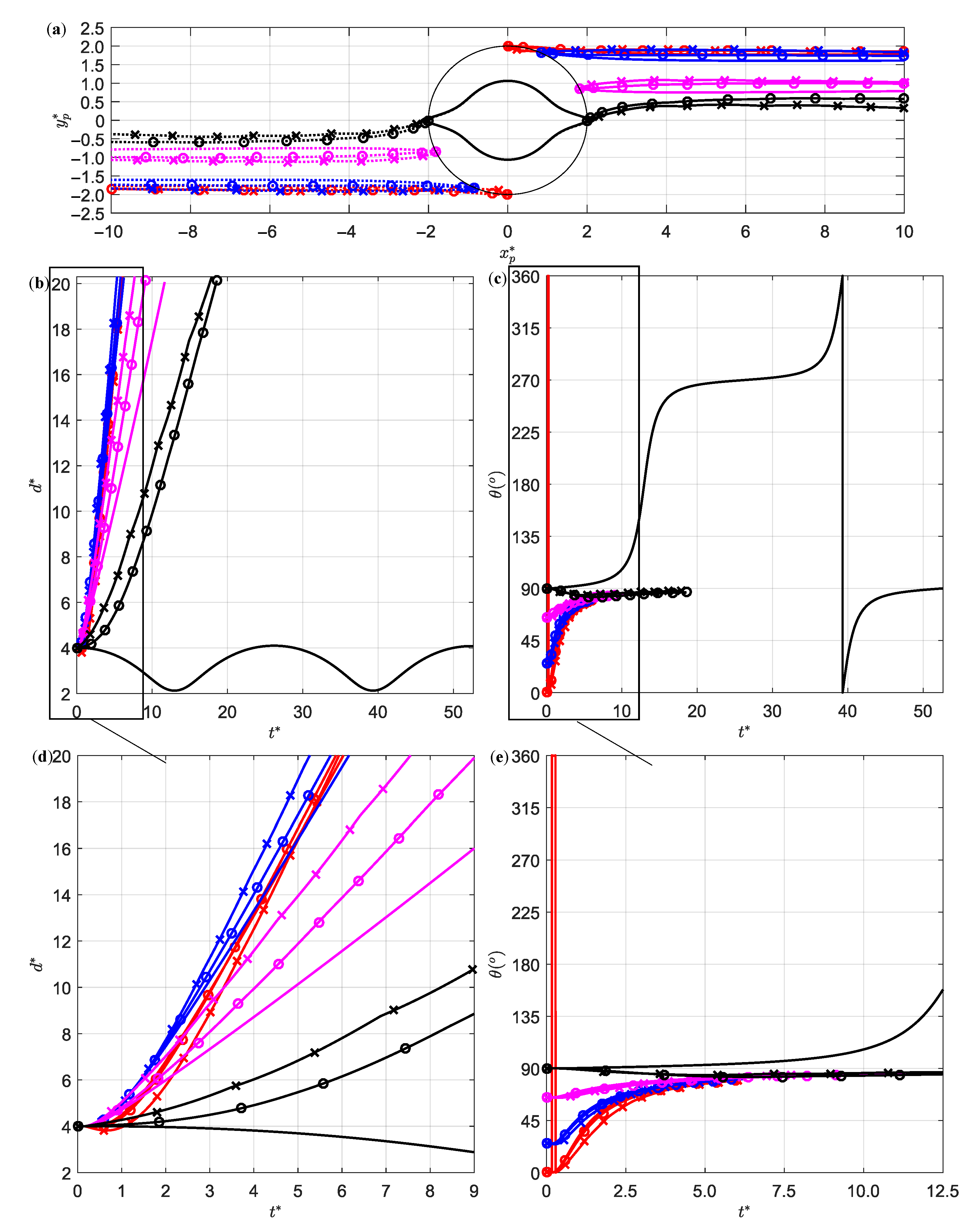
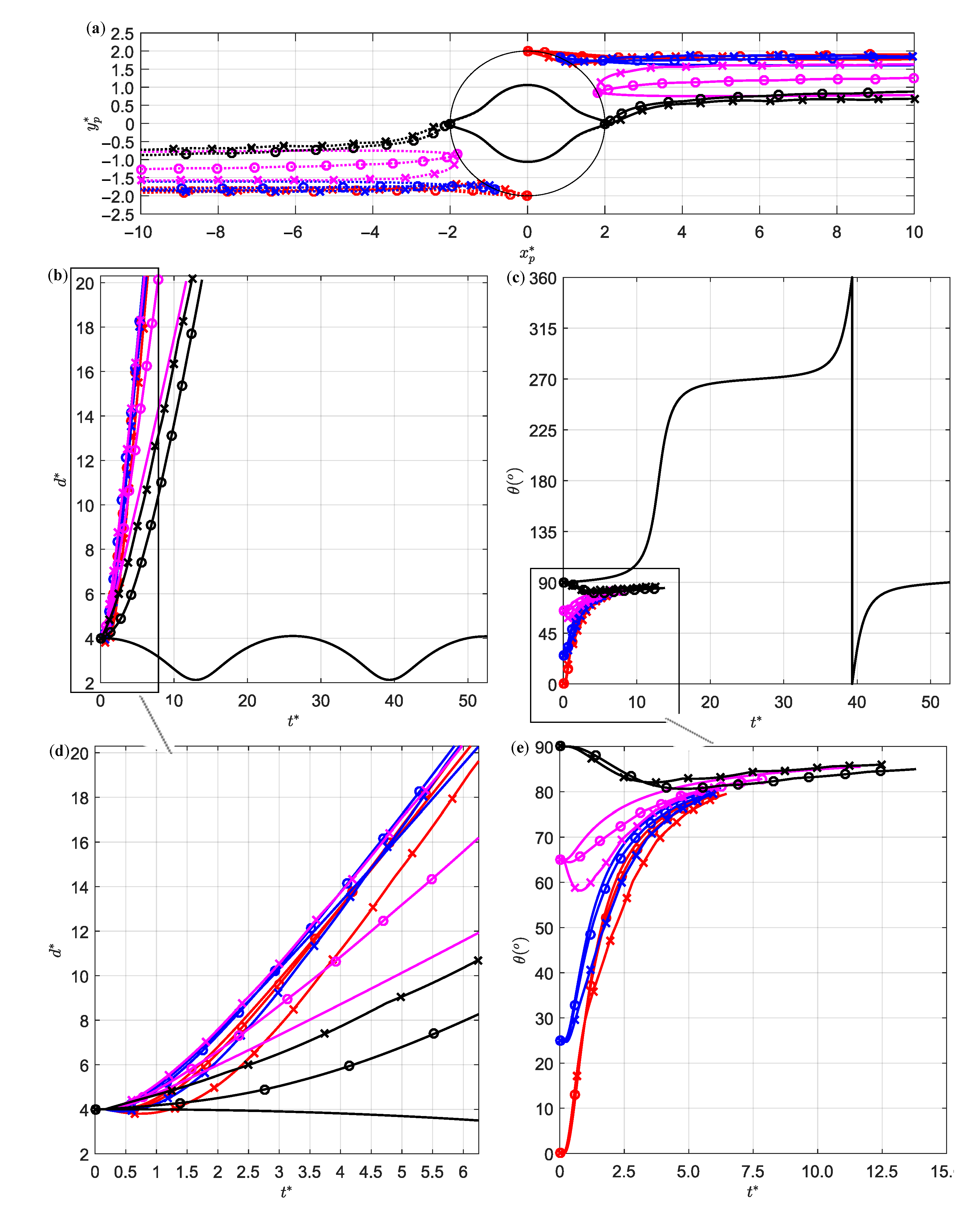
The particle dynamics for the LR-configuration at initial distances $d_0^{*}=4.0$, $d_0^{*}=3.2$, and $d_0^{*}=2.4$ are shown in Figure 3, Figure 4, and Figure 5, respectively. As seen in Figure 3a,b,d, the viscous forces were stronger than the magnetic forces, and the particle distances would increase over time, but at different rates. The only exception was the initial particle orientation at ${\theta }_0={90}^{\circ }$ and $H_0=0$ A/m, where the particle distance oscillated, as seen in Figure 3b,d, and the particles would orbit around each other, as seen in Figure 3a,c,e. For ${\theta }_0=0^{\circ }$, the distance of both particles under a magnetic field strength $H_0=5000$ A/m separated faster than at $H_0=0$ A/m and $H_0=$ 10,000 A/m. When the magnetic field strength was $H_0=$ 10,000 A/m, the particles would initially attract each other towards the origin of the fluid domain before the viscous force overcame the magnetic force and separated the particles. On the other hand, for other magnetic field strengths, the particles’ positions were initially further from the origin, which explains the initial faster separation rate before the $H_0=$ 10,000 A/m line surpassed the $H_0=0$ A/m line in Figure 3b,d. The behavior can be explained by the strength of the magnetic field and the shear flow. At some point in time, the particle orientation became greater than the critical orientation, ${\theta }^{LR,ss}\approx {32}^{\circ }$, and the particles repelled each other, resulting in a greater orientation rate, as shown in Figure 3c,e. For all other initial particle orientations, the particles under the magnetic field strength $H_0=$ 10,000 A/m would repel each other faster than the lesser magnetic strengths. Under a uniform magnetic field strength greater than zero, the following particle orientations are given from the fastest to slowest separation: ${\theta }_0={25}^{\circ }$, ${\theta }_0=0^{\circ }$, ${\theta }_0={65}^{\circ }$, ${\theta }_0={90}^{\circ }$. In Figure 3c,e, we noticed that since the magnetic force was initially stronger for ${\theta }_0=0^{\circ }$ and $H_0=$ 10,000 A/m, the particle orientation would rotate backwards before the viscous force overcame the magnetic force. For particles with an initial orientation less than ${\theta }_0={90}^{\circ }$, the particle orientation would monotonically increase over time, with the lesser magnetic strengths initially allowing a faster orientation rate before the larger magnetic field strengths surpassed it. On the other hand, for the initial orientation ${\theta }_0={90}^{\circ }$, the orientation of both particles under a uniform magnetic field would decrease monotonically and then increase. Obviously, if the fluid domain was an infinite rectangular domain, the particle distance would increase over time, and the particle orientation would approach $\theta ={90}^{\circ }$.

Next, the particle dynamics for $d_0^{*}=3.2$ in Figure 4 were observed. As can be seen, in most cases, the particles separated because either the viscous force was stronger than the magnetic force or the particles would initially repel each other and be further separated by the shear flow. The only exception was when the particles formed a chain at a stable steady orientation, ${\theta }^{LR,ss}$, shown in Figure 4c,e, at ${\theta }_0=0^{\circ }$ and under the magnetic field strength $H_0=$ 10,000 A/m. As seen in Figure 4b,d, the initial orientation ${\theta }_0={25}^{\circ }$ had a faster separation rate because the particles were initially attracting each other. The shear rate, however, forced the particle orientation to increase above the critical orientation, as seen in Figure 4c,e. At this point, the particles repelled each other, and their positions drifted further from the origin. The latter orientations had a slower separation rate with the initial orientation ${\theta }_0={65}^{\circ }$ separating faster than ${\theta }_0={90}^{\circ }$. Similar to the initial separation at $d_0^{*}=4.0$, the particles with an initial distance of $d_0^{*}=3.2$ under a magnetic field strength of $H_0=5000$ A/m would initially attempt to attract each other under a strong magnetic regime before the viscous force separated them, as seen in Figure 4c,e.

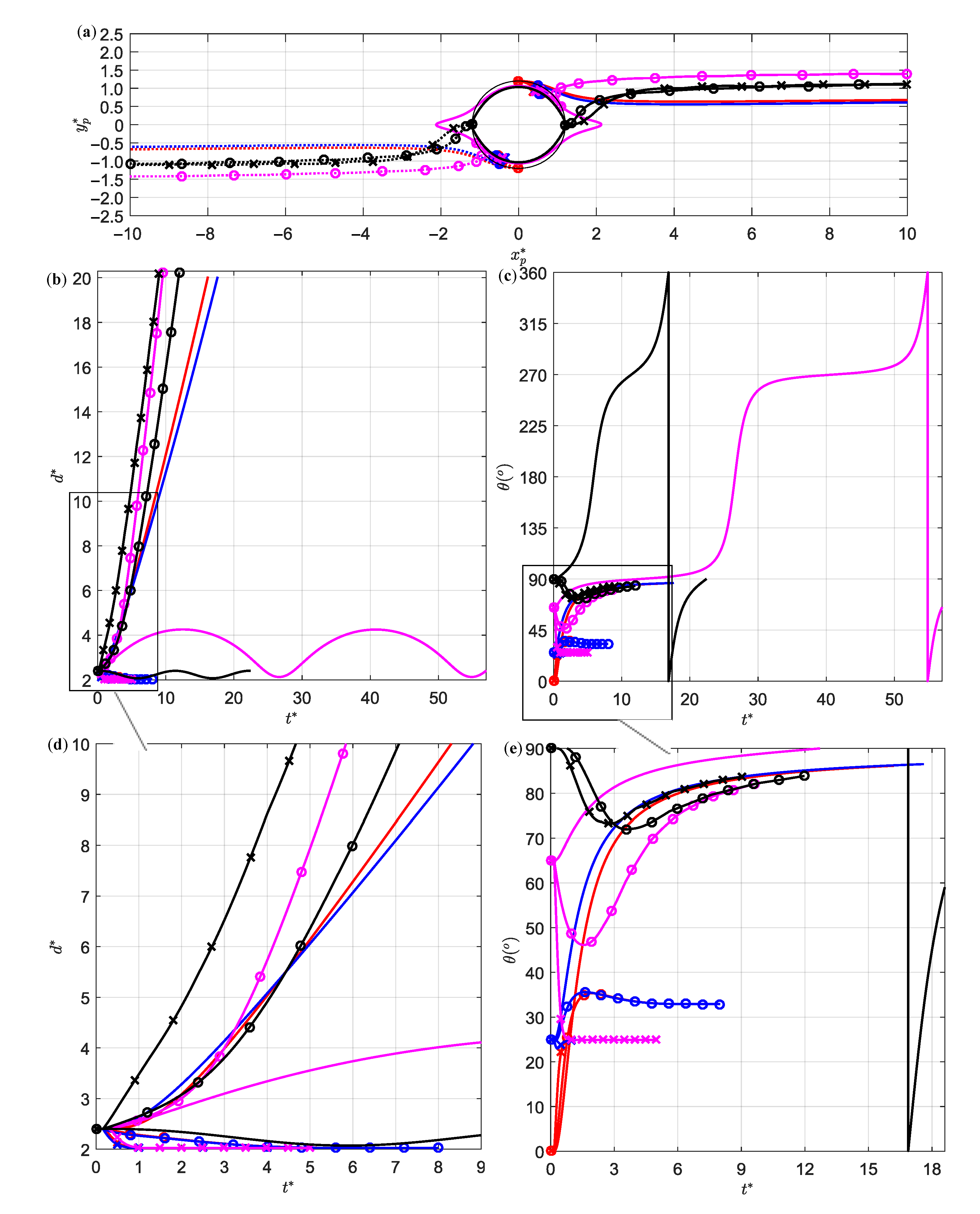
Finally, the particle dynamics were observed at $d_0^{*}=2.4$, as seen in Figure 5. In Figure 5a,b,d, the magnetic force was stronger than the viscous force for the initial orientations ${\theta }_0=0^{\circ }$ and ${\theta }_0={25}^{\circ }$ at the strength $H_0=$ 10,000 A/m, and the particle distances decreased until a chain was formed. In all other cases, however, the viscous force was stronger than the magnetic, and thus, the particle distances increased at different rates. The only exception was when the particles completed periodic orientations at ${\theta }_0={65}^{\circ }$ and ${\theta }_0={90}^{\circ }$ in the absence of a magnetic field. At the magnetic field strength $H_0=$ 10,000 A/m, the particles separated faster at the initial particle orientation of ${\theta }_0={65}^{\circ }$ than all other cases, including ${\theta }_0={90}^{\circ }$ at the same magnetic field strength. For the magnetic field strength $H_0=5000$ A/m, the following particle orientations are given from the fastest separation to the slowest: ${\theta }_0={25}^{\circ }$, ${\theta }_0={65}^{\circ }$, ${\theta }_0=0^{\circ }$, and ${\theta }_0={90}^{\circ }$. In fact, the particle separation rate for $H_0=5000$ A/m and ${\theta }_0=0^{\circ }$ was initially slower because the particle orientation rotated backwards, as seen in Figure 5c,e, before monotonically increasing. Similar to other initial distances and under a uniform magnetic field, the particles with an initial orientation ${\theta }_0={90}^{\circ }$ monotonically decreased and then increased. The rates of the orientation decreasing and/or increasing, the rate of the periodic orientation, and whether or not a chain forms depended on the particles’ positions in the fluid domain and their initial orientations. When the particles were further away from the origin, the particles separated faster and approached $\theta ={90}^{\circ }$.

For an LR-configuration, it was difficult to form a particle chain under a uniform magnetic field and in a simple shear flow. In many cases, the strength of the viscous force is greater than the magnetic force, and the particle separation and orientation rates depend on the particle dynamics at different magnetic field strengths and at initial orientations. For ${\theta }_0={65}^{\circ }$ and ${\theta }_0={90}^{\circ }$, even at the closest distance simulated, the particles repelled each other, and their orientation varied at different particle positions in the fluid domain. In a couple of cases, the magnetic force was initially greater than the viscous force, and the particle orientation rotated backwards, and they attracted each other; however, over time, the viscous force broke that attraction. Additionally, their orientation would increase above the critical orientation, and the particles repelled each other. In a strong magnetic regime, the particles formed a staggered chain near the origin at ${\theta }^{LR,ss}$. At initial orientations, ${\theta }_0=0^{\circ }$ and ${\theta }_0={25}^{\circ }$, the Janus particles with an initial distance of $d_0^{*}=4.0$ had a faster separation and orientation rate because the particles were initially further away from the origin of the fluid domain. On the other hand, as the initial distance decreased, the chain formation became more feasible.

4.2. The RL-Configuration

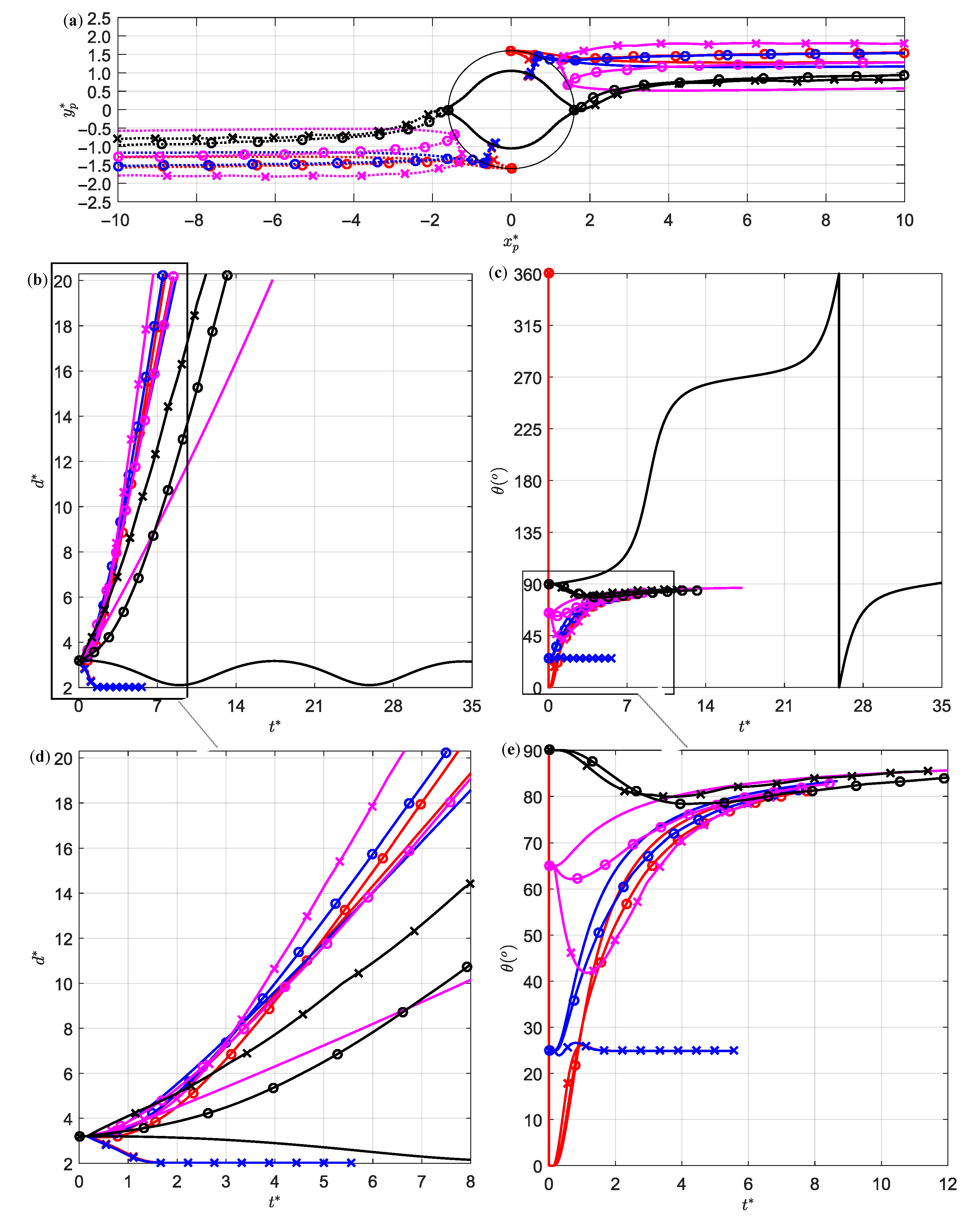
The particle dynamics for the RL-configuration at initial distances $d_0^{*}=4.0$, $d_0^{*}=3.2$, and $d_0^{*}=2.4$ are shown in Figure 6, Figure 7, and Figure 8, respectively. Similar to the LR-configuration, at $d_0^{*}=4.0$, in Figure 6a,b,d, the viscous force was stronger than the magnetic force, and the particles distances would increase at different rates except for ${\theta }_0={90}^{\circ }$ and $H_0=0$ A/m. For ${\theta }_0=0^{\circ }$, both particles under a magnetic field strength $H_0=5000$ A/m separated faster than at $H_0=0$ A/m and $H_0=$ 10,000 A/m. On the other hand, at ${\theta }_0={25}^{\circ }$, the particles initially separated faster when $H_0=0$ A/m and $H_0=5000$ A/m than for $H_0=$ 10,000 A/m, but the $H_0=$ 10,000 A/m line surpassed the $H_0=0$ A/m line. Eventually, the particle orientation was greater than the critical for the RL-configuration, and the particles repelled each other, as shown in Figure 6c. For all other initial particle orientations, particles under the strongest magnetic field would repulse each other faster than the lesser magnetic strengths. Under a uniform magnetic field greater than zero, the following particle orientations were given from the fastest separation to the slowest: ${\theta }_0={25}^{\circ }$, ${\theta }_0=0^{\circ }$, ${\theta }_0={65}^{\circ }$, ${\theta }_0={90}^{\circ }$. In Figure 6c,e, since the magnetic force was initially stronger for ${\theta }_0=0^{\circ }$ and $H_0=$ 10,000 A/m, the particle orientation rotated backwards before separating under the viscous force. For particles with an initial orientation less than ${\theta }_0={90}^{\circ }$, the particle orientation monotonically increased, with the lesser magnetic strengths initially having a faster orientation rate before being surpassed by larger magnetic field strengths. For ${\theta }_0={90}^{\circ }$, both particles under the magnetic field strengths of $H_0=5000$ A/m and $H_0=$ 10,000 A/m would decrease monotonically and then increase.

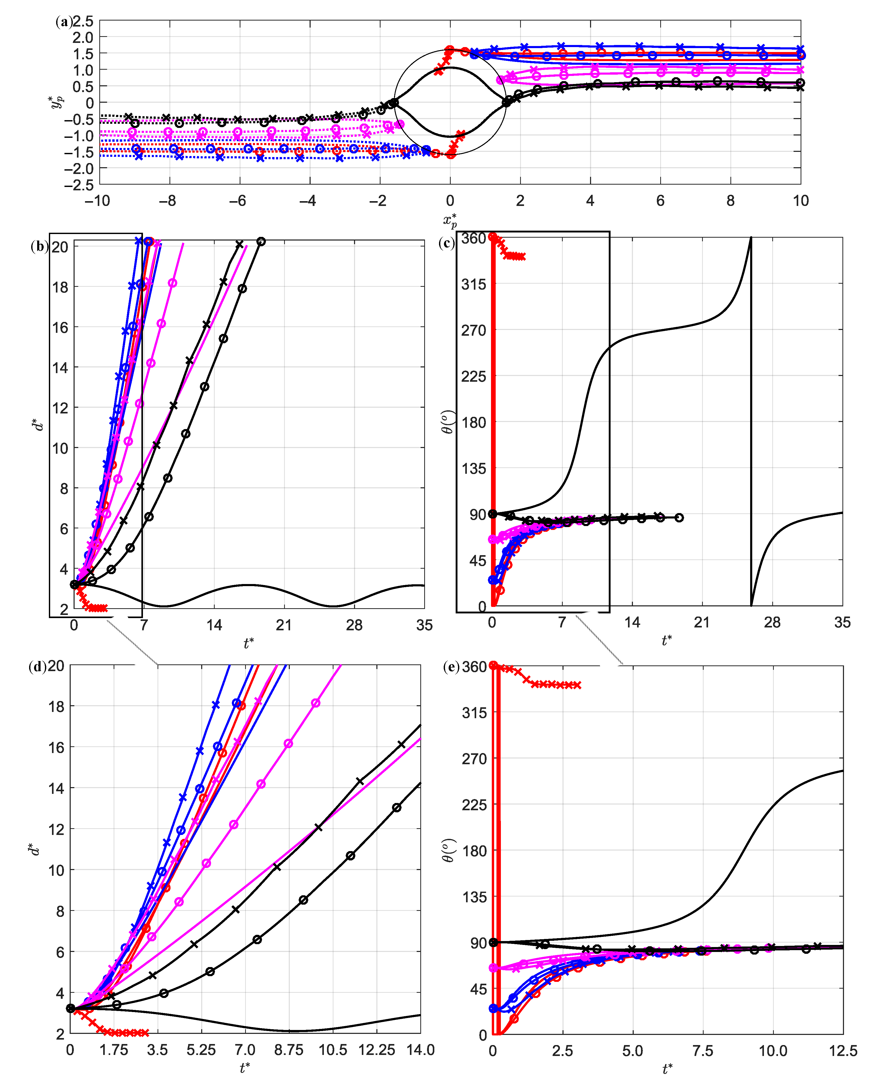
Next, the particle dynamics were observed at an initial distance of $d_0^{*}=3.2$, as seen in Figure 7, where chains were formed at ${\theta }^{RL,ss}$ for initial orientations ${\theta }_0=0^{\circ }$, ${\theta }_0={25}^{\circ }$ at the magnetic field strength $H_0=$ 10,000 A/m. At the magnetic field strength $H_0=5000$ A/m, the viscous force was stronger than the magnetic force, and particle distances and orientations increased for ${\theta }_0=0^{\circ }$ and ${\theta }_0={25}^{\circ }$. On the other hand, for ${\theta }_0={65}^{\circ }$ and ${\theta }_0={90}^{\circ }$ and in the presence of a magnetic field, even though their distances were increasing, their orientations first decreased and then increased monotonically. For an additional observation in Figure 7a, both moderate and strong magnetic regimes caused the particles to repel. Interestingly enough, for ${\theta }_0={65}^{\circ }$ and $H_0=$ 10,000 A/m, the particles initially repelled each other, and the magnetic field attempted to attract the particles below the critical orientation. Eventually, the particles’ positions inside the fluid domain were far away from the origin to where the viscous force broke the attraction. Due to the shear flow, the particle orientation was eventually above the critical orientation, and the particles repelled each other again under the magnetic field. Once again, for the magnetic field strength $H_0=5000$ A/m, a faster particle separation occurred at ${\theta }_0={25}^{\circ }$, and thus, its particle orientation rate was greater than for ${\theta }_0=0^{\circ }$.

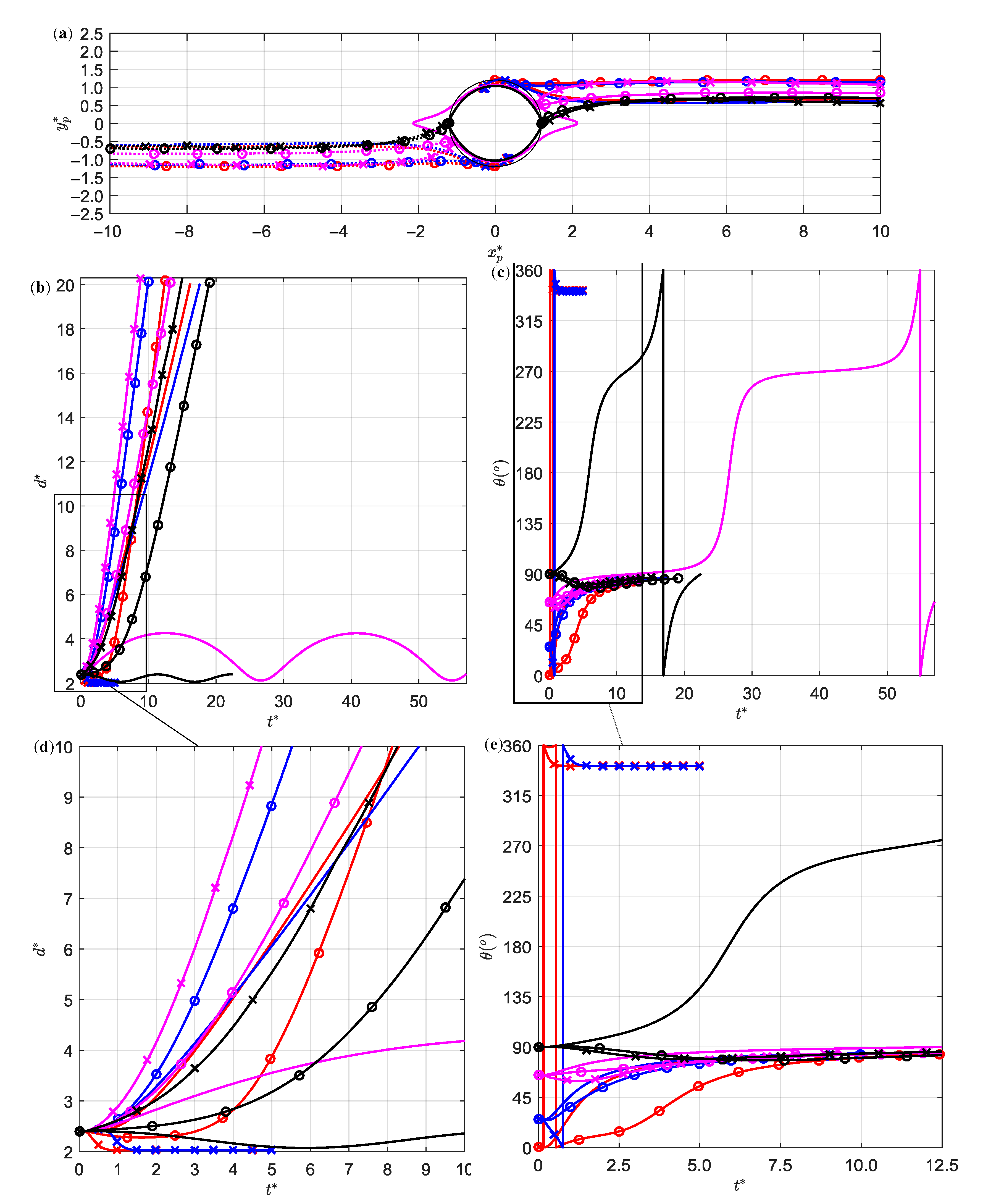
Finally, the particle dynamics were observed at their closest initial distance $d_0^{*}=2.4$, as seen in Figure 8. In Figure 8a,b, the magnetic force was stronger than the viscous force for the initial particle orientations ${\theta }_0=0^{\circ }$ and ${\theta }_0={25}^{\circ }$ at $H_0=5000$ A/m, and ${\theta }_0=0^{\circ }$, ${\theta }_0={25}^{\circ }$, and ${\theta }_0={65}^{\circ }$ at $H_0=$ 10,000 A/m. In these cases, the particle distances monotonically decreased until a chain was formed at ${\theta }^{RL,ss}$, as seen in Figure 8c,e. At all other initial orientations, however, the viscous force was stronger than the magnetic force, and thus, the particle distances increased at different rates, except at ${\theta }_0={65}^{\circ }$ and ${\theta }_0={90}^{\circ }$, in the absence of a magnetic field. At a magnetic field strength $H_0=$ 10,000 A/m, the particles separated faster at ${\theta }_0={65}^{\circ }$ than all other magnetic field strengths and orientations. For the magnetic field strength $H_0=5000$ A/m, the particle orientation ${\theta }_0={65}^{\circ }$ had a faster separation rate than at ${\theta }_0={90}^{\circ }$. In fact, initially, the particle separation rate for $H_0=5000$ A/m and ${\theta }_0={65}^{\circ }$ was slower because the particle orientation rotated backwards, as seen in Figure 8c,e, before monotonically increasing. Similar to other distances, however, the initial particle orientation of ${\theta }_0={90}^{\circ }$ monotonically decreased and then increased. The rates of the orientation decreasing and/or increasing, the rate of the periodic orientation, or if a chain is being formed depended on the particles’ positions in the fluid domain and the initial orientations. The further away the particles were from the origin, the faster the separation rate and, consequentially, the faster the particle orientation approached $\theta ={90}^{\circ }$.

As observed for the RL-configuration, it was more feasible for the particles to form a chain under a uniform magnetic field, including the strengths $H_0=5000$ A/m and $10,000$ A/m. Similar to the LR-configuration, the particles repelled at ${\theta }_0={90}^{\circ }$. In a couple of cases, the magnetic force was initially greater than the viscous force, and the particle orientation rotated backwards at the same time that they were attracting each other, but the viscous force eventually broke the attraction.

4.3. Comparison between Configurations

We conclude the analysis by comparing the LR- and RL-configurations. At the initial distance $d_0^{*}=4$, the particles separated at different rates because the viscous force was larger, and the particles repelled each other when their orientations were above their respective critical values. As the initial particle distance decreased, the magnetic force became more significant than the viscous force. The particles in the LR-configuration were more susceptible to forming a staggered chain than the RL-configuration, and their stable steady orientations ${\theta }^{LR,ss}$ and ${\theta }^{RL,ss}$ are shown in Table 1 and Table 2, respectively. Additionally, whether or not the particles formed a chain under a magnetic field, the particles’ directions were always pinned at stable steady angles where ${\varphi }_1^{ss,LR}\approx {\varphi }_2^{ss,RL}$ and ${\varphi }_2^{ss,LR}\approx {\varphi }_1^{ss,RL}$ because the magnetic torque was greater than the hydrodynamic torque.

5. Conclusions

We conducted a numerical investigation based on the dynamics of two magnetic Janus particles under a uniform magnetic field and in a simple shear flow by DNS using an FEM model and applying the ALE method. Depending on the particle configurations, their dynamics were affected by their initial distances, their initial orientation, and the magnetic field strength. For the largest initial distance, both particles might initially attract each other in some cases, but will nonetheless separate due to the increased strength of the viscous force, and consequentially, the particle orientation would increase. Over time, as the particle orientation became greater than the configurations’ respective critical values, the particles would repel each other, thus increasing the separation rate when combined with the hydrodynamic separation from the shear flow. For initial orientations greater than the critical orientation, the particles repelled each other, and their separation increased. Additionally, at ${\theta }_0={90}^{\circ }$, the particles would break the periodic orbiting cycle, as opposed to when they were under a simple shear flow in the absence of a magnetic field. For some configurations experiencing the same magnetic field strength, the Janus particles would either attract or separate faster than the other configuration due to their different critical orientations. Since the shear rate was low, however, the Janus particles’ direction would be pinned at a stable steady angle, and ${\varphi }_1^{ss,LR}\approx {\varphi }_2^{ss,RL}$ and ${\varphi }_1^{ss,RL}\approx {\varphi }_2^{ss,LR}$.

As the initial particle distance decreased, the magnetic force increased due to the lower viscous force near the origin. Therefore, a particle chain became more feasible for both configurations at a stable steady orientation. For the LR-configuration and the magnetic field strength of $H_0=5000$ A/m, the particles would still separate. On the other hand, for the RL-configuration, a chain formation was possible under moderate and strong magnetic regimes. When their initial orientations were above their respected critical values, the particles repelled each other and separated under the shear flow, except for one case under the RL-configuration.

For future research involving magnetic Janus particles, the following could be considered:

• Arbitrary initial particle directions.
• Adding more than two particles in a simple shear flow and under a uniform magnetic field.
• Studying how a chain or flail of particles can break up under a simple shear flow.
• Investigating different magnetic susceptibilities where one side is non-magnetic and the other side has a different magnetic susceptibility ($\chi \ne 1$), when both sides are magnetic and have different susceptibilities, and where two or more particles have different susceptibilities.
• Placing two particles in a Poiseuille and/or in a Couette flow.
• Examining at least two particles with arbitrary sizes.

Overall, in future research studies, the Mason number would be significant to study chain formation for two-dimensional studies, a three-dimensional structure formation, or ruptures in fluid flows. Certainly, a very desirable research outcome would include theoretical or approximate equations for two Janus particles under a uniform magnetic field without a simple shear flow, and under a uniform magnetic field with a simple shear flow. Fortunately, there are many research articles that have ventured into two solid magnetic particles in a simple shear flow and/or under a uniform magnetic field. Therefore, a possible study to consider is for future authors to compare the behaviors of two anisotropic particles with two isotropic particles and analyze the angular velocities, their distance separation and attraction rates, the critical particle orientation, and chain formations. If there existed more than two Janus particles, newer structures could be fabricated by anisotropic particles as a new approach for applications in valves, breaks, dampers, etc. Furthermore, because the configurations are an additional variable (along with orientation, distance, and, possibly, particle direction), more investigations are needed to carefully evaluate chains and clusters under fluid flow, along with a careful numerical design and experiment on the observation and control of magnetic Janus particles. One way to analyze Janus particles is to evaluate how staggered chains and clusters, with relative configurations and stable steady orientations, can possibly affect the viscosity of the magnetorheological fluids, how they rearrange themselves in low and high fluid velocities, create complex branches under high magnetic fields, or rupture under high fluid velocities. Although we only focused on a pair of Janus particles, we would like to stress that future numerical applications should include a moderate amount of particles to analyze cluster or chain formation in fluid flows similar to how Seong et al. and Kim et al. validated their model with past experimental applications. This research and other future research articles can assist with the study and development of smart fluids that contain anisotropic particles, for many applications in industrial and biomedical sciences.

References

- De Gennes, P.G. Soft matter. Rev. Mod. Phys. 1992, 64, 645. [Google Scholar] [CrossRef]
- Perro, A.; Reculusa, S.; Ravaine, S.; Bourgeat-Lami, E.; Duguet, E. Design and synthesis of Janus micro-and nanoparticles. J. Mater. Chem. 2005, 15, 3745–3760. [Google Scholar] [CrossRef]
- Su, H.; Price, C.A.H.; Jing, L.; Tian, Q.; Liu, J.; Qian, K. Janus particles: Design, preparation, and biomedical applications. Mater. Today Bio. 2019, 4, 100033. [Google Scholar] [CrossRef] [PubMed]
- Ruditskiy, A.; Ren, B.; Kretzschmar, I. Behaviour of iron oxide (Fe3O4) Janus particles in overlapping external AC electric and static magnetic fields. Soft Matter 2013, 9, 9174–9181. [Google Scholar] [CrossRef]
- Yu, S.; Ma, N.; Yu, H.; Sun, H.; Chang, X.; Wu, Z.; Deng, J.; Zhao, S.; Wang, W.; Zhang, G.; et al. Self-Propelled Janus Microdimer Swimmers under a Rotating Magnetic Field. Nanomaterials 2019, 9, 1672. [Google Scholar] [CrossRef] [Green Version]
- Lee, S.Y.; Yang, S. Compartment fabrication of magneto-responsive Janus microrod particles. Chem. Commun. 2015, 51, 1639–1642. [Google Scholar] [CrossRef] [PubMed]
- Yuet, K.P.; Hwang, D.K.; Haghgooie, R.; Doyle, P.S. Multifunctional superparamagnetic Janus particles. Langmuir 2010, 26, 4281–4287. [Google Scholar] [CrossRef]
- Hu, J.; Zhou, S.; Sun, Y.; Fang, X.; Wu, L. Fabrication, properties and applications of Janus particles. Chem. Soc. Rev. 2012, 41, 4356–4378. [Google Scholar] [CrossRef]
- Varma, V.B.; Wu, R.G.; Wang, Z.P.; Ramanujan, R.V. Magnetic Janus particles synthesized using droplet micro-magnetofluidic techniques for protein detection. R. Soc. Chem. 2017, 17, 3514–3525. [Google Scholar] [CrossRef]
- Yang, S.M.; Kim, S.H.; Lim, J.M.; Yi, G.R. Synthesis and assembly of structured colloidal particles. J. Mater. Chem. 2008, 18, 2177–2190. [Google Scholar] [CrossRef]
- Ashtiani, M.; Hashemabadi, S.H.; Ghaffari, A. A review on the magnetorheological fluid preparation and stabilization. J. Magn. Magn. Mater. 2015, 374, 716–730. [Google Scholar] [CrossRef]
- Campuzano, S.; Gamella, M.; Serafín, V.; Pedrero, M.; Yáñez-Sedeño, P.; Pingarrón, J.M. Magnetic Janus particles for static and dynamic (bio) sensing. Magnetochemistry 2019, 5, 47. [Google Scholar] [CrossRef] [Green Version]
- Moran, J.L.; Posner, J.D. Phoretic self-propulsion. Annu. Rev. Fluid Mech. 2017, 7, 511–540. [Google Scholar] [CrossRef]
- Yan, J.; Bae, S.C.; Granick, S. Colloidal superstructures programmed into magnetic Janus particles. Adv. Mater. 2015, 27, 874–879. [Google Scholar] [CrossRef]
- Li, W.; Dong, H.; Tang, G.; Ma, T.; Cao, X. Controllable microfluidic fabrication of Janus and microcapsule particles for drug delivery applications. RSC Adv. 2015, 5, 23181–23188. [Google Scholar] [CrossRef]
- Kaewsaneha, C.; Bitar, A.; Tangboriboonrat, P.; Polpanich, D.; Elaissari, A. Fluorescent-magnetic Janus particles prepared via seed emulsion polymerization. J. Colloid Interface Sci. 2014, 424, 98–103. [Google Scholar] [CrossRef]
- Zhao, R.; Han, T.; Sun, D.; Huang, L.; Liang, F.; Liu, Z. Poly (ionic liquid)-modified magnetic Janus particles for dye degradation. Langmuir 2019, 35, 11435–11442. [Google Scholar] [CrossRef]
- Smoukov, S.K.; Gangwal, S.; Marquez, M.; Velev, O.D. Reconfigurable responsive structures assembled from magnetic Janus particles. Soft Matter 2009, 5, 1285–1292. [Google Scholar] [CrossRef]
- Kang, T.G.; Hulsen, M.A.; den Toonder, J.M.; Anderson, P.D.; Meijer, H.E. A direct simulation method for flows with suspended paramagnetic particles. J. Comput. Phys. 2008, 227, 4441–4458. [Google Scholar] [CrossRef]
- Zhang, J.; Zhou, R.; Wang, C. Dynamics of a pair of ellipsoidal microparticles under a uniform magnetic field. J. Micromech. Microeng. 2019, 29, 104000. [Google Scholar] [CrossRef]
- Ren, B.; Ruditskiy, A.; Song, J.H.; Kretzschmar, I. Assembly behavior of iron oxide-capped Janus particles in a magnetic field. Langmuir 2012, 28, 1149–1156. [Google Scholar] [CrossRef] [PubMed]
- Ren, B.; Kretzschmar, I. Viscosity-dependent Janus particle chain dynamics. Langmuir 2013, 29, 14779–14786. [Google Scholar] [CrossRef] [PubMed]
- Long, T.W.; Cordova-Figueroa, U.M.; Kretzschmar, I. Measuring, modeling, and predicting the magnetic assembly rate of 2D-staggered janus particle chains. Langmuir 2019, 35, 8121–8130. [Google Scholar] [CrossRef]
- Steinbach, G.; Nissen, D.; Albrecht, M.; Novak, E.V.; Sánchez, P.A.; Kantorovich, S.S.; Gemming, S.; Erbe, A. Bistable self-assembly in homogeneous colloidal systems for flexible modular architectures. Soft Matter 2016, 12, 2737–2743. [Google Scholar] [CrossRef] [PubMed] [Green Version]
- Darabaner, C.L.; Raasch, J.K.; Mason, S.G. Particle motions in sheared suspensions XX: Circular cylinders. Can. J. Chem. Eng. 1967, 45, 3–12. [Google Scholar] [CrossRef]
- Bartok, W.; Mason, S.G. Particle motions in sheared suspensions: V. Rigid rods and collision doublets of spheres. J. Colloid Sci. 1957, 12, 243–262. [Google Scholar] [CrossRef]
- Darabaner, C.L.; Mason, S.G. Particle motions in sheared suspensions XXII: Interactions of rigid spheres (experimental). Rheol. Acta 1967, 6, 273–284. [Google Scholar] [CrossRef]
- Wakiya, S.; Darabaner, C.L.; Mason, S.G. Particle motions in sheared suspensions XXI: Interactions of rigid spheres (theoretical). Rheol. Acta 1967, 6, 264–273. [Google Scholar] [CrossRef]
- Arp, P.A.; Mason, S.G. The kinetics of flowing dispersions: VIII. Doublets of rigid spheres (theoretical). J. Colloid Interface Sci. 1977, 61, 21–43. [Google Scholar] [CrossRef]
- Van de Ven, T.G.M.; Mason, S.G. The microrheology of colloidal dispersions: IV. Pairs of interacting spheres in shear flow. J. Colloid Interface Sci. 1976, 57, 505–516. [Google Scholar] [CrossRef]
- Lin, C.J.; Lee, K.J.; Sather, N.F. Slow motion of two spheres in a shear field. J. Fluid Mech. 1970, 43, 35–47. [Google Scholar] [CrossRef]
- Van de Ven, T.G.M.; Mason, S.G. The microrheology of colloidal dispersions: V. Primary and secondary doublets of spheres in shear flow. J. Colloid Interface Sci. 1976, 57, 517–534. [Google Scholar] [CrossRef]
- Kang, T.G.; Hulsen, M.A.; den Toonder, J.M. Dynamics of magnetic chains in a shear flow under the influence of a uniform magnetic field. Phys. Fluids 2012, 24, 042001. [Google Scholar] [CrossRef] [Green Version]
- Rosenfeld, N.C.; Wereley, N.M. Volume-constrained optimization of magnetorheological and electrorheological valves and dampers. Smart Mater. Struct. 2004, 13, 1303. [Google Scholar] [CrossRef]
- Oh, J.-S.; Shul, C.W.; Kim, T.H.; Lee, T.-H.; Son, S.-W.; Choi, S.-B. Dynamic Analysis of Sphere-Like Iron Particles Based Magnetorheological Damper for Waveform-Generating Test System. Int. J. Mol. Sci. 2020, 21, 1149. [Google Scholar] [CrossRef] [Green Version]
- Anupama, A.V.; Kumaran, V.; Sahoo, B. Application of monodisperse Fe3O4 submicrospheres in magnetorheological fluids. J. Ind. Eng. Chem. 2018, 67, 347–357. [Google Scholar] [CrossRef]
- Seong, Y.; Kang, T.G.; Hulsen, M.A.; den Toonder, J.M.; Anderson, P.D. Magnetic interaction of Janus magnetic particles suspended in a viscous fluid. Phys. Rev. E 2016, 93, 022607. [Google Scholar] [CrossRef] [Green Version]
- Kim, H.E.; Kang, T.G. Direct Simulation of the Magnetic Interaction of Elliptic Janus Particles Suspended in a Viscous Fluid. Trans. Korean Soc. Mech. Eng. B 2017, 41, 455–462. [Google Scholar]
- Kim, H.E.; Kim, K.; Ma, T.Y.; Kang, T.G. Numerical investigation of the dynamics of Janus magnetic particles in a rotating magnetic fiel. Korea Aust. Rheol. J. 2017, 29, 17–27. [Google Scholar] [CrossRef]
- Zhang, J.; Sobecki, C.; Wang, C. Numerical investigation of dynamics of elliptical magnetic microparticles in shear flow. Microfluid. Nanofluidic 2018, 22, 83. [Google Scholar] [CrossRef]
- Zhang, J.; Wang, C. Numerical study of lateral migration of elliptical magnetic microparticles in microchannels in uniform magnetic fields. Magnetochemistry 2018, 4, 16. [Google Scholar] [CrossRef] [Green Version]
- Sobecki, C.; Zhang, J.; Wang, C. Numerical Study of Paramagnetic Elliptical Microparticles in Curved Channels and Uniform Magnetic Fields. Micromachines 2020, 11, 37. [Google Scholar] [CrossRef]
- Cao, Q.; Li, Z.; Wang, Z.; Han, X. Rotational motion and lateral migration of an elliptical magnetic particle in a microchannel under a uniform magnetic field. Microfluid. Nanofluidics 2018, 22, 3. [Google Scholar] [CrossRef]
- Zhou, R.; Sobecki, C.A.; Zhang, J.; Zhang, Y.; Wang, C. Magnetic control of lateral migration of ellipsoidal microparticles in microscale flows. Phys. Rev. Appl. 2017, 8, 024019. [Google Scholar] [CrossRef]
- Arp, P.A.; Mason, S.G. Particle behavior in shear and electric fields. VIII. Interactions of pairs of conducting spheres (theoretical). Colloid Polym. Sci. 1977, 255, 566–584. [Google Scholar] [CrossRef]
Figure 1.
(a) Schematic of two Janus particles in a simple shear flow and under a uniform magnetic field. The particles are in a fluid domain , and the magnetic field is produced inside the air domain . The particle angles are shown in the LR-configuration box (b), and the orientation and the center-to-center distances are seen in the RL-configuration box (c). The initial orientation used in this study are either equal to or in between (d) and (e) .
Figure 2.
Validation and path of (a) two Janus particles in a simple shear flow in the absence of a magnetic field with an initial distance of . The direction and dimensionless angular velocity, with respect to dimensionless time, for (b) a single Janus particle rotating in a magnetic field without a simple shear flow and the motions of two Janus particles in the (c) LR- and (d) RL-configurations in a magnetic field without a simple shear flow and with an initial distance of . The particles in (a) show that Particles 1 (dotted line and star at the initial orientation) and 2 (solid line and circle at the initial orientation) separate at (red lines), but orbit each other at (black lines). A single Janus particle in (b) has an initial direction at . The angular velocity is at its maximum at and at its minimum at and . In (c), the attraction and the repulsion-attraction for both Janus particles at their initial orientations (red), (blue), and (black) for the LR-configuration. Similar results are shown in (d) with initial orientations (red), (blue), and (black). The symbols shown are data points from the authors’ results for comparison to the simulation results. The critical orientations for LR- and RL-configurations are and , respectively.
Figure 3.
Numerical results for the LR-configuration at . We see the results for (a) the center of mass position for Particle 1 (dotted-line) and Particle 2 (solid line), (b) the distance between two particles over time, and (c) the particle orientation over time. The particles were observed for the initial orientations (red), (blue), (magenta), and (black) under the magnetic field strengths A/m (no symbol), A/m (circle), and 10,000 A/m (cross). The particle dynamics in (d) and (e) are the enlarged graphs for (b) and (c), respectively.
Figure 4.
Figure 5.
Figure 6.
Numerical results for the RL-configuration at . We see the results for (a) the center of mass position for Particle 1 (dotted-line) and Particle 2 (solid line), (b) the distance between two particles over time, and (c) the particle orientation over time. The particles were observed for the initial orientations (red), (blue), (magenta), and (black) under the magnetic field strengths A/m (no symbol), A/m (circle), and 10,000 A/m (cross). The particle dynamics in (d) and (e) are the enlarged graphs for (b) and (c), respectively.
Figure 7.
Figure 8.