Impact of Uncertainty in the Input Variables and Model Parameters on Predictions of a Long Short Term Memory (LSTM) Based Sales Forecasting Model

Abstract

A Long Short Term Memory (LSTM) based sales model has been developed to forecast the global sales of hotel business of Travel Boutique Online Holidays (TBO Holidays). The LSTM model is a multivariate model; input to the model includes several independent variables in addition to a dependent variable, viz., sales from the previous step. One of the input variables, “number of active bookers per day”, is estimated for the same day as sales. This need for estimation requires the development of another LSTM model to predict the number of active bookers per day. The number of active bookers is variable, so the predicted is used as an input to the sales forecasting model. The use of a predicted variable as an input variable to another model increases the chance of uncertainty entering the system. This paper discusses the quantum of variability observed in sales predictions for various uncertainties or noise due to the estimation of the number of active bookers. For the purposes of this study, different noise distributions such as normalized, uniform, and logistic distributions are used, among others. Analyses of predictions demonstrate that the addition of uncertainty to the number of active bookers via dropouts as well as to the lagged sales variables leads to model predictions that are close to the observations. The least squared error between observations and predictions is higher for uncertainties modeled using other distributions (without dropouts) with the worst predictions being for Gumbel noise distribution. Gaussian noise added directly to the weights matrix yields the best results (minimum prediction errors). One possibility of this uncertainty could be that the global minimum of the least squared objective function with respect to the model weight matrix is not reached, and therefore, model parameters are not optimal. The two LSTM models used in series are also used to study the impact of corona virus on global sales. By introducing a new variable called the corona virus impact variable, the LSTM models can predict corona-affected sales within five percent (5%) of the actuals. The research discussed in the paper finds LSTM models to be effective tools that can be used in the travel industry as they are able to successfully model the trends in sales. These tools can be reliably used to simulate various hypothetical scenarios also.

1. Introduction

Traditionally, various techniques such as Autoregression (AR) [1,2], Moving Average (MA) [3,4], Exponential Smoothing (ES) [5], Hybrid Methods (HM) [6,7,8], and Autoregressive Integrated Moving Average (ARIMA) [9] have been used to predict and forecast the dependent variable in a time series [1,2,3,4,5,6,7,8,9]. These techniques have recently been used in conjunction with artificial neural network algorithms. Among these techniques, the ARIMA model has mostly outperformed others in precision and accuracy [10].

With the recent advancement in computational power and more importantly the development of more advanced machine learning techniques such as deep learning, new algorithms have been developed to analyse and forecast time series data. Research [11,12] showed that newly developed deep learning-based algorithms for forecasting time series data such as “Long Short-Term Memory (LSTM)” are superior to traditional algorithms such as ARIMA models.

Recurrent neural networks with Long Short-Term Memory [13] (which are concisely referred to as LSTMs) have emerged as effective and scalable models for several learning problems related to sequential data. Earlier methods of forecasting time series data have either been tailored towards a specific problem or did not scale to extended time dependencies. Scaling for seasonality is a challenge in non-LSTM models requiring manual feature extraction [14,15]. LSTMs, on the other hand, are both general in nature and effective at capturing long-term temporal dependencies. They are good at extracting the patterns in the input feature space and handling the nonlinear and complex feature interactions in the data without explicitly defining them. This makes LSTM models highly scalable but more complex than the other time series models. As the name suggests, LSTMs memorize the happenings of the distant past and the near past and balance out the two when making predictions resulting in augmented accuracy.

One central challenge in any modeling exercise is understanding and handling the uncertainty embedded in the model input (dependent variables) and that in the model parameters (constants). Model constants are determined by fitting the model output to the observations in such a way that the error in predictions is minimized, most often, in the least square sense. The model constants in such a case are considered to be deterministic, as a given model constant has one and only one value instead of a spread with a mean and a standard deviation. Such deterministic models predict one and only one value of the output variable for a given set of input variables. A stochastic model, on the other hand, has uncertainty built into the input variables and the model constants. As a result, instead of predicting only a single value of the dependent variable, stochastic models predict a spread in the dependent variable.

Businesses face various type of uncertainties for a number of reasons that could be related to operational challenges, finances, technology, and nature. This uncertainty also finds its way in the forecasting model in the form of random noise associated with input data and the residual error in the model training. Analysis of uncertainty is performed to understand [16,17] when the model predictions are underconfident and when they are overconfident. This analysis is performed by quantifying prediction intervals [18,19] and applying these predictions in decision making.

The uncertainties in predictions can be described in a probabilistic framework [20], which has a central role in machine learning models. Statistics provides us with a way [21] to present the data not as measurements but as estimates with error (uncertainties). Uncertainty in models also affects the model selection process [22] and plays a role in hyperparameter optimization. In this study, we used dropouts in the neural network layers and introduced random noise in both the inputs and model weights to measure uncertainty. We discussed how dropouts in the neural network are more effective in measuring uncertainty without compromising model accuracy and complexity.

This paper summarizes the results of research performed to understand how uncertainty impacts predictions and compares the performance of deterministic and stochastic models. Furthermore, the study also investigates the impact of uncertainty in input variables versus uncertainty in model constants on the prediction accuracy of the dependent variable. Different mathematical distributions for uncertainties were modeled. LSTM models are used to predict sales forecasts for a complete month and uncertainty analyses are performed with respect to the same. A brief description of the LSTM model architecture is provided in the next section.

2. Theoretical Foundations

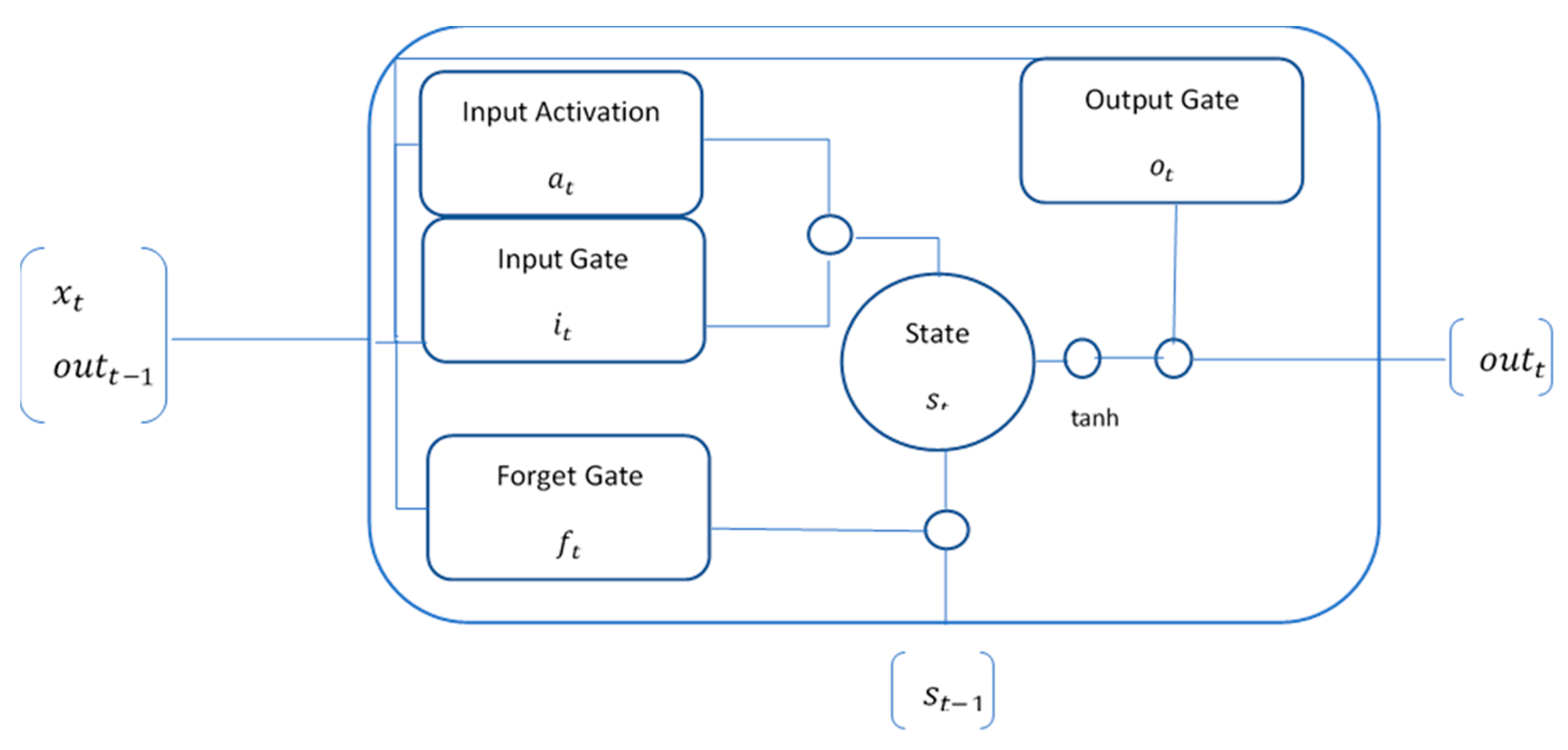
LSTM Architecture

The central idea behind the LSTM architecture [23] is a memory cell, which can maintain its state over time, and nonlinear gating units, which regulate the information flow into and out of the cell. A common LSTM unit is composed of a cell, an input gate, an output gate, and a forget gate. A schematic of a simple LSTM block can be seen in Figure 1. The cell remembers values over arbitrary time intervals, and the three gates regulate the flow of information into and out of the cell.

Input gate determines the new data that get stored in the cell through a sigmoid layer followed by a tanh layer. The initial sigmoid layer, called the “input door layer”, identifies the values that will be modified. Next, a tanh layer makes a vector of new candidate values that could be added to the state.

The forget gate decides on the information that needs to be discarded from the cell state using a sigmoid layer that outputs a number between 0 and 1, where 1 means “completely keep this”, and 0 implies “completely ignore this”.

Output gate determines the information (yield) that goes out of each cell. The yielded value will be based on the cell state along with the filtered and newly added data.

Let $x_t\in {ℛ}^M$ be the input vector at time t, T be the number of LSTM blocks, and M be the number of inputs. Then, we get the following weights for an LSTM layer:

Input weights: $W_{xs}, W_{xi}, W_{xf}, W_{xo}\in {ℛ}^{T\times M}$ for activation, input, forget, and output gate, respectively.

Recurrent weights: $W_{hs}, W_{hi}, W_{hf}, W_{ho}\in {ℛ}^{T\times T}$ for activation, input, forget, and output gate, respectively.

Bias weights: $b_s, b_i, b_f, b_o \in {ℛ}^T$ for activation, input, forget, and output gate, respectively.

Symbols of matrix products:

• $\odot$: Represents the elementwise product or Hadamard product.
• $\otimes$: Represents the outer product.
• $·$: Represents the inner product.

The gates are defined as:

Input activation:	$a_t=\tanh \left(W_{xs}·x_t + W_{hs}·ou{t}_{t-1}+ b_s\right);$	(1)
Input gate:	$i_t=\mathsf{\sigma }\left(W_{xs}·x_t + W_{hs}·ou{t}_{t-1}+ b_s\right);$	(2)
Forget gate:	$f_t=\mathsf{\sigma }\left(W_{xf}·x_t + W_{hf}·ou{t}_{t-1}+ b_f\right);$	(3)
Output gate:	$o_t=\mathsf{\sigma }\left(W_{xo}·x_t + W_{ho}·ou{t}_{t-1}+ b_o\right);$	(4)
Internal state:	$s_t=a_t\odot i_t+ f_t\odot s_{t-1};$	(5)
Output	$ou{t}_t=\tanh \left(s_t\right)\odot o_t.$	(6)

Backpropagation:

The deltas inside the LSTM block are then calculated as

$$d{o}_t = \tanh \left(s_t\right)dou{t}_t$$

$$d{s}_t = (1-tan{h}^2\left(s_t\right))dou{t}_t$$

$$d{f}_t = s_{t-1}d{s}_t$$

$$d{s}_{t-1} = d{s}_t+ f_{t}d{s}_t$$

$$d{i}_t= a_{t}d{s}_t$$

$$d{a}_t = i_{t}d{s}_t$$

The updates in the weights can be formulated as

$$d{W}_{xo}={{\displaystyle \sum }}_t{o}_t\left(1-o_t\right)x_{t}d{o}_t$$

$$d{W}_{xi}={{\displaystyle \sum }}_t{i}_t\left(1-i_t\right)x_{t}d{i}_t$$

$$d{W}_{xf}={{\displaystyle \sum }}_{t}f\left(1-f_t\right)x_{t}d{f}_t$$

$$d{W}_{xs}={{\displaystyle \sum }}_t\left(1-a_t^2\right)x_{t}d{a}_t$$

And,

$$d{W}_{ho}={{\displaystyle \sum }}_t{o}_t\left(1-o_t\right)h_{t-1}d{o}_t$$

$$d{W}_{hi}={{\displaystyle \sum }}_t{i}_t\left(1-i_t\right)h_{t-1}d{i}_t$$

$$d{W}_{hf}={{\displaystyle \sum }}_{t}f\left(1-f_t\right)h_{t-1}d{f}_t$$

$$d{W}_{hs}={{\displaystyle \sum }}_t\left(1-a_t^2\right)h_{t-1}d{a}_t$$

$$d{h}_{t-1}= o_t\left(1-o_t\right)W_{ho}d{o}_t+ i_t\left(1-i_t\right)W_{hi}d{i}_t+f_t\left(1-f_t\right)W_{hf}d{f}_t+ \left(1-a_t^2\right)W_{hc}d{a}_t$$

Having understood the mathematical formulation of an LSTM model, the next step is to discuss the approach taken to model the sales forecasting using the LSTM algorithm.

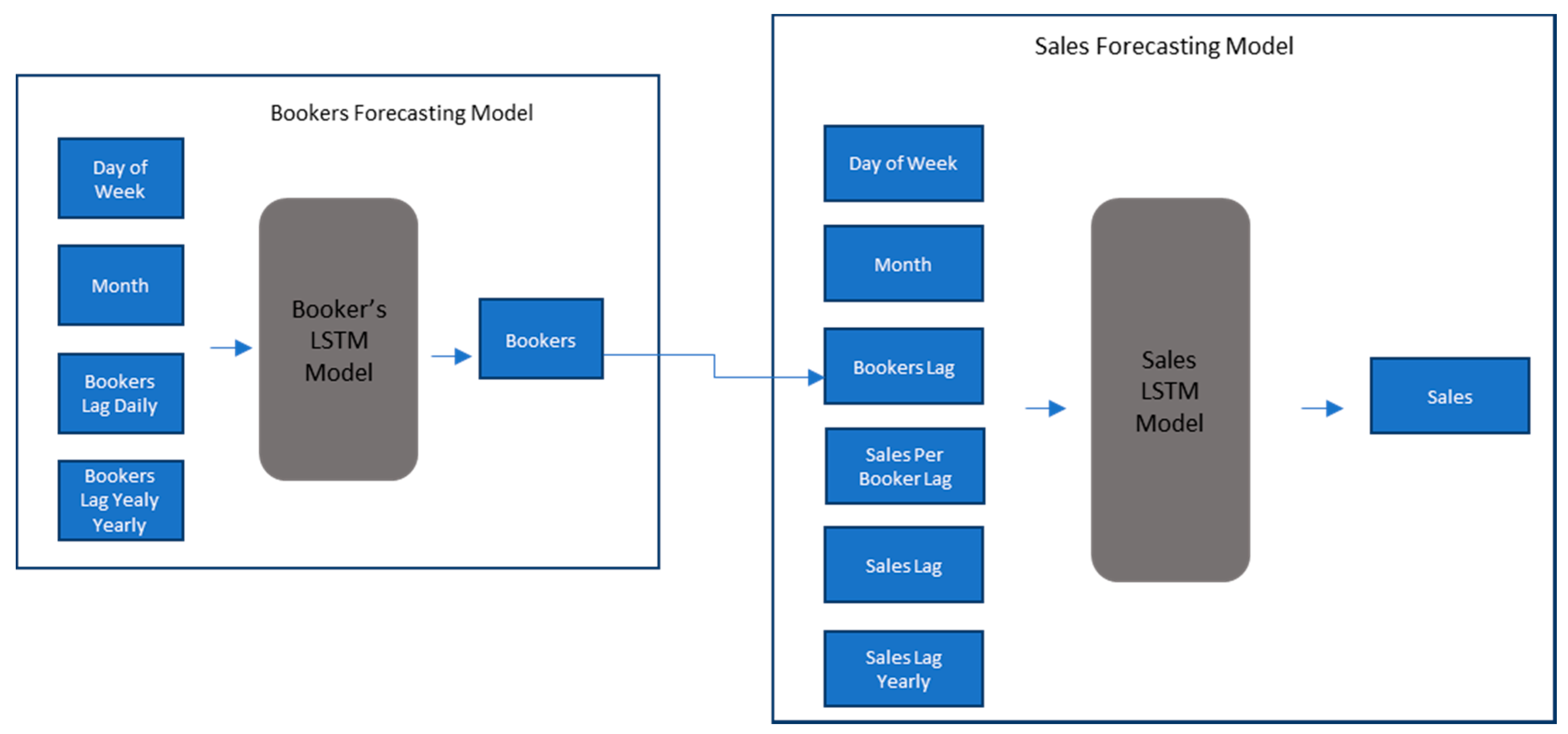
3. Materials and Methods

In this section, we present the approach to modeling sales forecasts. The sales forecasting model has two underlying LSTM models, as shown in Figure 2. The first model predicts the number of active bookers on a given day, and the prediction is based on the daily lag of active bookers, yearly lag of active bookers, day of the week, and month of the year variables. The output of the bookers model was used as an input in the second LSTM model, which forecasted the global sales. The sales forecasting model had the inputs such as sales from the previous step, yearly lag of sales (accounts for the seasonality), day of the week, month of the year, active bookers count, and sales per active booker. Each sequence of dataset fed into an LSTM cell that consisted of the previous seven (7) days of data. Both the models made predictions one time step [24] at a time, and these predictions were used as inputs to make predictions at the next time step. Both the models (active booker count and sales forecast) have two LSTM layers of 100 neurons each, followed by an output dense layer with one neuron.

To model uncertainty in a neural network model, there could be several approaches e.g., Monte Carlo [25] simulation, Bayesian Neural Network [26], and use of Dropouts in between the LSTM layers. A study conducted by Yarin Gal and Zoubin Ghahramani [16] showed how uncertainty can be modeled with dropouts in Neural Networks to improve the performance of log-likelihood and RMSE compared to existing state-of-the-art methods. In deep neural networks, dropout is a technique that is used to avoid overfitting.

Figure 3 shows a high-level pictorial representation of the three components of the model where uncertainties could lie.

For the purposes of this study, the predictions were made and compared with actual observations using the above models (Figure 2) and the following approaches (cases).

Case 1: Deterministic approach: In this approach, dropouts are not used at the time of predictions.

Case 2: Stochastic dropout approach: In this approach, dropouts [27] are used at both training and prediction stages. Three combination of models are run for stochastic dropout approach, viz.

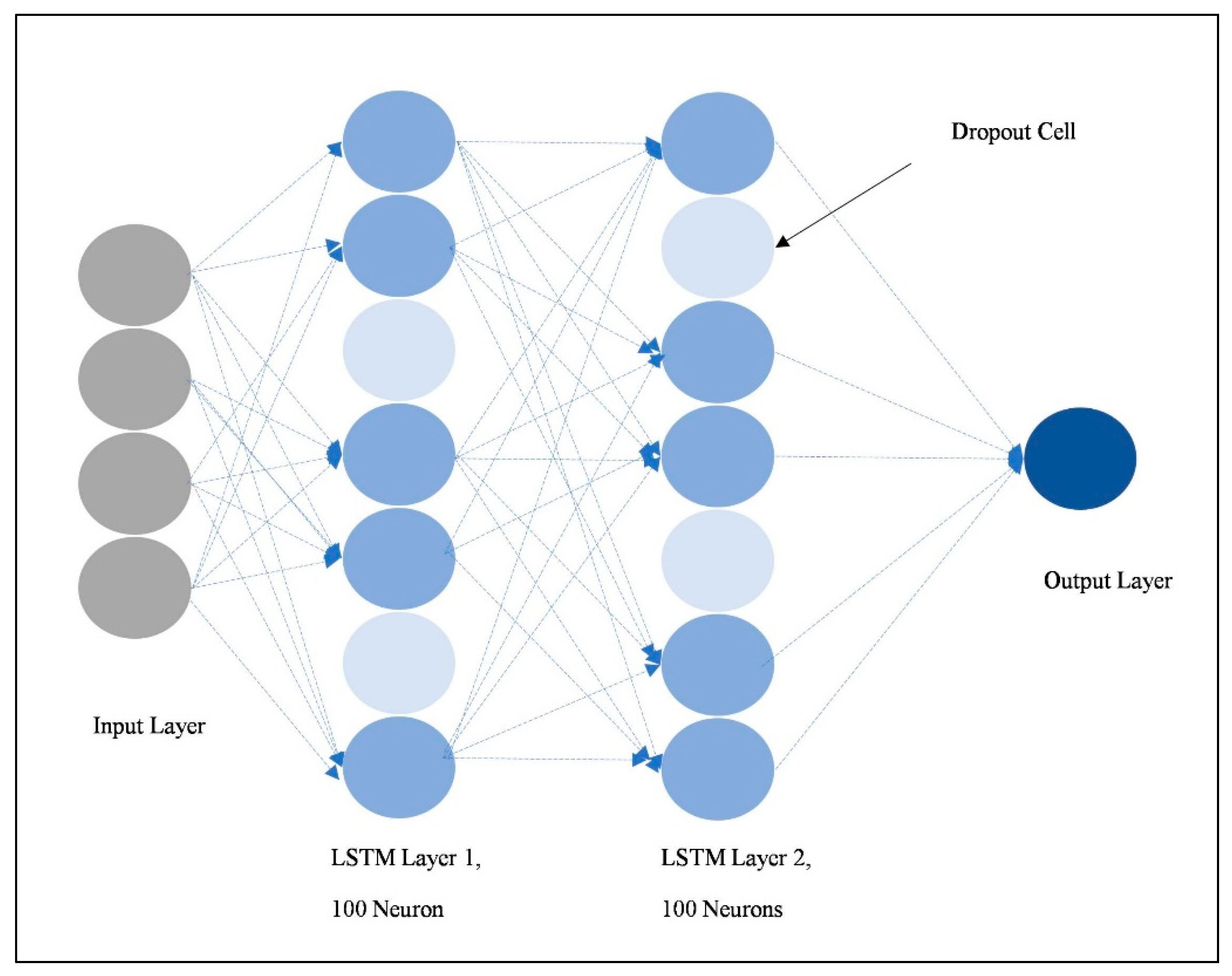
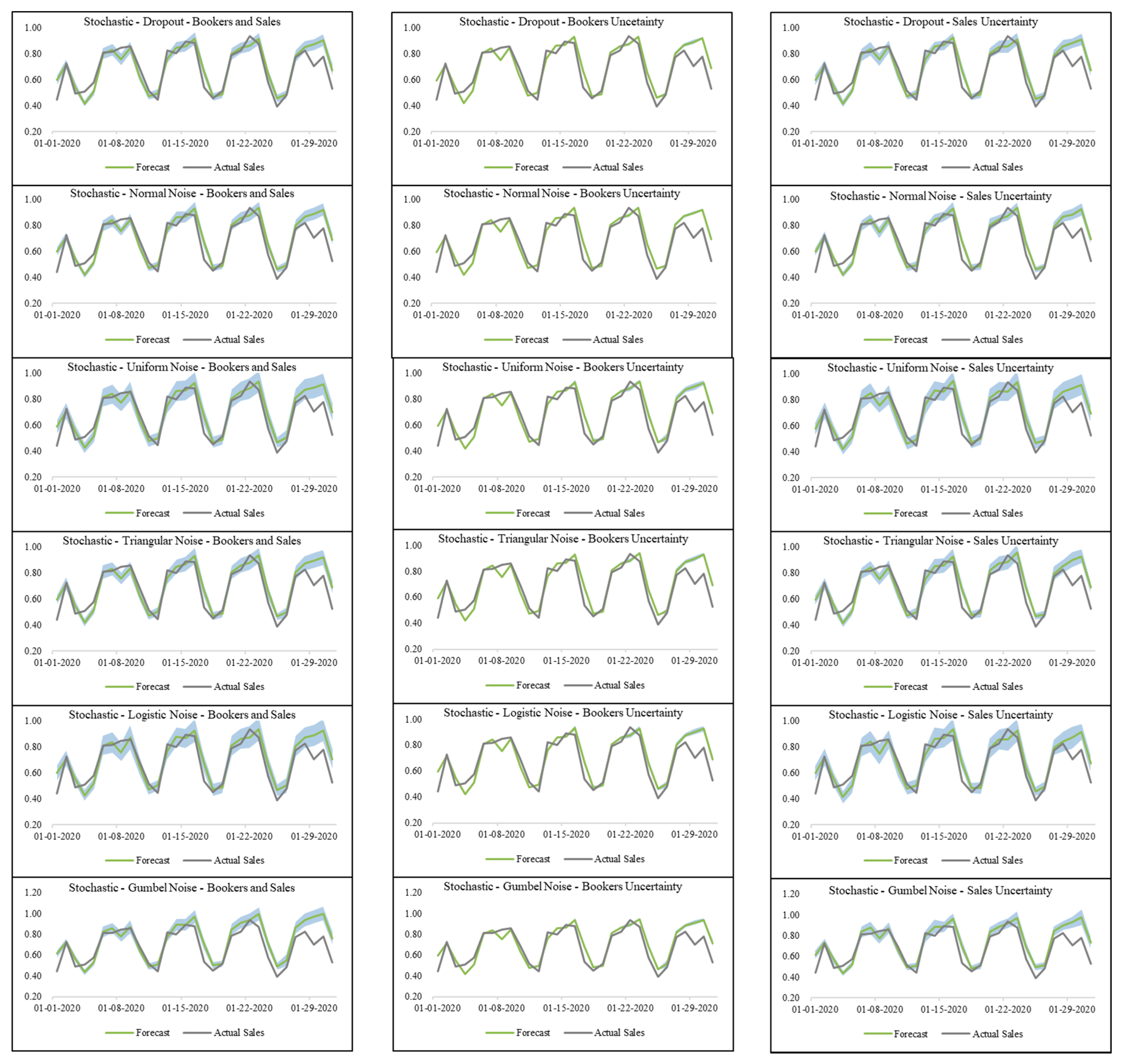
• The dropouts are only used in the active booker count model and not in the sales model at the time of prediction,
• The dropouts are only used in the sales model and not in the active booker count model at the time of prediction,
• The dropouts are used in both the sales and the active booker count models at the time of prediction.

A recurrent dropout with a dropout rate of 20% and a kernel dropout with dropout rate of 10% in the LSTM layers were used. Figure 4 shows a schematic representation of dropouts in neural network layers.

Case 3: Stochastic noise in predicted active booker count and sales: In this approach, instead of using dropouts at the time of prediction, various noise distributions are used to add uncertainty in the models. Uncertainty can exist in both active booker count and sales forecasting models. Gaussian, uniform, triangular [28], logistic [29], and Gumbel [30] distributions are used for the noise inputs. While adding noise in the models, the standard deviation is kept the same as observed in the stochastic dropout models with 0 mean. Gaussian, uniform, and triangular noises are symmetric distributions with around 0 mean. Logistic and Gumbel distributions are skewed towards a nonzero positive mean and are used to model extreme values. The other distributions such as log-normal [31], exponential [32] distributions are also considered but not used because they only add a positive noise in the model. Then the three combination of models as described in the stochastic dropout approach (Case 2) were run for each of the above five (5) noise distributions.

Case 4: Stochastic noise on weights: In this approach [33,34,35], Gaussian noise is added to the model weights (model constants). As described in the previous section, there are two LSTM layers in each model. The Gaussian noise is added in two ways, viz.

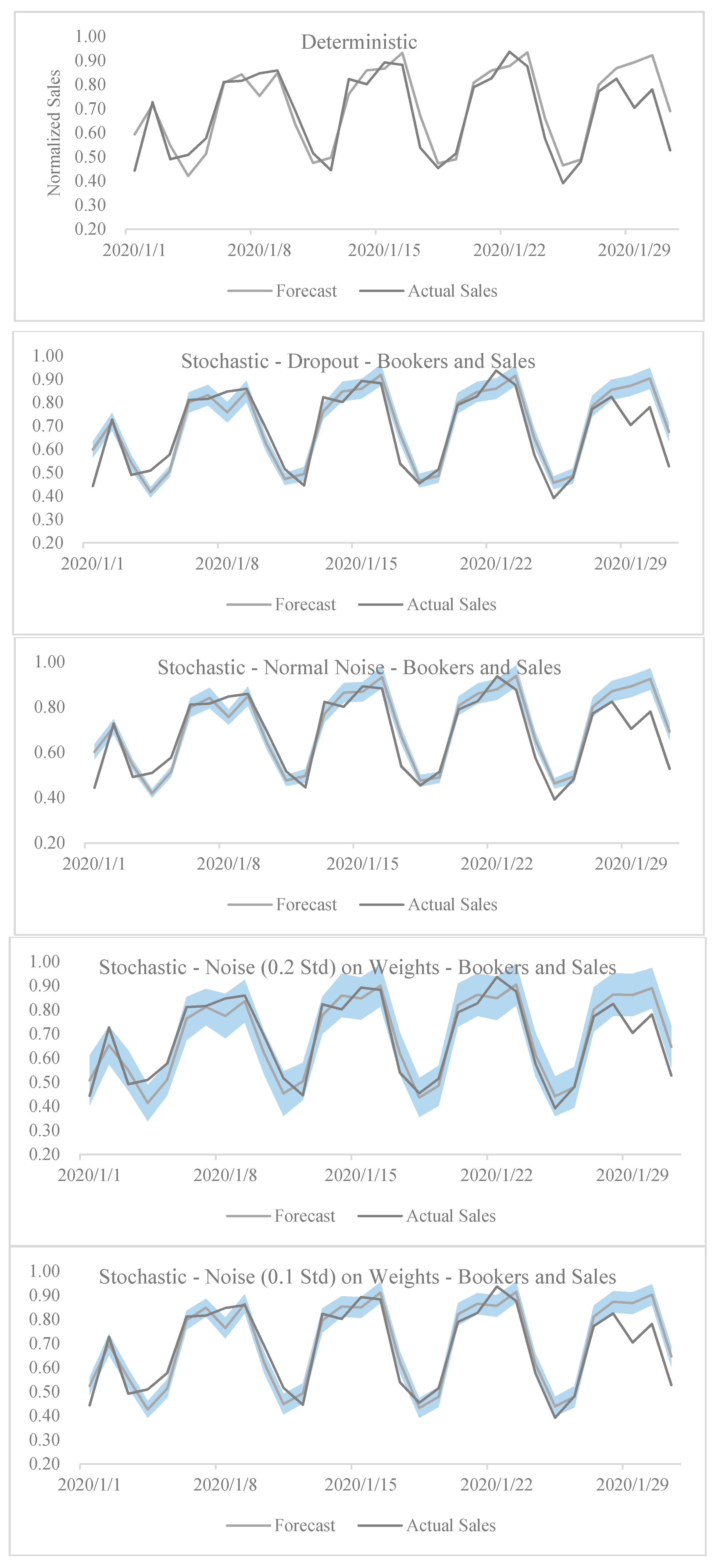
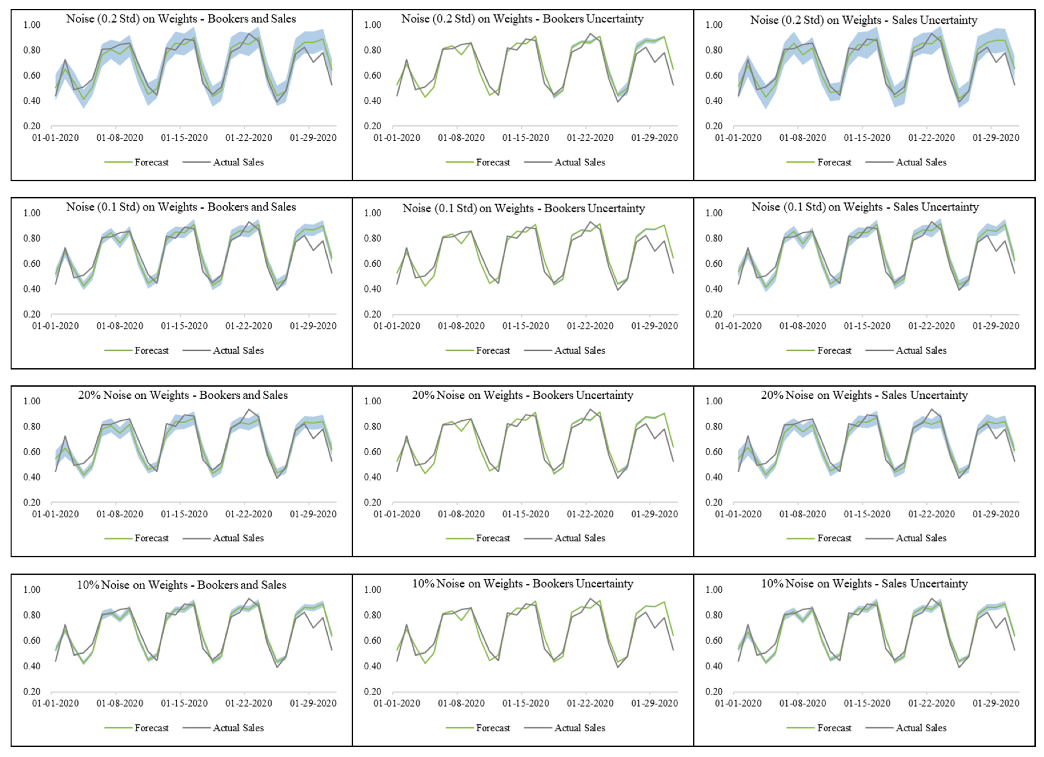
• 0 mean and fixed (0.1 and 0.2) standard deviation;
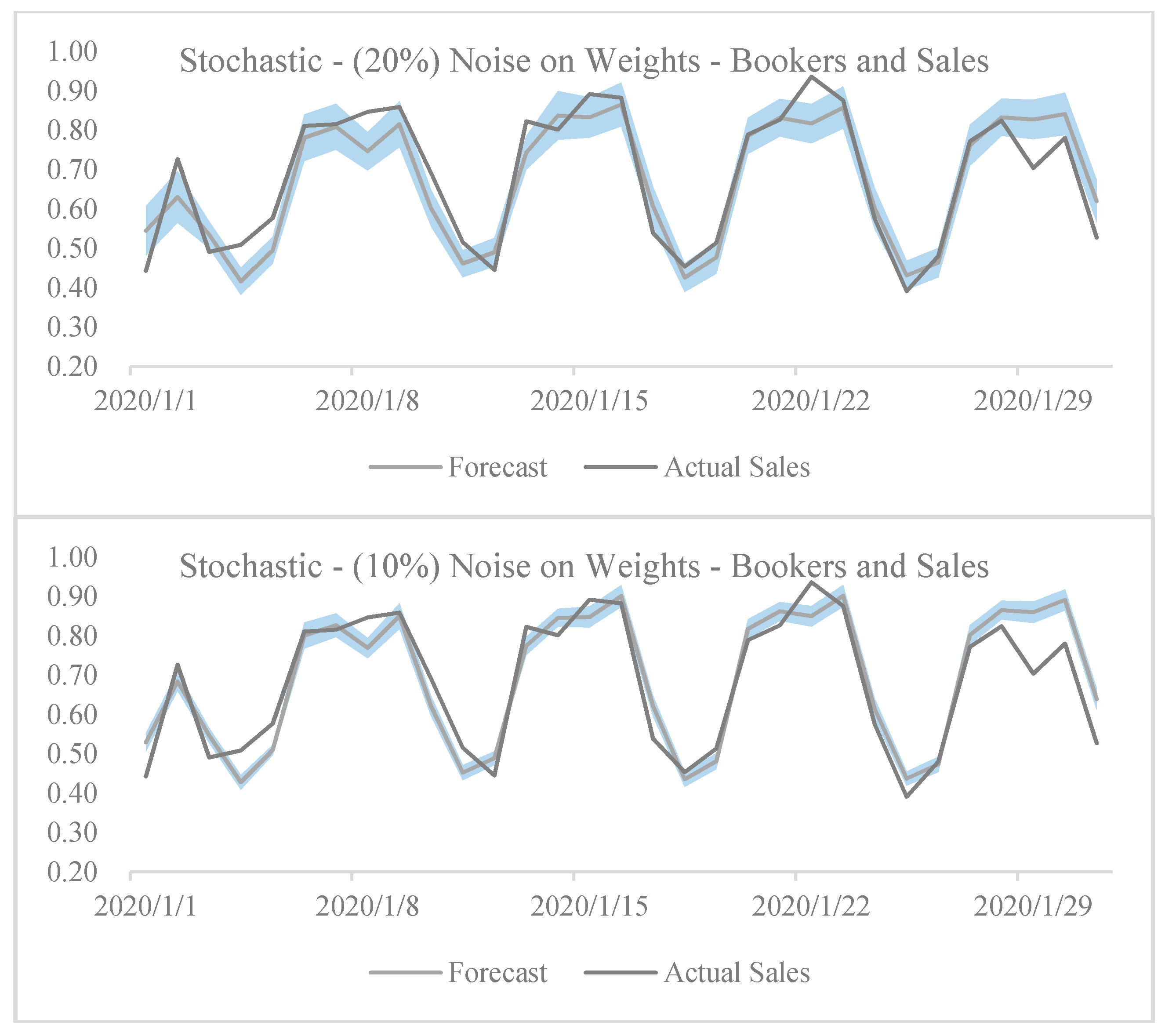
• 0 mean and fixed percentage (10% and 20%) of weight.

Then the three combination of models as described in the stochastic dropout approach (Case 2) were run for each of the two cases.

Historical, daily global hotels sales data from 1 January 2017 to 14 January 2020 were used for training the model. The forecasting models were trained on an 8-cpu Ubuntu Linux server with 32 gigabyte memory The percentage error between predicted sales vs. actual sales for the month of January 2020 was used as the error metric for the comparison of the performance of various models. This is referred to as observed error in

Table 1. Summary of sales forecast predictions for various approaches. * represents cases where the predictions are statistically significantly different from those of the deterministic model.

Model Description			Observed Error	p-Value of t-Test vs. Deterministic Model
Deterministic			4.02%	-
Stochastic—Dropout	Active Booker Count and Sales Uncertainty		2.81%	<0.001 *
	Active Booker Count Only Uncertainty		3.88%	<0.001 *
	Sales Only Uncertainty		3.10%	<0.001 *
Stochastic—Noise on Bookers and Sales	Active Booker Count Uncertainty	Normal Noise	4.17%	0.008 *
		Uniform Noise	4.50%	0.001 *
		Triangular Noise	4.16%	0.032 *
		Logistic Noise	4.13%	0.239
		Gumbel Noise	5.09%	<0.001 *
	Sales Uncertainty	Normal Noise	3.92%	0.240
		Uniform Noise	4.00%	0.877
		Triangular Noise	4.18%	0.558
		Logistic Noise	3.33%	0.043 *
		Gumbel Noise	8.00%	<0.001 *
	Active Booker Count and Sales Uncertainty	Normal Noise	4.12%	0.422
		Uniform Noise	4.47%	0.016 *
		Triangular Noise	4.02%	0.960
		Logistic Noise	4.68%	0.007 *
		Gumbel Noise	9.42%	<0.001 *
Stochastic—Noise on Weights	Active Booker Count and Sales Uncertainty	Noise STD: 0.1	2.13%	0.010 *
		Noise STD: 0.2	1.06%	<0.001 *
		Noise STD: 10%	1.48%	<0.001 *
		Noise STD: 20%	−1.58%	<0.001 *
	Active Booker Count Uncertainty	Noise STD: 0.1	2.45%	0.024 *
		Noise STD: 0.2	2.70%	0.067
		Noise STD: 10%	2.27%	0.014 *
		Noise STD: 20%	2.07%	0.008*
	Sales Uncertainty	Noise STD: 0.1	2.00%	0.002 *
		Noise STD: 0.2	1.40%	<0.001 *
		Noise STD: 10%	1.50%	<0.001 *
		Noise STD: 20%	−1.33%	<0.001*

4. Tests and Results

The models were evaluated on the total sales predicted for the month of January 2020 with the starting prediction date of 15 January 2020. Results of various model runs for conditions explained in the previous section are summarized in Table 1.

A quick look at the data shows that the best predictions are for the stochastic model with noise in weights (model constants) and worst for the case where noise is embedded in the input dataset. Within the latter case, worst predictions were observed for Gumbel noise distribution that modeled Generalized Extreme Value distribution. The predictions suggest that noise in the input dataset is not related to extremes and that no extreme (extraordinarily high or low) sale will happen. The sales predictions for models with noise in input variables (with the exception of Gumbel distribution) are very similar to the sales predictions of the deterministic model. This can be confirmed by analyzing the p-value of the two tailed t-test [36]. These results suggest that the current dataset does not have too much variation in input values and that active booker count and sales are close to being deterministic. In other words, there is very little uncertainty in the input dataset, and perturbation in the values does not alter the results (output sales forecast) significantly. Another possibility could be that noise in the input dataset does not follow any of the mathematical distributions used.

While the noise in input variables does not yield better predictions when compared to the deterministic model, randomly dropping the hidden units (neurons or cells) at each update during training using the dropout functionality of the LSTM model seems to improve predictions. The best predictions were observed when dropouts were applied to simulate uncertainty in both the active booker count and sales. This suggests that variability in the actual dataset is reduced by filtering out extreme values leading to better predictions. This contrasts with the case where every data point (and neuron) is included in training the LSTM models but with implicit uncertainty as demonstrated above.

The next step is to analyze the uncertainty in the model weights (model constants) coupled with dropouts in neural network layers, and its impact on sales predictions. The results summarized in Table 1 show that when noise was added to the model weights either as absolute value at 0.1 and 0.2 or as 10% and 20% deviation from the mean, the predictions were closest to the actual sales. The best observations were made for the case when noise with a standard deviation of 0.2 was added to the weights of both the active booker count and sales LSTM models. The p-values also indicate that predictions were significantly different from those of the deterministic model. Uncertainty in model weights seems to suggest that model convergence during training has more room to be worked on, or that the number of neurons and LSTM layers was not adequate. It is also possible that shallowness of the LSTM model in terms of fewer neurons and LSTM layers made model weights less deterministic.

For confidentiality reasons, sales numbers in this paper were scaled between 0 and 1; however, the variations in the actual and predicted sales numbers were preserved. The charts in Figure 5 show a comparison of predicted vs. actual sales on a daily level for the month of January 2020 for various versions of deterministic and stochastic models. Charts in Appendix A and Appendix B show the results of all the remaining possible combinations (active booker count only, sale only, and active booker count and sales) for the four cases given above.

Towards the end of the month (25 January onwards), we observed a deviation between predicted vs. actual sales. This happened because of the outbreak of corona virus. This had an impact on sales. The model overpredicted the sales because of the long-term memory, and it needed more data to build short term memory to realize the drastic impact of the virus on sales.

While it is worthwhile to understand the impact of uncertainty and noise in data on predictions, it would be interesting to extend the study to analyze the impact of corona virus spread on sales. One can determine the loss in sales by letting the model predict sales in the corona-free environment and then compare it to actual sales. Several such “what-if” simulations can be conducted using the models developed.

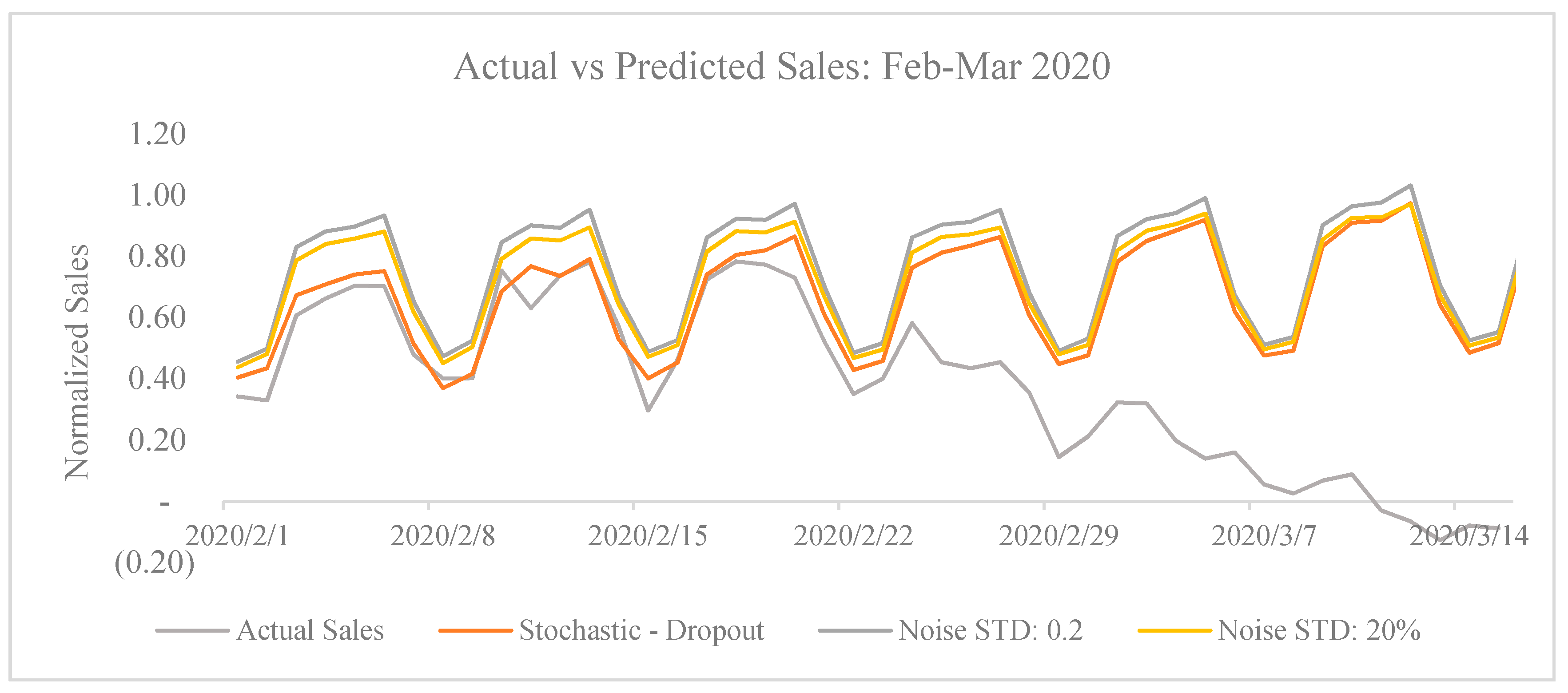
Impact of Corona Virus Outbreak on February 2020 and March 2020 Sales

Models with the best predictions, as determined in the previous section, were used to predict the sales for the months of February and March 2020. In other words, the following models were used:

• Stochastic dropout model with both active booker count and sales uncertainty;
• Noise in weights with 0.2 standard deviation in active booker count and sales models;
• Noise in weights with 20% standard deviation in active booker count and sales models.

For this study, a time-period that severely impacted the global sales due to corona virus outbreak, was chosen. The predictions were made on 15 February 2020, and then, the forecasts were compared with the actual sales to assess the impact of the corona virus outbreak.

Figure 6 shows that the impact of corona outbreak on sales was mild at the beginning of February, the impact became severe only in the last week of February.

Table 2. Impact of corona virus on sales.

Stochastic Dropout—Active Booker Count and Sales Uncertainty
Duration	Actual Sales	Predicted Sales	Business Impact
15 February to 29 February	7.46	9.90	−24.7%
1 March to 15 March	1.19	10.77	−89.0%
Total (15 February to 15 March)	8.65	20.68	−58.2%
Noise STD: 0.2 Active Booker Count and Sales Uncertainty
Duration	Actual Sales	Predicted Sales	Business Impact
15 February to 29 February	7.46	11.19	−33.3%
1 March to 15 March	1.19	11.62	−89.8%
Total (15 February to 15 March)	8.65	22.81	−62.1%
Noise STD: 20% Active Booker Count and Sales Uncertainty
Duration	Actual Sales	Predicted Sales	Business Impact
15 February to 29 February	7.46	10.66	−30.0%
1-March to 15-March	1.19	11.12	−89.3%
Total (15 February to 15 March)	8.65	21.78	−60.3%

summarizes the predictions for the loss in sales made by the three models discussed above.

The impact of the corona virus outbreak was extremely severe in March with a drop of 89.0% to 89.8% in sales till 15 March. The drop in sales in the second half of February was in the range of 24.7% to 33.3%. The loss for a one month period of 15 February to 15 March was around 58% to 62%.

Figure 7 shows that the LSTM model can predict the impact of corona virus on sales by adding a new binary input variable called the corona virus impact variable. The variable determines whether the sales are impacted by the virus spread or not. The model was quite accurately able to predict sales when the new variable was added. Sales were predicted to be substantially higher if the variable was not included in the model.

This study shows the power of LSTM based models to conduct “what-if” studies that otherwise would have been impossible to study in a real and practical environment. The same model can be used to understand how the sales would come back to normal levels once the menace of the virus has been conquered. The LSTM model can be integrated with models predicting when the impact of corona virus would end. Furthermore, the LSTM model can be used to perform sensitivity analysis to fathom differential change in sales with respect to differential change in the number of key account managers. This would allow the judicious hiring of key account managers. Similarly, we can study how much the increase in sales would be for every percentage increase in number of agencies (clients). Adding new variables to the model allows for the simulation of more scenarios. The possibilities are endless, and the use of complex and accurate machine learning techniques lend more credibility to the analyses.

5. Conclusions and Future Work

LSTM modeling is an effective technique that can be used in the travel industry as it is able to successfully model the nonlinear trends and variations in sales over time. Multiple ways of modeling uncertainties in an LSTM model are presented. Uncertainties can be modeled using dropouts as noise added to input variables and as gaussian noise added to the model weights. We observed that the prediction accuracy of an LSTM model can be improved by using dropouts, and even more effectively, by adding noise to the constants of the model. Uncertainty in the model weights has the biggest impact on the model predictions suggesting that reduced depth (number of layers) of the LSTM model can be compensated by adding noise to model parameters. Perhaps, a model with more neurons and LSTM layers would lead to more accurate deterministic predictions that would, however, require more data. The impact of corona virus on hotel business could be quantified, as the models have the flexibility to include or drop input variables, making LSTMs all the more desirable. While the sales forecasts were made at a global level, the same can be performed at the source market (country) level. Uncertainty in country-specific models can be researched, and a study can be conducted to see how these uncertainties correlate with the uncertainty at a global level. Models can be developed for other lines of business such as airlines, car rental, and sightseeing to name a few. The nature of uncertainties can then be compared across product lines. Owing to their credibility in generating accurate predictions, LSTM models can be used to study various hypothetical scenarios, the results of which can be trusted for business expansion.

References

1. Jiang, C.; Jiang, M.; Xu, Q.; Huang, X. Expectile regression neural network model with applications. Neurocomputing 2017, 247, 73–86. [Google Scholar] [CrossRef]
2. Castañeda-Miranda, A.; Castaño, V.M. Smart frost control in greenhouses by neural networks models. Comput. Electron. Agric. 2017, 137, 102–114, ISSN 0168-1699. [Google Scholar] [CrossRef]
3. Arora, S.; Taylor, J.W. Rule-based autoregressive moving average models for forecasting load on special days: A case study for France. Eur. J. Oper. Res. 2018, 266, 259–268. [Google Scholar] [CrossRef] [Green Version]
4. Hassan, M.M.; Huda, S.; Yearwood, J.; Jelinek, H.F.; Almogren, A. Multistage fusion approaches based on a generative model and multivariate exponentially weighted moving average for diagnosis of cardiovascular autonomic nerve dysfunction. Inf. Fusion 2018, 41, 105–118. [Google Scholar] [CrossRef]
5. Barrow, D.K.; Kourentzes, N.; Sandberg, R.; Niklewski, J. Automatic robust estimation for exponential smoothing: Perspectives from statistics and machine learning. Expert Syst. Appl. 2020, 160, 113637. [Google Scholar] [CrossRef]
6. Bafffour, A.A.; Feng, J.; Taylor, E.K.; Jingchun, F. A hybrid artificial neural network-GJR modeling approach to forecasting currency exchange rate volatility. Neurocomputing 2019, 365, 285–301. [Google Scholar] [CrossRef]
7. Castañeda-Miranda, A.; Castaño, V.M. Smart frost measurement for anti-disaster intelligent control in greenhouses via embedding IoT and hybrid AI methods. Measurement 2020, 164, 108043. [Google Scholar] [CrossRef]
8. Pradeepkumar, D.; Ravi, V. Soft computing hybrids for FOREX rate prediction: A comprehensive review. Comput. Oper. Res. 2018, 99, 262–284. [Google Scholar] [CrossRef]
9. Panigrahi, S.; Behera, H. A hybrid ETS–ANN model for time series forecasting. Eng. Appl. Artif. Intell. 2017, 66, 49–59. [Google Scholar] [CrossRef]
10. Buyuksahin, U.C.; Ertekin, Ş. Improving forecasting accuracy of time series data using a new ARIMA-ANN hybrid method and empirical mode decomposition. Neurocomputing 2019, 361, 151–163. [Google Scholar] [CrossRef] [Green Version]
11. Siami, N.S.; Tavakoli, N.; Siami, N.A. A Comparison of ARIMA and LSTM in Forecasting Time Series. In Proceedings of the 2018 17th IEEE International Conference on Machine Learning and Applications (ICMLA), Orlando, FL, USA, 17–20 December 2018; pp. 1394–1401. [Google Scholar] [CrossRef]
12. Helmini, S.; Jihan, N.; Jayasinghe, M.; Perera, S. Sales forecasting using multivariate long shortterm memory network models. PeerJ PrePrints 2019, 7, e27712v1. [Google Scholar] [CrossRef]
13. Graves, A. Generating sequences with recurrent neural networks. arXiv 2013, arXiv:1308.0850. [Google Scholar]
14. Zhu, L.; Laptev, N. Deep and Confident Prediction for Time Series at Uber. In Proceedings of the 2017 IEEE International Conference on Data Mining Workshops (ICDMW); Institute of Electrical and Electronics Engineers (IEEE), New Orleans, LA, USA, 18–21 November 2017; pp. 103–110. [Google Scholar]
15. Alonso, A.M.; Nogales, F.J.; Ruiz, C. A Single Scalable LSTM Model for Short-Term Forecasting of Disaggregated Electricity Loads. arXiv 2019, arXiv:1910.06640.2019. [Google Scholar]
16. Gal, Y.; Ghahramani, Z. Dropout as a Bayesian Approximation: Representing Model Uncertainty in Deep Learning. arXiv 2015, arXiv:1506.02142. [Google Scholar]
17. De Franco, C.; Nicolle, J.; Pham, H. Dealing with Drift Uncertainty: A Bayesian Learning Approach. Risks 2019, 7, 5. [Google Scholar] [CrossRef] [Green Version]
18. Kabir, H.D.; Khosravi, A.; Hosen, M.A.; Nahavandi, S. Neural Network-Based Uncertainty Quantification: A Survey of Methodologies and Applications. IEEE Access 2018, 6, 36218–36234. [Google Scholar] [CrossRef]
19. Akusok, A.; Miche, Y.; Björk, K.-M.; Lendasse, A. Per-sample prediction intervals for extreme learning machines. Int. J. Mach. Learn. Cybern. 2018, 10, 991–1001. [Google Scholar]
20. Ghahramani, Z. Probabilistic machine learning and artificial intelligence. Nature 2015, 521, 452–459. [Google Scholar] [CrossRef]
21. Krzywinski, M.; Altman, N. Points of significance: Importance of being uncertain. Nat. Methods 2013, 10, 809–810. [Google Scholar] [CrossRef]
22. Longford, N.T. Estimation under model uncertainty. Stat. Sin. 2017, 27, 859–877. [Google Scholar] [CrossRef] [Green Version]
23. Chen, G. A Gentle Tutorial of Recurrent Neural Network with Error Backpropagation. arXiv 2016, arXiv:1610.02583. [Google Scholar]
24. Ben Taieb, S.; Bontempi, G.; Atiya, A.F.; Sorjamaa, A. A review and comparison of strategies for multi-step ahead time series forecasting based on the NN5 forecasting competition. arXiv 2011, arXiv:1108.3259. [Google Scholar] [CrossRef] [Green Version]
25. Davies, R.; Coole, T.; Osipyw, D. The Application of Time Series Modelling and Monte Carlo Simulation: Forecasting Volatile Inventory Requirements. Appl. Math. 2014, 5, 1152–1168. [Google Scholar] [CrossRef] [Green Version]
26. Wright, W. Bayesian approach to neural-network modeling with input uncertainty. IEEE Trans. Neural Netw. 1999, 10, 1261–1270. [Google Scholar] [CrossRef] [PubMed]
27. Labach, A.; Salehinejad, H.; Valaee, S. Survey of Dropout Methods for Deep Neural Networks. arXiv 2019, arXiv:1904.13310. [Google Scholar]
28. Samuel, P.; Thomas, P.Y. Estimation of the Parameters of Triangular Distribution by Order Statistics. Calcutta Stat. Assoc. Bull. 2003, 54, 45–56. [Google Scholar] [CrossRef]
29. Gupta, R.P.; Jayakumar, K.; Mathew, T. On Logistic and Generalized Logistic Distributions. Calcutta Stat. Assoc. Bull. 2004, 55, 277–284. [Google Scholar] [CrossRef]
30. Qaffou, A.; Zoglat, A. Discriminating Between Normal and Gumbel Distributions. REVSTAT Stat. J. 2017, 15, 523–536. [Google Scholar]
31. Toulias, T.; Kitsos, C.P. On the Generalized Lognormal Distribution. J. Probab. Stat. 2013, 2013, 432642. [Google Scholar] [CrossRef] [Green Version]
32. Jiang, L.; Wong, A.C.M. Interval Estimations of the Two-Parameter Exponential Distribution. J. Probab. Stat. 2012, 2012, 734575. [Google Scholar] [CrossRef] [Green Version]
33. Ognawala, S.; Bayer, J. Regularizing recurrent networks—On injected noise and norm-based methods. arXiv 2014, arXiv:1410.5684. [Google Scholar]
34. Li, Y.; Liu, F. Whiteout: gaussian adaptive noise injection regularization in deep neural networks. arXiv 2018, arXiv:1612.01490. [Google Scholar]
35. Jim, K.-C.; Giles, C.; Horne, B. An analysis of noise in recurrent neural networks: Convergence and generalization. IEEE Trans. Neural Netw. 1996, 7, 1424–1438. [Google Scholar] [CrossRef] [PubMed] [Green Version]
36. Student. The Probable Error of a Mean. Biometrika 1908, 6, 1–25. [Google Scholar] [CrossRef]
Figure 1. High level pictorial representation of a Long Short Term Memory (LSTM) memory cell. where x t : Input vector at time t; a t : Input activation at time t as defined in Equation (1); i t : Input gate at time t as defined in Equation (2); f t : Forget gate at time t as defined in Equation (3); o t : Output gate at time t as defined in Equation (4); s t : Internal state at time t as defined in Equation (5); s t 1 : Internal state at time t − 1; o u t t : Model output at time t; o u t t 1 : Model output at time t − 1.
Make 02 00014 g001
Figure 2. Active Booker Count and Sales forecasting models and the relationship between the two.
Make 02 00014 g002
Figure 3. Sources and propagation of uncertainty in modeling techniques.
Make 02 00014 g003
Figure 4. LSTM Network with Dropout Cells.
Make 02 00014 g004
Figure 5. Actual vs. predicted January sales for various cases: deterministic model; stochastic—normal noise with active booker count and sales uncertainty; stochastic—dropout with active booker count and sales uncertainty; Stochastic—noise on weights—active booker count and sales. The details the of active booker count only stochastic models, and sales only stochastic models are shown in the Appendix A and Appendix B. The shaded area represents the range of stochastic variance (uncertainty) in the model predictions.
Make 02 00014 g005aMake 02 00014 g005b
Figure 6. Impact of corona virus outbreak on sales. Both the actual sales and model predicted sales in absence of corona virus are shown.
Make 02 00014 g006
Figure 7. Model predictions with and without the corona virus impact.
Make 02 00014 g007