Beyond Cross-Validation—Accuracy Estimation for Incremental and Active Learning Models


1
Research Institute for Cognition and Robotics, Bielefeld University, 33615 Bielefeld, Germany
2
HONDA Research Institute Europe GmbH, 63073 Offenbach, Germany
*
Author to whom correspondence should be addressed.
Mach. Learn. Knowl. Extr. 2020, 2(3), 327-346; https://0-doi-org.brum.beds.ac.uk/10.3390/make2030018
Submission received: 14 July 2020
/
Revised: 8 August 2020
/
Accepted: 24 August 2020
/
Published: 1 September 2020
Abstract
:For incremental machine-learning applications it is often important to robustly estimate the system accuracy during training, especially if humans perform the supervised teaching. Cross-validation and interleaved test/train error are here the standard supervised approaches. We propose a novel semi-supervised accuracy estimation approach that clearly outperforms these two methods. We introduce the Configram Estimation (CGEM) approach to predict the accuracy of any classifier that delivers confidences. By calculating classification confidences for unseen samples, it is possible to train an offline regression model, capable of predicting the classifier’s accuracy on novel data in a semi-supervised fashion. We evaluate our method with several diverse classifiers and on analytical and real-world benchmark data sets for both incremental and active learning. The results show that our novel method improves accuracy estimation over standard methods and requires less supervised training data after deployment of the model. We demonstrate the application of our approach to a challenging robot object recognition task, where the human teacher can use our method to judge sufficient training.
1. Motivation
Estimating the classification accuracy of a machine-learning model is particularly important in incremental and life-long learning tasks, where a continuous stream of new training data adapts the classifier state over time. We can imagine service robots that will adapt to their application environment by continued human teaching and error correction to improve their performance during operation. Current examples are vacuum or mowing robots that may already have some limited adaptivity to the spatial working area layout and configuration. It could be very helpful to allow a home user to incrementally teach those service robots how to deal with special obstacles or objects in the home environment. Consider for example an autonomous lawn mower with a camera for object recognition in the garden. The robot mows the lawn at regular intervals and concurrently stores views of objects which were encountered during operation. Occasionally the robot will ask the user to classify the objects and how to deal with them (e.g., “mow over leaves but avoid flowers”). This raises the question when the robot is good enough in object recognition to fulfill this task autonomously. To limit the teaching effort, it first makes sense to choose requested labeling examples according to standard active learning approaches. These methods select those training examples that offer the largest expected performance gain. Secondly, additional training data is only needed to be requested as long as the classifier accuracy is below a user-defined threshold. This requires a robust estimation of the current accuracy. Also, if the system accuracy does not improve with additional labeled data, the task cannot be carried out autonomously by the robot [1].
The research topics of incremental and life-long learning have gained more attention in recent years. Humans and animals are especially good in perceiving, integrating and transferring information from continuous data streams. In this article, we are interested in the special topic of accuracy estimation for an incrementally learning classifier. This is highly relevant information for initiating and managing the learning process.
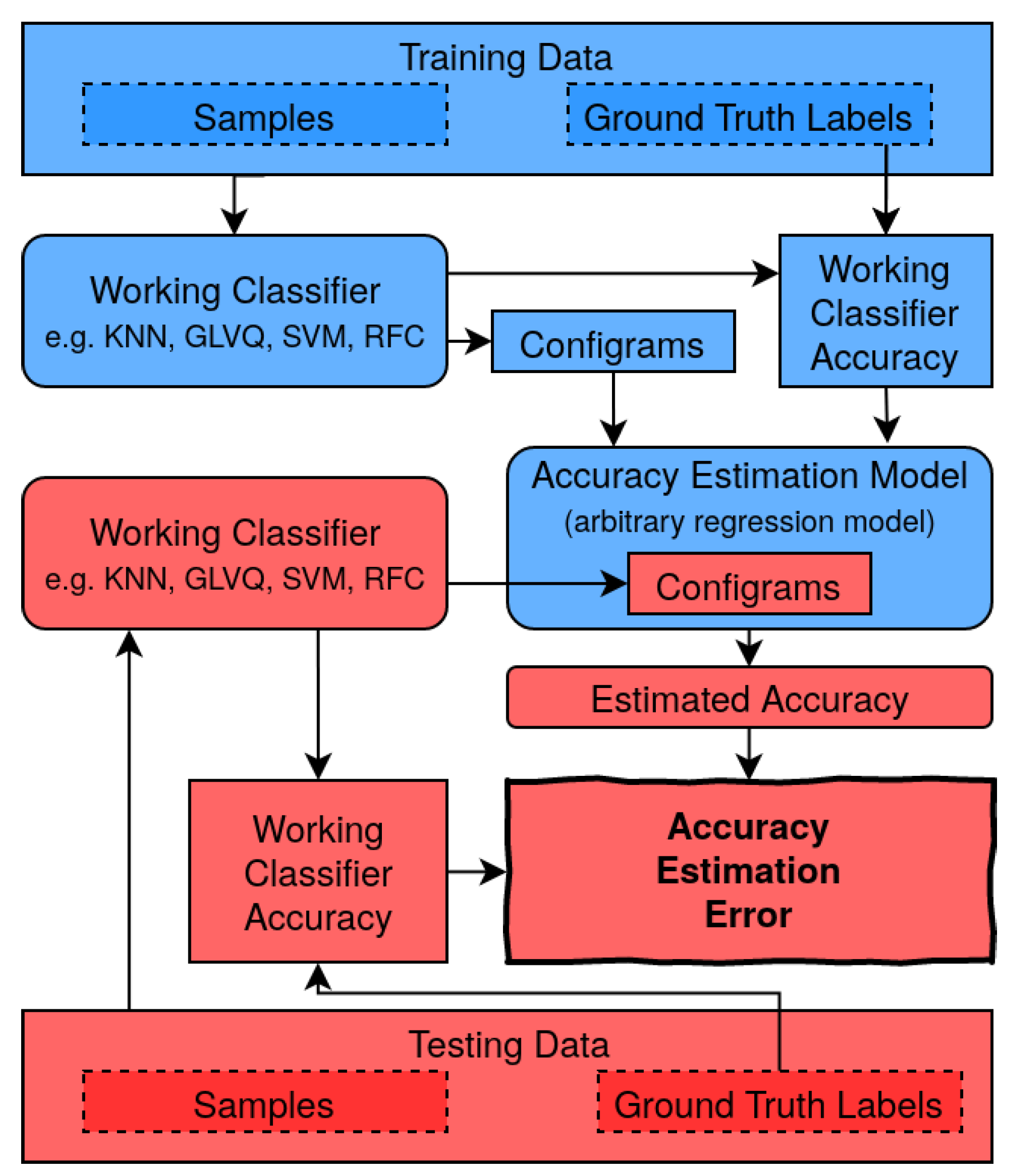
Our approach is to train a regression model using the confidence information of an arbitrary classification model to predict its accuracy on a test set with only a fraction of supervised labeled data. This semi-supervised technique allows us to predict the classifier’s accuracy while training (also illustrated in Figure 1). So, our goal is to determine it in each stage of training and not only to predict the final accuracy after training is completed like in most of the other related work. The selection of training data has a strong influence on the classifier accuracy gain, which is well-known from active learning research [2]. We investigate the relation of this effect towards the estimation of the incremental classifier performance. However, no new methods for active learning are proposed here, we rather analyze the problematic effect of active query strategies on using standard supervised accuracy estimation techniques.
We evaluate our method on several analytical and real-world data sets and within an object recognition task, both with random and active querying, where uncertainty sampling is used to select the most uncertain samples for training. Our algorithm clearly outperforms cross-validation (CV) and interleaved test/train error (ITT) in both cases but especially while querying actively. To further motivate our approach, an incremental life-long learning experiment is simulated, where new data is inserted while training and the accuracy estimation module is used to determine the time of retraining to achieve a minimum desired task accuracy.
2. Related Work
Accuracy estimation for classification algorithms can be considered to be a tool for judging the suitability of machine-learning methods for certain applications. Since this is a subdomain of the rising research field of explainable artificial intelligence (XAI), we first position our work in relation to this. We then discuss recent approaches for accuracy estimation in offline or batch learning and finally review methods applied for online or incremental learning.
In recent years, the research field of explainable artificial intelligence (XAI) has gained a lot of attention [3,4,5]. The key goals of XAI are to determine if or if not an AI system satisfies application-centered requirements [6] and to explain why it behaves as it does [4]. The latter question becomes more and more important today, since generic models like deep neural networks have become more and more complex. This complexity induces opaqueness about which feature leads to a decision [7] or what characteristics of a sample is responsible for a certain model output [8]. Our focus is an estimation of how well an AI system for classification will perform. Being able to answer this question is essential for human users to build trust in the reliability of the model [9,10,11].
The reliability of a classifier can be quantified by computing accuracy on a hold-out test set or by accumulating confidences from predicting single examples [12]. While probabilistic classifiers have an integrated confidence prediction, non-probabilistic models are using model-specific heuristics estimating confidences (see Section 4). There are also model-agnostic approaches for estimating confidences like Conformal Prediction [13]. Jiang et al. suggest comparing the output of any classifier with a high-density nearest neighbor model to get high quality confidence estimates [14].
Let us now review approaches for accuracy estimation in offline settings. Platanios et al. [15] estimated classifier accuracy by considering the agreement rate of multiple classifiers of different types trained with independent features, possibly underestimating performance gains using all features. Another recent approach by Donmez et al. [16] is also applicable with a single classifier but requires the label distribution for evaluating a maximum likelihood. This is applicable, e.g., for medical diagnosis or handwriting recognition, where the marginal frequency of each class is known. Aghazadeh and Carlsson [17] proposed a method to determine the quality of a train and test set by evaluating local and global moments for each class, like intra-class variation and connectivity. They evaluated this fully supervised approach via a leave one out cross-validation on Pascal VOC 2007 and could predict the final mean absolute error (MAE) of the held-out class with about 4–5% accuracy. Welinder et al. [12] showed that it is possible to estimate a binary classifiers precision and recall class-wise by fitting a mixture model per class in a histogram of confidences and sample those mixture models with various techniques. This comes closest to our problem setting but it is most likely only applicable on binary classification problems.
After discussing offline learning approaches let us now focus on incremental learning scenarios. Artificial models can be fragile if they cannot access the entire training data at once [18,19]. Catastrophic forgetting [20,21] describes the problem of new information suppressing information from earlier training. Especially if new classes occur during training this is a problem [22]. Another problem can be imbalance of data [23] that is quite natural for, e.g., a robot that acquires a high proportion of samples of one particularly “dominant” class and must be, therefore, very attentive for classes that it perceives rarely. Concept drift [24,25] describes the problem of sample distributions that change over time. This can be an abrupt event in the data stream, but it also can be a gradual, reoccurring or even virtual process [26]. Gomes et al. [27] mention other possible research directions within incremental learning like anomaly detection [28], ensemble learning, recurrent neural networks and reinforcement learning.
Active learning is an efficient technique for incrementally training a classifier. One variant is pool-based active learning, which is also evaluated later in this manuscript. By using a querying method for selecting useful unlabeled samples for training, it is possible to boost the training process. There are a variety of querying approaches for finding the best samples to be queried [2]. An often-used querying technique is uncertainty sampling [29] which requests the samples with the least certainty for labeling. Other strategies select samples based on the expected model output change [30], or they consider a committee of different classifiers [31] for choosing the samples to be queried. A current trend is to train data-driven approaches for querying [32,33].
Although these are the main research fields in incremental and active learning, comparably less research has been done related to accuracy estimation in incremental or active learning, which requires the accuracy estimation model to adapt to an evolving classifier. A common choice for estimating the accuracy in incremental learning is storing a fraction of the labeled training data and to perform a cross-validation [34]. Another common approach is called interleaved test/train error [19,35]. It requires a classification of each new sample before using it for training. The classifier’s accuracy is then estimated by averaging over a window of past classifications. However, both approaches solely estimate the accuracy based on labeled instances. In the following we investigate a novel semi-supervised approach that also takes confidences on unlabeled data into account.
3. Accuracy Estimation of Incrementally Trained Classifiers
In this contribution we want to answer the following question: “How can we best estimate the current accuracy of an incremental learning classifier, taking previous learning sessions into account?”
We wish to create an accuracy estimator for a classifier trained by incremental learning. In such a setting one frequently wishes to monitor the accuracy of the classifier as more and more training examples are added (e.g., in order to be able to stop learning when a requested accuracy threshold is surpassed). Ideally, changes in accuracy can be detected that may be caused by changes in the statistics of the data (e.g., when dynamically adding new or removing existing classes).
Although it is straightforward to detect such accuracy changes by permanently sampling many examples and querying their labels, this straightforward strategy may be too expensive for many applications. Therefore, we aim for an estimator that can predict the accuracy of the trained classifier on the basis of a sufficiently large sample of unlabeled examples (compare Figure 1). Such an estimator could then predict accuracy changes of a trained classifier under changes of the pool of unlabeled examples. For instance, changes in the relative frequencies of examples that are associated with particular classes, or addition of new examples which represent existing classes in modified ways. Obviously, such a flexible accuracy monitoring that is based only on unlabeled examples is of high value in many applications (one specific example is presented in Section 6).
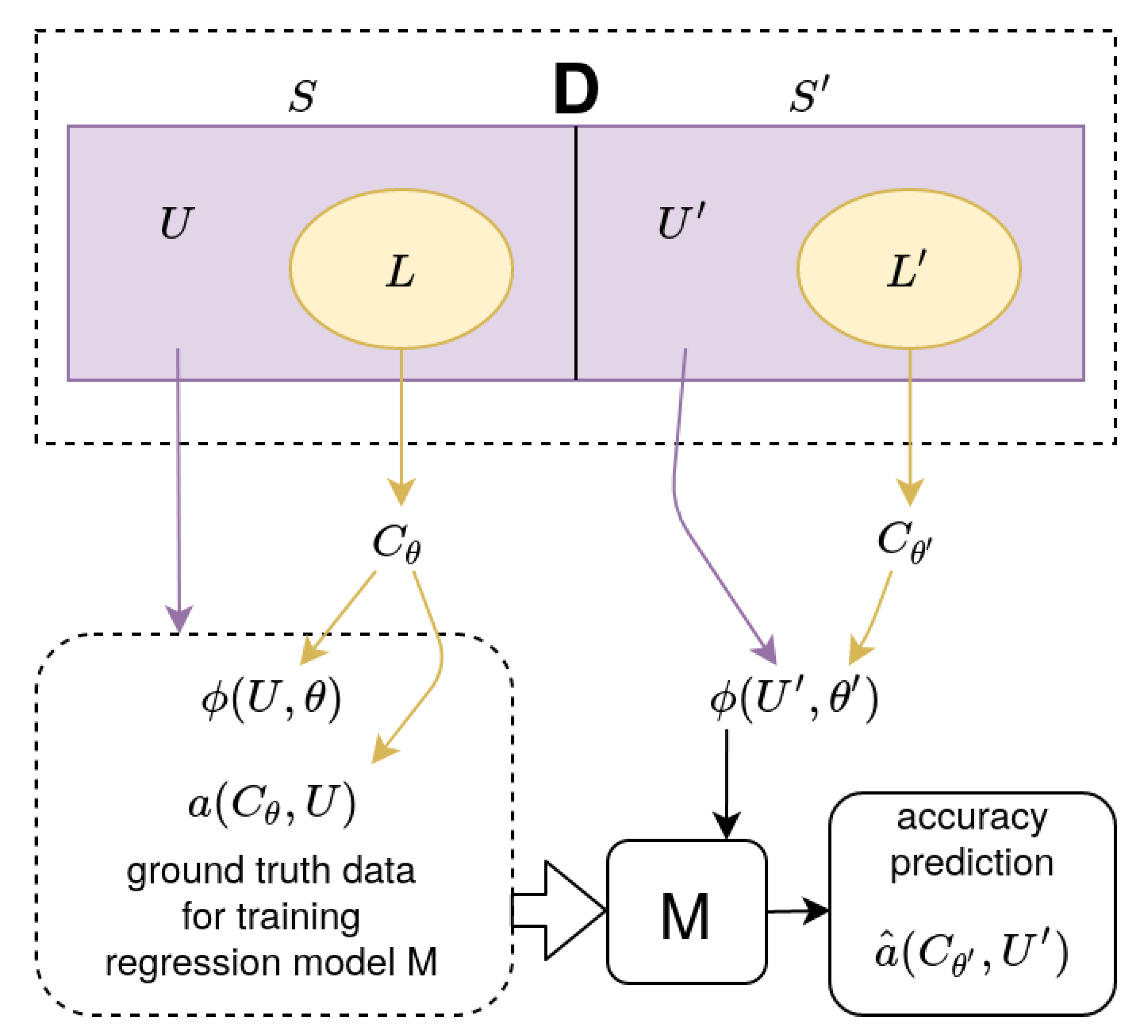
To fix our notation we denote by D the data set that characterizes our domain. Subsets S and denote possible training data pools within D (see Figure 2). Each subset consists of an unlabeled pool () and a labeled pool ().
We make use of a standard incremental learning paradigm [19] to train an incremental classifier either with random or active sampling.
The beginning of training starts with an empty L. A querying function selects samples, either randomly or uncertainty-based, from the unlabeled set U in mini-batches with size B. These batches are labeled by an oracle. This is in most cases a human annotator, whereas in our experiments ground-truth label data were used. As the training progresses, samples from the unlabeled pool U are labeled and moved into the labeled pool L. Simultaneously, the classifier C is trained online with the new labeled batch. The classifier is trained with N batches.
Formally, the classifier is given as a function that maps some unlabeled data item u into its class label y. In the following, it will be denoted as working classifier and denotes its adaptive parameters. Additionally, it is required that the working classifier comes with a confidence measure that reflects the reliability of its output on a given input item u when training led to parameters . Section 4 outlines some classifiers which were used in the evaluation together with their unique approaches for .
The construction of the accuracy estimator M for the chosen working classifier requires the one-off solution of an associated learning or regression task. After that the estimator becomes available for subsequent monitoring of incremental training of various instances of the chosen same working classifier. As will be seen shortly, this associated regression task will make use of some initial incremental training runs of several working classifier instances to generate the ground-truth data to compute the regression model that provides M.
Formally, the accuracy estimator M will have to map from a suitably chosen input feature vector . This input feature vector captures information about the accuracy of the working classifier with parameters when classifying samples from the pool U. The accuracy value is the desired output of the desired mapping (for M the explicit notation of its own adaptive parameters is omitted).
The input feature vector is obtained from confidence histograms (“configrams”) that are computed from the working classifier’s confidence measure as follows: J-dimensional confidence histograms over “confidence bins” of width in the confidence interval [0,1] are created, based on sampling a “representative” subset of our data pool. The histogram count of bin j, , is thus given as
with the bin membership indicator function
and U a suitably large subset of D. Each histogram will be a single input point for the regression model M. To determine this model, many such points are needed.
For the monitoring, the model must be appropriate for working classifiers in different incremental states. Therefore, configrams are created not for just a single, but instead for a sequence n = 1,2,…N of different such training states. This sequence is obtained in a similar fashion as in the later application: samples from the data pool are grouped into mini-batches which are counted by the index n. Each new mini-batch leads to an incremental update of the working classifier with changed adaptive parameters and corresponding histogram counts (that now depend on training state n together with bin number j). This generates a sequence of input feature vectors component-wise given as:
with the bin membership indicator function
Finally, each training state n and sample u requires checking of whether the prediction coincides with the true label or not:
The average
represents the ground-truth accuracy that belongs to histogram vector (note that this last step of ground-truth computation for the regression model requires the access of all labels in subset ). Finally, all and become concatenated into two vectors. To generate more of these configram-accuracy pairs, not only one classifier instance but a classifier ensemble with Q instances of the same classifier is trained with different initializations (random queries from ).
After training the ensemble of classifiers and collecting several configram sets, they are stacked to a feature vector . Analogously the ground-truth accuracies are stacked to a vector . The accuracy estimator M is an arbitrary regression model, trained with as features and target values.
Once the Configram Estimation Model (CGEM) M has been obtained, it can be applied to further incremental learning tasks. These are drawn from the domain D that may use pool whose statistics may differ from the “model-training” pool . The model will then extrapolate what is has learned from about the relationship between configrams and output accuracy of an incrementally trained working classifier instance. Therefore, it permits on very quick accuracy predictions without needing to query any labels in . This extrapolation assumes that the domain D is sufficiently homogeneous so that new pools drawn from D have a high likelihood to be sufficiently similar to the model-training pool S to admit the above accuracy extrapolation through the model M. The workflow of training and applying M is also visualized in Figure 3.
Also note that two different quality measures are discussed: the accuracy of , defined as Working Classifier Accuracy (WCA). And—as a more important quality measure for this contribution—the error estimated with M on test set and denoted Accuracy Estimation Error (AEE). It is defined as
For M common regression models [36] were tested, like a neural net (mlp), nearest neighbor regression (NNR), ridge regression (ridge), XGB regression (XGB), gaussian process regression (GPR) and support vector regression (SVR).
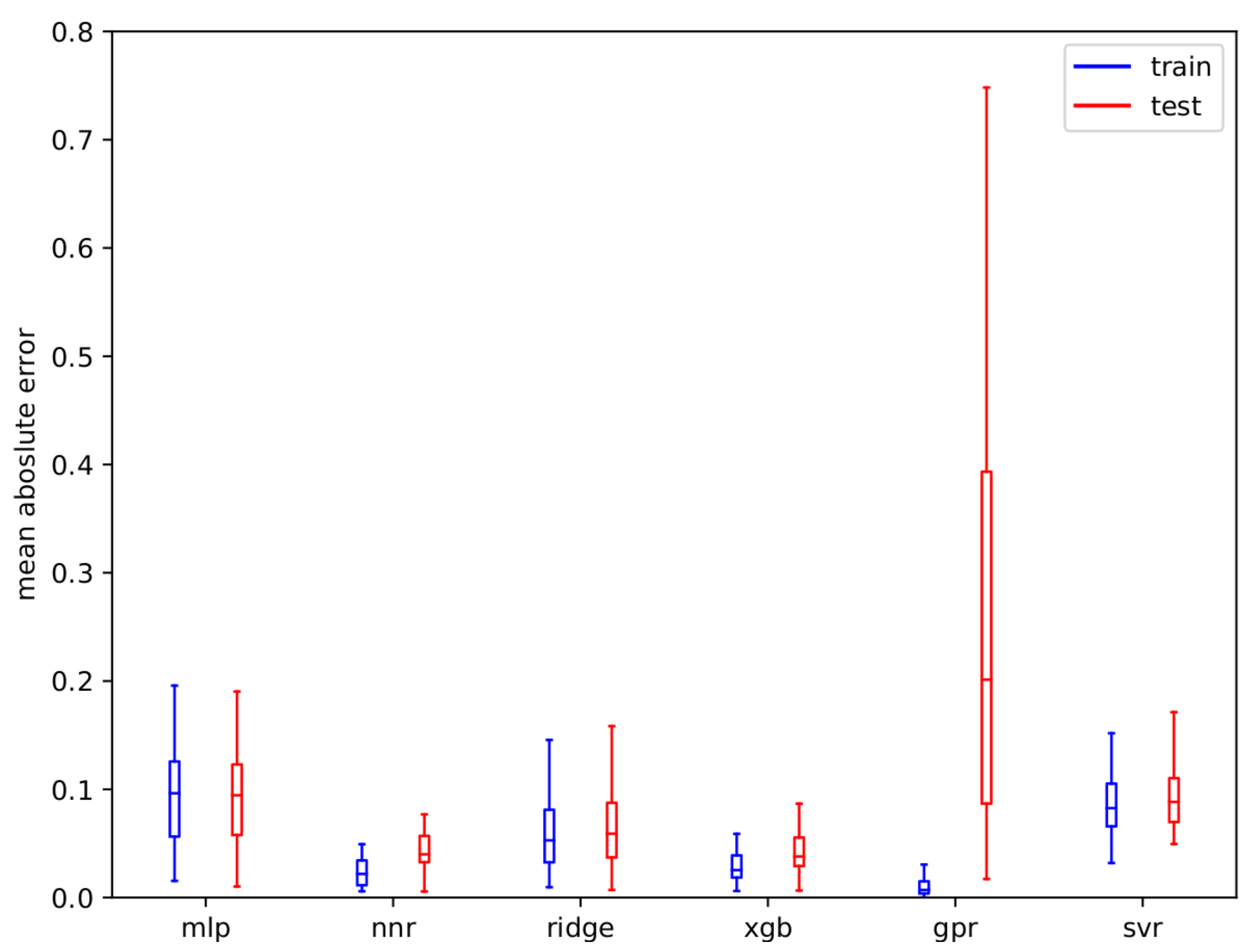
The different regression models were compared by evaluating them on collected configram-accuracy-pairs from trainings of all tested working classifiers on all data sets that are evaluated later in this article in Table 4. The averaged AEE of all models is displayed in Figure 4 where the performance of the models for both the training set with blue boxes (this is the training error for estimating the configrams used for training the model itself) and on the test set with red boxes is shown. Although GPR has the lowest AEE on , the model is highly overfitting and thus has by far the largest error on . We experienced that regression using the neural net (mlp) can deliver high performance for certain configrams, but is under-performing on others. Also, we experienced a high oscillation of accuracy in terms of the number of trained epochs. Nearest neighbor regression (nnr) is the most reliable approach on our data, so we select nnr to be used in our further evaluation as the overall best performing regression model.
4. Set of Classifiers and Their Confidence Estimation
We denote our target classifier as C and choose four different classifiers (KNN, GLVQ, SVM, RFC) for our evaluation. In our experiments KNN and GLVQ are trained in an online fashion. Especially GLVQ is explained here in depth because it is not so well known but past research has shown that it fits well in our incremental learning setting. SVM and RFC are retrained in an accumulated way after each trained batch on L. Each classifier has a unique way of estimating its confidence and this will reflect how the configrams will look like.
4.1. Support Vector Machine (SVM)
A Support Vector Machine (SVM) [37] is a maximum margin classifier, separating classes using a hyperplane defined by a linear combination of so-called support vectors. In our experiments a one-vs-all encoding is used, where one SVM is trained for each class as positive and all other classes as negative, for supporting multi-class classification. A popular way for estimating classifier confidences is the Platt Scaling [38], that fits a sigmoid function mapping the SVM’s outputs to probabilities.
4.2. Random Forest Classifier (RFC)
A Random Forest Classifier (RFC) [39] is an Ensemble of Decision Tree Classifiers (DTC). A DTC is trained by determining the most important features and placing them in a tree-wise structure. The classification-labels are in the leaf notes. As the splitting measure for finding the most important features the Gini Index is chosen. The confidences are estimated by determining for each leaf node the fraction of training samples of the same class.
4.3. k-Nearest Neighbors (KNN)
kNN is an instance-based classifier which simply memorizes samples . The classification of an unlabeled sample is done by determining its k-nearest samples within together with their given labels and distances to u: . Normalized weights are determined for n by: . The winning class p is estimated by denoting all unique labels as z. The confidence estimates is calculated with .
4.4. Generalized Learning Vector Quantization (GLVQ)
GLVQ [40] is using so-called prototypes to represent data. They are interpretative, the number of classes does not have to be known beforehand, no complete retraining is necessary and efficient techniques for querying new samples in active learning were studied before [41].
GLVQ is derived from LVQ, which is also instance-based but more memory efficient compared to kNN, because several samples are represented by a single prototype. In LVQ, as originally proposed by Kohonen et al. [42], data set D is modeled through p prototypes and their assigned labels for k classes. Notice that p and k can be varying during training. An input sample is classified by choosing the label of the nearest prototype, where the Euclidean distance is used. During supervised training, the algorithm adjusts the position of the prototypes so they model the training set optimally. An efficient variant is generalized LVQ. The prototype positions are updated via the rules and where is the prototype of the true class and is the nearest prototype of another class, and are their corresponding distances to x. Sato et al. [40] suggest to set and to use a relative distance for :
Performing a prototype position update as above is equivalent to a stochastic gradient descent. We reformulate to an unsupervised measure
where is the distance to the nearest prototype and is the distance to the next nearest prototype of another class. With this we calculate confidence estimates:
5. Evaluation
We evaluate the CGEM approach on static analytical data sets and show properties on drifting analytical data. We further evaluate a variety of real-world data sets and we finally test CGEM in a simulated human–robot interaction experiment.
For evaluating the regression model M, the data set D is split into an equal sized train set S and a test set S’ randomly. For training M, the classifier ensemble is trained on S with mini-batches for the analytical experiments and with mini-batches for the real-world experiments. Each batch has the size samples. The regression model M is trained as described earlier. To test M, a second classifier ensemble is trained on S’, analogously to the training of C before. After each trained batch of , the configrams were extracted for evaluating M. Also, two baseline methods are evaluated for comparison: interleaved test/train error (ITT) and stratified 5-fold cross-validation (CV) where the implementation of the sklearn python package is used. For the window size parameter of ITT, we found out that 30 is a good value. If too few samples are in the labeled pool in the early stage of training, both the number of folds for CV and the window size for ITT are adjusted to a lower number.
As mentioned earlier we deal with two different quality measures. On the one hand we evaluate the Working Classifier Accuracy (WCA) of after training for N batches. More important for us in this contribution is the Accuracy Estimation Error (AEE) which we define as the mean absolute error (MAE) of the respective accuracy estimation approach compared to the ground-truth accuracy, both computed on . This is evaluated after each trained batch and averaged over all N batches for defining a mean accuracy over the entire training of .
For our analytical experiments a classifier ensemble with instances of the same classifier is used and each experiment is repeated times with a shuffled train test split (only for static data) to average our results. For the real-world experiments instances of the same classifier are trained, and each experiment is repeated times since these experiments were significantly more resource-intensive.
5.1. Analytical Static Data Sets
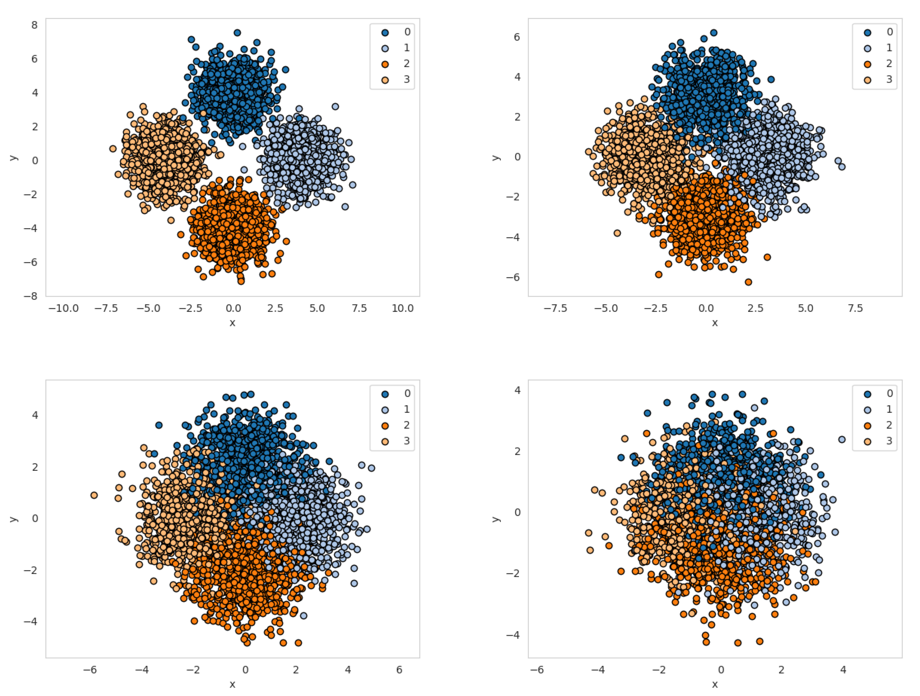
In our first evaluation step we choose to classify samples drawn from four Gaussian distributions (“Four Gaussian data set”). All Gaussian distributions have a standard deviation and are located on a circle with various radii (see Figure 5).
The final Working Classifier Accuracy (WCA) after training the classifiers is listed in Table 1. Also, an Optimal Bayes Classifier (OBC) is evaluated to provide the best possible WCA on the respective data set.
The classifiers’ performance is mostly comparable on all data sets. On r1, the data set with the largest overlap, KNN and RFC performed worse.
The mean Accuracy Estimation Error (AEE) can be seen in Table 2. CGEM is outperforming cross-validation (CV) and interleaved test/train error (ITT) by a significant margin. As expected, with a smaller r (i.e., a harder classification problem), AEE is getting higher for all tested approaches, this is similar for CV and ITT.
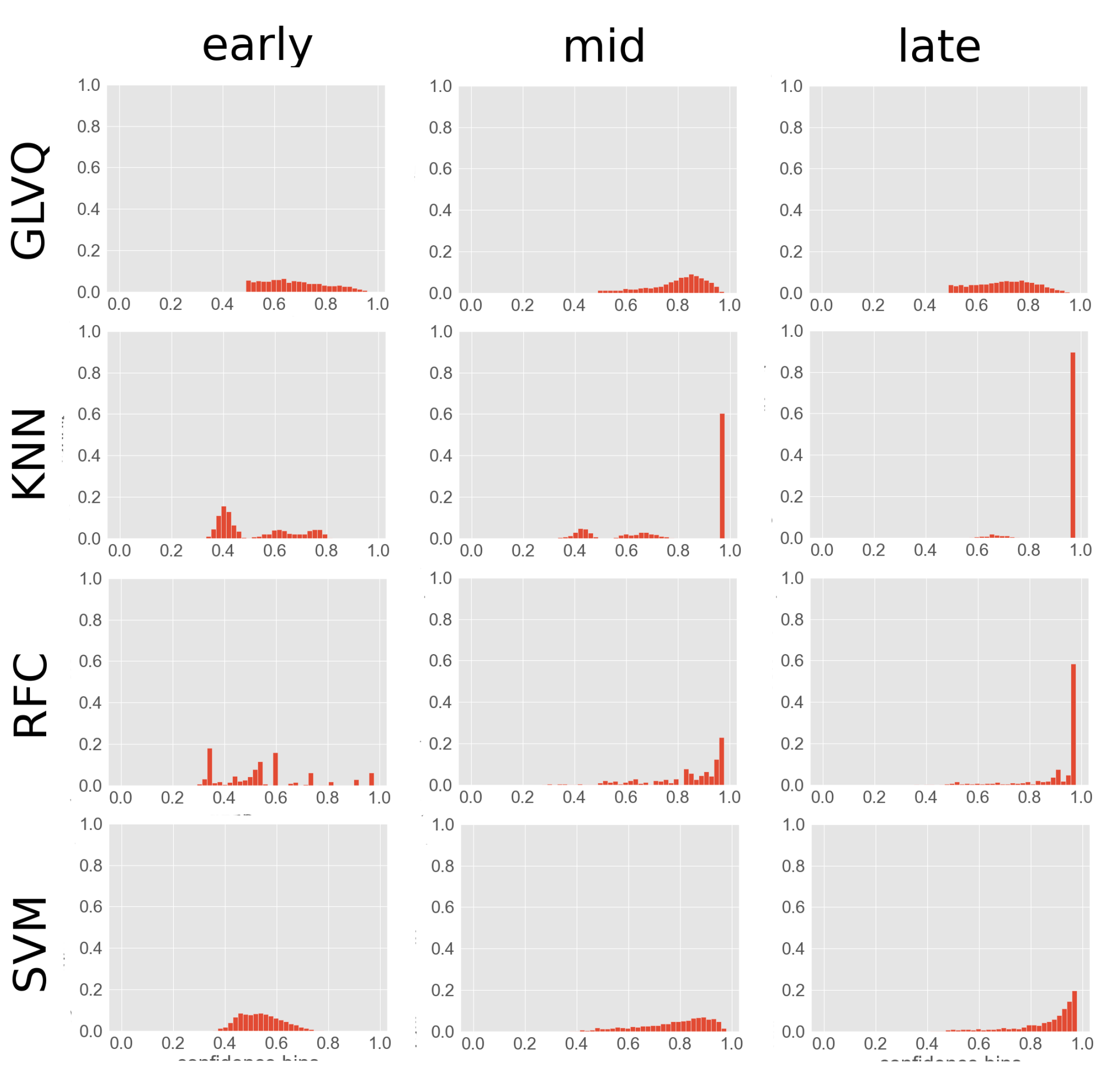
To better understand CGEM, several configrams from the Four Gaussians r3 data set were visualized in Figure A1. It is visible that during training the confidences are shifting nearer to 1. An exception is the GLVQ classifier, which is in our case first placing prototypes for representing classes (mid plot) and then moving those prototypes (late plot). M needs to adapt to this. GLVQ also has the flattest configrams, which may also explain the poorer performance compared to the other classifiers.
5.2. Analytical Drifting Data Sets
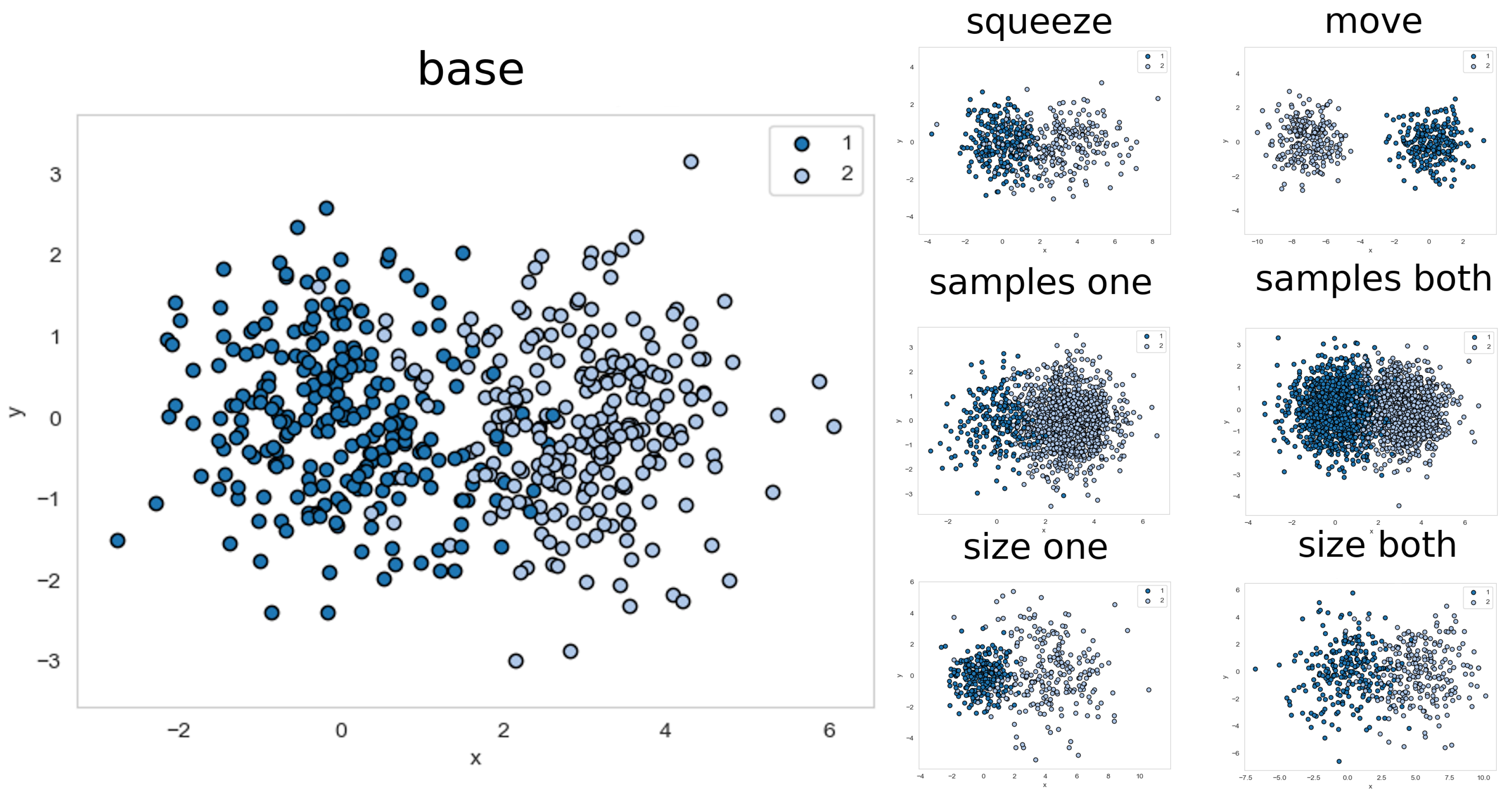
We also want to show properties of CGEM with drifting data, where it is assumed that S’ is drawn from a different distribution that ’drifted away’ from S. This evaluation sections uses a different setting as described earlier. Here, a base data set is used consisting of two classes and , which were sampled from Gaussian distributions as pool S with 500 samples per class (see Figure 6 top). Both distributions are isotropic with standard deviation of , and the means and . The base data set is then modified in 6 different ways and with 6 different intensities each (see Figure 6) for use as S’. The maximum intensity is denoted as , where all other intensities are sampled uniformly from the respective parameter of the base data set to (which is described in the following list).
- one size: is multiplied by 2. Translating by ensures that both classes have the same margin.
- both size: and are multiplied by 2. To ensure that both classes have the same margin is translated by .
- one samples: number of samples drawn from are multiplied by 5.
- both samples: number of samples drawn from and are both multiplied by 5.
- move: is translated by .
- squeeze: is multiplied by 3
The AEE is mostly affected by moving one class (see Table 3). By moving one class over the other the quality decreases until both classes are in the same spatial relation as in the base set, leading us to the assumption that it is only important to have roughly the same relations between classes. Squeezing one class is also affecting AEE negatively because the amount of overlap changes.
5.3. Real-World Data
5.3.1. Data Sets
We used five real-world data sets in this part of the evaluation. For WDBC [43] no preprocessing was done at all. For CALTECH101 [44], PASCALVOC2012 [45] and OUTDOOR [35] the VGG19 deep convolutional neural net [46] was used without the last SoftMax layer and with the weights from the image net competition as a feature representation. For extracting facial features for CELEBA [47] dlib (http://dlib.net/) was used. The target at CELEBA was to differentiate between males and females.
5.3.2. Incremental Learning
The accuracy estimation error (AEE) from incremental learning with random querying can be seen in Table 4. CGEM is outperforming the baseline methods in nearly all cases with an AEE of 2.3% to 4.0%. The final working classifier accuracy (WCA) is shown in Table 5.
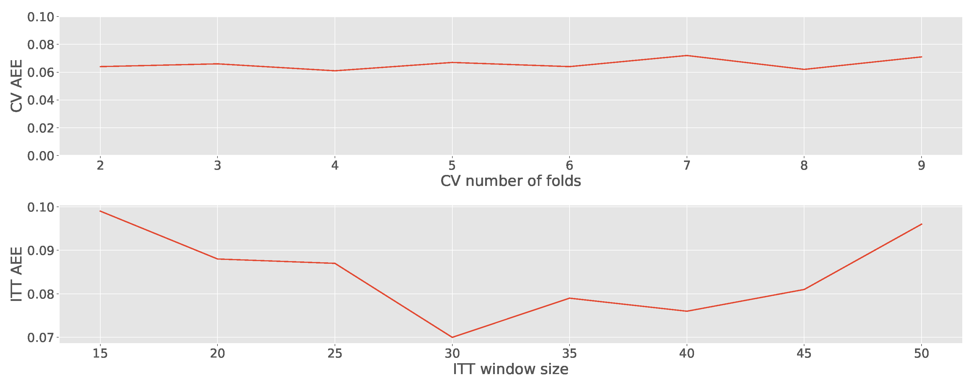
Also, we wanted to analyze parameter choices for the baseline methods. Figure 7 depicts different number of folds for CV and different window sizes for ITT related to their AEE on the OUTDOOR data set for the GLVQ classifier. Changing the number of folds for CV does not seem to have a huge effect in estimating the accuracy. If the ITT window size is too small there can be noise and calculating the average of a smaller window results in coarser granularity. On the other hand, if the window is too big, there is too much delay and information from older states of the classifier has a negative impact. Choosing a window size of 30 seems to be a good trade-off.
Furthermore, we want to analyze different ratios for train/test splits or in other words how many samples training set S and test set S’ contains. For the other experiments, we choose to have a 50/50 split. Figure 8 shows different ratios of the train/test split, again for the GLVQ classifier on the OUTDOOR data set. The results are supporting our findings with the analytical data set from Section 5.2. The AEE remains stable also if the training set S consists of only 10% of the samples from the data set. The error raises to 4%, which is still better than the baseline models, if only 250 samples are in the training set S. However, if the train set is defined too small, CGEM is not capable of building an accurate estimation model.
5.3.3. Active Learning
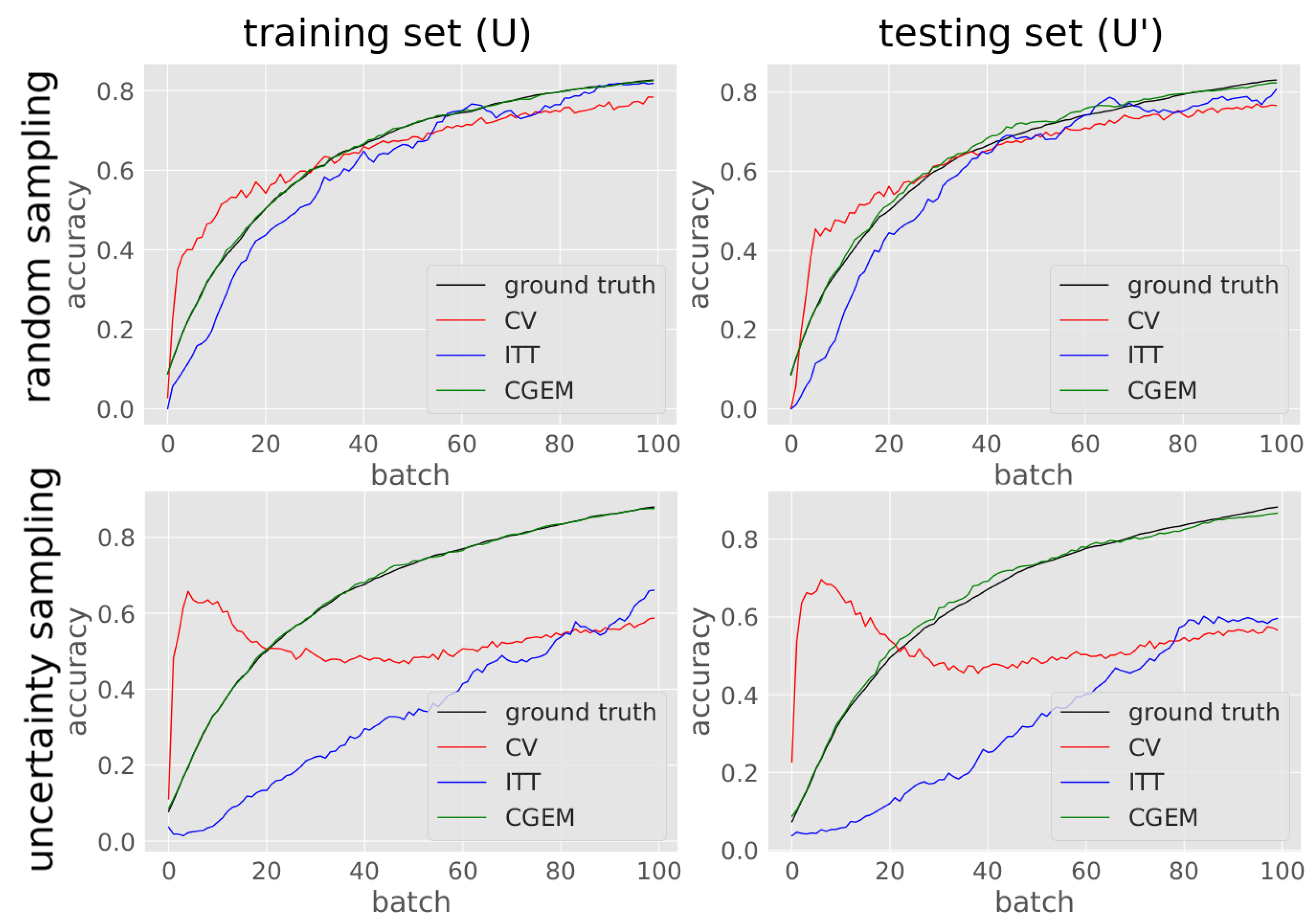
For active learning experiments, uncertainty sampling was used to query the samples with the lowest classifier confidence (see Table 6 and Table 7). The final WCA is usually better compared to random sampling (see Table 5). However, the AEE predicted with CGEM is with 2.3% to 7.2% slightly higher as in the random sampling experiments.
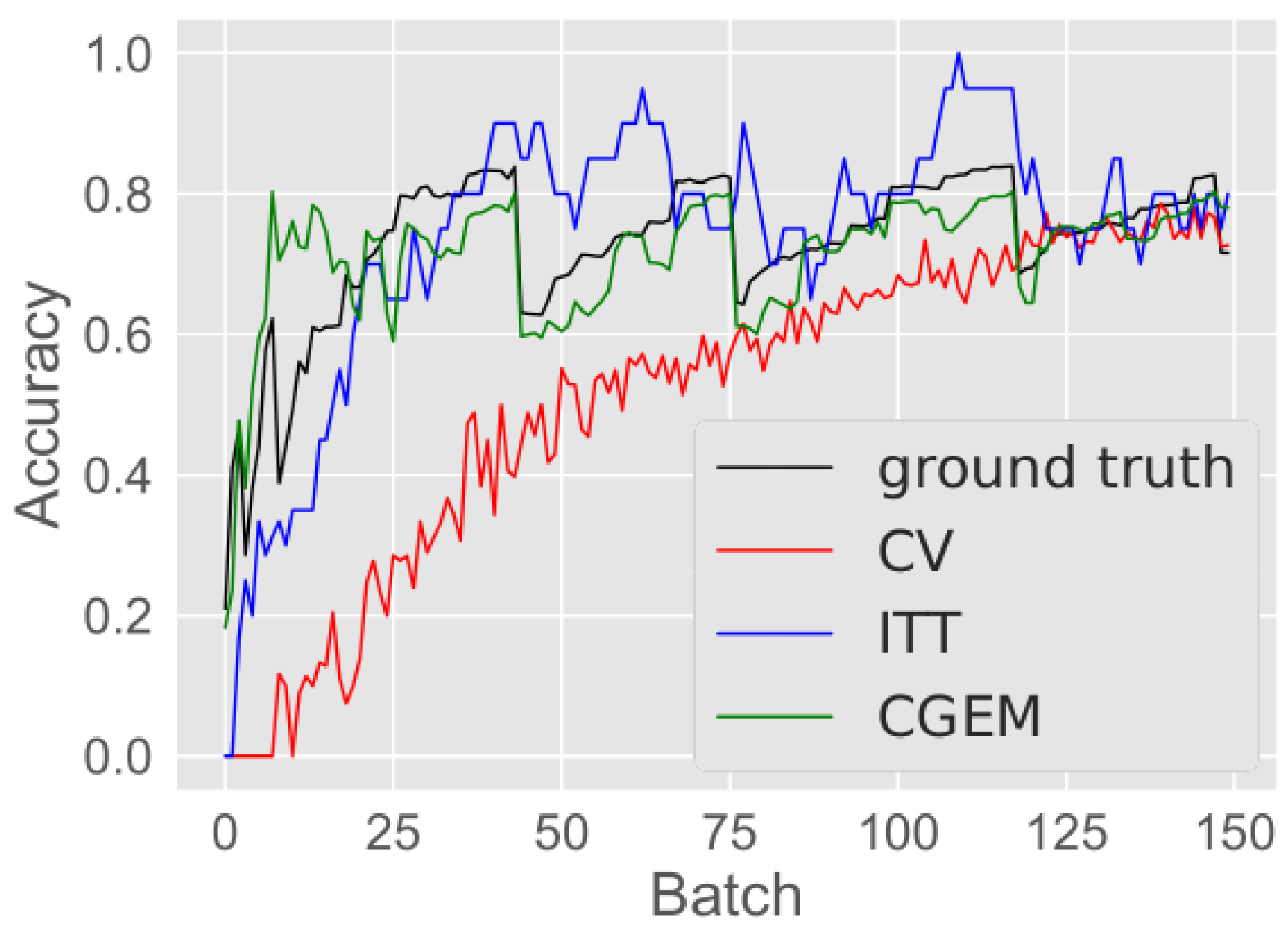
Predicting the accuracy of the classifier when applying an active querying strategy is challenging for the baseline methods, because they are relying on the samples of only and those samples have lowest confidence, meaning they are hard to classify. So, the estimated accuracy is pessimistic in this case. CGEM is adapting to this and still estimates the accuracy with high precision. In Figure 9 averaged incremental training runs are displayed showing the absolute ground-truth and estimated accuracies of training GLVQ on the OUTDOOR data set with both random and active sampling. Figure A2 visualizes the standard deviation of AEE for these trainings.
5.4. Comparison in Resource Demands
CGEM needs to be train beforehand. This requires a labeled data set for extracting configrams to be used to train the regression model. CV and ITT do not need such a preparation phase; however, after training CGEM it can be applied on demand and with no further overhead. Only the regression model must be saved and for estimating the accuracy, confidences of unlabeled samples must be calculated for creating a configram to be fed into CGEM.
ITT is maybe the approach which needs less resources. Memory-wise it is relatively cheap, because only the window of the last classifications must be saved. However, before training any sample, it must be classified because ITT relies on the information whether these classifications were correct or not. This makes ITT relatively inflexible, because these classifications must be done, even if accuracy estimates are not necessary.
CV is the most resource demanding approach. Memory-wise it is expensive because a sufficient number of trained samples must be saved for applying the CV, which is possibly not an option on some mobile robot applications. In our evaluation we saved all yet trained samples for the best possible performance of CV. However, also computation-wise CV is resource demanding, since for estimating the accuracy k classifiers must be trained, where k is the number of CV-folds.
6. Competence-Based Human Machine Interaction
To have a look at a more practical evaluation, we want to know how CGEM can be used as a helper for an efficient human–robot interaction in an more flexible incremental learning setting, where new classes appear while in training. This relates to our use case of a service robot that regularly does a particular job and must adapt to new conditions occasionally. In our training setting, the classifier is not only trained incrementally, but also new samples (including new classes) are inserted to the unlabeled pool U while training. To define the state of sufficient robot capability, a minimum desired task accuracy (MDTA) is defined. If CGEM estimates a lower accuracy than MDTA, the robot stops the task and waits for its supervision. The supervision is done by querying unlabeled samples and asking the user for the respective labels. As in our former evaluation, CGEM is applied after each batch of samples to determine the accuracy increase. This is done until the accuracy is equal to or above the MDTA. If accuracy estimation detects a drop in accuracy again because of newly appearing unknown classes, the robot stops and is retrained until the MDTA is reached again.
To simulate this use case in an experimental setting, the GLVQ classifier is trained on the OUTDOOR data set, which is related to our scenario. We choose GLVQ because it is a very flexible classifier, needs less resources compared to the other evaluated methods and because it is well suited for efficient incremental training [48]. Also, GLVQ performed best on the OUTDOOR data set when using uncertainty sampling and second best when querying randomly.
In our experimental setting the train test split in S and S’ is applied as described earlier. The training of C is commences with only 10 classes from OUTDOOR. The training is done in mini-batches as described earlier. After each mini-batch, the accuracy on is calculated and if it is above an MDTA of 80% the classifier is expected to be good enough until new objects appear. To simulate this, 5 new classes are put in U and continue training until N batches are trained. M is then trained with the extracted configram-accuracy pairs . After that, M is applied to S’ in a similar fashion: is trained as long as its estimated accuracy predicted by CGEM is below 80%. Please note that we do not use ground-truth accuracy data here, but we are capturing it for comparison. Again similar to before, 5 unknown classes are put in if the predicted accuracy is equal or above an MDTA of 80%.
The accuracy plot of can be seen in Figure 10. In the plot the adding of the new samples to is noticeable in a drop of accuracy when the predicted accuracy (green line) is on or above 80%. After the adding, the estimated accuracy is below 0.8 and the classifier is trained again until the MDTA is reached again. Then new samples are added again, the classifier is retrained again and so on. It is visible from the plot that CGEM is also capable of predicting the accuracy in this incremental learning use case, except for some fluctuations in the beginning of training.
7. Conclusions
We showed that the CGEM approach improves the prediction of accuracy for four incremental trained classifiers with their specific confidence estimates. Our analytical experiments show that data distributions need to be similar for training and test conditions, excluding strong drift scenarios. Our in-depth evaluation of several state-of-the-art real-world data sets shows that CGEM estimates the classifier’s accuracy for both random and active learning. Especially for active learning this is crucial, because baseline methods are relying on the labeled training set which is not representative for the whole data distribution. Our CGEM method can resolve this problem by also taking into account the unlabeled data. Further we have shown that CGEM also deals with more interactive learning scenarios where new samples are added while training incrementally.
For using CGEM, it needs to be trained with a labeled training data set first. After being trained once, it can be applied in a very flexible manner and only if needed, without any extra overhead. CGEM also has a very fast reaction time, which is crucial when dealing with fast changing environments as our incremental learning use case has shown. The baseline methods CV and ITT both have a high latency because they are working on a window of trained instances. The main qualitative difference to CV and ITT is the additional exploitation of unlabeled data with respect to the confidences of the targeted classifier.
There is little research done concerning the quality surveillance of continuously learning autonomous intelligent systems. We think that this is an important goal for building adaptive cooperative robots and we hope that a first step towards this was done with this contribution. Further research is needed in analyzing how to apply CGEM to data that is different from the training data and if domain adaptation techniques are applicable here. Also, it would be beneficial to have a confidence for the estimated accuracy to further reject uncertain predictions. For reducing the label effort to create set for training CGEM, it can be explored if data set reduction techniques as described in [14] can be applied, since our experiments show that CGEM is robust in terms of a varying number of samples.
As already motivated in the introduction, a possible application for CGEM could be, e.g., a household service robot. As such a consumer robot is shipped from a factory to a customer it has to learn the individual user environment, where the robot should do a certain task like cleaning the room. The robot is trained incrementally by getting user supervision via a label interface [49] from time to time. In this use case a first simplified goal could be to determine if the accuracy in recognizing key objects in the environment can be estimated if CGEM is pre-trained with other objects within the goal domain. The estimated accuracy could then be used to determine if the robot needs more training or if the user must take a higher workload ratio to accomplish a needed minimal accuracy.
A second goal could be to determine if the estimated accuracy is related to the actual task performance the robot has in its current state (like how good is the robot in cleaning up the environment). Other interesting research within such a real-world application of CGEM could be to determine if the whole task should be delegated, if the performance is not increasing while training. Also, it could be interesting to evaluate a trade-off for training the robot compared to the user is doing the task on his or her own.
Author Contributions
Conceptualization, C.L. and H.W.; Software, C.L.; Supervision, H.W. and H.R.; Writing—original draft, C.L.; Writing—review & editing, H.W. and H.R. All authors have read and agreed to the published version of the manuscript.
Funding
This research received no external funding.
Conflicts of Interest
The authors declare no conflict of interest.
Appendix A
Figure A1.
Configrams of evaluated classifiers extracted at the beginning, middle and end of training. The different kinds of confidence estimations are visible in the configrams, too.
Figure A1.
Configrams of evaluated classifiers extracted at the beginning, middle and end of training. The different kinds of confidence estimations are visible in the configrams, too.

Figure A2.
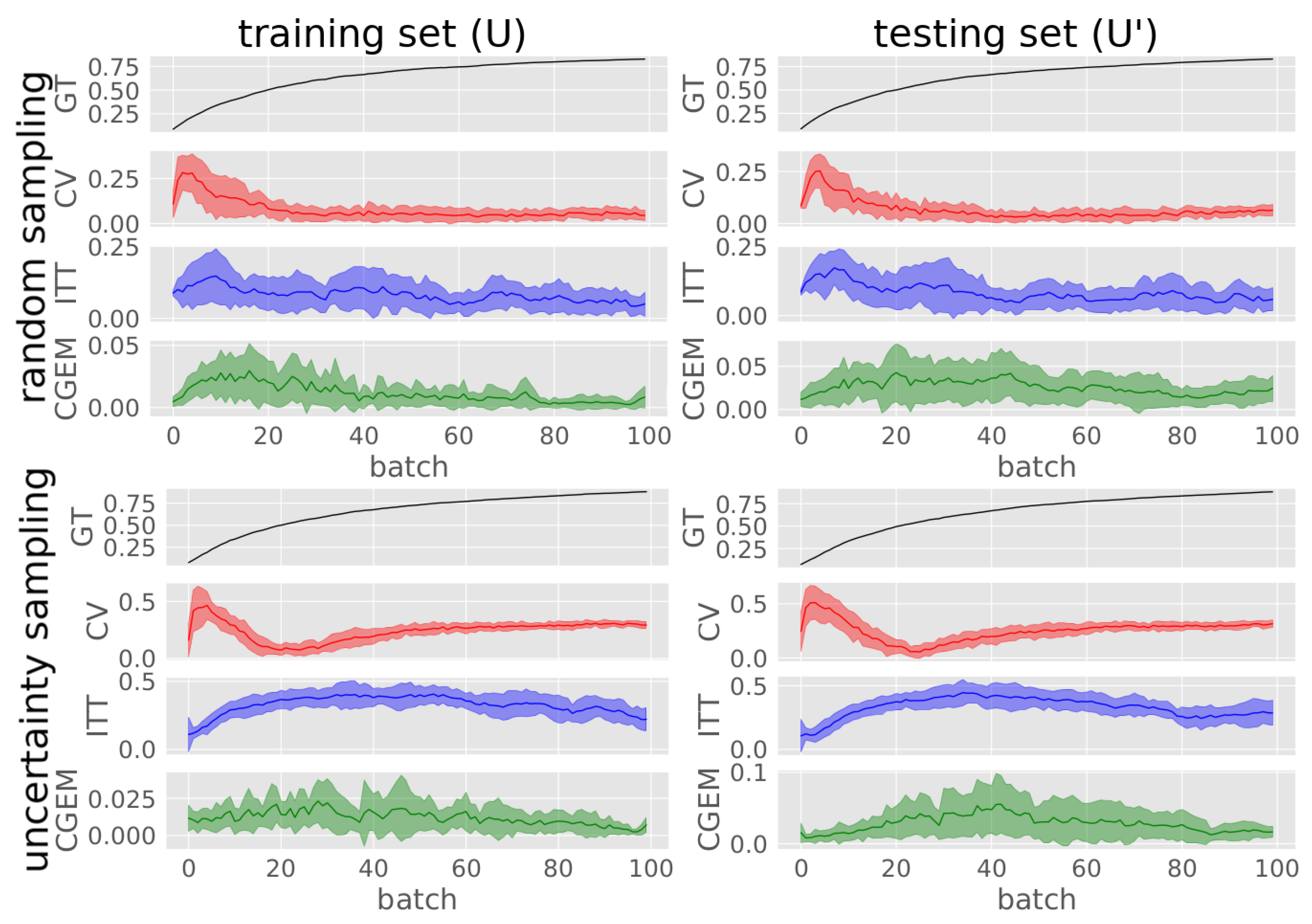
Ground-truth accuracy and accuracy estimation errors with standard deviation of tested approaches for the GLVQ classifier trained on the OUTDOOR data set for both random sampling and uncertainty sampling and both train and test set.
Figure A2.
Ground-truth accuracy and accuracy estimation errors with standard deviation of tested approaches for the GLVQ classifier trained on the OUTDOOR data set for both random sampling and uncertainty sampling and both train and test set.

References
- Wu, B.; Hu, B.; Lin, H. A Learning Based Optimal Human Robot Collaboration with Linear Temporal Logic Constraints. arXiv 2017, arXiv:1706.00007. [Google Scholar]
- Settles, B. Active Learning Literature Survey; Technical Report for University of Wisconsin: Madison, WI, USA, 2010. [Google Scholar]
- Arrieta, A.B.; Díaz-Rodríguez, N.; Del Ser, J.; Bennetot, A.; Tabik, S.; Barbado, A.; García, S.; Gil-López, S.; Molina, D.; Benjamins, R.; et al. Explainable Artificial Intelligence (XAI): Concepts, taxonomies, opportunities and challenges toward responsible AI. Inf. Fusion 2020, 58, 82–115. [Google Scholar] [CrossRef] [Green Version]
- Adadi, A.; Berrada, M. Peeking inside the black-box: A survey on Explainable Artificial Intelligence (XAI). IEEE Access 2018, 6, 52138–52160. [Google Scholar] [CrossRef]
- Roscher, R.; Bohn, B.; Duarte, M.F.; Garcke, J. Explainable machine learning for scientific insights and discoveries. IEEE Access 2020, 8, 42200–42216. [Google Scholar] [CrossRef]
- Gunning, D. Explainable Artificial Intelligence (xai). Available online: https://www.esd.whs.mil/Portals/54/Documents/FOID/Reading%20Room/DARPA/15-F-0059_CLIQR_QUEST_FISCAL_YEAR_2012_RPT.pdf (accessed on 28 August 2020).
- Lundberg, S.M.; Erion, G.; Chen, H.; DeGrave, A.; Prutkin, J.M.; Nair, B.; Katz, R.; Himmelfarb, J.; Bansal, N.; Lee, S.I. From local explanations to global understanding with explainable AI for trees. Nat. Mach. Intell. 2020, 2, 2522–5839. [Google Scholar] [CrossRef] [PubMed]
- Ribeiro, M.T.; Singh, S.; Guestrin, C. “Why should I trust you?” Explaining the predictions of any classifier. In Proceedings of the 22nd ACM SIGKDD International Conference on Knowledge Discovery and Data Mining, San Francisco, CA, USA, 13–17 August 2016; pp. 1135–1144. [Google Scholar]
- Dzindolet, M.T.; Peterson, S.A.; Pomranky, R.A.; Pierce, L.G.; Beck, H.P. The role of trust in automation reliance. Int. J.-Hum.-Comput. Stud. 2003, 58, 697–718. [Google Scholar] [CrossRef]
- Yin, M.; Wortman Vaughan, J.; Wallach, H. Understanding the effect of accuracy on trust in machine learning models. In Proceedings of the 2019 Chi Conference on Human Factors in Computing Systems, Glasgow, UK, 4–9 May 2019; pp. 1–12. [Google Scholar]
- Schmidt, P.; Biessmann, F. Quantifying interpretability and trust in machine learning systems. arXiv 2019, arXiv:1901.08558. [Google Scholar]
- Welinder, P.; Welling, M.; Perona, P. A Lazy Man’s Approach to Benchmarking: Semisupervised Classifier Evaluation and Recalibration. In Proceedings of the IEEE Conference on Computer Vision and Pattern Recognition (CVPR), Portland, OR, USA, 23–28 June 2013; pp. 3262–3269. [Google Scholar]
- Shafer, G.; Vovk, V. A Tutorial on Conformal Prediction. J. Mach. Learn. Res. 2008, 9, 371–421. [Google Scholar]
- Jiang, H.; Kim, B.; Guan, M.; Gupta, M. To trust or not to trust a classifier. In Advances in Neural Information Processing Systems; Neural Information Processing Systems Foundation, Inc. ( NIPS ): London, UK, 2018; pp. 5541–5552. [Google Scholar]
- Platanios, E.; Blum, A.; Mitchell, T. Estimating Accuracy from Unlabeled Data. In Proceedings of the Association for Uncertainty in Artificial Intelligence, UAI, Toronto, ON, Canada, 3–6 August 2014; pp. 682–691. [Google Scholar]
- Donmez, P.; Lebanon, G.; Balasubramanian, K. newblock Unsupervised Supervised Learning I: Estimating Classification and Regression Errors without Labels. JMLR 2010, 11, 1323–1351. [Google Scholar]
- Aghazadeh, O.; Carlsson, S. Properties of Datasets Predict the Performance of Classifiers. In Proceedings of the British Machine Vision Conference, BMVC 2013, Bristol, UK, 9–13 September 2013. [Google Scholar]
- Parisi, G.I.; Kemker, R.; Part, J.L.; Kanan, C.; Wermter, S. Continual lifelong learning with neural networks: A review. Neural Netw. 2019, 113, 54–71. [Google Scholar] [CrossRef]
- Losing, V.; Hammer, B.; Wersing, H. Incremental on-line learning: A review and comparison of state of the art algorithms. Neurocomputing 2018, 275, 1261–1274. [Google Scholar] [CrossRef] [Green Version]
- He, H.; Chen, S.; Li, K.; Xu, X. Incremental Learning From Stream Data. IEEE Trans. Neural Networks 2011, 22, 1901–1914. [Google Scholar]
- Zliobaite, I.; Bifet, A.; Pfahringer, B.; Holmes, G. Active Learning With Drifting Streaming Data. IEEE Trans. Neural Netw. Learn. Syst. 2014, 25, 27–39. [Google Scholar] [CrossRef]
- Lomonaco, V.; Maltoni, D. Core50: A new dataset and benchmark for continuous object recognition. arXiv 2017, arXiv:1705.03550. [Google Scholar]
- Pozzolo, A.D.; Boracchi, G.; Caelen, O.; Alippi, C.; Bontempi, G. Credit Card Fraud Detection: A Realistic Modeling and a Novel Learning Strategy. IEEE Trans. Neural Netw. Learn. Syst. 2018, 29, 3784–3797. [Google Scholar]
- Elwell, R.; Polikar, R. Incremental Learning of Concept Drift in Nonstationary Environments. IEEE Trans. Neural Netw. 2011, 22, 1517–1531. [Google Scholar] [CrossRef] [PubMed]
- Ditzler, G.; Polikar, R. Incremental Learning of Concept Drift from Streaming Imbalanced Data. IEEE Trans. Knowl. Data Eng. 2013, 25, 2283–2301. [Google Scholar] [CrossRef]
- Pesaranghader, A.; Viktor, H.L.; Paquet, E. McDiarmid drift detection methods for evolving data streams. In Proceedings of the 2018 International Joint Conference on Neural Networks (IJCNN), Rio de Janeiro, Brazil, 8–13 July 2018; IEEE: Piscataway, NJ, USA, 2018; pp. 1–9. [Google Scholar]
- Gomes, H.M.; Read, J.; Bifet, A.; Barddal, J.P.; Gama, J. Machine learning for streaming data: State of the art, challenges, and opportunities. ACM SIGKDD Explor. Newsl. 2019, 21, 6–22. [Google Scholar] [CrossRef]
- Ahmad, S.; Lavin, A.; Purdy, S.; Agha, Z. Unsupervised real-time anomaly detection for streaming data. Neurocomputing 2017, 262, 134–147. [Google Scholar] [CrossRef]
- Constantinopoulos, C.; Likas, A. Active Learning with the Probabilistic RBF Classifier. In Proceedings of the International Conference on Artificial Neural Networks (ICANN), Athens, Greece, 10–14 September 2006; pp. 357–366. [Google Scholar]
- Käding, C.; Freytag, A.; Rodner, E.; Bodesheim, P.; Denzler, J. Active learning and discovery of object categories in the presence of unnameable instances. In Proceedings of the Conference on Computer Vision and Pattern Recognition (CVPR), Boston, MA, USA, 7–12 June 2015; pp. 4343–4352. [Google Scholar]
- Seung, S.; Opper, M.; Sompolinsky, H. Query by Committee. In Proceedings of the Fifth Annual Workshop on Computational Learning Theory, Pennsylvania, PA, USA, 27–29 July 1992; pp. 287–294. [Google Scholar]
- Konyushkova, K.; Sznitman, R.; Fua, P. Learning active learning from data. In Proceedings of the Advances in Neural Information Processing Systems, Long Beach, CA, USA, 4–9 December 2017; pp. 4225–4235. [Google Scholar]
- Bachman, P.; Sordoni, A.; Trischler, A. Learning algorithms for active learning. arXiv 2017, arXiv:1708.00088. [Google Scholar]
- Purushotham, S.; Tripathy, B. Evaluation of classifier models using stratified tenfold cross validation techniques. In Proceedings of the International Conference on Computing and Communication Systems, Vellore, India, 9–11 December 2011; Springer: Berlin/Heidelberg, Germany, 2011; pp. 680–690. [Google Scholar]
- Losing, V.; Hammer, B.; Wersing, H. Interactive online learning for obstacle classification on a mobile robot. In Proceedings of the International Joint Conference on Neural Networks (IJCNN), Killarney, Ireland, 12–16 July 2015; pp. 1–8. [Google Scholar]
- Draper, N.R.; Smith, H. Applied Regression Analysis; John Wiley & Sons: Hoboken, NJ, USA, 1998; Volume 326. [Google Scholar]
- Cortes, C.; Vapnik, V. Support-Vector Networks. Mach. Learn. 1995, 20, 273–297. [Google Scholar] [CrossRef]
- Platt, J.C. Probabilistic outputs for support vector machines and comparisons to regularized likelihood methods. Adv. Large Margin Classif. 1999, 10, 61–74. [Google Scholar]
- Breiman, L. Random forests. Mach. Learn. 2001, 45, 5–32. [Google Scholar] [CrossRef] [Green Version]
- Sato, A.; Yamada, K. Generalized Learning Vector Quantization. In Proceedings of the 8th International Conference on Neural Information Processing Systems (NIPS), Denver, CO, USA, 27–30 November 1995; pp. 423–429. [Google Scholar]
- Schleif, F.; Hammer, B.; Villmann, T. Margin-based active learning for LVQ networks. Neurocomputing 2007, 70, 1215–1224. [Google Scholar] [CrossRef]
- Kohonen, T. Improved versions of learning vector quantization. In Proceedings of the IJCNN International Joint Conference on Neural Networks, San Diego, CA, USA, 17–21 June 1990; pp. 545–550. [Google Scholar]
- Street, W.N.; Wolberg, W.H.; Mangasarian, O.L. Nuclear feature extraction for breast tumor diagnosis. Biomedical image processing and biomedical visualization. In Proceedings of the International Society for Optics and Photonics, San Jose, CA, USA, 1–4 February 1993; Volume 1905, pp. 861–870. [Google Scholar]
- Fei-Fei, L.; Fergus, R.; Perona, P. Learning generative visual models from few training examples: An incremental bayesian approach tested on 101 object categories. In Proceedings of the 2004 Conference on Computer Vision and Pattern Recognition Workshop, Washington, DC, USA, 27 June–2 July 2004; IEEE: Piscataway, NJ, USA, 2004; p. 178. [Google Scholar]
- Everingham, M.; Van Gool, L.; Williams, C.K.I.; Winn, J.; Zisserman, A. The PASCAL Visual Object Classes Challenge 2012 (VOC2012) Results. Available online: http://host.robots.ox.ac.uk/pascal/VOC/voc2012/ (accessed on 28 August 2020).
- Simonyan, K.; Zisserman, A. Very Deep Convolutional Networks for Large-Scale Image Recognition. arXiv 2014, arXiv:1409.1556. [Google Scholar]
- Liu, Z.; Luo, P.; Wang, X.; Tang, X. Deep Learning Face Attributes in the Wild. In Proceedings of the International Conference on Computer Vision (ICCV), Santiago, Chile, 7–13 December 2015. [Google Scholar]
- Limberg, C.; Wersing, H.; Ritter, H.J. Efficient accuracy estimation for instance-based incremental active learning. In Proceedings of the European Symposium on Artificial Neural Networks (ESANN), Bruges, Belgium, 25–27 April 2018. [Google Scholar]
- Limberg, C.; Krieger, K.; Wersing, H.; Ritter, H.J. Active Learning for Image Recognition Using a Visualization-Based User Interface. In Proceedings of the International Conference on Artificial Neural Networks (ICANN), Munich, Germany, 17–19 September 2019; pp. 495–506. [Google Scholar]
Figure 1.
Illustration of accuracy estimation. The accuracy estimation model is trained to predict the working classifier accuracy (computed from ground-truth samples) based on confidence histograms (configrams) of the classifier on unlabeled samples.
Figure 1.
Illustration of accuracy estimation. The accuracy estimation model is trained to predict the working classifier accuracy (computed from ground-truth samples) based on confidence histograms (configrams) of the classifier on unlabeled samples.

Figure 2.
A domain D contains data pools . To predict (predictor M) the accuracy of a classifier while incrementally trained on pool (querying labels from , moving samples to , right side), we first create from another instance of the same classifier, but incrementally trained on a “training pool” (with label queries from L, left side), ground-truth data for a regression model M. This regression model captures the relationship between classifier confidences (“configrams”) ϕ and accuracies a on its training pool . Once the model has been formed, it can be used to generalize this relationship to the new pool S’ allowing accurate prediction of the accuracy of incremental training from the unlabeled pool and the few queried labels in . The same model could be used to monitor incremental training on further pools etc. (not depicted).

Figure 3.
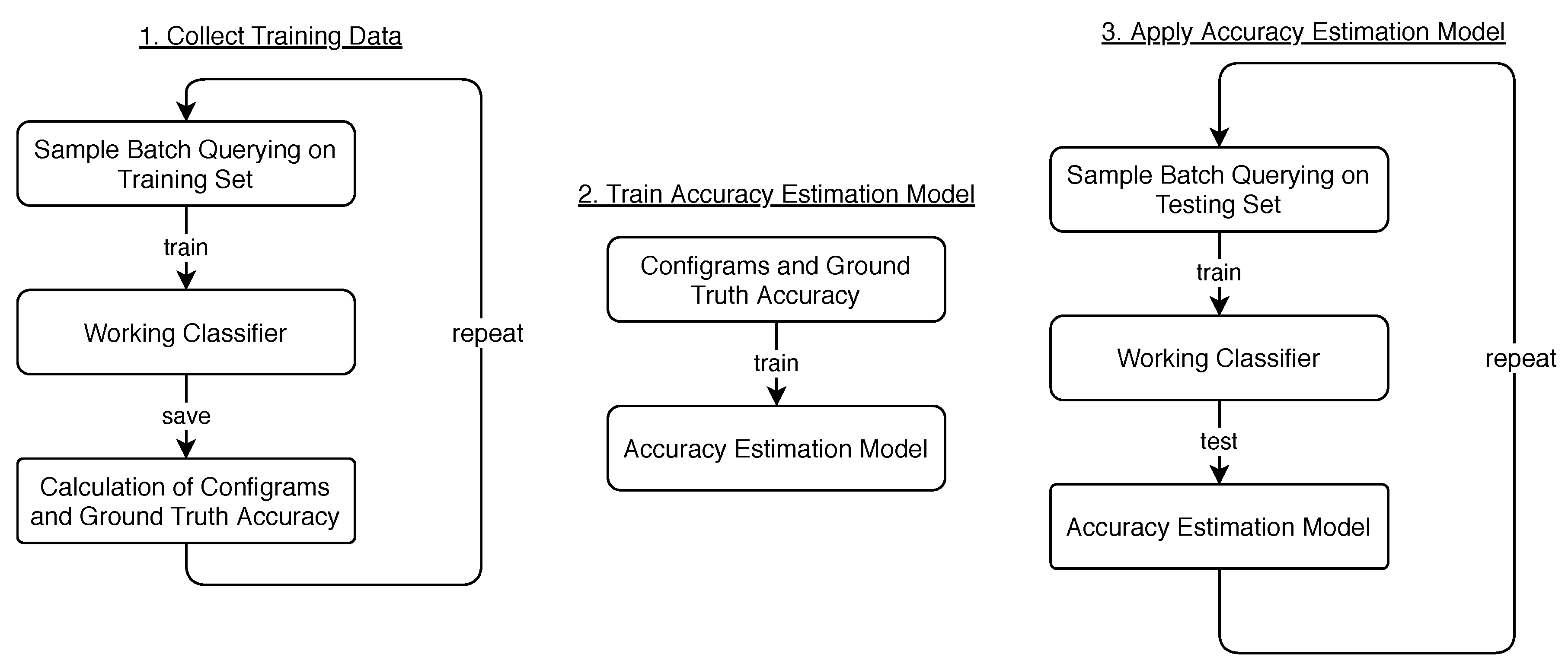
Workflow of accuracy estimation.

Figure 4.
Comparison of regression models used for estimating ground-truth accuracy of several classifiers averaged on tested real-world data sets.
Figure 4.
Comparison of regression models used for estimating ground-truth accuracy of several classifiers averaged on tested real-world data sets.

Figure 5.
Samples drawn from four variants of the Four Gaussian data set. All Gaussians have and their means lie on a circle with radii .
Figure 5.
Samples drawn from four variants of the Four Gaussian data set. All Gaussians have and their means lie on a circle with radii .

Figure 6.
Analytical drifting data sets used for determining properties of CGEM. The base data set is displayed on the top with the six modifications below. Each modification is evaluated in multiple linear intensities, while the figure displays the most intense modification.
Figure 6.
Analytical drifting data sets used for determining properties of CGEM. The base data set is displayed on the top with the six modifications below. Each modification is evaluated in multiple linear intensities, while the figure displays the most intense modification.

Figure 7.
Evaluation of different parameters for cross-validation (CV) and interleaved test/train error (ITT) for GLVQ classifier on the OUTDOOR data set.
Figure 7.
Evaluation of different parameters for cross-validation (CV) and interleaved test/train error (ITT) for GLVQ classifier on the OUTDOOR data set.

Figure 8.
Evaluation of CGEM for different train/test split ratios for GLVQ classifier on OUTDOOR data set (total of 5000 samples).
Figure 8.
Evaluation of CGEM for different train/test split ratios for GLVQ classifier on OUTDOOR data set (total of 5000 samples).

Figure 9.
Ground-truth accuracy and estimated accuracy of the GLVQ classifier trained on the OUTDOOR data set for both random sampling and uncertainty sampling and both train and test set.
Figure 9.
Ground-truth accuracy and estimated accuracy of the GLVQ classifier trained on the OUTDOOR data set for both random sampling and uncertainty sampling and both train and test set.

Figure 10.
CGEM applied in one incremental learning use case where new classes are added to the unlabeled pool while training (noticeable in the decays of accuracy). CGEM, ITT and CV are used to estimate the ground-truth accuracy. New samples are added to the unlabeled pool, when the estimated accuracy by CGEM is over 80%.


Table 1.
Working Classifier Accuracies (WCA) after training on Four Gaussians data sets r1, r2, r3, r4.
Table 1.
Working Classifier Accuracies (WCA) after training on Four Gaussians data sets r1, r2, r3, r4.
| r4 | r3 | r2 | r1 | |
|---|---|---|---|---|
| OBC | 0.996 | 0.962 | 0.853 | 0.564 |
| GLVQ | 0.993 | 0.946 | 0.813 | 0.527 |
| KNN | 0.994 | 0.953 | 0.813 | 0.477 |
| RFC | 0.983 | 0.941 | 0.809 | 0.49 |
| SVM | 0.993 | 0.956 | 0.838 | 0.556 |
Table 2.
Accuracy Estimation Errors (AEE) of tested classifiers on Four Gaussians data sets.
| r4 | r3 | r2 | r1 | Average | ||
|---|---|---|---|---|---|---|
| GLVQ | CV | 0.028 | 0.042 | 0.057 | 0.07 | 0.049 |
| ITT | 0.066 | 0.088 | 0.11 | 0.107 | 0.093 | |
| CGEM | 0.005 | 0.013 | 0.031 | 0.039 | 0.022 | |
| KNN | CV | 0.036 | 0.048 | 0.064 | 0.071 | 0.055 |
| ITT | 0.071 | 0.088 | 0.105 | 0.102 | 0.091 | |
| CGEM | 0.012 | 0.019 | 0.026 | 0.027 | 0.021 | |
| RFC | CV | 0.035 | 0.046 | 0.066 | 0.071 | 0.055 |
| ITT | 0.081 | 0.094 | 0.104 | 0.101 | 0.095 | |
| CGEM | 0.02 | 0.024 | 0.03 | 0.029 | 0.026 | |
| SVM | CV | 0.034 | 0.046 | 0.062 | 0.071 | 0.053 |
| ITT | 0.067 | 0.086 | 0.106 | 0.105 | 0.091 | |
| CGEM | 0.015 | 0.019 | 0.021 | 0.025 | 0.02 |
Table 3.
Evaluation of the accuracy estimation error while applying CGEM to drifting data. Each drifting modifications to the base data set is evaluated in different linear intensities, where 6 the modification that most drifted away from training data.
Table 3.
Evaluation of the accuracy estimation error while applying CGEM to drifting data. Each drifting modifications to the base data set is evaluated in different linear intensities, where 6 the modification that most drifted away from training data.
| 1 | 2 | 3 | 4 | 5 | 6 | |
|---|---|---|---|---|---|---|
| size both | 0.015 | 0.018 | 0.021 | 0.023 | 0.028 | 0.031 |
| size one | 0.015 | 0.017 | 0.017 | 0.018 | 0.019 | 0.02 |
| samples both | 0.018 | 0.015 | 0.015 | 0.015 | 0.014 | 0.014 |
| samples one | 0.022 | 0.025 | 0.023 | 0.035 | 0.028 | 0.027 |
| move | 0.165 | 0.281 | 0.089 | 0.04 | 0.278 | 0.347 |
| squeeze | 0.021 | 0.032 | 0.039 | 0.042 | 0.054 | 0.068 |
Table 4.
Evaluation of accuracy estimation error (AEE) of CGEM approach compared to baseline models. The classifier was trained incrementally with random sampling. Accuracy estimation was done after each batch. The table shows mean absolute error (MAE) compared to ground truth.
Table 4.
Evaluation of accuracy estimation error (AEE) of CGEM approach compared to baseline models. The classifier was trained incrementally with random sampling. Accuracy estimation was done after each batch. The table shows mean absolute error (MAE) compared to ground truth.
| WDBC | CALTECH | PASCALVOC2012 | OUTDOOR | CELEBA | Average | ||
|---|---|---|---|---|---|---|---|
| GLVQ | CV | 0.059 | 0.07 | 0.05 | 0.067 | 0.04 | 0.057 |
| ITT | 0.075 | 0.07 | 0.072 | 0.083 | 0.066 | 0.073 | |
| CGEM | 0.052 | 0.025 | 0.033 | 0.026 | 0.016 | 0.03 | |
| KNN | CV | 0.035 | 0.065 | 0.056 | 0.096 | 0.029 | 0.056 |
| ITT | 0.064 | 0.075 | 0.079 | 0.078 | 0.052 | 0.07 | |
| CGEM | 0.039 | 0.041 | 0.044 | 0.058 | 0.018 | 0.04 | |
| RFC | CV | 0.033 | 0.047 | 0.038 | 0.086 | 0.024 | 0.046 |
| ITT | 0.051 | 0.067 | 0.066 | 0.075 | 0.045 | 0.061 | |
| CGEM | 0.022 | 0.031 | 0.016 | 0.031 | 0.015 | 0.023 | |
| SVM | CV | 0.049 | 0.072 | 0.047 | 0.073 | 0.021 | 0.052 |
| ITT | 0.082 | 0.079 | 0.071 | 0.079 | 0.046 | 0.071 | |
| CGEM | 0.066 | 0.04 | 0.024 | 0.041 | 0.015 | 0.037 |
Table 5.
Final classifier accuracies of real-world random sampling experiments.
| WDBC | CALTECH | PASCALVOC2012 | OUTDOOR | CELEBA | |
|---|---|---|---|---|---|
| GLVQ | 0.765 | 0.621 | 0.442 | 0.83 | 0.816 |
| KNN | 0.919 | 0.498 | 0.454 | 0.683 | 0.981 |
| RFC | 0.953 | 0.329 | 0.273 | 0.544 | 0.976 |
| SVM | 0.859 | 0.65 | 0.494 | 0.857 | 0.986 |
Table 6.
Evaluation of accuracy estimation error (AEE) of CGEM approach compared to baseline models. The classifier was trained with incrementally using Active Learning with an uncertainty sampling querying strategy. Accuracy estimation was done after each batch. The table shows mean absolute error (MAE) compared to ground truth.
| WDBC | CALTECH | PASCALVOC2012 | OUTDOOR | CELEBA | Average | ||
|---|---|---|---|---|---|---|---|
| GLVQ | CV | 0.189 | 0.182 | 0.082 | 0.255 | 0.13 | 0.168 |
| ITT | 0.186 | 0.31 | 0.165 | 0.331 | 0.386 | 0.276 | |
| CGEM | 0.056 | 0.052 | 0.045 | 0.028 | 0.013 | 0.039 | |
| KNN | CV | 0.128 | 0.225 | 0.127 | 0.21 | 0.251 | 0.188 |
| ITT | 0.124 | 0.257 | 0.239 | 0.319 | 0.463 | 0.28 | |
| CGEM | 0.021 | 0.1 | 0.049 | 0.095 | 0.014 | 0.056 | |
| RFC | CV | 0.122 | 0.145 | 0.096 | 0.207 | 0.19 | 0.152 |
| ITT | 0.098 | 0.217 | 0.148 | 0.281 | 0.442 | 0.237 | |
| CGEM | 0.008 | 0.035 | 0.029 | 0.031 | 0.014 | 0.023 | |
| SVM | CV | 0.204 | 0.39 | 0.137 | 0.333 | 0.311 | 0.275 |
| ITT | 0.184 | 0.235 | 0.191 | 0.208 | 0.397 | 0.243 | |
| CGEM | 0.131 | 0.075 | 0.059 | 0.063 | 0.035 | 0.072 |
Table 7.
Final classifier accuracies of real-world uncertainty sampling experiments.
| WDBC | CALTECH | PASCALVOC2012 | OUTDOOR | CELEBA | |
|---|---|---|---|---|---|
| GLVQ | 0.991 | 0.571 | 0.413 | 0.882 | 0.869 |
| KNN | 1.0 | 0.51 | 0.469 | 0.715 | 0.967 |
| RFC | 1.0 | 0.346 | 0.338 | 0.664 | 0.979 |
| SVM | 1.0 | 0.472 | 0.51 | 0.811 | 0.97 |
© 2020 by the authors. Licensee MDPI, Basel, Switzerland. This article is an open access article distributed under the terms and conditions of the Creative Commons Attribution (CC BY) license (http://creativecommons.org/licenses/by/4.0/).
Share and Cite
MDPI and ACS Style
Limberg, C.; Wersing, H.; Ritter, H. Beyond Cross-Validation—Accuracy Estimation for Incremental and Active Learning Models. Mach. Learn. Knowl. Extr. 2020, 2, 327-346. https://0-doi-org.brum.beds.ac.uk/10.3390/make2030018
AMA Style
Limberg C, Wersing H, Ritter H. Beyond Cross-Validation—Accuracy Estimation for Incremental and Active Learning Models. Machine Learning and Knowledge Extraction. 2020; 2(3):327-346. https://0-doi-org.brum.beds.ac.uk/10.3390/make2030018
Chicago/Turabian StyleLimberg, Christian, Heiko Wersing, and Helge Ritter. 2020. "Beyond Cross-Validation—Accuracy Estimation for Incremental and Active Learning Models" Machine Learning and Knowledge Extraction 2, no. 3: 327-346. https://0-doi-org.brum.beds.ac.uk/10.3390/make2030018