
Estimating Neural Network’s Performance with Bootstrap: A Tutorial


1
TOELT LLC, Birchlenstr. 25, 8600 Dübendorf, Switzerland
2
School of Computing, University of Portsmouth, Portsmouth PO1 3HE, UK
3
Institute of Applied Mathematics and Physics, Zurich University of Applied Sciences, Technikumstrasse 9, 8401 Winterthur, Switzerland
*
Author to whom correspondence should be addressed.
Mach. Learn. Knowl. Extr. 2021, 3(2), 357-373; https://0-doi-org.brum.beds.ac.uk/10.3390/make3020018
Submission received: 20 January 2021
/
Revised: 23 March 2021
/
Accepted: 25 March 2021
/
Published: 29 March 2021
(This article belongs to the Section Network)
Abstract
:Neural networks present characteristics where the results are strongly dependent on the training data, the weight initialisation, and the hyperparameters chosen. The determination of the distribution of a statistical estimator, as the Mean Squared Error (MSE) or the accuracy, is fundamental to evaluate the performance of a neural network model (NNM). For many machine learning models, as linear regression, it is possible to analytically obtain information as variance or confidence intervals on the results. Neural networks present the difficulty of not being analytically tractable due to their complexity. Therefore, it is impossible to easily estimate distributions of statistical estimators. When estimating the global performance of an NNM by estimating the MSE in a regression problem, for example, it is important to know the variance of the MSE. Bootstrap is one of the most important resampling techniques to estimate averages and variances, between other properties, of statistical estimators. In this tutorial, the application of resampling techniques (including bootstrap) to the evaluation of neural networks’ performance is explained from both a theoretical and practical point of view. The pseudo-code of the algorithms is provided to facilitate their implementation. Computational aspects, as the training time, are discussed, since resampling techniques always require simulations to be run many thousands of times and, therefore, are computationally intensive. A specific version of the bootstrap algorithm is presented that allows the estimation of the distribution of a statistical estimator when dealing with an NNM in a computationally effective way. Finally, algorithms are compared on both synthetically generated and real data to demonstrate their performance.
1. Introduction
An essential step in the design of a neural network model (NNM) is the definition of the neural network architecture [1]. In this tutorial, the analysis assumes that the network architecture design phase is completed and the parameters not varied anymore. It is assumed that a dataset S is available. For the training and testing of an NNM, S is split into two parts, and called the training dataset () and validation dataset (), with and . The model is then trained on . Afterwards, a given statistical estimator, , is evaluated on both and (indicated with and ) to check for overfitting [1]. can be, for example, the accuracy in a classification problem, or the Mean Square Error (MSE) in a regression one. is clearly dependent (sometimes strongly) on both and , as the NNM was trained on . The metric evaluated on the validation dataset may be indicated as
to make its dependence on the two datasets and transparent. The difficulty in evaluating the distributions of is that it is enough to split the data differently (or in other words, to get different and ), for the metric to assume a different value. This poses the question on how to evaluate the performance of an NNM.
One of the most important characteristics of an NNM is its ability to generalise to unseen data, or to maintain its performance when applied to any new dataset. If a model can predict a quantity with an accuracy of, for example, 80%, the accuracy should remain around 80% when the model is applied to new and unseen data. However, changing the training data will change the performance of any given NNM. To give an example of why giving one single number to measure the performance of a NNM can be misleading, let us consider the following example. Suppose we are dealing with a dataset where one of the features is the age. What would happen if, for sheer bad luck, one splits the dataset in one () with only young people, and one () with only old people? The trained NNM will, of course, not be able to generalize well to age groups that are different from those present in . Therefore, the model performance, measured by the the statistical estimator , will drop significantly. This problem can only be identified by considering multiple splits and by studying the distribution of .
The only possibility to estimate the variance of the performance of the model given a dataset S is to split S in many different ways (and, therefore, obtain many different training and validation datasets). Then, the NNM has to be trained on each training dataset. Finally, the chosen statistical estimator can be evaluated on the respective validation datasets. This will allow to calculate the average and variance of , and use these values as an estimate of the performance of the NNM when applied to different datasets. This technique will be called the “split/train algorithm” in this tutorial. The major disadvantage of this technique is that it requires to repeat the training of the NNM for every split, and is therefore very time-consuming. If the model is large, it will require an enormous amount of computing time, making it not always a practical approach.
This paper shows how this difficulty can be overcome using resampling techniques to give an estimate of the average and the variance of metrics as the MSE or the accuracy, thus avoiding the training of hundreds or thousands of models. An alternative to resampling techniques are so-called ensemble methods, namely, algorithms that train a set of models and then generate a prediction by taking a combination of each single prediction. The interested reader is referred to [2,3,4,5,6,7,8,9].
The goal of this tutorial is to present the main resampling methods, and discuss their applications and limitations when used with NNMs. With the information contained in this tutorial, a reader with some experience in programming should be able to implement them. This tutorial is not meant to be an exhaustive review of the mentioned algorithms. The interested reader is referred to the extensive list of references given in each section for a discussion of the theoretical limitations.
The main contributions of this tutorial are four. Firstly, it highlights the role of the Central Limit Theorem (CLT) in describing the distribution of averaging statistical estimators, like the MSE, in the context of NNMs. Particularly in this work, it is shown how the distribution of, for example, the MSE will tend to a normal distribution for increasing sample size, thus justifying the use of the average and the standard deviation to describe it. Secondly, it provides a short review of the main resampling techniques (hold-out set approach, leave-one-out cross-validation, k-fold cross-validation, jackknife, subsampling, split/train, bootstrap) with an emphasis on the challenges when using neural networks. For most of the above-mentioned techniques, the steps are described with the help of a pseudo-code to facilitate the implementation. Thirdly, bootstrap, split/train, and the mixed approach between bootstrap and split/train are discussed in more depth, again with the help of the pseudo-code, including the application to synthetic and real datasets. Finally, limitations and promising future research directions in this area are briefly discussed. Details of implementations of resampling techniques on the problem of high complexity goes beyond the scope of this work, and the reader is referred to the following examples [10,11,12].
This tutorial is structured in the following way. In Section 2 the notation is explained, followed by a discussion of the CLT and its relevance for NNMs in Section 3. A short introduction to the idea behind bootstrap is presented in Section 4, while other resampling algorithms are discussed in Section 5. In Section 6, bootstrap, split/train, and the mixed approach between bootstrap and split/train are explained in more detail, and compared. Practical examples with both synthetic and real data are described in Section 7 and Section 8, respectively. Finally, an outlook and the conclusions are presented in Section 9 and Section 10, respectively.
2. Notation
n independent, identically distributed (iid) observations will be indicated here with . This dataset will come from a population described by a probability density function (PDF) F generally unknown:
Let us assume that the statistical estimator (for example, the average or the mean squared error) is a functional. Loosely speaking, will be a mapping from the space of possible PDFs into real numbers . To make the concept clear, let’s suppose that the estimator is the mean of the observations . In this case,
where it is clear that the right part of Equation (3) is a real number. Unfortunately, in all practical cases, the “real” PDF F is unknown. Given a certain dataset , the only possibility is to approximate the estimator with , where indicates the empirical distribution obtained from by giving a probability of to each observation . This is the idea at the basis of the bootstrap algorithm, as it will be discussed in detail in Section 4.
3. Central Limit Theorem for an Averaging Estimator
A lot of mathematics has been developed to get at least the asymptotic distribution of for [13,14,15,16]. The CLT [17], also known as the Lindeberg–Lévy central limit theorem, enunciates that, considering a sequence of iid observations with (the expected value of the inputs), and , then
where
For any practical purpose, if n is large enough, the normal distribution will give a good approximation of the distribution of the average of a dataset of n iid observations, .
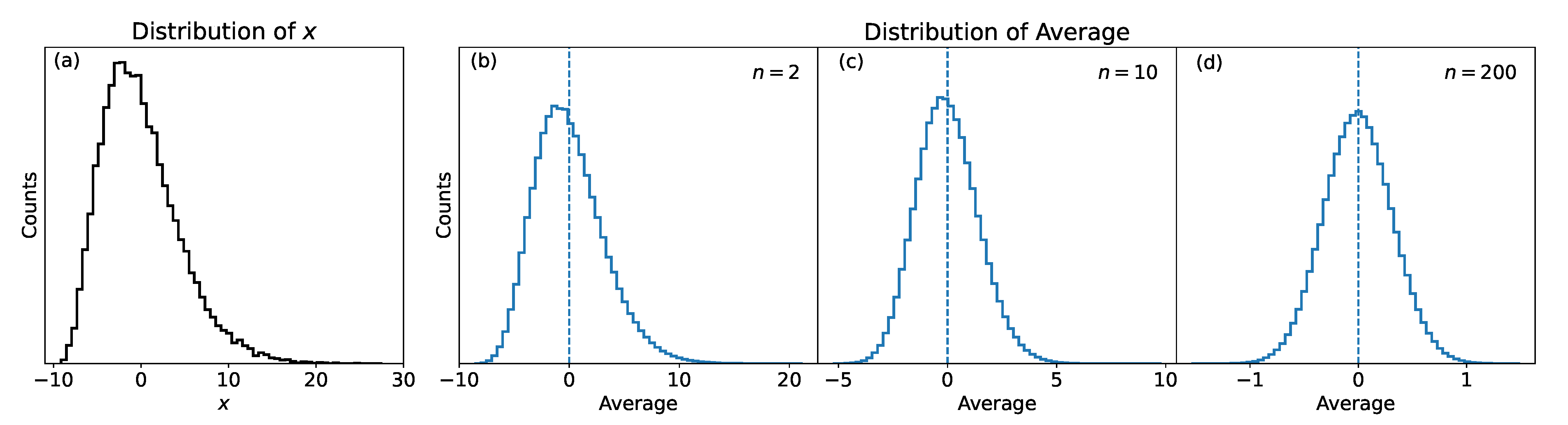
Let’s consider F to be a chi-squared distribution (notoriously asymmetric) with [18] normalized to have the average equal to zero (panel(a) in Figure 1). Let’s now calculate the average of , as in Equation (5) 10 times in three cases: n = 2, 10, 200. The results are shown in Figure 1, panels (b) to (d). When the sample size is small (, panel(b)), the distribution is clearly not symmetrical, but when the sample size grows (panels (c) and (d)), the distribution approximates the normal distribution. Figure 1 is a numerical demonstration of the CLT.
Typically, when dealing with neural networks both in regression and classification problems, one has to deal with complicated functions like the MSE, the cross-entropy, accuracy, or other metrics [1]. Therefore, it may seem that the central limit theorem does not play a role in any practical application involving NNMs. This, however, is not true. Consider, as an example, the MSE function of a given dataset of input observations with average
It is immediately evident that Equation (6) is nothing other than the average of the transformed inputs . Note that the CLT does not make any assumption on the distribution of the observations. Thus, the CLT is also valid for the average of observations that have been transformed (as long as the average and variance of the transformed observations remain finite). In other words, it is valid for both and . This can be formalized in the following Corollaries.
Corollary 1.
Given a dataset of i.i.d. observations with a finite mean μ and variance , define the quantities . The limiting form of the distributions of the MSE (the average of the )
for will be the normal distribution
where with and , we have indicated the expected value and the standard deviation of the , respectively.
Proof.
The first thing to note is that since the have finite mean and finite variance, it follows that will also have finite mean and finite variance, and therefore the CLT can be applied to the average of the . By applying the CLT to the quantities , Equation (8) is obtained. That concludes the proof. □
A numerical demonstration of this result can be clearly seen in Section 7.1. In particular, Figure 2 shows that the distribution of the MSEs approximates when the sample size is large enough.
Note that Corollary 1 can be easily generalized to any estimator in the form
if the quantities have a finite mean and variance . For completeness, the Corollary 1 can be written in the general form.
Corollary 2.
Given a dataset of i.i.d. observations with a finite mean μ and variance , we define the quantities . It is assumed that the average and the variance are finite. The limiting form of the distributions of the estimator θ
for will be the normal distribution
Proof.
The proof is trivial, as it is simply necessary to apply the central limit theorem to the quantities since the is nothing other than the average of those quantities. □
The previous corollaries play a major role for neural networks. The implications of the final distributions of averaging metrics being Gaussian are that:
- The distribution is symmetric around the average, with the same number of observations below and above it; and
- The standard deviation of the distribution can be used as a statistical error, knowing that ca. 68% of the results will be in a region of around the average.
These results justify the use of the average of the statistical estimator, such as the MSE, and of its standard deviation as the only parameters needed to describe the network performance.
4. Bootstrap
Bootstrap is essentially a resampling algorithm. It was introduced by Efron in 1979 [19], and it offers a simulation-based approach for estimating, for example, the variance of statistical estimates of a random variable. It can be used in both parametric and non-parametric settings. The main idea is quite simple and consists of creating new datasets from an existing one by resampling with repetition. The discussion here is limited to the case of n observations that are iid (see Section 2 for more details). The estimator calculated on the simulated datasets will then approximate the estimator evaluated on the true population, which is unknown.
There has been a huge amount of work done on the use of bootstrap and its theoretical limitations. The interested reader is referred to several general overviews [20,21,22,23,24,25,26,27,28,29,30,31,32], to the discussion on the evaluation of the confidence intervals [26,27,29,33,34], to the discussion on how to remove the iid hypothesis [26,35], and the application and limitations in various fields, from medicine to nuclear physics and geochemistry [5,26,27,28,29,36,37,38,39,40,41]. An analysis of the statistical theory on which the bootstrap method is based, goes beyond this tutorial and will not be covered here.
The best way to understand the bootstrap technique is to describe it in pseudo-code, as this illustrates its steps. The original bootstrap algorithm proposed by Efron [19], can be seen in pseudo-code in Algorithm 1. In the Algorithm, is an integer and indicates the number of new samples generated with the bootstrap algorithm.
| Algorithm 1: Pseudo-code of the bootstrap algorithm. |
 |
As a consequence of Corollary 2 (Section 3), Algorithm 1 for a large enough gives an approximation of the average and variance of the statistical estimator . Being the Gaussian distribution (albeit for ), these two parameters describe it completely.
An important question is how big should be. In the original article, Efron [42] suggests that of the order of 100 is already enough to get reasonable estimates. Chernick [26] considers already very large and more than enough. In the latter work, however, it is indicated that, above a certain value of , the error is due to the approximation of the true distribution F by the empirical distribution , rather than by the low number of samples. Therefore, particularly given the computational power available today, it is not meaningful to argue whether 100 or 500 is enough, as running the algorithm with many thousands of samples will take only a few minutes on most modern computers. In many practical applications, using between 5000 and 10,000 is commonplace [26]. As a general rule of thumb, is large enough when the distribution of the estimator starts to resemble a normal distribution.
The method described here is very advantageous when using neural networks because it allows an estimation of average and variance of quantities as the MSE or the accuracy without training the model hundreds or thousands of times, as will be described in Section 6. Thus, it is extremely attractive from a computational point of view and is a very pragmatic solution to a potentially very time-consuming problem. The specific details and pseudo-code of how to apply this method to NNMs will be discussed at length in Section 6.
5. Other Resampling Techniques
For completeness, in this section, additional techniques—namely the hold-out set approach, leave-one-out cross-validation, k-fold cross-validation, jackknife, and subsampling—are briefly discussed, including their limitations. For an in-depth analysis, the interested reader is referred to [43] and to the given literature.
5.1. Hold-Out Set Approach
The simplest approach to estimating a statistical estimator is to randomly divide the dataset into two parts: a training and a validation dataset . The validation dataset is sometimes called a hold-out set (from which derives the name of this technique). The model is trained on the training dataset , and then used to evaluate on the validation dataset . is used as an estimate of the expected value of . This approach is also used to identify whether the model overfits, or, in other words, learns to unknowingly extract some of the noise in the data as if that would represent an underlying model structure [1]. The presence of overfitting is checked by comparing and . A large difference is an indication that overfitting is present. The interested reader can find a detailed discussion in [1]. Such an approach is widely used, but has two major drawbacks [43]. Firstly, since the split is done only once, it can happen that is not representative of the entire dataset, as described in the age example in Section 1. Using this approach would not allow for an identification of such a problem, therefore giving the impression that the model has very bad performance. In other words, this method is highly dependent on the dataset split. The second drawback is that splitting the dataset will reduce the number of observations available in the training dataset, therefore making the training of the model less effective.
The techniques explained in the following sections try to address these two drawbacks with different strategies.
5.2. Leave-One-Out Cross-Validation
Leave-one-out cross-validation (LOOCV) can be well-understood with the pseudo-code outlined in Algorithm 2.
| Algorithm 2: Leave-one-out cross-validation (LOOCV) algorithm. |
 |
This approach has the clear advantage that the model is trained on almost all observations. Therefore, we address the second drawback of the hold-out approach, namely that there are less observations for training. This also has the consequence that the LOOCV tends not to overestimate the estimate of the statistical estimator [43] as much as the hold-out approach. The second major advantage is that this approach will not present the problem that was described in the age example in the introduction as the training dataset will include almost all observations, and it will vary n times.
The approach, however, has one major drawback: it is very computationally expensive to implement, if the NNM training is resource-intensive. In all medium to large NNM models, this approach is simply not a realistic possibility.
5.3. k-Fold Cross-Validation
k-fold cross-validation (k-fold CV) is similar to LOOCV but tries to address the drawback that the model has to be trained n times. The method involves randomly dividing the dataset in k groups (also called folds) of approximately equal size. The method is outlined in pseudo-code in Algorithm 3.
| Algorithm 3: k-fold cross-validation (k-fold CV) algorithm. |
 |
Therefore, LOOCV is simply a special case of k-fold CV for . Typical k values are 5 to 10. The main advantage of this method with respect to LOOCV is clearly computational. The model has to be trained only k times instead of n.
When the dataset is not big, k-fold CV has the drawback that it reduces the number of observations available for training and for estimating , since each fold will be k times smaller than the original dataset. Additionally, it may be argued that using only a few values of the statistical estimator (for example, 5 or 10) to study its distribution is questionable [43].
5.4. Jackknife
The jackknife algorithm [44,45] is another resampling technique that was first developed by Quenouille [44] in 1949. It consists of creating n samples by simply removing one observation each time from the available . For example, one jackknife sample will be , with elements. To estimate , the statistical estimator will be evaluated on each sample (of size ). Note that the jackknife may seem to be the exact same method as LOOCV, but there is one major difference that is important to highlight. While in LOOCV, is evaluated on the observation held out (in other words, on one single observation), in jackknife, is evaluated on the remaining observations.
With this method, it is only possible to generate n samples that can then be used to evaluate an approximation of a statistical estimator. This is one significant limitation of the method compared to bootstrap. If the size of the dataset is small, only a limited number of samples will be available. The interested reader is referred to the reviews [28,29,46,47,48,49,50]. A second major limitation is that the jackknife estimation of an averaging estimator coincides with the average and standard deviation of the observations [26]. Thus, using jackknife is not helpful to approximate .
For the limitations discussed above, this technique is not particularly advantageous when dealing with NNMs, and therefore, is seldom used in such a context, especially when compared with the bootstrap algorithm and its advantages.
5.5. Subsampling
Another technique for resampling is subsampling, achieved by simply choosing from a dataset with n elements, elements without replacement. As a result, the samples generated with this algorithm have a smaller size than the initial dataset . As the bootstrap algorithm, this one has been widely studied and used in the most different fields, from genomics [51,52] to survey science [53,54], finance [55,56] and, of course, statistics [26,57,58]. The two reviews [26,59] can be consulted by the interested reader. Precise conditions under which approximating with subsampling lead to a good approximation of the desired estimator can be found in [59,60,61,62].
Subsampling presents a fundamental difficulty when dealing with the average as a statistical estimator. By its own nature, subsampling requires to consider a sample of smaller size m than the available dataset (of size n). As seen previously, the CLT enunciates that the standard deviation of a sample of size m will tend asymptotically to a normal distribution with a standard deviation that is proportional to the inverse of . That means that changing the sample size changes the standard deviation of the distribution of . Note that this is not a reflection of properties of the MSE, but only of the sample chosen. In the extreme case that (one could argue that this is not subsampling anymore, but let’s consider it as an extreme case) the average estimator will always have the same value, exactly the average of the inputs, since the subsampling samples are without replacement, and therefore the standard deviation will be zero. On the other hand, if , the standard deviation will increase significantly and will coincide with the standard deviation of the observations.
Therefore, the subsampling method presents the fundamental problem of the choice of m. Since there is not a general criterion to choose m, the distribution of will reflect the arbitrary choice of m and the properties of the data at the same time. This is why the authors do not think that the subsampling method is well-suited to give a reasonable and interpretable estimate of the distribution of a statistical estimator, as the MSE.
6. Algorithms for Performance Estimation
As discussed in Section 1, the performance of an NNM can be assessed by estimating the variance of the statistical estimator . The distribution of can be evaluated by the split/train algorithm by splitting a given dataset S randomly times in two parts and , each time training an NNM on and evaluating the statistical estimator on , with . This algorithm is described with the help of the pseudo-code in Section 6.1. This approach is unfortunately extremely time-consuming, as the training of the NNM is repeated times.
As an alternative, the approach based on bootstrap is discussed in Section 6.2. This algorithm has an advantage over the split/train algorithm in being very time-efficient, since the NNM is trained only once. After training, the distribution of a statistical estimator is then estimated by using a bootstrap approach on .
6.1. Split/Train Algorithm
The goal of the algorithm is to estimate the distribution of a statistical estimator, like the MSE or accuracy, when considering the many variations of splits, or in other words, the different possible and . To do this, for each split a new model is trained, so as to include the effect of the change of the training data.
The algorithm is described in pseudo-code in Algorithm 4. First, the dataset is randomly split. indicates the dataset obtained by removing all from S. Then, the training is performed, and finally, the distribution of a statistical estimator is evaluated.
It is important to note that Algorithm 4 can be quite time-consuming since the NNM is trained times. Thus, if the training of a single NNM takes a few hours, Algorithm 4 can easily take days and therefore may not be of any practical use. Remember that, as discussed previously, should be at least of the order of 500 for the results to be meaningful. Larger values for should be preferred, making this algorithm in many cases of no practical use.
From a practical perspective, besides the issue of the time, care must be taken in the implementation when automatizing Algorithm 4. In fact, if a script trains hundreds of models, it may happen that some will not converge. The results of these models will, therefore, be quite different from all the others. This may skew the distribution of the estimator. So, it is necessary to check that all the trained models reach approximately the same value of the loss function. Models that do not converge should be excluded from the analysis, as they will clearly falsify the results.
It is important to note that the estimate of the distribution of an averaging estimator as the MSE will always depend on the data used. Therefore, the method allows to assess the performance of an NNM, measured as its generalisation ability when applied to unseen data.
| Algorithm 4: Split/train algorithm applied to the estimation of the distribution of a statistical estimator. |
 |
6.2. Bootstrap
This section describes the application of bootstrap to estimate the distribution of a statistical estimator. Let’s suppose one has an NNM trained on a given training dataset and is interested in finding an estimate of the distribution of a statistical estimator, for example, the MSE or the accuracy. In this case, one can apply bootstrap, as described in Algorithm 1, to the validation dataset. The steps necessary are highlighted in pseudo-code in Algorithm 5.
Note that Algorithm 5 does not require training of an NNM multiple times and is, therefore, quite time-efficient. From a practical perspective, it is important to note that the results of Algorithm 5 ( and ) approximate the ones from Algorithm 4 ( and ). In fact, the main difference between the algorithms is that in Algorithm 4, an NNM is trained each time on new data, while in Algorithm 5, the training is performed only once. Assuming that the dataset is big enough and that the trained NNMs converge to similar minima of the loss functions, it is reasonable to expect that their results will be comparable.
6.3. Mixed Approach between Bootstrap and Split/Train
The bootstrap approach, as described in the previous section, is computationally extremely attractive, but has one major drawback that needs further discussion. Similarly to the hold-out technique, the estimate of the average of the MSE and its variance are strongly influenced by the split: If is not representative of the dataset (see the age example in Section 1), the Algorithm 5 will give the impression of bad performance of the NNM.
| Algorithm 5: Bootstrap algorithm applied to the estimation of the distribution of a statistical estimator. |
 |
A strategy to avoid this drawback is to run Algorithm 5 on the data a few times using different splits. As a rule of thumb, when the the average of the MSE and its variance obtained by the different splits are comparable, these will likely be due to the NNM and not to the splits considered. Normally, considering 5 to 10 splits will give an indication of whether the results can be used as intended. This approach has the advantage of being able to use a large number of samples (the number of bootstrap samples) to estimate a statistical estimator, without being insensitive to possible problematic cases due to splits where training and test parts are not representative of each other and of the entire dataset.
7. Application to Synthetic Data
To illustrate the application of bootstrap and to show its potential compared to the split/train approach, let’s consider a regression problem. A synthetic dataset with was generated with Algorithm 6. All the simulations in this paper were done with . The data correspond to a quadratic polynomial to which random noise taken from a uniform distribution was added. The goal in this problem is to extract the underlying structure (the polynomial function) from the noise. A simple NNM was used to predict the for each . The NNM consists of a neural network with two layers, each having four neurons with the sigmoid activation functions, trained for 250 epochs, with a mini-batch size of 16 with the Adam optimizer [63]. Classification problems can be treated similarly and will not be discussed explicitly in this tutorial.
| Algorithm 6: Algorithm for synthetic data generation. |
 |
7.1. Results of Bootstrap
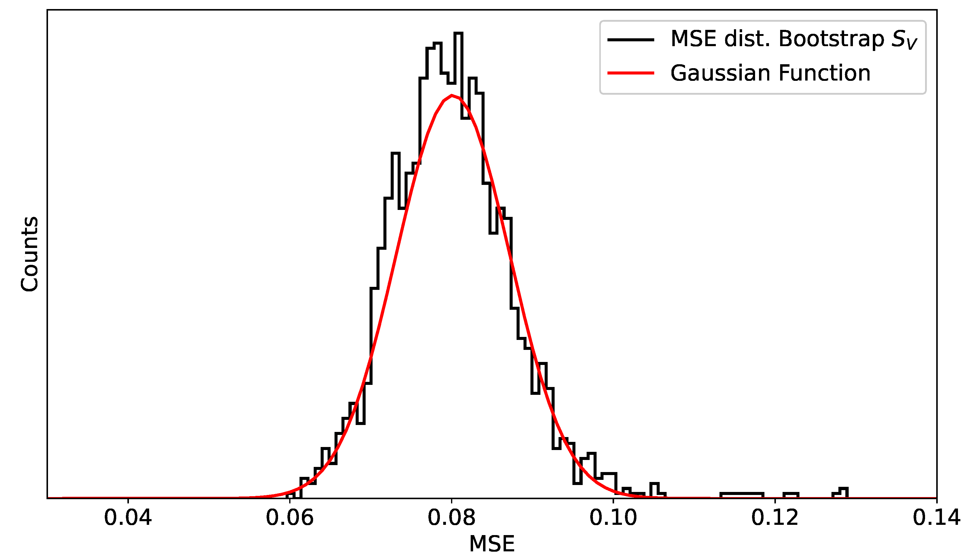
After generating the synthetic data, the dataset was split in 80%, used as a training dataset (), and 20% used for validation (). Then, the bootstrap Algorithm 5 was applied, training the NNM on and generating 1800 bootstrap samples from the datasets. Finally, the MSE metric on the bootstrap samples was evaluated, and its distribution plotted in Figure 2. The black line is the distribution of the MSE on the 1800 bootstrap samples, while the red line is a Gaussian function with the same mean and standard deviations as the evaluated MSE values. Figure 2 shows that, as expected from Corollary 1, the distribution of the MSE values has a Gaussian shape. This justifies, as discussed, the use of the average and standard deviation of the MSE values to completely describe their distribution.
7.2. Comparison of Split/Train and Bootstrap Algorithms
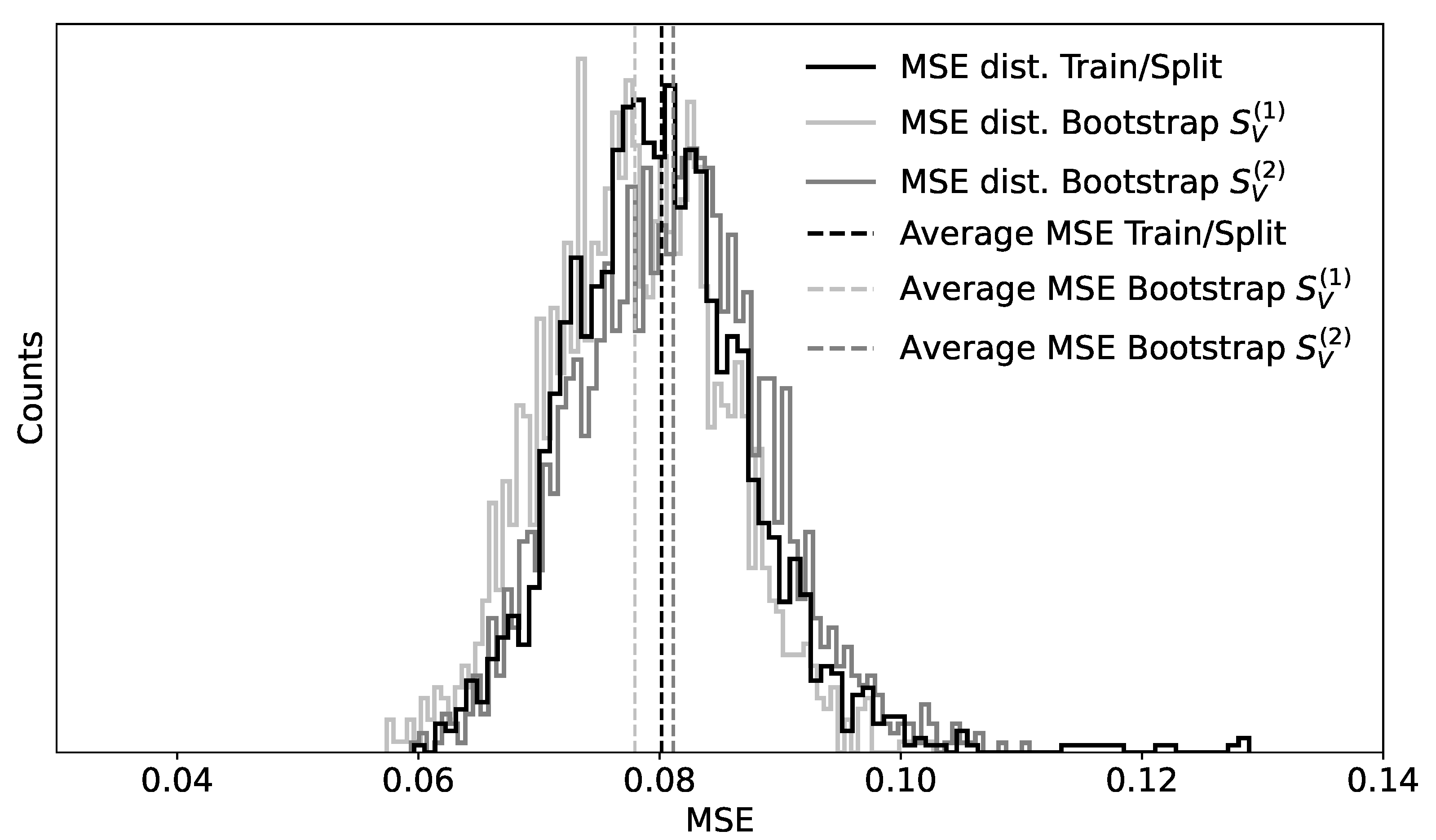
Now let’s compare Algorithms 4 and 5. The results for the MSE metric are summarized in Figure 3. The black line shows the distribution obtained with Algorithm 4. The gray lines are the distributions obtained with Algorithm 5. To illustrate how the distribution depends on the data, was evaluated for two different splits, and . For each of the two cases, a model was trained on the respective training datasets, and , and then Algorithm 5 was applied to and . was used for both Algorithms 4 and 5. The corresponding averages of the metric distributions (vertical dashed lines) are very similar for the shown cases. Note that, depending on the split, the NNM may learn better or worse and, therefore, the average of MSE obtained by using Algorithm 4 may vary, although most of the cases will still be between roughly one of the average obtained by Algorithm 4. The second observation is that, although the average of the MSE may vary a bit, its variance stays quite constant. Finally, the results show that, as expected, the distributions have a Gaussian shape, as expected from Corollary 1. As it was mentioned, Algorithm 5 is computationally more efficient. For example, on a system with an Intel 2.3 Ghz 8-Core i9 CPU, Algorithm 5 took less than a minute, while Algorithm 4 took over an hour.
The comparison between the split/train and bootstrap algorithms is summarized in Table 1, where the average of the MSE, its variance, and the running time are listed. In the Table, the results of k-fold cross-validation and of the mixed approach (a few split/train steps combined with several bootstrap samples) are also reported. Note that for the mixed approach, the reported average of the MSE and are obtained over the several splits.
It is important to note that, in the split/train algorithm, the NNM was trained on 100 different splits, and in the bootstrap algorithm, only on one. To avoid the dependence of the average of the MSE and of its variance on the single split, the mixed approach offers the possibility to check for dependencies from the split still remaining computationally efficient. For comparison, the k-fold CV is computationally efficient, but the distribution of the MSE is composed of very limited (here ) values. Thus, even if the results of Table 1 are numerically similar, the difference is in the computation time and robustness of these values.
8. Application to Real Data
To test the different approaches on real data, the Boston dataset [64] was chosen. This dataset contains house prices collected by the US Census Service in the area of Boston, US. Each observation has 13 features and the target variable is the average price of a house with those features. The interested reader can find the details in [65].
The results are summarized in Table 2. As visible from Table 2, the average of the MSE and its variance obtained with the different algorithms are numerically similar, as obtained on the synthetic dataset. Here, as in the example of Section 7.2, the difference is also in the computation time and robustness of these values.
9. Limitations and Promising Research Developments
It is important to note that the algorithms discussed in this work are presented as practical implementation techniques, but are not based on theoretical mathematical proof, with the exception of Section 3. One of the main obstacles in proving such results is the intractability of neural networks (see, for example, [66]) due to their complexity and non-linearity. Although not yet based on mathematical proofs, those approaches are important tools to be able to estimate the value of a statistical estimator without incurring in problems as described, for example, in the example with the age in the introduction.
The field offers several promising research directions. One interesting question is whether the degradation of the performance of NNMs due to small datasets differs when using the different techniques. This would enable to choose which technique works better with less data. Another promising field is to study different network topologies and the role of the architecture on the resampling results. It is not obvious at all, that different network architectures behave the same when using different resampling results. Finally, it would be important to support the results arising from simulations described in this paper with mathematical proofs. This, in the opinion of the authors, would be one of the most important research directions to pursue in the future.
10. Conclusions
This tutorial showed how the distributions of an average estimator, as the MSE or the accuracy, tends asymptotically to a Gaussian shape. The estimation of the average and variance of such an estimator, the only two parameters needed to describe its distribution, are therefore of great importance when working with NNMs. They allow to assess the performance of an NNM, perceived as its ability to generalise when applied to unseen data.
Classical resampling techniques were explained and discussed, with a focus on their application with NNMs: the hold-out set approach, leave-one-out cross-validation, k-fold cross-validation, jackknife, bootstrap, and split/train. The pseudo-code included is meant to facilitate the implementation. The relevant practical aspects, as with the computation time, were discussed. The application and performance of bootstrap and split/train algorithms were demonstrated with the help of synthetically generated and real data.
The mixed bootstrap algorithm was proposed as a technique to obtain reasonable estimates of the distribution of statistical estimators in a computationally efficient way. The results are comparable with the ones obtained with the much more computationally-intensive algorithms, like the split/train one.
11. Software
The code used in this tutorial for the simulations is available at [67].
Author Contributions
Conceptualization, U.M. and F.V.; methodology, U.M.; software, U.M.; validation, U.M. and F.V.; original draft preparation, U.M.; review and editing, F.V. and U.M. All authors have read and agreed to the published version of the manuscript.
Funding
This research received no external funding.
Data Availability Statement
Not applicable.
Conflicts of Interest
The authors declare no conflict of interest.
Abbreviations
The following abbreviations are used in this manuscript:
| MSE | Mean Square Error |
| NNM | Neural Network Model |
| CLT | Central Limit Theorem |
| iid | independent identically distributed |
| Probability Density Function | |
| LOOCV | Leave-one-out cross-validation |
| CV | cross-validation |
References
- Michelucci, U. Applied Deep Learning—A Case-Based Approach to Understanding Deep Neural Networks; APRESS Media, LLC: New York, NY, USA, 2018. [Google Scholar]
- Izonin, I.; Tkachenko, R.; Verhun, V.; Zub, K. An approach towards missing data management using improved GRNN-SGTM ensemble method. Eng. Sci. Technol. Int. J. 2020. [Google Scholar] [CrossRef]
- Tkachenko, R.; Izonin, I.; Kryvinska, N.; Dronyuk, I.; Zub, K. An Approach towards Increasing Prediction Accuracy for the Recovery of Missing IoT Data based on the GRNN-SGTM Ensemble. Sensors 2020, 20, 2625. [Google Scholar] [CrossRef]
- Izonin, I.; Tkachenko, R.; Vitynskyi, P.; Zub, K.; Tkachenko, P.; Dronyuk, I. Stacking-based GRNN-SGTM Ensemble Model for Prediction Tasks. In Proceedings of the 2020 International Conference on Decision Aid Sciences and Application (DASA), Sakheer, Bahrain, 8–9 November 2020; pp. 326–330. [Google Scholar]
- Alonso-Atienza, F.; Rojo-Álvarez, J.L.; Rosado-Muñoz, A.; Vinagre, J.J.; García-Alberola, A.; Camps-Valls, G. Feature selection using support vector machines and bootstrap methods for ventricular fibrillation detection. Expert Syst. Appl. 2012, 39, 1956–1967. [Google Scholar] [CrossRef]
- Dietterich, T.G. Ensemble Methods in Machine Learning. In Multiple Classifier Systems; Springer: Berlin/Heidelberg, Germany, 2000; pp. 1–15. [Google Scholar]
- Perrone, M.P.; Cooper, L.N. When Networks Disagree: Ensemble Methods for Hybrid Neural Networks; Technical Report; Brown Univ Providence Ri Inst For Brain And Neural Systems: Providence, RI, USA, 1992. [Google Scholar]
- Tkachenko, R.; Tkachenko, P.; Izonin, I.; Vitynskyi, P.; Kryvinska, N.; Tsymbal, Y. Committee of the combined RBF-SGTM neural-like structures for prediction tasks. In International Conference on Mobile Web and Intelligent Information Systems; Springer: Berlin/Heidelberg, Germany, 2019; pp. 267–277. [Google Scholar]
- Sagi, O.; Rokach, L. Ensemble learning: A survey. Wiley Interdiscip. Rev. Data Min. Knowl. Discov. 2018, 8, e1249. [Google Scholar] [CrossRef]
- Tiwari, M.K.; Chatterjee, C. Uncertainty assessment and ensemble flood forecasting using bootstrap based artificial neural networks (BANNs). J. Hydrol. 2010, 382, 20–33. [Google Scholar] [CrossRef]
- Zio, E. A study of the bootstrap method for estimating the accuracy of artificial neural networks in predicting nuclear transient processes. IEEE Trans. Nucl. Sci. 2006, 53, 1460–1478. [Google Scholar] [CrossRef]
- Zhang, J. Inferential estimation of polymer quality using bootstrap aggregated neural networks. Neural Netw. 1999, 12, 927–938. [Google Scholar] [CrossRef]
- Efron, B.; Tibshirani, R.J. An Introduction to the Bootstrap; CRC Press: Boca Raton, FL, USA, 1994. [Google Scholar]
- Good, P.I. Introduction to Statistics through Resampling Methods and R; John Wiley & Sons: Hoboken, NJ, USA, 2013. [Google Scholar]
- Chihara, L.; Hesterberg, T. Mathematical Statistics with Resampling and R; Wiley Online Library: Hoboken, NJ, USA, 2011. [Google Scholar]
- Williams, J.; MacKinnon, D.P. Resampling and distribution of the product methods for testing indirect effects in complex models. Struct. Equ. Model. A Multidiscip. J. 2008, 15, 23–51. [Google Scholar] [CrossRef] [Green Version]
- Montgomery, D.C.; Runger, G.C. Applied Statistics and Probability for Engineers; Wiley: Hoboken, NJ, USA, 2014. [Google Scholar]
- Johnson, N.; Kotz, S.; Balakrishnan, N. Chi-squared distributions including chi and Rayleigh. In Continuous Univariate Distributions; John Wiley & Sons: Hoboken, NJ, USA, 1994; pp. 415–493. [Google Scholar]
- Efron, B. Bootstrap Methods: Another Look at the Jackknife. Ann. Statist. 1979, 7, 1–26. [Google Scholar] [CrossRef]
- Paass, G. Assessing and improving neural network predictions by the bootstrap algorithm. In Advances in Neural Information Processing Systems; Morgan Kaufmann Publishers Inc.: San Francisco, CA, USA, 1992; pp. 196–203. [Google Scholar]
- González-Manteiga, W.; Prada Sánchez, J.M.; Romo, J. The Bootstrap—A Review; Universidad Carlos III de Madrid: Getafe, Spain, 1992. [Google Scholar]
- Lahiri, S. Bootstrap methods: A review. In Frontiers in Statistics; World Scientific: Singapore, 2006; pp. 231–255. [Google Scholar]
- Swanepoel, J. Invited review paper a review of bootstrap methods. S. Afr. Stat. J. 1990, 24, 1–34. [Google Scholar]
- Hinkley, D.V. Bootstrap methods. J. R. Stat. Soc. Ser. B (Methodol.) 1988, 50, 321–337. [Google Scholar] [CrossRef]
- Efron, B. Second thoughts on the bootstrap. Stat. Sci. 2003, 18, 135–140. [Google Scholar] [CrossRef]
- Chernick, M.R. Bootstrap Methods: A Guide for Practitioners and Researchers; John Wiley & Sons: Hoboken, NJ, USA, 2011; Volume 619. [Google Scholar]
- Lahiri, S. Bootstrap methods: A practitioner’s guide-MR Chernick, Wiley, New York, 1999, pp. xiv+ 264, ISBN 0-471-34912-7. J. Stat. Plan. Inference 2000, 1, 171–172. [Google Scholar] [CrossRef]
- Chernick, M.; Murthy, V.; Nealy, C. Application of bootstrap and other resampling techniques: Evaluation of classifier performance. Pattern Recognit. Lett. 1985, 3, 167–178. [Google Scholar] [CrossRef]
- Efron, B. The Jackknife, the Bootstrap and Other Resampling Plans; SIAM: Philadelphia, PA, USA, 1982. [Google Scholar]
- Zainuddin, N.H.; Lola, M.S.; Djauhari, M.A.; Yusof, F.; Ramlee, M.N.A.; Deraman, A.; Ibrahim, Y.; Abdullah, M.T. Improvement of time forecasting models using a novel hybridization of bootstrap and double bootstrap artificial neural networks. Appl. Soft Comput. 2019, 84, 105676. [Google Scholar] [CrossRef]
- Li, X.; Deng, S.; Wang, S.; Lv, Z.; Wu, L. Review of small data learning methods. In Proceedings of the 2018 IEEE 42nd Annual Computer Software and Applications Conference (COMPSAC), Tokyo, Japan, 23–27 July 2018; Volume 2, pp. 106–109. [Google Scholar]
- Reed, S.; Lee, H.; Anguelov, D.; Szegedy, C.; Erhan, D.; Rabinovich, A. Training deep neural networks on noisy labels with bootstrapping. arXiv 2014, arXiv:1412.6596. [Google Scholar]
- Diciccio, T.J.; Romano, J.P. A review of bootstrap confidence intervals. J. R. Stat. Soc. Ser. B (Methodol.) 1988, 50, 338–354. [Google Scholar] [CrossRef]
- Khosravi, A.; Nahavandi, S.; Srinivasan, D.; Khosravi, R. Constructing optimal prediction intervals by using neural networks and bootstrap method. IEEE Trans. Neural Netw. Learn. Syst. 2014, 26, 1810–1815. [Google Scholar] [CrossRef] [PubMed]
- Gonçalves, S.; Politis, D. Discussion: Bootstrap methods for dependent data: A review. J. Korean Stat. Soc. 2011, 40, 383–386. [Google Scholar] [CrossRef]
- Chernick, M.R. The Essentials of Biostatistics for Physicians, Nurses, and Clinicians; Wiley Online Library: Hoboken, NJ, USA, 2011. [Google Scholar]
- Pastore, A. An introduction to bootstrap for nuclear physics. J. Phys. G Nucl. Part Phys. 2019, 46, 052001. [Google Scholar] [CrossRef] [Green Version]
- Sohn, R.; Menke, W. Application of maximum likelihood and bootstrap methods to nonlinear curve-fit problems in geochemistry. Geochem. Geophys. Geosyst. 2002, 3, 1–17. [Google Scholar] [CrossRef]
- Anirudh, R.; Thiagarajan, J.J. Bootstrapping graph convolutional neural networks for autism spectrum disorder classification. In Proceedings of the ICASSP 2019-2019 IEEE International Conference on Acoustics, Speech and Signal Processing (ICASSP), Brighton, UK, 12–17 May 2019; pp. 3197–3201. [Google Scholar]
- Gligic, L.; Kormilitzin, A.; Goldberg, P.; Nevado-Holgado, A. Named entity recognition in electronic health records using transfer learning bootstrapped neural networks. Neural Netw. 2020, 121, 132–139. [Google Scholar] [CrossRef]
- Ruf, J.; Wang, W. Neural networks for option pricing and hedging: A literature review. J. Comput. Financ. 2019, 24, 1–46. [Google Scholar] [CrossRef] [Green Version]
- Efron, B. Better bootstrap confidence intervals. J. Am. Stat. Assoc. 1987, 82, 171–185. [Google Scholar] [CrossRef]
- Gareth, J.; Daniela, W.; Trevor, H.; Robert, T. An Introduction to Statistical Learning: With Applications in R; Spinger: Berlin/Heidelberg, Germany, 2013. [Google Scholar]
- Quenouille, M.H. Approximate tests of correlation in time-series. J. R. Stat. Soc. Ser. B (Methodol.) 1949, 11, 68–84. [Google Scholar]
- Cameron, A.C.; Trivedi, P.K. Microeconometrics: Methods and Applications; Cambridge University Press: Cambridge, UK, 2005. [Google Scholar]
- Miller, R.G. The jackknife—A review. Biometrika 1974, 61, 1–15. [Google Scholar]
- Efron, B. Nonparametric estimates of standard error: The jackknife, the bootstrap and other methods. Biometrika 1981, 68, 589–599. [Google Scholar] [CrossRef]
- Wu, C.F.J. Jackknife, bootstrap and other resampling methods in regression analysis. Ann. Stat. 1986, 14, 1261–1295. [Google Scholar] [CrossRef]
- Efron, B.; Stein, C. The jackknife estimate of variance. Ann. Stat. 1981, 9, 586–596. [Google Scholar] [CrossRef]
- Shao, J.; Wu, C.J. A general theory for jackknife variance estimation. Ann. Stat. 1989, 17, 1176–1197. [Google Scholar] [CrossRef]
- Bickel, P.J.; Boley, N.; Brown, J.B.; Huang, H.; Zhang, N.R. Subsampling methods for genomic inference. Ann. Appl. Stat. 2010, 4, 1660–1697. [Google Scholar] [CrossRef]
- Robinson, D.G.; Storey, J.D. subSeq: Determining appropriate sequencing depth through efficient read subsampling. Bioinformatics 2014, 30, 3424–3426. [Google Scholar] [CrossRef] [PubMed] [Green Version]
- Quiroz, M.; Villani, M.; Kohn, R.; Tran, M.N.; Dang, K.D. Subsampling MCMC—An introduction for the survey statistician. Sankhya A 2018, 80, 33–69. [Google Scholar] [CrossRef] [Green Version]
- Elliott, M.R.; Little, R.J.; Lewitzky, S. Subsampling callbacks to improve survey efficiency. J. Am. Stat. Assoc. 2000, 95, 730–738. [Google Scholar] [CrossRef]
- Paparoditis, E.; Politis, D.N. Resampling and subsampling for financial time series. In Handbook of Financial Time Series; Springer: Berlin/Heidelberg, Germany, 2009; pp. 983–999. [Google Scholar]
- Bertail, P.; Haefke, C.; Politis, D.N.; White, H.L., Jr. A subsampling approach to estimating the distribution of diversing statistics with application to assessing financial market risks. In UPF, Economics and Business Working Paper; Universitat Pompeu Fabra: Barcelona, Spain, 2001. [Google Scholar]
- Chernozhukov, V.; Fernández-Val, I. Subsampling inference on quantile regression processes. Sankhyā Indian J. Stat. 2005, 67, 253–276. [Google Scholar]
- Politis, D.N.; Romano, J.P.; Wolf, M. Subsampling for heteroskedastic time series. J. Econom. 1997, 81, 281–317. [Google Scholar] [CrossRef]
- Politis, D.N.; Romano, J.P.; Wolf, M. Subsampling; Springer Science & Business Media: Berlin/Heidelberg, Germany, 1999. [Google Scholar]
- Delgado, M.A.; Rodrıguez-Poo, J.M.; Wolf, M. Subsampling inference in cube root asymptotics with an application to Manski’s maximum score estimator. Econ. Lett. 2001, 73, 241–250. [Google Scholar] [CrossRef] [Green Version]
- Gonzalo, J.; Wolf, M. Subsampling inference in threshold autoregressive models. J. Econom. 2005, 127, 201–224. [Google Scholar] [CrossRef] [Green Version]
- Politis, D.N.; Romano, J.P. Large sample confidence regions based on subsamples under minimal assumptions. Ann. Stat. 1994, 22, 2031–2050. [Google Scholar] [CrossRef]
- Kingma, D.P.; Ba, J.A. Adam: A method for stochastic optimization. In Proceedings of the 3rd International Conference on Learning Representations, ICLR 2015, San Diego, CA, USA, 7–9 May 2015; pp. 1–15. [Google Scholar]
- Harrison, D., Jr.; Rubinfeld, D.L. Hedonic housing prices and the demand for clean air. J. Environ. Econ. Manag. 1978, 5, 81–102. [Google Scholar] [CrossRef] [Green Version]
- Original paper by Harrison, D.; Rubinfeld, D. The Boston Housing Dataset Website. 1996. Available online: https://www.cs.toronto.edu/~delve/data/boston/bostonDetail.html (accessed on 15 March 2021).
- Jones, L.K. The computational intractability of training sigmoidal neural networks. IEEE Trans. Inf. Theory 1997, 43, 167–173. [Google Scholar] [CrossRef]
- Michelucci, U. Code for Estimating Neural Network’s Performance with Bootstrap: A Tutorial. 2021. Available online: https://github.com/toelt-llc/NN-Performance-Bootstrap-Tutorial (accessed on 20 March 2021).
Figure 1.
A numerical demonstration of the CLT. Panel (a) shows the asymmetric chi-squared distribution of random values for [18], normalized to have the average equal to zero; in panels (b–d), the distribution of the average of the random values is shown for sample size , , and , respectively.
Figure 1.
A numerical demonstration of the CLT. Panel (a) shows the asymmetric chi-squared distribution of random values for [18], normalized to have the average equal to zero; in panels (b–d), the distribution of the average of the random values is shown for sample size , , and , respectively.

Figure 2.
Distribution of the MSE values obtained by evaluating a trained NNM on 1800 bootstrap samples generated from . The NNM used consists of a small neural network with two layers, each having four neurons with the sigmoid activation functions, trained for 250 epochs, with a mini-batch size of 16 with the Adam optimizer.

Figure 3.
Distribution of the MSE values obtained by using Algorithms 4 (black line) and 5 (gray lines). The gray lines were obtained by generating 1800 bootstrap samples from two different validation datasets and , as described in the text. The vertical dashed lines indicate the average of the respective distributions.


Table 1.
Comparison of the average of the MSE and its variance obtained with selected algorithms applied to the synthetic dataset. The running times were obtained on a 23 GHz 8-Core Intel i9 with 32 Gb 2667 MHz DDR4 Memory.
Table 1.
Comparison of the average of the MSE and its variance obtained with selected algorithms applied to the synthetic dataset. The running times were obtained on a 23 GHz 8-Core Intel i9 with 32 Gb 2667 MHz DDR4 Memory.
| Algorithm | <MSE> | Running Time | |
|---|---|---|---|
| Split/Train (100 splits) | 0.098 | 0.01 | 5.8 min |
| Simple Bootrap (100 bootstrap samples) | 0.097 | 0.009 | 5.7 s |
| k-fold cross-validation ( | 0.106 | 0.008 | 0 18 s |
| Mixed approach (10 splits/100 bootstrap samples) | 0.105 | 0.01 | 59 s |
Table 2.
Comparison of the average of the MSE and its variance obtained with selected algorithms applied to the Boston Dataset. The running times were obtained on a 23 GHz 8-Core Intel i9 with 32 Gb 2667 MHz DDR4 Memory. <MSE> and are expressed in the table in 1000 USD.
Table 2.
Comparison of the average of the MSE and its variance obtained with selected algorithms applied to the Boston Dataset. The running times were obtained on a 23 GHz 8-Core Intel i9 with 32 Gb 2667 MHz DDR4 Memory. <MSE> and are expressed in the table in 1000 USD.
| Algorithm | <MSE> | Running Time | |
|---|---|---|---|
| Split/Train (100 splits) | 75.1 | 18.4 | 5.6 min |
| Simple Bootrap (100 bootstrap samples) | 74.7 | 17.8 | 6.2 s |
| k-fold cross-validation ( | 77.2 | 17.2 | 16.7 s |
| Mixed Bootrap (10 splits/100 bootstrap samples) | 75.0 | 15.2 | 63 s |
Publisher’s Note: MDPI stays neutral with regard to jurisdictional claims in published maps and institutional affiliations. |
© 2021 by the authors. Licensee MDPI, Basel, Switzerland. This article is an open access article distributed under the terms and conditions of the Creative Commons Attribution (CC BY) license (http://creativecommons.org/licenses/by/4.0/).
Share and Cite
MDPI and ACS Style
Michelucci, U.; Venturini, F. Estimating Neural Network’s Performance with Bootstrap: A Tutorial. Mach. Learn. Knowl. Extr. 2021, 3, 357-373. https://0-doi-org.brum.beds.ac.uk/10.3390/make3020018
AMA Style
Michelucci U, Venturini F. Estimating Neural Network’s Performance with Bootstrap: A Tutorial. Machine Learning and Knowledge Extraction. 2021; 3(2):357-373. https://0-doi-org.brum.beds.ac.uk/10.3390/make3020018
Chicago/Turabian StyleMichelucci, Umberto, and Francesca Venturini. 2021. "Estimating Neural Network’s Performance with Bootstrap: A Tutorial" Machine Learning and Knowledge Extraction 3, no. 2: 357-373. https://0-doi-org.brum.beds.ac.uk/10.3390/make3020018