A Model of Optimal Interval for Anti-Mosquito Campaign Based on Stochastic Process

Abstract

Mosquito control is very important, in particular, for tropical countries. The purpose of mosquito control is to decrease the number of mosquitos such that the mosquitos transmitted diseases can be reduced. However, mosquito control can be costly, thus there is a trade-off between the cost for mosquito control and the cost for mosquitos transmitted diseases. A model is proposed based on renewal theory in this paper to describe the process of mosquitos’ growth, with consideration of the mosquitos transmitted diseases growth process and the corresponding diseases treatment cost. Through this model, the total mosquitos control cost of different strategies can be estimated. The optimal mosquito control strategy that minimizes the expected total cost is studied. A numerical example and corresponding sensitivity analyses are proposed to illustrate the applications.

1. Introduction

Life and health are the primary human rights and fundamental rights [1,2]. Infectious diseases have a tremendous influence on human life and sometimes they may cause epidemic outbreaks which lead to a great threat on almost all aspects of human society [3,4,5,6,7]. Mosquitos can act as vectors of bacteria, viruses and parasites for many infectious diseases, such as malaria, dengue, West Nile virus, chikungunya, yellow fever, as well as newly detected Keystone virus and Rift Valley fever, which are known as mosquito-borne diseases (MBD) [8,9,10]. Herein, mosquito control is an important issue to governments and health organizations globally. In particular, in tropical countries such as Singapore, the government puts great emphasis on anti-mosquito Campaign [11]. A household may get fined if the government officials find that there is any mosquito or mosquito egg in the house.

With the development of the economy and the progress of biotechnology, governments generally own the ability to launch anti-mosquito campaigns (AMC) which can significantly eradicate mosquitos [12,13,14]. Typical measures include spraying intensive pesticides into the air and getting rid of accumulated water wherein the mosquitos may lay eggs.

Then, this raises an interesting issue, that is, how to develop a strategy of mosquito control. If the interval of AMCs is too long, many people will be infected with MBDs, which can cause a lot of medical expenditure. Frequently launching AMCs may help to limit the mosquito population, but AMCs will cost a large amount of money. Therefore, the need arises to balance the trade-off between the cost of AMCs and the cost of treatment.

Herein, using the stochastic process which is widely used in the field of reliability [15,16,17,18,19,20], a model is proposed to optimize the strategy of mosquito control in this paper. By adjusting the interval of launching AMCs, the aim of our model is to minimize the total cost of the strategy which consists of the cost of launching AMCs and the cost of treatment for the people infected with MBDs.

The remaining of this paper is arranged as follows. Section 2 presents the general model for solving the optimal strategy of mosquito control. Section 3 presents numerical examples to illustrate the optimal interval of launching AMCs. Section 4 provides sensitivity analyses to show how the results are influenced by the variations of the parameters in the proposed model. Section 5 concludes this study.

2. The Cost Model of Mosquito Control Strategy

This paper considers a mosquito control strategy to launch AMCs with a pre-specified interval. The mosquito population will increase with time. Since mosquitos may bring some MBDs to people, the number of patients with diseases spread by mosquitos increases with the size of the mosquito population. Both the cost for AMCs and the cost for the treatments of these patients contribute to the total cost of the mosquito control strategy. The aim of the model is to optimize the interval of AMCs by minimizing the total cost of the mosquito control strategy.

2.1. Mosquito Population Increase

The Verhulst deterministic (VD) model is widely applied to population growth analyses in various biostatical applications. Nevertheless, the traditional VD model does not consider other stochastic factors except the population. For example, people may kill mosquitos themselves in their houses, which leads to a decrease in the mosquito population; if the household waste is not cleaned in time, the mosquito population will increase. Besides human behavior, the speed of mosquitos’ growth is influenced by the weather. Typically, hot weather facilitates the breeding of mosquitos.

In order to take stochastic factors into account, as well as retain the nice properties of the VD model, this paper constructs a stochastic version of the VD model for density-dependent growth of a single population to simulate the growth of mosquito population. Let the mosquito population at time t be represented by $M(t)$. The increasing process of the mosquito population $\left\{M(t):t\in R_{+}\right\}$ is expressed by

$$M(t)=\frac{M_m}{\left[1+(\frac{M_m}{M_0}-1)e^{W(t)}\right]}$$

(1)

where $M_0$ indicates the initial population, $M_m$ indicates the upper limiting population and r indicates the relative growth rate. $W(t)$ is a Wiener-process-based degradation model that can be expressed as

$$W(t)=-rt+\alpha B(0,t), B(0,t) \mathrm{is} \mathrm{standard} \mathrm{Brownian} \mathrm{motion}$$

(2)

where $r>0$ is the drift coefficient, $\alpha >0$ is the diffusion coefficient, and $B(0,t)$ is the standard Brownian motion (BM) representing the stochastic dynamics of the degradation process. Modeling a stochastic degradation process as a Wiener process implies that the mean degradation path is a linear function of time, i.e., $\mathrm{E}\left[W(t)\right]=-rt$. Therefore, the drift parameter $r$ is closely related to the progression of the degradation. In addition, we have the variance of the degradation process $\mathrm{Var}\left[W(t)\right]={\alpha }^{2}t$, which represents the uncertainty of the degradation at time t.

It should be noted that $M_0$ and $M_m$ are input parameters in this model, so they should be known in advance. In practice, they can be estimated in many ways. For example, the sizes of initial population and upper limiting population can be given by experts in biology. Moreover, they can be estimated by field survey using statistics. For instance, researchers can divide the area of a city into many small pieces and then randomly select some pieces to investigate the population of mosquitos on these pieces of land. Finally, the total population can be estimated by the average of the population size from the surveyed areas. Besides, there are some other methods to estimate $M_0$ and $M_m$, since this not the main concern of this study, they are just used as input parameters in this model.

In physical practice, a Wiener process is used to model the movement of small particles with tiny fluctuations in fluids and air. A characteristic feature of this process in the context of reliability is that the plant’s degradation can increase or decrease gradually and accumulatively over time [21]. The small increase or decrease in mosquito population over a small time interval behaves similarly to the random walk of small particles in fluids and air. Therefore, this stochastic process here aims at characterizing the stochastic path of mosquito population where successive fluctuations in population increase can be observed.

According to Equations (1) and (2). It can be inferred that $M(t)$ satisfies following two properties:

(1)

$M(0)=M_0$

Proof:

$$\begin{array}{cc}\hfill M(t=0)& =\frac{M_m}{\left[1+(\frac{M_m}{M_0}-1)e^0\right]}\hfill \\ & =\frac{M_m}{\left[1+(\frac{M_m}{M_0}-1)\right]}\hfill \\ & =M_m\times \frac{M_0}{M_m}\hfill \\ & =M_0\hfill \end{array}$$

(2)

${\lim }_{t\to +\infty }M(t)=M_m$

Proof:

$$\begin{array}{lll}M(t|t\to +\infty )& =& {\lim }_{t\to +\infty }\frac{M_m}{\left[1+(\frac{M_m}{M_0}-1)e^{-r\times t+\alpha B(0,t)}\right]}\\ & =& \frac{M_m}{\left[1+(\frac{M_m}{M_0}-1){\lim }_{t\to +\infty }{e}^{-r\times t+\alpha B(0,t)}\right]}\\ & =& \frac{M_m}{\left[1+(\frac{M_m}{M_0}-1)\times 0\right]}\\ & =& M_m\end{array}$$

From the above two properties, it can be seen that the mosquito population increases from $M_0$ in the beginning and will finally reach its maximum when t is large enough.

In addition, this paper assumes that the AMC is perfect, which means that the AMC can totally eliminate the impact of mosquitos, reducing the mosquito population to $M_0$. In other words, the increasing trend of infection will be terminated and restarted after each AMC.

2.2. MBD Transmission

As a beginning, this paper simplifies the problem by assuming that mosquitos only cause one type of MBD. In practice, though mosquitos can cause different types of MBD, there is usually one predominant type to which one should pay more attention. In addition, this paper assumes that this disease can only be transmitted by mosquitos to uninfected people rather than by infected people to uninfected people. Herein, for a specific region, the infection rate is closely related to the size of the mosquito population.

The Poisson distribution is a discrete probability distribution which is widely used to model the number of event occurrences in an interval of time or space. Here we use it to model the number of transmitted diseases by mosquitos. This study assumes that the number of new infections during the period between two consecutive AMCs is subject to non-homogeneous Poisson distribution with intensity $\lambda (t)$. Generally, the infection rate is increasing with the size of the mosquito population after each AMC. Herein, we assume

$$\lambda (t)=\beta M(t)$$

(3)

where $\beta >0$ is the transmission parameter.

Then, the number of infected people from the time point of AMC to t time units forward can be calculated as

$$\begin{array}{lll}{N}_P(t)& =& {\displaystyle {\int }_0^t\lambda (x)}dx\\ & =& {\displaystyle {\int }_0^t\beta M(x)}dx\\ & =& {\displaystyle {\int }_0^t\frac{\beta M_m}{\left[1+(\frac{M_m}{M_0}-1)e^{-rx+\alpha B(0,x)}\right]}}dx.\end{array}$$

(4)

If we denote the expected number of infected people during [0, t] as $\mathrm{E}\left[N_P(t)\right]$, then the probability that x people are infected during a period of time t can be expressed according to Poisson distribution as

$$P(N_P=x)=\frac{\mathrm{E}{\left[N_P(t)\right]}^x}{x!}{e}^{-\mathrm{E}\left[N_P(t)\right]}$$

(5)

where $x=0,1,2,\dots$.

2.3. Cost Calculation

The cost considered in this study includes the cost of launching AMCs and the medical expenditure because of the people infected with MBD.

For a mosquito control strategy, if the interval of AMCs is $A$ and the time span of the strategy is [0, T], then the total times of AMCs is

$$K=\lfloor \frac{T}{A}\rfloor$$

(6)

where $\lfloor •\rfloor$ is the integer part of $•$. Thus, we know that the time points that launch anti-mosquito campaigns are A, 2A, …, KA. The process is shown as Figure 1.

The total cost of the mosquito control strategy is divided into two parts: the implementation cost of AMCs $C_A$ and the treatment cost $C_D$ of the infected people. We can analyze the total cost mosquito control strategy during the period of [0, T] via Figure 1.

The implementation cost of AMCs includes fixed part and the part influenced by the mosquito population. According to Equations (1) and (2), it can be expressed as

$$\begin{array}{lll}{C}_A& =& K\left[C_{A1}+C_{A2}\mathrm{E}(M(A))\right]\\ & =& \lfloor T/A\rfloor C_{A1}+\lfloor T/A\rfloor C_{A2}E\left[\frac{M_m}{1+(\frac{M_m}{M_0}-1)e^{-rA+\alpha B(0,A)}}\right]\end{array}$$

(7)

where $C_{A1}$ is the fixed coefficient and $C_{A2}$ is the population coefficient. As shown in Equation (7), the first item at the right of the equal sign is only related to the times of AMC, that is the fixed cost; the other item is related to the size of mosquito population.

In Equation (7), $C_A$ is divided into fixed part and varied part. This is a balance between the complexity of the model and the meaning of practice. Generally, if we want to control harmful insects, we will take the same measures in all the possible areas no matter how large the population size of the harmful insects. We do it in this way because it is difficult to estimate the distribution or the density of them in a city or an area. Besides, compared with labor cost, the material cost is usually very less, but the former is comparatively consistent for a different population size of mosquitos in a city or an area. For example, once COVID-19 outbreaks in a city, the government usually carries out the sterilization to the whole city no matter how many people are infected. Thus, we assume that the cost of launching AMC includes a fixed part and a varied part according to the mosquito population size.

The treatment cost of the infected people is estimated based on the number of infected people, which can be formulated as

$$\begin{array}{lll}{C}_D& =& C_P\left\{K\mathrm{E}\left[N_P(A)\right]+\mathrm{E}\left[N_P(T-KA)\right]\right\}\\ & =& C_P\left\{\lfloor T/A\rfloor \mathrm{E}\left[N_P(A)\right]+\mathrm{E}\left[N_P(T-\lfloor T/A\rfloor A)\right]\right\}\\ & =& C_P\lfloor T/A\rfloor {\displaystyle {\int }_0^A\mathrm{E}\left\{\beta M_m/\left[1+(\frac{M_m}{M_0}-1)e^{-rx+\alpha B(0,x)}\right]\right\}}dx\\ & & +C_P{\displaystyle {\int }_0^{T-\lfloor T/A\rfloor A}\mathrm{E}\left\{\beta M_m/\left[1+(\frac{M_m}{M_0}-1)e^{-rx+\alpha B(0,x)}\right]\right\}}dx,\end{array}$$

(8)

where $C_P$ is the treatment cost coefficient indicating the treatment cost for a single person.

Finally, we have the total cost of the mosquito control strategy as

$$C=C_A+C_D$$

(9)

It is noted that since $C_A$ depends on the population size of mosquitos and $C_D$ depends on the number of infected people, $C$ is also varied with the two values.

The expected total cost E(C) can be obtained by averaging the total cost obtained for many simulation runs. By minimizing the expected total cost [22,23], we can obtain the optimal strategy of mosquito control.

3. Numerical Example

Here we consider a strategy of mosquito control during 100 units of time. According to Equations (1) and (2), Figure 2 shows the mosquito population $M(t)$ as a function of t for the case where $M_m={10}^6$, $M_0={10}^4$, $\alpha =1$ and $r=0.5$. It can be seen that the mosquito population generally increases with time from 10,000 though there are significant fluctuations. In particular, the mosquito population explodes during the time between 3 and 5.

For the MBD infection, we present the number of infected people $N_p(t)$ as a function of time t for $\beta =0.01$ in Figure 3. The curve shows a trend of sustained growth. It increases extremely slow because of the small mosquito population. Then, due to the sudden explosion of the mosquito population, the number of infected people rapidly increase.

Assuming $C_{A1}=5000$, $C_{A2}=0.04$ and $C_P=7$, for each simulation run, we can obtain $M(t)$ and $N_p(t)$. Then the total cost of mosquito control strategy can be calculated according to Equation (9). The expected total cost is obtained by averaging the total cost obtained for 100 simulation runs. Figure 4 shows the expected total cost E(C) as a function of A for this example.

It can be seen from Figure 4 that when $A=3$, the expected total cost reaches its minimum value, which is about 311608. In other words, the optimal strategy of mosquito control is launching AMCs with an interval of 3 units of time.

4. Sensitivity Analyses

To investigate how the expected total cost and optimal strategy are influenced by the variation of the parameters, the sensitivity analyses are presented in this section. To maintain the consistency of the numerical example, we only vary the parameters concerned in sensitivity analyses one at a time and set other parameters the same as in Section 3.

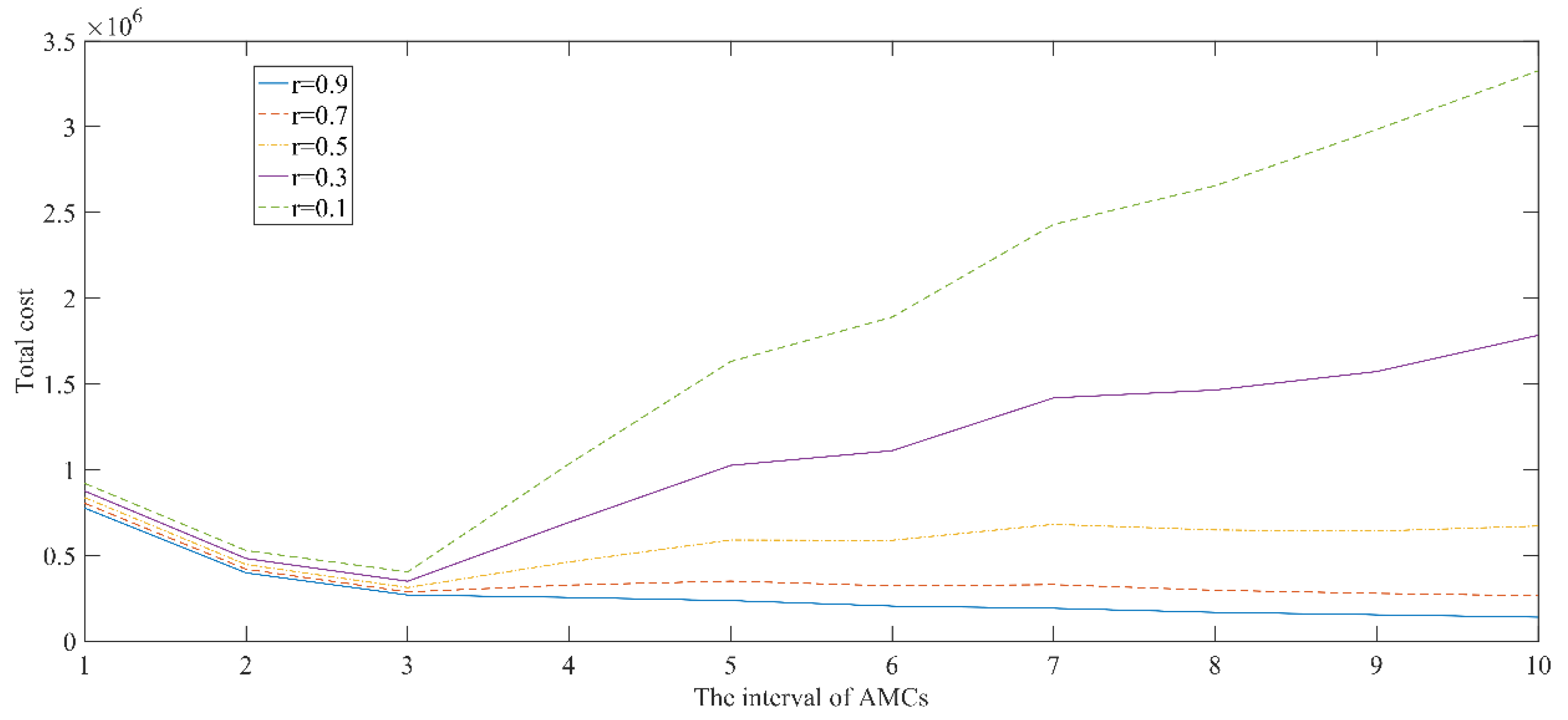
4.1. Drift Parameter r

The first sensitivity analysis is performed for the drift parameter r in Equation (2). We set $M_m={10}^6$, $M_0={10}^4$, $\alpha =1$, $\beta =0.01$, $C_{A1}=5000$, $C_{A2}=0.04$ and $C_P=7$. Then we can obtain the expected total cost based on the proposed model, as shown in Figure 5. It can be seen that all curves decrease with the prolonging of the interval of AMCs when A is no more than 3. However, these curves show different trends while $A>3$. Specifically, when r is small (r = 0.1 or 0.3), the expected total cost maintains the decreasing trend while $A>3$. However, when r is comparatively larger (r = 0.5, 0.7 or 0.9), the expected total cost turns to increase. In fact, when the r is big, the increasing speed of mosquito population may be very quick, thus too long an interval for mosquito control may lead to a great treatment cost. When r is small, the mosquito population is relatively under control even without human intervention, thus it is needed to control the mosquito too often.

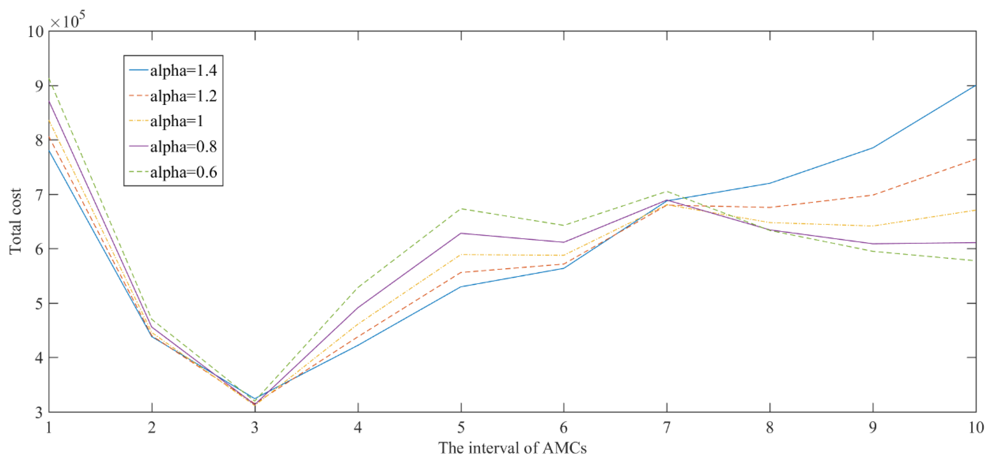
4.2. Diffusion Parameter $\alpha$

The second sensitivity analysis is performed for the diffusion parameter $\alpha$ in Equation (2). We set $M_m={10}^6$, $M_0={10}^4$, $r=0.5$, $\beta =0.01$, $C_{A1}=5000$, $C_{A2}=0.04$ and $C_P=7$. Then we can obtain the expected total cost based on the proposed model, as shown in Figure 6. It can be seen that all curves decrease with the prolonging of the interval of AMCs before $A=3$ and then turn to increase until A reaches 7. In fact, when A is not very big, the increasing speed of the mosquito population is still dominated by r instead of $\alpha$. As analyzed for the case where r = 0.5 for Figure 5, the expected cost when A is smaller than 7 in Figure 6 also presents the same trend as in Figure 5, i.e., it first decreases with A and then increases with A. However, when A is bigger than 7, the $\alpha$ starts to play a more important role. For a big $\alpha$, too long a control interval may lead to a very big mosquito population in some cases, thus leading to the increase of expected total cost for A > 7. When $\alpha$ is not big, the mosquito population growth is slow even for a big A, thus the expected total cost decreases with A due to reduced control cost.

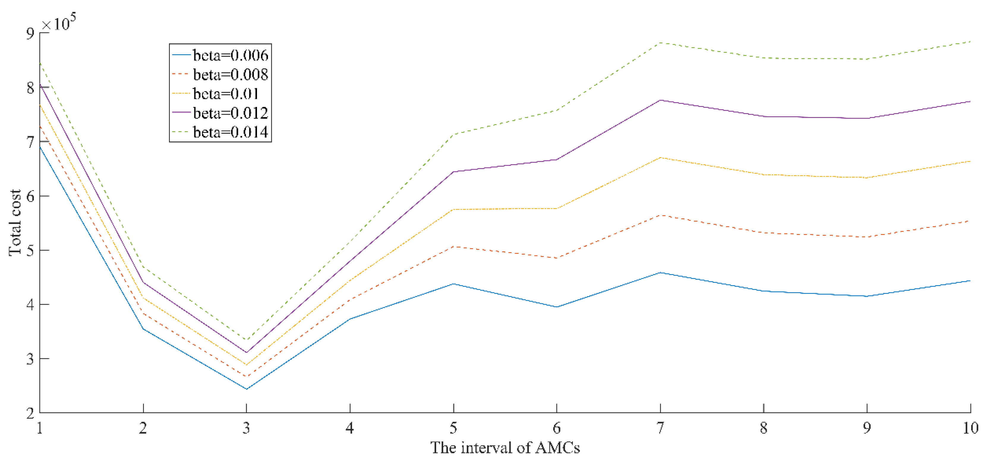
4.3. Transmission Parameter $\beta$

The third sensitivity analysis is performed for the transmission parameter $\beta$ in Equation (3). We set $M_m={10}^6$, $M_0={10}^4$, $r=0.5$, $\alpha =1$, $C_{A1}=5000$, $C_{A2}=0.04$ and $C_P=7$. Then we can obtain the expected total cost based on the proposed model, as shown in Figure 7. It can be seen that the trends of all curves are generally the same and the total costs with bigger $\beta$ are higher. Besides, it should be noted that a bigger $\beta$ accelerates the increase of total cost with interval A when $A>3$. In other words, total cost and its increasing rate are positively related to the transmission rate of MBD. It is consistent with intuition. Actually, no matter the growing pattern of mosquito growth, a big transmission rate always leads to a greater cost.

4.4. Initial Population $M_0$ and Upper Limiting Population $M_m$

The fourth sensitivity analysis is performed for the initial population $M_0$ and the upper limiting population $M_m$ in Equation (1). We set $r=0.5$, $\alpha =1$, $\beta =0.01$, $C_{A1}=5000$, $C_{A2}=0.04$ and $C_P=7$. Then we can obtain the expected total cost based on the proposed model, as shown in Figure 8. The result in this sensitivity analysis is similar to the result of sensitivity analysis for the transmission parameter $\beta$. The increases of both $M_0$ and $M_m$ can lead to a growth of the total cost and its increasing rate with interval A. Herein, total cost and its increasing rate are also positively related with the initial population and the upper limiting population.

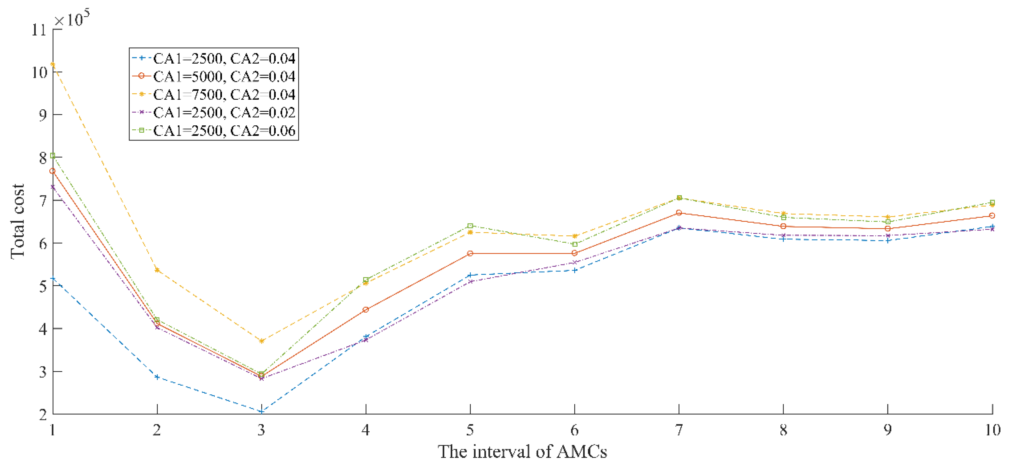
4.5. Fixed Coefficient $C_{A1}$ and Population Coefficient $C_{A2}$

The fifth sensitivity analysis is performed for is the fixed coefficient $C_{A1}$ and the population coefficient $C_{A2}$ in Equation (7). We set $M_m={10}^6$, $M_0={10}^4$, $r=0.5$, $\alpha =1$,$\beta =0.01$ and $C_p=1$ Then we can obtain the total cost based on the proposed model, as shown in Figure 9. The variation of $C_{A1}$ and $C_{A2}$ generally cannot change the trend of the total cost with interval A, that is, these curves first decrease to the minimum at $A=3$ and then increase until $A=7$ as well as finally become stable when $A>7$. It should be noted that the gaps between different curves decreases with the interval A, which is also divided into three stages by A when $A=3$ and $A=7$. This finding illustrates that the cost of AMCs is more important to the total cost when the interval of AMCs is shorter. In addition, the increasing rate is significantly influenced by the population coefficient $C_{A2}$ when $A>3$.

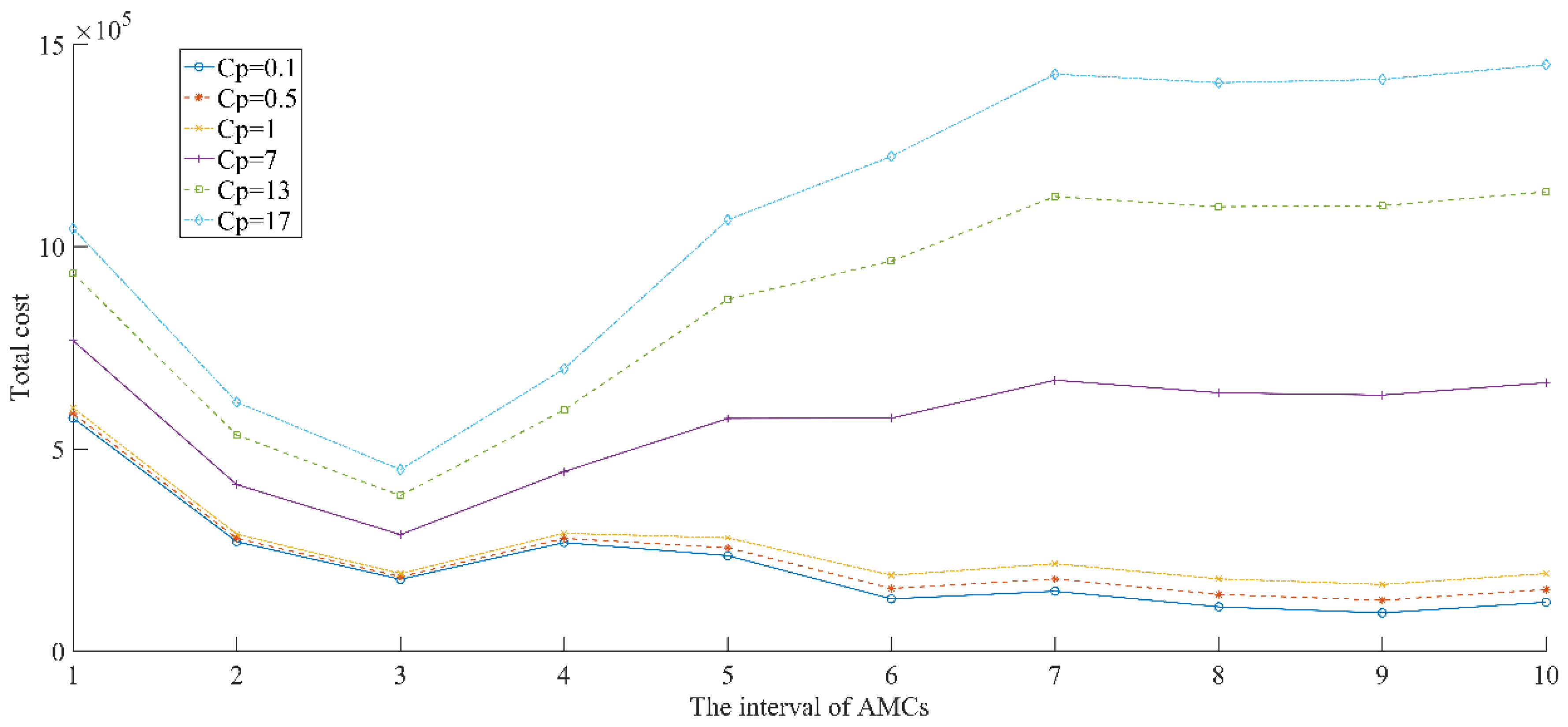
4.6. Treatment Cost Coefficient $C_P$

The last sensitivity analysis is performed for the treatment cost coefficient $C_P$ in Equation (8). We set $M_m={10}^6$, $M_0={10}^4$, $r=0.5$, $\alpha =1$, $\beta =0.01$, $C_{A1}=5000$ and $C_{A2}=0.04$. Then we can obtain the total cost based on the proposed model, as shown in Figure 10. The variation of $C_P$ generally cannot change the trend of these curves with interval A when $A<3$. However, it should be noted that the curves with bigger $C_P$ are higher than the curves with smaller $C_P$. In addition, the increasing trend of these curves is also largely altered for different values of $C_P$. Bigger can accelerate the increasing rate. In the cases where $C_P$ is very small ($C_P=0.1, 0.5 \mathrm{or} 1$), the total cost reaches its minimum value even when $A>3$, which means the optimal strategy is changed. The result in this sensitivity analysis proves that the treatment cost can largely influence the mosquito control strategy both in total cost and the optimal interval of AMCs.

5. Conclusions

This paper mainly discusses the optimal strategy of mosquito control based on the renewal theory. Firstly, based on the applications of existing technology and the practice situation of mosquito control, we propose an interesting research topic, that is, by minimizing the cost to obtain the optimal strategy of mosquito control. Then, we analyze the mosquito population increase and the disease transmission. Next, considering the mosquito population and the people infected by mosquitos, we provide a model to calculate the total cost for a mosquito control strategy and the expected total cost is obtained from simulation results. Finally, a numerical example is presented to illustrate the proposed model and the corresponding sensitivity analyses are performed. The results of the numerical example show that the optimal strategy can be found using the proposed model. The results of sensitivity analyses prove that the optimal strategy and its total cost are altered with the variation of parameters in the proposed model.

References

- Czakó, B.; Kovács, L. Nonlinear Model Predictive Control Using Robust Fixed Point Transformation-Based Phenomena for Controlling Tumor Growth. Machines 2018, 6, 49. [Google Scholar] [CrossRef] [Green Version]
- Gao, K.; Shi, X.; Wang, W. The life-course impact of smoking on hypertension, myocardial infarction and respiratory diseases. Sci. Rep. 2017, 7, 4330. [Google Scholar] [CrossRef] [PubMed] [Green Version]
- Alonso-Quesada, S.; De la Sen, M.; Nistal, R. An SIRS Epidemic Model Supervised by a Control System for Vaccination and Treatment Actions Which Involve First-Order Dynamics and Vaccination of Newborns. Mathematics 2022, 10, 36. [Google Scholar] [CrossRef]
- Samanta, G.P.; Sen, P.; Maiti, A. A delayed epidemic model of diseases through droplet infection and direct contact with saturation incidence and pulse vaccination. Syst. Sci. Control Eng. 2016, 4, 320–333. [Google Scholar] [CrossRef] [Green Version]
- Tsuji, B.T.; Pogue, J.M.; Zavascki, A.P.; Paul, M.; Daikos, G.L.; Forrest, A.; Giacobbe, D.R.; Viscoli, C.; Giamarellou, H.; Karaiskos, L.; et al. International consensus guidelines for the optimal use of the polymyxins endorsed by the American College of Clinical Pharmacy (ACCP), European Society of Clinical Microbiology and Infectious Diseases (ESCMID), Infectious Diseases Society of America (IDSA), International Society for Anti-infective Pharmacology (ISAP), Society of Critical Care Medicine (SCCM), and Society of Infectious Diseases Pharmacists (SIDP). Pharmacotherapy 2019, 39, 10–39. [Google Scholar] [PubMed]
- Pereira, M.R.; Mohan, S.; Cohen, D.J.; Husain, S.A.; Dube, G.K.; Ratner, L.E.; Arcasoy, S.; Aversa, M.M.; Benvenuto, L.J.; Dadhania, D.M.; et al. COVID-19 in solid organ transplant recipients: Initial report from the US epicenter. Am. J. Transplant. 2020, 20, 1800–1808. [Google Scholar] [CrossRef]
- Ivanov, D. Predicting the impacts of epidemic outbreaks on global supply chains: A simulation-based analysis on the coronavirus outbreak (COVID-19/SARS-CoV-2) case. Transp. Res. Part E-Logist. Transp. Rev. 2020, 136, 101922. [Google Scholar] [CrossRef]
- Reiter, P. Climate change and mosquito-borne disease. Environ. Health Perspect. 2001, 109, 141–161. [Google Scholar]
- Hay, S.I.; Myers, M.F.; Burke, D.S.; Vaughn, D.W.; Endy, T.; Ananda, N.; Shanks, G.D.; Snow, R.W.; Rogers, D.J. Etiology of interepidemic periods of mosquito-borne disease. Proc. Natl. Acad. Sci. USA 2000, 97, 9335–9339. [Google Scholar] [CrossRef] [Green Version]
- Dye, C. Population dynamics of mosquito-borne disease: Effects of flies which bite some people more frequently than others. Trans. R. Soc. Trop. Med. Hyg. 1986, 80, 69–77. [Google Scholar] [CrossRef]
- Burattini, M.N.; Chen, M.; Chow, A.; Coutinho, F.A.B.; Goh, K.T.; Lopez, L.F.; Ma, S.; Massad, E. Modelling the control strategies against dengue in Singapore. Epidemiol. Infect. 2008, 136, 309–319. [Google Scholar] [CrossRef] [PubMed]
- Lal, A.A.; Patterson, P.S.; Sacci, J.B.; Vaughan, J.A.; Paul, C.; Collins, W.E.; Wirtz, R.A.; Azad, A.F. Anti-mosquito midgut antibodies block development of Plasmodium falciparum and Plasmodium vivax in multiple species of Anopheles mosquitoes and reduce vector fecundity and survivorship. Proc. Natl. Acad. Sci. USA 2001, 98, 5228–5233. [Google Scholar] [CrossRef] [Green Version]
- Curtis, C.F. Malaria control through anti-mosquito measures. J. R. Soc. Med. 1989, 82, 18–21. [Google Scholar] [PubMed]
- Headlee, J.T. Anti-mosquito work in New Jersey. J. Econ. Entomol. 1914, 7, 260–268. [Google Scholar] [CrossRef]
- Gao, K.; Peng, R.; Qu, L.; Wu, S. Jointly optimizing lot sizing and maintenance policy for a production system with two failure modes. Reliab. Eng. Syst. Saf. 2020, 202, 106996. [Google Scholar] [CrossRef]
- Peng, R.; Li, G.; Levitin, G.; Mo, H.D.; Wang, W. Maintenance versus individual and overarching protections for parallel systems. Qual. Technol. Quant. Manag. 2014, 11, 353–362. [Google Scholar] [CrossRef]
- Liu, Y.; Li, Y.; Huang, H.Z.; Zuo, M.J.; Sun, Z. Optimal preventive maintenance policy under fuzzy Bayesian reliability assessment environments. IIE Trans. 2010, 42, 734–745. [Google Scholar] [CrossRef]
- Gao, K.; Yan, X.; Peng, R.; Xing, L. Economic design of a linear consecutively connected system considering cost and signal loss. IEEE Trans. Syst. Man Cybern.-Syst. 2021, 51, 5116–5128. [Google Scholar] [CrossRef]
- Dulf, E.H.; Saila, M.; Muresan, I.C.; Miclea, L.C. An Efficient Design and Implementation of a Quadrotor Unmanned Aerial Vehicle Using Quaternion-Based Estimator. Mathematics 2020, 8, 1829. [Google Scholar] [CrossRef]
- Muresan, C.I.; Birs, I.R.; Dulf, E.H. Event-Based Implementation of Fractional Order IMC Controllers for Simple FOPDT Processes. Mathematics 2020, 8, 1378. [Google Scholar] [CrossRef]
- Si, X.S.; Wang, W.; Hu, C.H.; Chen, M.Y.; Zhou, D.H. A wiener-process-based degradation model with a recursive filter algorithm for remaining useful life estimation. Mech. Syst. Signal Process. 2013, 35, 219–237. [Google Scholar] [CrossRef]
- Yang, L.; Chen, Y.; Qiu, Q.; Wang, J. Risk control of mission-critical systems: Abort decision-makings integrating health and age conditions. IEEE Trans. Ind. Inform. 2022. [Google Scholar] [CrossRef]
- Zhang, Z.; Yang, L. State-based opportunistic maintenance with multifunctional maintenance windows. IEEE Trans. Reliab. 2021, 70, 1481–1494. [Google Scholar] [CrossRef]
Figure 1.
The mosquito control strategy.
Figure 2.
The mosquito population as a function of t for the case where , , and .
Figure 3.
The number of infected people as a function of time t for .
Figure 4.
The expected total cost E(C) as a function of A for , and .
Figure 5.
Expected total cost C vs. A for , ,, , , , , as well as for different values of r.
Figure 6.
Expected total cost C vs. A for , , , , , , , as well as for different values of .
Figure 7.
Expected total cost C vs. A for , , , , , and , as well as for different values of .
Figure 8.
Expected total cost C vs. A for , , , , , , as well as for different values of and .
Figure 9.
Expected total cost C vs. A for, , , , , , as well as for different values of and .
Figure 10.
Expected total cost C vs. A for as well as for different values of Cp.
Publisher’s Note: MDPI stays neutral with regard to jurisdictional claims in published maps and institutional affiliations. |
© 2022 by the authors. Licensee MDPI, Basel, Switzerland. This article is an open access article distributed under the terms and conditions of the Creative Commons Attribution (CC BY) license (https://creativecommons.org/licenses/by/4.0/).
Share and Cite
MDPI and ACS Style
Lei, B.; Gao, K.; Yang, L.; Fang, S. A Model of Optimal Interval for Anti-Mosquito Campaign Based on Stochastic Process. Mathematics 2022, 10, 440. https://0-doi-org.brum.beds.ac.uk/10.3390/math10030440
AMA Style
Lei B, Gao K, Yang L, Fang S. A Model of Optimal Interval for Anti-Mosquito Campaign Based on Stochastic Process. Mathematics. 2022; 10(3):440. https://0-doi-org.brum.beds.ac.uk/10.3390/math10030440
Chicago/Turabian StyleLei, Bingyin, Kaiye Gao, Li Yang, and Shu Fang. 2022. "A Model of Optimal Interval for Anti-Mosquito Campaign Based on Stochastic Process" Mathematics 10, no. 3: 440. https://0-doi-org.brum.beds.ac.uk/10.3390/math10030440
Note that from the first issue of 2016, this journal uses article numbers instead of page numbers. See further details here.