On Estimating the Parameters of the Beta Inverted Exponential Distribution under Type-II Censored Samples


Department of Statistics, College of Science, University of Jeddah, Jeddah 21589, Saudi Arabia
*
Author to whom correspondence should be addressed.
Mathematics 2022, 10(3), 506; https://0-doi-org.brum.beds.ac.uk/10.3390/math10030506
Submission received: 13 November 2021
/
Revised: 1 January 2022
/
Accepted: 27 January 2022
/
Published: 5 February 2022
(This article belongs to the Section Probability and Statistics)
Abstract
:This article aims to consider estimating the unknown parameters, survival, and hazard functions of the beta inverted exponential distribution. Two methods of estimation were used based on type-II censored samples: maximum likelihood and Bayes estimators. The Bayes estimators were derived using an informative gamma prior distribution under three loss functions: squared error, linear exponential, and general entropy. Furthermore, a Monte Carlo simulation study was carried out to compare the performance of different methods. The potentiality of this distribution is illustrated using two real-life datasets from difference fields. Further, a comparison between this model and some other models was conducted via information criteria. Our model performs the best fit for the real data.
Keywords:
Bayes estimators; beta inverted exponential distribution; generalized hypergeometric function; loss functions; maximum likelihood estimators; simulation study; type-II censored samplesMSC:
62F10; 62F15; 62G05; 62N01; 65C051. Introduction
In many life-testing and reliability studies for engineering or medical sciences, the information on failure times for all experimental units may not be obtained ultimately by the experimenter. Due to this, there are many situations in which it is pre-planned to remove units before failure, and these obtained data are called censored data. The most common censoring schemes in life-testing experiments are type-I and type-II censoring schemes. The type-II censoring scheme is used often in toxicology experiments and life-testing applications, where it has proven to save time and money. Many authors have addressed Bayesian and non-Bayesian estimations based on type-II censored samples or different types of samples, including [1], who derived maximum likelihood estimation (MLE) and Bayes estimation under different types of loss functions for exponentiated Weibull distribution based on type-II censored samples. Prakash [2] discussed the properties of the Bayes estimator and the minimax estimator of the parameter of the inverted exponential distribution. The moments of the lower record value and the estimation of the parameter were presented, based on a series of observed record values by the maximum likelihood (ML). Furthermore, Dey and Dey [3] derived the MLE of the generalized inverted exponential distribution parameters in the case of the progressive type-II censoring scheme with binomial removals. Singh and Goel [4] studied a three-parameter beta inverted exponential distribution (BIED). They derived the non-central moments, inverse moments, moment-generating function, inverse-moment-generating function, and mode. Furthermore, they examined the distributional properties of order statistics. Moreover, a statistical inference about the distribution parameters based on a complete sample was investigated. Garg et al. [5] studied the MLE of the parameters and the expected Fisher information under a random censoring model of the generalized inverted exponential distribution. Bakoban and Abu-Zinadah [6] considered the four-parameter beta generalized inverted exponential distribution for complete samples. In their research, the MLE, the Fisher information matrix, and the confidence interval were found. Besides that, the Monte Carlo simulation was discussed to illustrate the theoretical results of the estimation. Finally, applications on real datasets were provided. Aldahlan [7] applied the ML method to estimate the inverse Weibull inverse exponential distribution parameters. One real dataset about time between failures for repairable items was applied. This article focuses on estimation methods based on the type-II censoring scheme. Two estimation methods were used to estimate the unknown parameters for the beta inverted exponential distribution (BIED): MLE and Bayes estimation. The proposed distribution has three parameters (scale parameter and shape parameters and ). The cumulative distribution function (CDF) and the probability density function (PDF) of BIED, respectively, are:
and:
where is the beta function. Equation (1) could also be written as a regularized incomplete beta function:
where is the incomplete beta function, such that:
The inverse of CDF is called the quantile function and is given by:
The survival and hazard function of the BIED, respectively, are given by:
and:
The layout of this article is as follows: In Section 2, the estimation of the unknown parameters for the BIED under type-II censored samples is introduced. A simulation study is discussed in Section 3. In Section 4, an application with real data is provided. Finally, the conclusion is given in Section 5.
2. Method of Estimation
In this section, we derive the ML and Bayesian estimators for the unknown parameters of the BIED based on type-II censored samples.
2.1. Maximum Likelihood Estimation
Assume that are a random sample from the BIED and the order statistics of this sample are . The rth observations were chosen in type-II censored sample . The likelihood function of the type-II censored sample is given by (see [8]):
By substituting Equations (2) and (3) in (8), the likelihood function for the vector is given by:
Then, the log-likelihood function can be expressed as follows:
The partial derivatives of the log-likelihood function with respect to , , and are given as:
where:
According to Abramowitz and Stegun [9], is called the Psi (or digamma) function. Then:
By using and taking , we obtain the partial derivatives of :
Equation (12) can be rewritten as:
where is called the regularized hypergeometric function and is the generalized hypergeometric function, and denotes the ascending factorial (Pochhammer symbol) (see [10]).
Next,
where:
then:
By using , we obtain:
2.2. Bayes Estimation
Bayes estimators for the BIED are obtained based on type-II censored samples in this subsection. Singh and Goel [4] derived the Bayes estimators for the BIED based on complete samples under the SE loss function. They considered the gamma prior distribution for the unknown BIED parameters. The prior distribution is denoted by , which tells us what is known about without observing the data. Bayes theorem is based on the posterior distribution, which is defined as and given by (see [11]):
where is continuous and is the likelihood function. Furthermore, Equation (19) could be written as:
where k is called the normalizing constant, necessary to ensure that the posterior distribution integrates or sums to one.
Here, we derive the Bayes estimates for , and under three types of loss functions: squared error (SE), linear exponential (LINEX), and general entropy (GE). Moreover, four cases are considered first when is unknown, while and are known. A second case is when is unknown, while are known. A third case is when the scale parameter is unknown. Finally, a fourth case is when both and are unknown. Two techniques are used to compute the estimates: the standard Bayes and importance sampling techniques for the first three cases. The last case is computed via the importance sampling technique.
2.2.1. Case 1: Bayes Estimators When Is Unknown
Assume is unknown and has the following prior distribution ; thus, the prior for is given by:
By combining (9) and (21), the posterior distribution of the unknown parameter is given by:
where is the normalizing constant, defined as:
Therefore, the Bayes estimator of , denoted by , is obtained under three types of loss functions and two techniques as follows.
- SE Loss Function
The symmetric loss function SE is defined as:
Then, the Bayes estimator of under the SE loss function, denoted by , and can be found using Equations (24) and (22).
where is defined in Equation (23).
- ii.
- LINEX Loss Function
Varian [12] proposed the LINEX loss function as follows:
The Bayes estimator of under the LINEX loss function, denoted by , can be found by using Equations (26) and (22).
where is defined in (23).
- iii.
- GE Loss Function
According to Calabria and Pulcini [13], the GE loss function of can be defined as:
The Bayes estimator of under the GE loss function, denoted by , can be found by using Equations (22) and (28).
where is defined in (23).
The Bayes estimator of using the importance sampling technique can be derived by rewriting the posterior density function in Equation (22); thus:
The posterior density function of can be considered as:
where:
The Bayes estimators of under the SE, LINEX, and GE loss functions based on the importance sampling technique, denoted by and , respectively, could be found using the following Algorithm 1.
where
| Algorithm 1 Importance sampling technique when is unknown based on type-II censored samples. |
|
The Bayes estimators of are found numerically under these three loss functions by the NIntegrate function via Mathematica 11.
2.2.2. Case 2: Bayes Estimators When Is Unknown
Suppose is unknown and has the following prior distribution , given by:
By combining (9) and (35), the posterior distribution of the unknown parameter is given by:
where is the normalizing constant and can be written as:
Therefore, the Bayes estimator of , denoted by , is obtained under three types of loss function and two techniques as follows.
- SE Loss Function
The Bayes estimator of under the SE loss function, denoted by , can be found by using Equations (24) and (36).
where is defined in Equation (37).
- ii.
- LINEX Loss Function
The Bayes estimator of under the LINEX loss function, denoted by , can be found by using Equations (26) and (36).
where is defined in (37).
- iii.
- GE Loss Function
The Bayes estimator of under the GE loss function, denoted by , can be found by using Equations (28) and (36).
where is defined in (37).
The Bayes estimator of using the importance sampling technique can be derived by rewriting the posterior density function in Equation (36); thus:
The posterior density function of can be considered as:
where:
The Bayes estimators of under the SE, LINEX, and GE loss functions based on the importance sampling technique, denoted by and , respectively, could be found using the following Algorithm 2.
where
| Algorithm 2 Importance sampling technique when is unknown based on type-II censored samples. |
|
The Bayes estimators of under the three loss functions cannot be computed analytically through the two techniques used. They can be found numerically using the NIntegrate function via Mathematica 11.
2.2.3. Case 3: Bayes Estimators When Is Unknown
Suppose that the scale parameter is unknown and has the following prior distribution , given by:
By combining (9) and (46), the posterior distribution of the unknown parameter is given by:
where is the normalizing constant and can be written as:
The Bayes estimator of is indicated by , and this estimator is obtained under three types of loss function and two techniques as follows.
- SE Loss Function
The Bayes estimator of under the SE loss function, denoted by , can be found by using Equations (24) and (47).
where is defined in Equation (48).
- ii.
- LINEX Loss Function
The Bayes estimator of under the LINEX loss function, denoted by , can be found by using Equations (26) and (47).
where is defined in (48).
- iii.
- GE Loss Function
The Bayes estimator of under the GE loss function, denoted by , can be found by using Equations (28) and (47).
where is defined in (48).
The Bayes estimator of using the importance sampling technique can be obtained by rewriting the posterior density function in Equation (47); thus:
The posterior density function of can be considered as:
where:
The Bayes estimators of under the SE, LINEX, and GE loss functions based on the importance sampling technique, denoted by and , respectively, could be found using the following Algorithm 3.
where
| Algorithm 3 Importance sampling technique when is unknown based on type-II censored samples. |
|
The Bayes estimators of under the three loss functions cannot be computed analytically through the two techniques used. It can be found numerically using the NIntegrate function via Mathematica 11.
2.2.4. Case 4: Bayes Estimators When and Are Unknown
Consider that both parameters and are unknown. Suppose and . Therefore, the joint prior distribution is given by:
By combining (9) and (57), the joint posterior distribution of the unknown parameters and is given by:
where is the normalizing constant and can be written as:
The Bayes estimators of and are derived under three types of loss function as follows.
- SE Loss Function
The Bayes estimators of under the SE loss function, denoted by , can be found by using Equations (24) and (58).
where is defined in Equation (59).
Different forms of the Bayes estimator for are obtained from Equation (60):
- ii.
- LINEX Loss Function
The Bayes estimator of under the LINEX loss function, denoted by , can be found by using Equations (26) and (58).
where is defined in (59).
Different forms of the Bayes estimator for are obtained from Equation (63):
- iii.
- GE Loss Function
The Bayes estimator of under the GE loss function, denoted by , can be found by using Equations (28) and (58).
where is defined in (59).
Different forms of the Bayes estimator for are obtained from Equation (66):
The Bayes estimators of and can be obtained using the importance sampling technique by rewriting the joint posterior density function of and in Equation (58) as follows:
The joint posterior density function of and can be considered as:
where:
The Bayes estimators of under the SE, LINEX, and GE loss functions based on the importance sampling technique, denoted by and , respectively, could be found using the following Algorithm 4.
where
| Algorithm 4 Importance sampling technique when and are unknown based on type-II censored samples. |
|
The Bayes estimators of and under the three loss functions can be found numerically using the NIntegrate function via Mathematica 11.
3. Simulation Study
Simulation studies were conducted using Mathematica 11 to clarify the performance of the proposed estimators. Simulation results are given for the ML and Bayesian methods based on type-II censored samples. Furthermore, biases and mean-squared errors (MSE) were considered to illustrate the performance of the different estimators, defined as:
The ML estimates of the parameters , , and could be found using the following Algorithm 5.
| Algorithm 5 ML method of the parameters , , and based on type-II censored samples. |
|
Three different sets of true parameter values were selected to perform the simulation. Furthermore, different sample sizes and 100 and two censoring percentage of and were selected. Table 1 shows the ML estimates for , , , , the bias, and the MSE for the true values and , at . The ML estimates for , , , , the bias, and the MSE for the true values and , at are summarized in Table 2. Moreover, for the true values and , at , the ML estimates for , , , , the bias, and the MSE are listed in Table 3.
It is clear from Table 1, Table 2 and Table 3 that the MSEs of the estimates decrease as the sample size increases. Based on biases, the parameter was underestimated for all sets of true values, except in Table 2, the parameter was overestimated. Likewise, the parameter was overestimated. Besides, we noticed that when the percentage of censoring was , the MSE of the estimates in most cases was better.
Bayes estimates of the parameters , , , and could be found using the following Algorithm 6.
| Algorithm 6 Bayesian method of the parameters , , , and based on type-II censored samples. |
|
The simulation study was carried out with the true value of parameter , , and different sample sizes and 100 for all four cases. Furthermore, we considered three different values of the LINEX shape parameter and three values of the GE shape parameter (). The Bayes estimates for first three cases were derived based on the standard Bayes and importance sampling techniques. For the last case, this was obtained via the importance sampling technique. The values of the hyperparameters for the standard Bayes technique are , , . Further, the values of the hyperparameters for the importance sampling technique are , with a sample size of . For given and at , the ML and Bayes estimates of the and were computed. The four cases were calculated as follows.
Table 5, Table 6, Table 7, Table 8, Table 9, Table 10 and Table 11 show the Bayes and ML estimates of the parameters.
The results of the two estimation methods from Table 5, Table 6, Table 7, Table 8, Table 9, Table 10 and Table 11 are summarized as follows:
- For Case 1, the Bayes estimates via the standard Bayes technique of , , and perform the estimates better than the ML estimates under the different loss functions, as shown in Table 5. According to Table 6, we note that the ML estimates give better values than the Bayes estimates via the importance sampling technique;
- From Table 5, the Bayes estimates under the GE loss function () are considered the best estimates of ;
- From Table 7, the Bayes estimates of , , and via the standard Bayes technique perform the best based on MSEs and biases at . Furthermore, when , the ML estimates of , , and perform the estimates better than the Bayes estimates;
- When is unknown, the Bayes estimates of via the importance sampling technique perform the best at under the LINEX loss function . For , the ML estimates of give the best estimates. Furthermore, based on the MSEs and biases, the ML estimates of and give the best estimates (see Table 8);
- From Table 11, the ML estimates of , , and perform the best based on the smallest MSEs. Besides, the Bayes estimates of via the importance sampling technique perform the best under the LINEX loss function ().
4. Application
The performance of the BIED based on type-II censored samples is illustrated through two real datasets. The BIED model was compared with other lifetime models, such as the inverse exponential distribution (IED) as a special case of the BIED, introduced by Lin et al. [14], the inverse Weibull distribution (IWD) introduced by Keller and Kamath [15], the Weibull inverted exponential distribution (WIED) defined by [16], the Weibull exponential distribution (WED) (see [17]), and the odd Fréchet inverse exponential distribution (OFIED) introduced by Alrajhi [18]. Moreover, the model selection criteria were considered, which included the Akaike information criterion (AIC), log-likelihood , Bayesian information criterion (BIC), consistent Akaike information criterion (CAIC), and Hannan–Quinn information criterion (HQIC). The smallest values of the AIC, BIC, CAIC, and HQIC, and the highest ℓ value determine the best-fit model for the data. For more details about these criteria and their uses, see [19,20].
where denotes the log-likelihood function, p is the number of parameters, and n is the sample size:
- Aluminum coupons’ cut:
The following data consisting of 102 observations were used by Birnbaum and Saunders [21] and correspond to the fatigue life of 6061-T6 aluminum coupons in cycles ( with the maximum pressure of 26,000 psi. These coupons were cut parallel to the direction of rolling and oscillated at 18 cycles per second.
- 233, 258, 268, 276, 290, 310, 312, 315, 318, 321, 321, 329, 335, 336,338, 338, 342, 342, 342, 344, 349, 350, 350, 351, 351, 352, 352, 356,358, 358, 360, 362, 363, 366, 367, 370, 370, 372, 372, 374, 375, 376,379, 379, 380, 382, 389, 389, 395, 396, 400, 400, 400, 403, 404, 406,408, 408, 410, 412, 414, 416, 416, 416, 420, 422, 423, 426, 428, 432,432, 433, 433, 437, 438, 439, 439, 443, 445, 445, 452, 456, 456, 460,464, 466, 468, 470, 470, 473, 474, 476, 476, 486, 488, 489, 490, 491,503, 517, 540, 560.
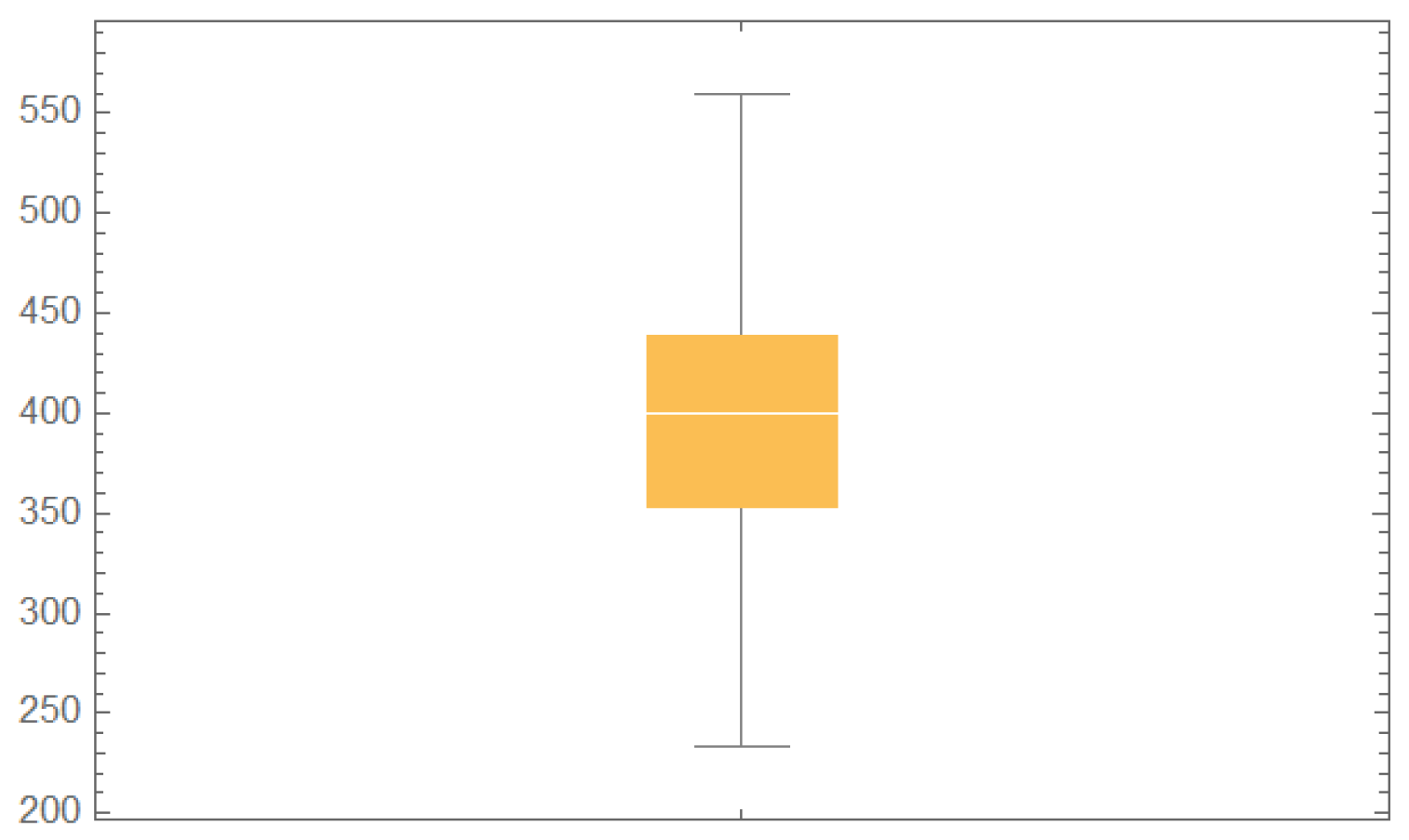
Descriptive statistics of these data are presented in Table 12.
Based on the descriptive statistics in Table 12, we observed that the skewness value was close to zero; thus, the distribution of the fatigue life of the 6061-T6 aluminum coupons’ cut dataset was approximately normal, while the variance was 3884.30, which indicate high variability in the dataset.
According to Figure 1, we can note that there were no outliers in the fatigue life of the 6061-T6 aluminum coupons’ cut data. The ML estimates and Bayesian estimates via the standard Bayes technique of the BIED parameters for the fatigue life of the 6061-T6 aluminum coupons’ cut data are presented in Table 13 at two censoring percentages of and .
The ML estimates of the model parameters and the performance of the BIED against other models for the fatigue life of the 6061-T6 aluminum coupons’ cut data are presented in Table 14 at two censoring percentages of and .
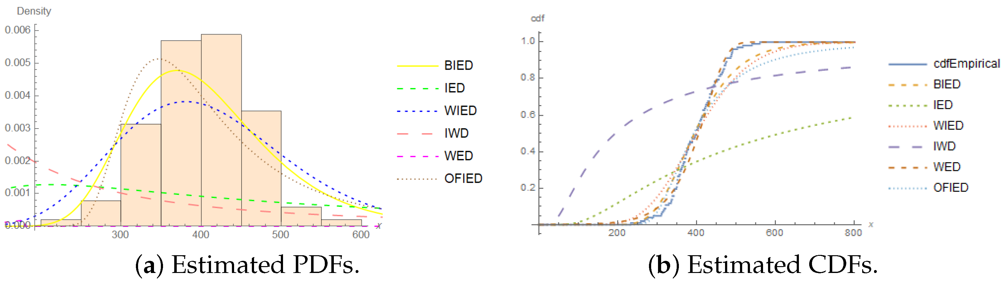
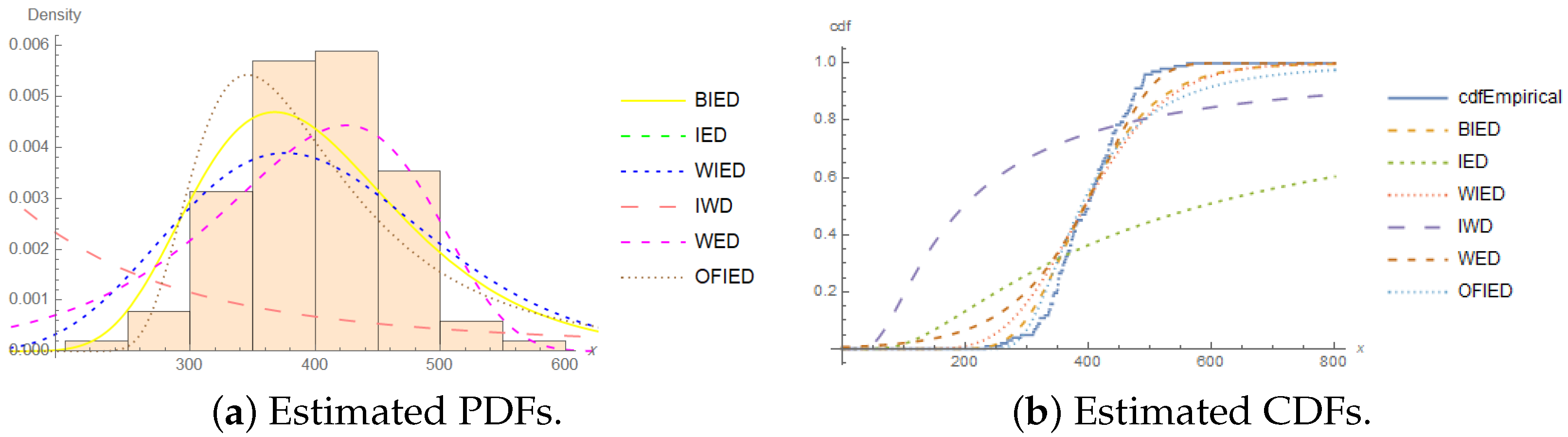
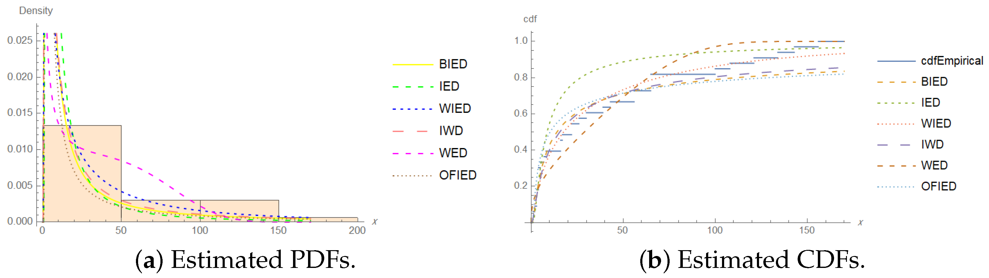
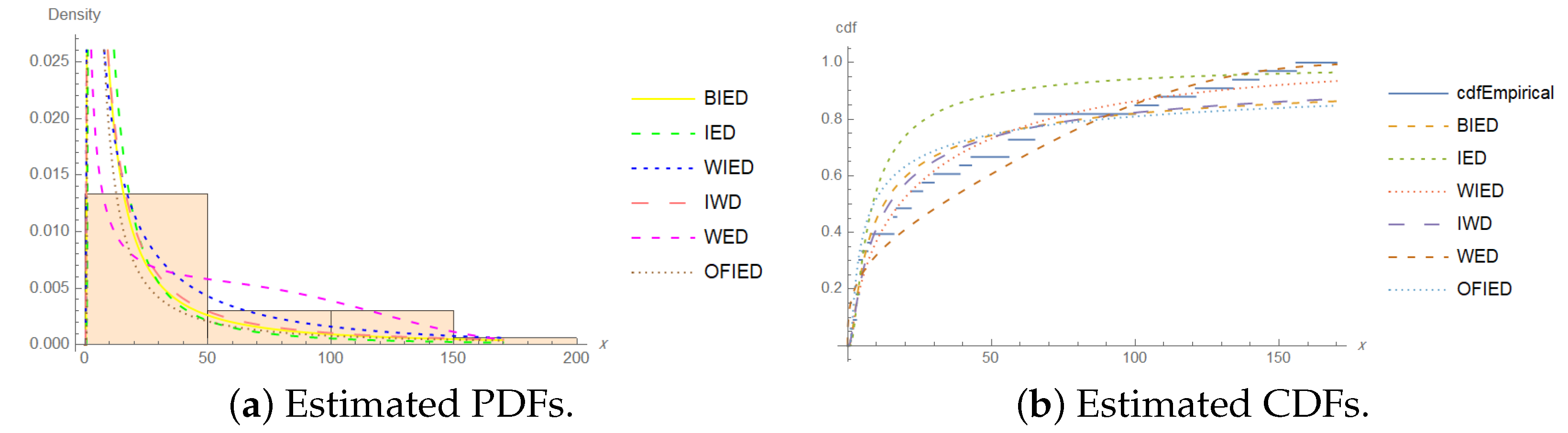
In Table 14, the values of the AIC, BIC, CAIC, and HQIC show that the BIED was the best model for analyzing the fatigue life of the 6061-T6 aluminum coupons’ cut data. Furthermore, we can consider that the WED is a good alternative model for these data. The estimated PDF and estimated CDF of the models for the fatigue life of the 6061-T6 aluminum coupons’ cut data at two censoring percentages of and are shown in Figure 2 and Figure 3.
- Patients suffering from acute myelogenous leukemia:
The following data consisting of 33 observations were studied by Feigl and Zelen [22] and represent the survival times (in weeks) of patients suffering from acute myelogenous leukemia.
- 1, 1, 2, 3, 3, 3, 4, 4, 4, 4, 5, 7, 8, 16, 16, 17, 22, 22, 26, 30,39, 43, 56, 56, 65, 65, 65, 100, 108, 121, 134, 143, 156
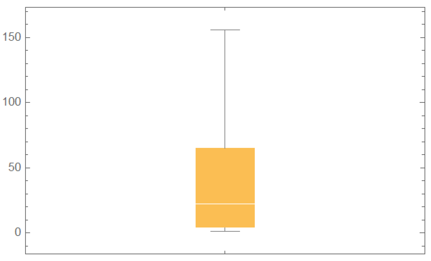
Descriptive statistics of these data are presented in Table 15.
According to the descriptive statistics in Table 15, we observed that the distribution of the survival times (in weeks) of patients suffering from acute myelogenous leukemia data was positively skewed, while the variance was 2181.17, which indicates high variability in the dataset.
According to Figure 4, we can note that there were no outliers in the survival times (in weeks) of patients suffering from acute myelogenous leukemia data. Additionally, the ML estimates and Bayesian estimates via the standard Bayes technique of the BIED for this dataset are presented in Table 16 at two censoring percentages of and .
The ML estimates of the model parameters and the performance of the BIED against other models for the survival times (in weeks) of patients suffering from acute myelogenous leukemia data are shown in Table 14 at two censoring percentages of and .
Table 17, based on the values of the AIC, BIC, CAIC, and HQIC, shows that the BIED was the best model for fitting the survival times (in weeks) of patients suffering from acute myelogenous leukemia data. Further, the estimated PDF and estimated CDF of the models for this dataset at two censoring percentages of and are shown in Figure 5 and Figure 6.
5. Conclusions
In this article, the maximum likelihood and Bayes estimators of the BIED were derived based on type-II censored samples. The invariance property was used to estimate the survival and hazard functions. Furthermore, in the Bayesian estimation, three loss functions were used with two techniques. The gamma distribution was assumed as a prior distribution for the shape and scale parameters. Besides, it can be concluded that the MSEs of the ML estimates and Bayes estimates for the unknown parameters decreased as the sample size increased. Furthermore, when was unknown, the Bayes estimates gave better estimates via the standard Bayes technique. The ML estimates gave better estimates than the Bayes estimates using the two techniques when was unknown. For the third case, when was unknown, the ML estimates gave better results than the Bayes estimates as the sample size increased. Likewise, when and were unknown, the Bayes estimates via the importance sampling technique under the LINEX loss function () gave better results than the ML estimates as the sample size increased. Two real datasets were applied, and the BIED provided a better fit than the other compared distributions.
Author Contributions
Software, L.S.A.; supervision and writing—review, R.A.B. and M.A.A.; methodology and writing—original draft, L.S.A. All authors have read and agreed to the published version of the manuscript.
Funding
This research received no external funding.
Institutional Review Board Statement
Not applicable.
Informed Consent Statement
Not applicable.
Data Availability Statement
Not applicable.
Conflicts of Interest
The authors declare no conflict of interest.
References
- Singh, U.; Gupta, P.K.; Upadhyay, S.K. Estimation of parameters for exponentiated Wibull family under type-II censoring scheme. Comput. Stat. Data Anal. 2005, 48, 509–523. [Google Scholar] [CrossRef]
- Prakash, G. Some estimation procedures for the inverted exponential distribution. S. Pac. J. Nat. Appl. Sci. 2009, 27, 71–78. [Google Scholar] [CrossRef] [Green Version]
- Dey, S.; Dey, T. On progressively censored generalized inverted exponential distribution. J. Appl. Stat. 2014, 41, 2557–2576. [Google Scholar] [CrossRef]
- Singh, B.; Goel, R. The beta inverted exponential distribution: Properties and applications. Int. J. Appl. Sci. Math. 2015, 2, 132–141. [Google Scholar]
- Garg, R.; Dube, M.; Kumar, K.; Krishna, H. On randomly censored generalized inverted exponential distribution. Am. J. Math. Manag. Sci. 2016, 35, 361–379. [Google Scholar] [CrossRef]
- Bakoban, R.; Abu-Zinadah, H.H. The beta generalized inverted exponential distribution with real data applications. REVSTAT-Stat. J. 2017, 15, 65–88. [Google Scholar]
- Aldahlan, M.A. The inverse Weibull inverse exponential distribution with application. Int. J. Contemp. Math. Sci. 2019, 14, 17–30. [Google Scholar] [CrossRef] [Green Version]
- Arnold, B.C.; Balakrishnan, N.; Nagaraja, H.N. A First Course in Order Statistics; Society for Industrial and Applied Mathematics: Philadelphia, PA, USA, 2008. [Google Scholar]
- Abramowitz, M.; Stegun, I.A. Handbook of Mathematical Functions with Formulas, Graphs, and Mathematical Tables, 2nd ed.; Dover Publication: New York, NY, USA, 1972. [Google Scholar]
- Olver, F.W.; Lozier, D.W.; Boisvert, R.F.; Clark, C.W. NIST Handbook of Mathematical Functions, 1st ed.; Cambridge University Press: New York, NY, USA, 2010. [Google Scholar]
- Box, G.E.; Tiao, G.C. Bayesian Inference in Statistical Analysis, 1st ed.; John Wiley & Sons: Hoboken, NJ, USA, 1992. [Google Scholar]
- Varian, H.R. A Bayesian approach to real estate assessment. Stud. Bayesian Econom. Stat. Honor. Leonard J. Savage 1975, 5, 195–208. [Google Scholar]
- Calabria, R.; Pulcini, G. An engineering approach to Bayes estimation for the Weibull distribution. Microelectron. Reliab. 1994, 34, 789–802. [Google Scholar] [CrossRef]
- Lin, C.; Duran, B.; Lewis, T. Inverted gamma as a life distribution. Microelectron. Reliab. 1989, 29, 619–626. [Google Scholar] [CrossRef]
- Keller, A.Z.; Kamath, A.R.R. Alternate reliability models for mechanical systems. In Proceedings of the 3rd International Conference on Reliability and Maintainability, Toulouse, France, 18–21 October 1982; pp. 411–415. [Google Scholar]
- Pelumi, E.O.; Adebowale, O.A.; Enahoro, A.O. The Weibull inverted exponential distribution: A generalization of the inverse exponential distribution. In Proceedings of the World Congress on Engineering, London, UK, 5–7 July 2017; Volume 1, pp. 16–19. [Google Scholar]
- Oguntunde, P.; Balogun, O.; Okagbue, H.; Bishop, S. The Weibull exponential distribution: Its properties and applications. J. Appl. Sci. 2015, 15, 1305–1311. [Google Scholar] [CrossRef]
- Alrajhi, S. The odd Fréchet inverse exponential distribution with application. J. Nonlinear Sci. Appl. 2019, 12, 535–542. [Google Scholar] [CrossRef] [Green Version]
- Christie, M.; Cliffe, A.; Dawid, P.; Senn, S.S. Simplicity, Complexity and Modelling; John Wiley & Sons: Hoboken, NJ, USA, 2011. [Google Scholar]
- Hannan, E.J.; Quinn, B.G. The determination of the order of an autoregression. J. R. Stat. Soc. 1979, 41, 190–195. [Google Scholar] [CrossRef]
- Birnbaum, Z.W.; Saunders, S.C. Estimation for a family of life distributions with applications to fatigue. J. Appl. Probab. 1969, 6, 328–347. [Google Scholar] [CrossRef]
- Feigl, P.; Zelen, M. Estimation of exponential survival probabilities with concomitant information. Biometrics 1965, 21, 826–838. [Google Scholar] [CrossRef] [PubMed]
Figure 1.
Boxplot for the fatigue life of the 6061-T6 aluminum coupons’ cut data.

Figure 2.
Plots of the estimated PDF and estimated CDF of the models for the fatigue life of the 6061-T6 aluminum coupons’ cut data for .
Figure 2.
Plots of the estimated PDF and estimated CDF of the models for the fatigue life of the 6061-T6 aluminum coupons’ cut data for .

Figure 3.
Plots of the estimated PDF and estimated CDF of the models for the fatigue life of the 6061-T6 aluminum coupons’ cut data for .
Figure 3.
Plots of the estimated PDF and estimated CDF of the models for the fatigue life of the 6061-T6 aluminum coupons’ cut data for .

Figure 4.
Boxplot for the survival times (in weeks) of patients suffering from acute myelogenous leukemia data.
Figure 4.
Boxplot for the survival times (in weeks) of patients suffering from acute myelogenous leukemia data.

Figure 5.
Plots of the estimated PDF and estimated CDF of the models for the patients suffering from acute myelogenous leukemia data for .
Figure 5.
Plots of the estimated PDF and estimated CDF of the models for the patients suffering from acute myelogenous leukemia data for .

Figure 6.
Plots of the estimated PDF and estimated CDF of the models for the patients suffering from acute myelogenous leukemia data for .
Figure 6.
Plots of the estimated PDF and estimated CDF of the models for the patients suffering from acute myelogenous leukemia data for .


Table 1.
The ML estimates, bias, and MSE of the parameters , , , and for true parameter values (, , ).
Table 1.
The ML estimates, bias, and MSE of the parameters , , , and for true parameter values (, , ).
| n | r | ||||||
|---|---|---|---|---|---|---|---|
| 30 | 24 | MLE | 1.27791 | 4.05604 | 2.45134 | 0.73519 | 0.83076 |
| Bias | 0.47791 | 0.05604 | −0.54866 | 0.00615 | 0.01291 | ||
| MSE | 0.65026 | 1.07637 | 0.82283 | 0.00402 | 0.02662 | ||
| 27 | MLE | 0.89924 | 4.01143 | 2.85928 | 0.72555 | 0.82323 | |
| Bias | 0.09924 | 0.01143 | −0.14072 | −0.00349 | 0.00537 | ||
| MSE | 0.07609 | 0.92676 | 0.32039 | 0.00396 | 0.02497 | ||
| 50 | 40 | MLE | 0.88102 | 3.97067 | 2.90404 | 0.73132 | 0.81202 |
| Bias | 0.08102 | −0.02934 | −0.09596 | 0.00227 | −0.00584 | ||
| MSE | 0.05673 | 0.28639 | 0.20724 | 0.00250 | 0.01299 | ||
| 45 | MLE | 0.87403 | 3.95937 | 2.90266 | 0.73291 | 0.80861 | |
| Bias | 0.07403 | −0.04063 | −0.09734 | 0.00386 | −0.00925 | ||
| MSE | 0.03969 | 0.27514 | 0.19996 | 0.00258 | 0.01454 | ||
| 100 | 80 | MLE | 0.86352 | 3.99116 | 2.92567 | 0.73380 | 0.80855 |
| Bias | 0.06352 | −0.00884 | −0.07433 | 0.00475 | −0.00931 | ||
| MSE | 0.03542 | 0.22032 | 0.13827 | 0.00131 | 0.00643 | ||
| 90 | MLE | 0.84168 | 3.98337 | 2.96389 | 0.73189 | 0.81021 | |
| Bias | 0.04168 | −0.01664 | −0.03611 | 0.00285 | −0.00765 | ||
| MSE | 0.02752 | 0.20084 | 0.15640 | 0.00134 | 0.00786 | ||
Table 2.
The ML estimates, bias, and MSE of the parameters , , and for true parameter values .
| n | r | ||||||
|---|---|---|---|---|---|---|---|
| 30 | 24 | MLE | 3.28695 | 0.88241 | 3.08763 | 0.87765 | 0.05352 |
| Bias | 0.28695 | 0.08241 | 0.08763 | 0.00161 | −0.00000 | ||
| MSE | 0.96247 | 0.04896 | 0.18824 | 0.00214 | 0.00020 | ||
| 27 | MLE | 3.20203 | 0.87913 | 3.07017 | 0.87230 | 0.05497 | |
| Bias | 0.20203 | 0.07913 | 0.07017 | −0.00374 | 0.00144 | ||
| MSE | 0.86952 | 0.04667 | 0.15728 | 0.00203 | 0.00017 | ||
| 50 | 40 | MLE | 3.17675 | 0.86190 | 3.02640 | 0.87315 | 0.05506 |
| Bias | 0.17675 | 0.06191 | 0.02631 | −0.00288 | 0.00154 | ||
| MSE | 0.52161 | 0.02995 | 0.10801 | 0.00132 | 0.00012 | ||
| 45 | MLE | 3.09316 | 0.84395 | 3.04172 | 0.87372 | 0.05457 | |
| Bias | 0.09316 | 0.04395 | 0.04172 | −0.00232 | 0.00104 | ||
| MSE | 0.33268 | 0.02347 | 0.08888 | 0.00102 | 0.00009 | ||
| 100 | 80 | MLE | 3.09505 | 0.83487 | 3.02198 | 0.87445 | 0.05438 |
| Bias | 0.09504 | 0.03487 | 0.02198 | −0.00159 | 0.00086 | ||
| MSE | 0.25649 | 0.01383 | 0.07476 | 0.00077 | 0.00006 | ||
| 90 | MLE | 3.09843 | 0.82840 | 3.02111 | 0.87805 | 0.05333 | |
| Bias | 0.09843 | 0.02839 | 0.02111 | 0.00201 | −0.00020 | ||
| MSE | 0.14981 | 0.01212 | 0.05592 | 0.00046 | 0.00003 | ||
Table 3.
The ML estimates, bias, and MSE of the parameters , , and for true parameter values .
| n | r | ||||||
|---|---|---|---|---|---|---|---|
| 30 | 24 | MLE | 3.76231 | 8.04103 | 1.83068 | 0.22896 | 1.62124 |
| Bias | 0.76231 | 0.04103 | −0.16932 | 0.00425 | 0.01296 | ||
| MSE | 2.04744 | 0.26625 | 0.17399 | 0.00279 | 0.02465 | ||
| 27 | MLE | 3.71919 | 7.99749 | 1.84219 | 0.23080 | 1.61052 | |
| Bias | 0.71919 | −0.00251 | −0.15782 | 0.00609 | 0.00224 | ||
| MSE | 2.04687 | 0.29352 | 0.16868 | 0.00289 | 0.02392 | ||
| 50 | 40 | MLE | 3.26032 | 7.98509 | 1.93754 | 0.22686 | 1.60902 |
| Bias | 0.26032 | −0.01491 | −0.06246 | 0.00215 | 0.00074 | ||
| MSE | 0.59433 | 0.21877 | 0.07295 | 0.00142 | 0.01337 | ||
| 45 | MLE | 3.27549 | 7.95998 | 1.93706 | 0.22960 | 1.59955 | |
| Bias | 0.27549 | −0.04002 | −0.06294 | 0.00489 | −0.00873 | ||
| MSE | 0.61335 | 0.20042 | 0.07451 | 0.00132 | 0.01260 | ||
| 100 | 80 | MLE | 3.17247 | 7.97533 | 1.97010 | 0.23002 | 1.59641 |
| Bias | 0.17247 | −0.02467 | −0.02990 | 0.00531 | −0.01187 | ||
| MSE | 0.41601 | 0.17126 | 0.05337 | 0.00072 | 0.00807 | ||
| 90 | MLE | 3.18983 | 7.98382 | 1.95748 | 0.22795 | 1.60322 | |
| Bias | 0.18983 | −0.01618 | −0.04253 | 0.00324 | −0.00506 | ||
| MSE | 0.39486 | 0.16581 | 0.04962 | 0.00068 | 0.00795 | ||
Table 4.
The four cases for calculating the Bayes estimators via the standard Bayes and importance sampling techniques.
Table 4.
The four cases for calculating the Bayes estimators via the standard Bayes and importance sampling techniques.
| Case 1 When Is Unknown | Case 2 When Is Unknown | |
|---|---|---|
| standard Bayes technique | The Bayes estimates of under SE, LINEX, and GE are obtained by computing Equations (25), (27) and (29). | The Bayes estimates of are obtained numerically under the SE, LINEX, and GE loss functions by evaluating (38), (39) and (40), respectively. |
| importance sampling technique | According to Algorithm 1, the Bayes estimates of are obtained under the SE, LINEX, and GE loss functions by computing Equations (31), (32) and (33), respectively. | Based on Algorithm 2, the Bayes estimates of are obtained numerically by computing Equations (42)–(44) under three loss functions. |
| Case 3 When Is Unknown | Case 4 When andAre Unknown | |
| standard Bayes technique | The Bayes estimates of are obtained under the SE, LINEX, and GE loss functions by evaluating (49), (50) and (51), respectively. | — |
| importance sampling technique | Based on Algorithm 3, the Bayes estimates of are obtained numerically by computing Equations (53)–(55) under three loss functions. | The Bayes estimates of are obtained numerically according to Algorithm 4 under the SE, LINEX, and GE loss functions by computing Equations (70), (71) and (72), respectively. |
Table 5.
The ML and Bayesian estimates of the unknown parameters , , and via the standard Bayes technique.
Table 5.
The ML and Bayesian estimates of the unknown parameters , , and via the standard Bayes technique.
| n | r | Parameters | ML Estimates | Bayes Estimates | |||||||
|---|---|---|---|---|---|---|---|---|---|---|---|
| SE | LINEX | GE | |||||||||
| 30 | 24 | Mean | 0.81865 | 0.78855 | 0.78855 | 0.77828 | 0.76692 | 0.78855 | 0.75448 | 0.82343 | |
| Bias | 0.01865 | −0.01148 | −0.01148 | −0.02172 | −0.03308 | −0.01148 | −0.04552 | 0.02343 | |||
| MSE | 0.01887 | 0.01353 | 0.01353 | 0.01362 | 0.01343 | 0.01353 | 0.01516 | 0.01556 | |||
| Mean | 0.73107 | 0.71139 | 0.71139 | 0.70988 | 0.70922 | 0.71139 | 0.70186 | 0.72454 | |||
| Bias | 0.00203 | −0.01766 | −0.01766 | −0.01916 | −0.01982 | −0.01766 | −0.02718 | −0.00450 | |||
| MSE | 0.00426 | 0.00362 | 0.00362 | 0.00384 | 0.00401 | 0.00362 | 0.00443 | 0.00340 | |||
| Mean | 0.80731 | 0.84351 | 0.84351 | 0.82278 | 0.78846 | 0.84351 | 0.79688 | 0.84694 | |||
| Bias | −0.01055 | 0.02566 | 0.02566 | 0.00492 | −0.02940 | 0.02566 | −0.02098 | 0.02908 | |||
| MSE | 0.01848 | 0.01440 | 0.01440 | 0.01443 | 0.01570 | 0.01440 | 0.01665 | 0.01468 | |||
| 27 | Mean | 0.81917 | 0.79216 | 0.79216 | 0.78044 | 0.76701 | 0.79216 | 0.75675 | 0.82325 | ||
| Bias | 0.01917 | −0.00784 | −0.00784 | −0.01956 | −0.03299 | −0.00784 | −0.04325 | 0.02325 | |||
| MSE | 0.01834 | 0.01359 | 0.01359 | 0.01385 | 0.01359 | 0.01359 | 0.01528 | 0.01574 | |||
| Mean | 0.73155 | 0.71345 | 0.71345 | 0.71092 | 0.70921 | 0.71345 | 0.70296 | 0.72447 | |||
| Bias | 0.00250 | −0.01559 | −0.01559 | −0.01813 | −0.01983 | −0.01559 | −0.02608 | −0.00457 | |||
| MSE | 0.00415 | 0.00355 | 0.00355 | 0.00386 | 0.00398 | 0.00355 | 0.00443 | 0.00336 | |||
| Mean | 0.80652 | 0.83954 | 0.83954 | 0.82074 | 0.78878 | 0.83954 | 0.79485 | 0.84697 | |||
| Bias | −0.01133 | 0.02168 | 0.02168 | 0.00288 | −0.02908 | 0.02168 | −0.02300 | 0.02911 | |||
| MSE | 0.01797 | 0.01425 | 0.01425 | 0.01469 | 0.01562 | 0.01425 | 0.01704 | 0.01467 | |||
| 50 | 40 | Mean | 0.81429 | 0.80057 | 0.80057 | 0.77973 | 0.78116 | 0.80057 | 0.76534 | 0.81616 | |
| Bias | 0.01429 | 0.00057 | 0.00057 | −0.02028 | −0.01884 | 0.00057 | −0.03466 | 0.01616 | |||
| MSE | 0.01037 | 0.00853 | 0.00853 | 0.00917 | 0.00878 | 0.00853 | 0.00994 | 0.00976 | |||
| Mean | 0.73215 | 0.72202 | 0.72202 | 0.71340 | 0.71759 | 0.72202 | 0.70869 | 0.72696 | |||
| Bias | 0.00311 | −0.00702 | −0.00702 | −0.01564 | −0.01146 | −0.00702 | −0.02035 | −0.00209 | |||
| MSE | 0.00241 | 0.00218 | 0.00218 | 0.00258 | 0.00246 | 0.00218 | 0.00282 | 0.00223 | |||
| Mean | 0.80789 | 0.82577 | 0.82577 | 0.82830 | 0.79768 | 0.82577 | 0.81316 | 0.83430 | |||
| Bias | −0.00997 | 0.00791 | 0.00791 | 0.01045 | −0.02017 | 0.00791 | −0.00469 | 0.01644 | |||
| MSE | 0.01043 | 0.00897 | 0.00897 | 0.00974 | 0.01006 | 0.00897 | 0.01035 | 0.00950 | |||
| 45 | Mean | 0.81224 | 0.80057 | 0.80057 | 0.78936 | 0.78158 | 0.80057 | 0.77503 | 0.81643 | ||
| Bias | 0.01224 | 0.00057 | 0.00057 | −0.01064 | −0.01842 | 0.00057 | −0.02497 | 0.01643 | |||
| MSE | 0.01046 | 0.00853 | 0.00853 | 0.00919 | 0.00860 | 0.00853 | 0.00969 | 0.00958 | |||
| Mean | 0.73105 | 0.72202 | 0.72202 | 0.71835 | 0.71788 | 0.72202 | 0.71375 | 0.72721 | |||
| Bias | 0.00201 | −0.00702 | −0.00702 | −0.01069 | −0.01116 | −0.00702 | −0.01529 | −0.00184 | |||
| MSE | 0.00249 | 0.00218 | 0.00218 | 0.00243 | 0.00238 | 0.00218 | 0.00263 | 0.00216 | |||
| Mean | 0.81007 | 0.82577 | 0.82577 | 0.81829 | 0.79734 | 0.82577 | 0.80287 | 0.83380 | |||
| Bias | −0.00779 | 0.00791 | 0.00791 | 0.00044 | −0.02052 | 0.00791 | −0.01498 | 0.01594 | |||
| MSE | 0.01066 | 0.00897 | 0.00897 | 0.00972 | 0.00982 | 0.00897 | 0.01066 | 0.00925 | |||
| 100 | 80 | Mean | 0.80413 | 0.79939 | 0.79939 | 0.79528 | 0.78855 | 0.79939 | 0.78803 | 0.80636 | |
| Bias | 0.00413 | −0.00061 | −0.00061 | −0.00472 | −0.01145 | −0.00061 | −0.01197 | 0.00636 | |||
| MSE | 0.00506 | 0.00468 | 0.00468 | 0.00454 | 0.00476 | 0.00468 | 0.00466 | 0.00496 | |||
| Mean | 0.72907 | 0.72486 | 0.72486 | 0.72400 | 0.72220 | 0.72486 | 0.72176 | 0.72698 | |||
| Bias | 0.00003 | −0.00419 | −0.00419 | −0.00504 | −0.00684 | −0.00419 | −0.00728 | −0.00207 | |||
| MSE | 0.00126 | 0.00119 | 0.00119 | 0.00118 | 0.00128 | 0.00119 | 0.00123 | 0.00121 | |||
| Mean | 0.81597 | 0.82298 | 0.82298 | 0.81716 | 0.80936 | 0.82298 | 0.80948 | 0.82824 | |||
| Bias | −0.00189 | 0.00512 | 0.00512 | −0.00079 | −0.00849 | 0.00512 | −0.00837 | 0.01038 | |||
| MSE | 0.00532 | 0.00497 | 0.00497 | 0.00485 | 0.00523 | 0.00497 | 0.00509 | 0.00514 | |||
| 90 | Mean | 0.80925 | 0.79939 | 0.79939 | 0.78986 | 0.79195 | 0.79939 | 0.78264 | 0.80978 | ||
| Bias | 0.00925 | −0.00061 | −0.00061 | −0.01014 | −0.00805 | −0.00061 | −0.01736 | 0.00981 | |||
| MSE | 0.00558 | 0.00468 | 0.00468 | 0.00443 | 0.00428 | 0.00468 | 0.00463 | 0.00458 | |||
| Mean | 0.73148 | 0.72486 | 0.72486 | 0.72129 | 0.72414 | 0.72486 | 0.71903 | 0.72887 | |||
| Bias | 0.00244 | −0.00419 | −0.00419 | −0.00775 | −0.00490 | −0.00419 | −0.01001 | −0.00017 | |||
| MSE | 0.00134 | 0.00119 | 0.00119 | 0.00117 | 0.00115 | 0.00119 | 0.00123 | 0.00110 | |||
| Mean | 0.81088 | 0.82298 | 0.82298 | 0.82279 | 0.80565 | 0.82298 | 0.81525 | 0.82449 | |||
| Bias | −0.00698 | 0.00512 | 0.00512 | 0.00494 | −0.01221 | 0.00512 | −0.00261 | 0.00663 | |||
| MSE | 0.00574 | 0.00497 | 0.00497 | 0.00468 | 0.00486 | 0.00497 | 0.00483 | 0.00464 | |||
Table 6.
The ML and Bayesian estimates of the unknown parameters , , and via the importance sampling technique.
Table 6.
The ML and Bayesian estimates of the unknown parameters , , and via the importance sampling technique.
| n | r | Parameters | ML Estimates | Bayes Estimates | |||||||
|---|---|---|---|---|---|---|---|---|---|---|---|
| SE | LINEX | GE | |||||||||
| 30 | 24 | Mean | 0.81865 | 1.67661 | 1.67661 | 1.67045 | 1.67654 | 1.67661 | 1.67018 | 1.68018 | |
| Bias | 0.01865 | 0.87661 | 0.87661 | 0.87045 | 0.87654 | 0.87661 | 0.87018 | 0.88018 | |||
| MSE | 0.01887 | 0.80599 | 0.80599 | 0.79622 | 0.80872 | 0.80599 | 0.79580 | 0.81512 | |||
| Mean | 0.73107 | 0.95051 | 0.95051 | 0.94989 | 0.95050 | 0.95051 | 0.94988 | 0.95056 | |||
| Bias | 0.00203 | 0.22147 | 0.22147 | 0.22085 | 0.22146 | 0.22147 | 0.22083 | 0.22152 | |||
| MSE | 0.00426 | 0.04944 | 0.04944 | 0.04917 | 0.04946 | 0.04944 | 0.04917 | 0.04948 | |||
| Mean | 0.80731 | 0.23678 | 0.23678 | 0.23875 | 0.23595 | 0.23678 | 0.23778 | 0.23714 | |||
| Bias | −0.01055 | −0.58108 | −0.58108 | −0.57910 | −0.58190 | −0.58108 | −0.58008 | −0.58072 | |||
| MSE | 0.01848 | 0.34284 | 0.34284 | 0.34064 | 0.34411 | 0.34284 | 0.34175 | 0.34278 | |||
| 27 | Mean | 0.81917 | 1.59218 | 1.59218 | 1.58224 | 1.58460 | 1.59218 | 1.58198 | 1.58762 | ||
| Bias | 0.01917 | 0.79218 | 0.79218 | 0.78224 | 0.78460 | 0.79218 | 0.78198 | 0.78726 | |||
| MSE | 0.01834 | 0.66092 | 0.66092 | 0.64575 | 0.652221 | 0.66092 | 0.64539 | 0.65639 | |||
| Mean | 0.73155 | 0.94133 | 0.94133 | 0.94017 | 0.94019 | 0.94133 | 0.94015 | 0.94024 | |||
| Bias | 0.00250 | 0.21228 | 0.21228 | 0.21112 | 0.21114 | 0.21228 | 0.21110 | 0.21120 | |||
| MSE | 0.00415 | 0.04553 | 0.04553 | 0.04505 | 0.04514 | 0.04553 | 0.04504 | 0.04516 | |||
| Mean | 0.80652 | 0.26985 | 0.26985 | 0.27369 | 0.27273 | 0.26985 | 0.27290 | 0.27374 | |||
| Bias | −0.01133 | −0.54800 | −0.54800 | −0.54417 | −0.54512 | −0.54800 | −0.54496 | −0.54412 | |||
| MSE | 0.01797 | 0.30597 | 0.30597 | 0.30183 | 0.30362 | 0.30597 | 0.30268 | 0.30258 | |||
| 50 | 40 | Mean | 0.81429 | 1.02888 | 1.02888 | 1.02199 | 1.02842 | 1.02888 | 1.02189 | 1.02878 | |
| Bias | 0.01429 | 0.22888 | 0.22888 | 0.22199 | 0.22842 | 0.22888 | 0.22189 | 0.22879 | |||
| MSE | 0.01037 | 0.06184 | 0.06184 | 0.05813 | 0.06164 | 0.06184 | 0.05809 | 0.06180 | |||
| Mean | 0.73215 | 0.82255 | 0.82255 | 0.82034 | 0.82241 | 0.82255 | 0.82032 | 0.82245 | |||
| Bias | 0.00311 | 0.09350 | 0.09350 | 0.09130 | 0.09337 | 0.09350 | 0.09128 | 0.09342 | |||
| MSE | 0.00241 | 0.00982 | 0.00982 | 0.00938 | 0.00984 | 0.00982 | 0.00937 | 0.00985 | |||
| Mean | 0.80789 | 0.60854 | 0.60854 | 0.61387 | 0.60854 | 0.60854 | 0.61373 | 0.60884 | |||
| Bias | −0.00997 | −0.20932 | −0.20932 | −0.20399 | −0.20932 | −0.20932 | −0.20413 | −0.20902 | |||
| MSE | 0.01043 | 0.05011 | 0.05011 | 0.04761 | 0.05025 | 0.05011 | 0.04767 | 0.05014 | |||
| 45 | Mean | 0.81224 | 1.01755 | 1.01755 | 1.01760 | 1.01795 | 1.01755 | 1.01750 | 1.01824 | ||
| Bias | 0.01224 | 0.21755 | 0.21755 | 0.21760 | 0.21795 | 0.21755 | 0.21750 | 0.21824 | |||
| MSE | 0.01046 | 0.05601 | 0.05601 | 0.05580 | 0.05697 | 0.05601 | 0.05577 | 0.05709 | |||
| Mean | 0.73105 | 0.81880 | 0.81880 | 0.81891 | 0.81874 | 0.81880 | 0.81889 | 0.81878 | |||
| Bias | 0.00201 | 0.08976 | 0.08976 | 0.08986 | 0.08970 | 0.08976 | 0.08984 | 0.08974 | |||
| MSE | 0.00249 | 0.00909 | 0.00909 | 0.00909 | 0.00920 | 0.00909 | 0.00909 | 0.00920 | |||
| Mean | 0.81007 | 0.61768 | 0.61768 | 0.61741 | 0.61736 | 0.61768 | 0.61728 | 0.61761 | |||
| Bias | −0.00779 | −0.20017 | −0.20017 | −0.20045 | −0.20050 | −0.20017 | −0.20058 | −0.20025 | |||
| MSE | 0.01066 | 0.04604 | 0.04604 | 0.04599 | 0.04675 | 0.04604 | 0.04603 | 0.04666 | |||
| 100 | 80 | Mean | 0.80413 | 0.64656 | 0.64656 | 0.64757 | 0.64685 | 0.64656 | 0.64756 | 0.64688 | |
| Bias | 0.00413 | −0.15344 | −0.15344 | −0.15243 | −0.15315 | −0.15344 | −0.15245 | −0.15312 | |||
| MSE | 0.00506 | 0.02546 | 0.02546 | 0.02526 | 0.02531 | 0.02546 | 0.02527 | 0.02530 | |||
| Mean | 0.72907 | 0.64000 | 0.64000 | 0.64060 | 0.64022 | 0.64000 | 0.64059 | 0.64024 | |||
| Bias | 0.00003 | −0.08904 | −0.08904 | −0.08844 | −0.08882 | −0.08904 | −0.08845 | −0.08880 | |||
| MSE | 0.00126 | 0.00872 | 0.00872 | 0.00865 | 0.00865 | 0.00872 | 0.00865 | 0.00865 | |||
| Mean | 0.81597 | 0.98945 | 0.98945 | 0.98829 | 0.98903 | 0.98945 | 0.98828 | 0.98906 | |||
| Bias | −0.00189 | 0.17159 | 0.17159 | 0.17043 | 0.17117 | 0.17159 | 0.17042 | 0.17120 | |||
| MSE | 0.00532 | 0.03213 | 0.03213 | 0.03187 | 0.03189 | 0.03213 | 0.03187 | 0.03190 | |||
| 90 | Mean | 0.80925 | 0.65127 | 0.65127 | 0.65130 | 0.64958 | 0.65127 | 0.65128 | 0.64961 | ||
| Bias | 0.00925 | −0.14873 | −0.14873 | −0.14871 | −0.15042 | −0.14873 | −0.14872 | −0.15039 | |||
| MSE | 0.00558 | 0.02400 | 0.02400 | 0.02392 | 0.02447 | 0.02400 | 0.02392 | 0.02446 | |||
| Mean | 0.73148 | 0.64305 | 0.64305 | 0.64310 | 0.64198 | 0.64305 | 0.64309 | 0.64199 | |||
| Bias | 0.00244 | −0.08560 | −0.08560 | −0.08594 | −0.08706 | −0.08560 | −0.08595 | −0.08705 | |||
| MSE | 0.00134 | 0.00815 | 0.00815 | 0.00812 | 0.00834 | 0.00815 | 0.00812 | 0.00833 | |||
| Mean | 0.81088 | 0.98385 | 0.98385 | 0.98377 | 0.98579 | 0.98385 | 0.98376 | 0.98583 | |||
| Bias | −0.00698 | 0.16599 | 0.16599 | 0.16592 | 0.16794 | 0.16599 | 0.16591 | 0.16797 | |||
| MSE | 0.00574 | 0.03015 | 0.03015 | 0.03003 | 0.03078 | 0.03015 | 0.03003 | 0.03079 | |||
Table 7.
The ML and Bayesian estimates of the unknown parameters , , and via the standard Bayes technique.
Table 7.
The ML and Bayesian estimates of the unknown parameters , , and via the standard Bayes technique.
| n | r | Parameters | ML Estimates | Bayes Estimates | |||||||
|---|---|---|---|---|---|---|---|---|---|---|---|
| SE | LINEX | GE | |||||||||
| 30 | 24 | Mean | 4.00137 | 3.63379 | 3.63379 | 3.21065 | 2.75023 | 3.63379 | 3.37739 | 3.84007 | |
| Bias | 0.00137 | −0.36621 | −0.36621 | −0.78935 | −1.24977 | −0.36621 | −0.62261 | −0.15993 | |||
| MSE | 0.52494 | 0.47324 | 0.47324 | 0.82890 | 1.66793 | 0.47324 | 0.68487 | 0.38669 | |||
| Mean | 0.73031 | 0.74993 | 0.74993 | 0.74633 | 0.74334 | 0.74993 | 0.74383 | 0.74885 | |||
| Bias | 0.00126 | 0.02089 | 0.02089 | 0.01729 | 0.01429 | 0.02089 | 0.01479 | 0.01981 | |||
| MSE | 0.00130 | 0.00130 | 0.00130 | 0.00121 | 0.00109 | 0.00130 | 0.00117 | 0.00121 | |||
| Mean | 0.81692 | 0.74893 | 0.74893 | 0.73874 | 0.71619 | 0.74893 | 0.70815 | 0.78359 | |||
| Bias | −0.00094 | −0.06892 | −0.06892 | −0.07911 | −0.10167 | −0.06892 | −0.10971 | −0.03426 | |||
| MSE | 0.01729 | 0.01604 | 0.01604 | 0.01690 | 0.01902 | 0.01604 | 0.02225 | 0.01299 | |||
| 27 | Mean | 3.95886 | 3.73469 | 3.73469 | 3.24211 | 2.82172 | 3.73469 | 3.39740 | 3.83642 | ||
| Bias | −0.04114 | −0.26531 | −0.26531 | −0.75789 | −1.17828 | −0.26531 | −0.60260 | −0.16358 | |||
| MSE | 0.43395 | 0.41495 | 0.41495 | 0.77379 | 1.50751 | 0.41495 | 0.64107 | 0.39905 | |||
| Mean | 0.73219 | 0.74465 | 0.74465 | 0.74681 | 0.74303 | 0.74465 | 0.74458 | 0.74802 | |||
| Bias | 0.00315 | 0.01661 | 0.01661 | 0.01777 | 0.01398 | 0.01661 | 0.01554 | 0.01897 | |||
| MSE | 0.00108 | 0.00111 | 0.00111 | 0.00116 | 0.00111 | 0.00111 | 0.00112 | 0.00121 | |||
| Mean | 0.80941 | 0.76751 | 0.76751 | 0.73881 | 0.72206 | 0.76751 | 0.71138 | 0.78332 | |||
| Bias | −0.00845 | −0.05034 | −0.05034 | −0.07904 | −0.09580 | −0.05034 | −0.10648 | −0.03453 | |||
| MSE | 0.01432 | 0.01395 | 0.01395 | 0.01616 | 0.01838 | 0.01395 | 0.02089 | 0.01338 | |||
| 50 | 40 | Mean | 3.99325 | 3.80054 | 3.80054 | 3.44623 | 3.07134 | 3.80054 | 3.58543 | 3.90027 | |
| Bias | −0.00675 | −0.19947 | −0.19947 | −0.55368 | −0.92866 | −0.19947 | −0.41457 | −0.00973 | |||
| MSE | 0.31444 | 0.34557 | 0.34557 | 0.49296 | 0.99045 | 0.34557 | 0.41568 | 0.32374 | |||
| Mean | 0.73017 | 0.74084 | 0.74084 | 0.74046 | 0.73840 | 0.74084 | 0.73876 | 074216 | |||
| Bias | 0.00113 | 0.01179 | 0.01179 | 0.01142 | 0.00935 | 0.01179 | 0.00971 | 0.01311 | |||
| MSE | 0.00077 | 0.00090 | 0.00090 | 0.00082 | 0.00085 | 0.00090 | 0.00080 | 0.00090 | |||
| Mean | 0.81593 | 0.77997 | 0.77997 | 0.76505 | 0.74927 | 0.77997 | 0.74497 | 0.79609 | |||
| Bias | −0.00193 | −0.03789 | −0.03789 | −0.05281 | −0.06858 | −0.03789 | −0.07289 | −0.02177 | |||
| MSE | 0.01034 | 0.01152 | 0.01152 | 0.01122 | 0.01302 | 0.01152 | 0.01355 | 0.01074 | |||
| 45 | Mean | 4.00362 | 3.77522 | 3.77522 | 3.47241 | 3.14740 | 3.77522 | 3.59934 | 3.91113 | ||
| Bias | 0.00362 | −0.22479 | −0.22479 | −0.52759 | −0.85260 | −0.22479 | −0.40066 | −0.08887 | |||
| MSE | 0.29272 | 0.32260 | 0.32260 | 0.54804 | 0.85118 | 0.32260 | 0.38937 | 0.29091 | |||
| Mean | 0.72960 | 0.74192 | 0.74192 | 0.74083 | 0.73739 | 0.74192 | 0.73932 | 0.74077 | |||
| Bias | 0.00056 | 0.01288 | 0.01288 | 0.01179 | 0.00084 | 0.01288 | 0.01028 | 0.01173 | |||
| MSE | 0.00072 | 0.00085 | 0.00085 | 0.00078 | 0.00076 | 0.00085 | 0.00076 | 0.00079 | |||
| Mean | 0.81786 | 0.77552 | 0.77552 | 0.76505 | 0.75623 | 0.77552 | 0.74719 | 0.79844 | |||
| Bias | 2.80599 × 10 | −0.04233 | −0.04233 | −0.05281 | −0.06163 | −0.04233 | −0.07067 | −0.01942 | |||
| MSE | 0.00961 | 0.01080 | 0.01080 | 0.01067 | 0.01145 | 0.01080 | 0.01271 | 0.00963 | |||
| 100 | 80 | Mean | 4.02104 | 3.89432 | 3.89432 | 3.68636 | 3.41183 | 3.89432 | 3.77820 | 3.92103 | |
| Bias | 0.02104 | −0.10568 | −0.10568 | −0.31364 | −0.58817 | −0.10568 | −0.22180 | −0.0790 | |||
| MSE | 0.18577 | 0.20450 | 0.20450 | 0.25076 | 0.46617 | 0.20450 | 0.22767 | 0.21109 | |||
| Mean | 0.72847 | 0.73536 | 0.73536 | 0.73507 | 0.73545 | 0.73536 | 0.73412 | 0.73752 | |||
| Bias | −0.00058 | 0.00632 | 0.00632 | 0.00602 | 0.00640 | 0.00632 | 0.00508 | 0.00847 | |||
| MSE | 0.00045 | 0.00051 | 0.00051 | 0.00051 | 0.00054 | 0.00051 | 0.00050 | 0.00056 | |||
| Mean | 0.82126 | 0.79773 | 0.79773 | 0.78971 | 0.77531 | 0.79773 | 0.77891 | 0.80144 | |||
| Bias | 0.00340 | −0.02012 | −0.02012 | −0.02814 | −0.04255 | −0.02012 | −0.03895 | −0.01641 | |||
| MSE | 0.00609 | 0.00676 | 0.00676 | 0.00681 | 0.00779 | 0.00676 | 0.00746 | 0.00699 | |||
| 90 | Mean | 4.02520 | 3.90955 | 3.90955 | 3.72222 | 3.47851 | 3.90955 | 3.80560 | 3.94136 | ||
| Bias | 0.02520 | −0.09045 | −0.09045 | −0.27778 | −0.52149 | −0.09045 | −0.19440 | −0.05864 | |||
| MSE | 0.17038 | 0.17502 | 0.17502 | 0.20935 | 0.38175 | 0.17502 | 0.19019 | 0.18087 | |||
| Mean | 0.72822 | 0.73447 | 0.73447 | 0.73424 | 0.73414 | 0.73447 | 0.73340 | 0.73599 | |||
| Bias | −0.00082 | 0.00542 | 0.00542 | 0.00520 | 0.00509 | 0.00542 | 0.00436 | 0.00695 | |||
| MSE | 0.00042 | 0.000439 | 0.000439 | 0.00042 | 0.00046 | 0.000439 | 0.00042 | 0.00047 | |||
| Mean | 0.82205 | 0.80062 | 0.80062 | 0.79333 | 0.78199 | 0.80062 | 0.78377 | 0.80538 | |||
| Bias | 0.00419 | −0.01724 | −0.01724 | −0.02453 | −0.03586 | −0.01724 | −0.03409 | −0.01248 | |||
| MSE | 0.00559 | 0.00578 | 0.00578 | 0.00571 | 0.00653 | 0.00578 | 0.00623 | 0.00597 | |||
Table 8.
The ML and Bayesian estimates of the unknown parameters , , and via the importance sampling technique.
Table 8.
The ML and Bayesian estimates of the unknown parameters , , and via the importance sampling technique.
| n | r | Parameters | ML Estimates | Bayes Estimates | |||||||
|---|---|---|---|---|---|---|---|---|---|---|---|
| SE | LINEX | GE | |||||||||
| 30 | 24 | Mean | 4.00137 | 5.01528 | 5.01528 | 4.35481 | 3.70618 | 5.01528 | 4.68073 | 5.06025 | |
| Bias | 0.00137 | 1.01528 | 1.01528 | 0.35481 | −0.29382 | 1.01528 | 0.68073 | 1.06025 | |||
| MSE | 0.52494 | 1.73584 | 1.73584 | 0.48266 | 0.29270 | 1.73584 | 1.00883 | 1.82667 | |||
| Mean | 0.73031 | 0.68394 | 0.68394 | 0.68497 | 0.68418 | 0.68394 | 0.68241 | 0.68929 | |||
| Bias | 0.00126 | −0.04510 | −0.04510 | −0.04408 | −0.04487 | −0.04510 | −0.04663 | −0.03975 | |||
| MSE | 0.00130 | 0.00341 | 0.00341 | 0.00318 | 0.00337 | 0.00341 | 0.00346 | 0.00285 | |||
| Mean | 0.81692 | 0.99770 | 0.99770 | 0.96702 | 0.93335 | 0.99770 | 0.94390 | 1.00351 | |||
| Bias | −0.00094 | 0.17984 | 0.17984 | 0.14916 | 0.11550 | 0.17984 | 0.12605 | 0.18565 | |||
| MSE | 0.01729 | 0.05445 | 0.05445 | 0.03999 | 0.02975 | 0.05445 | 0.03339 | 0.05635 | |||
| 27 | Mean | 3.95886 | 4.88051 | 4.88051 | 4.21714 | 3.68235 | 4.88051 | 4.41388 | 4.57499 | ||
| Bias | −0.04114 | 0.88051 | 0.88051 | 0.21714 | −0.31765 | 0.88051 | 0.41388 | 0.57499 | |||
| MSE | 0.43395 | 1.42262 | 1.42262 | 0.46346 | 0.30434 | 1.42262 | 0.75868 | 0.92222 | |||
| Mean | 0.73219 | 0.68924 | 0.68924 | 0.70414 | 0.7041 8 | 0.68924 | 0.70320 | 0.70628 | |||
| Bias | 0.00315 | −0.03980 | −0.03980 | −0.02491 | −0.02486 | −0.03980 | −0.05840 | −0.02276 | |||
| MSE | 0.00108 | 0.00288 | 0.00288 | 0.00196 | 0.00187 | 0.00288 | 0.00203 | 0.00173 | |||
| Mean | 0.80941 | 0.97433 | 0.97433 | 0.90614 | 0.888818 | 0.97433 | 0.89388 | 0.91906 | |||
| Bias | −0.00845 | 0.15648 | 0.15648 | 0.08829 | 0.07033 | 0.15648 | 0.07602 | 0.10120 | |||
| MSE | 0.01432 | 0.04485 | 0.04485 | 0.02710 | 0.02106 | 0.04485 | 0.02472 | 0.02903 | |||
| 50 | 40 | Mean | 3.99325 | 4.93070 | 4.93070 | 4.29403 | 3.90463 | 4.93070 | 4.44350 | 4.63432 | |
| Bias | −0.00675 | 0.93070 | 0.93070 | 0.29403 | −0.09537 | 0.93070 | 0.44350 | 0.63432 | |||
| MSE | 0.31444 | 1.43752 | 1.43752 | 0.42635 | 0.23429 | 1.43752 | 0.63256 | 0.95327 | |||
| Mean | 0.73017 | 0.68672 | 0.68672 | 0.70382 | 0.70097 | 0.68672 | 0.70307 | 0.70263 | |||
| Bias | 0.00113 | −0.04233 | −0.04233 | −0.02522 | −0.02807 | −0.04233 | −0.02597 | −0.02642 | |||
| MSE | 0.00077 | 0.00293 | 0.00293 | 0.00164 | 0.00193 | 0.00293 | 0.00169 | 0.00182 | |||
| Mean | 0.81593 | 0.98346 | 0.98346 | 0.90816 | 0.90575 | 0.98346 | 0.89885 | 0.93003 | |||
| Bias | −0.00193 | 0.16560 | 0.16560 | 0.09031 | 0.08789 | 0.16560 | 0.08099 | 0.11218 | |||
| MSE | 0.01034 | 0.04540 | 0.04540 | 0.02248 | 0.02319 | 0.04540 | 0.02064 | 0.03003 | |||
| 45 | Mean | 4.00362 | 4.30424 | 4.30424 | 4.22921 | 3.85349 | 4.30424 | 4.27484 | 4.11707 | ||
| Bias | 0.00362 | 0.30424 | 0.30424 | 0.22921 | −0.14651 | 0.30424 | 0.27484 | 0.11707 | |||
| MSE | 0.29272 | 0.53169 | 0.53169 | 0.44464 | 0.29407 | 0.53169 | 0.49591 | 0.41340 | |||
| Mean | 0.72960 | 0.71534 | 0.71534 | 0.71516 | 0.68614 | 0.72460 | 0.71494 | 0.72503 | |||
| Bias | 0.00056 | −0.01370 | −0.01370 | −0.01388 | −0.00444 | −0.01370 | −0.01409 | −0.00402 | |||
| MSE | 0.00072 | 0.00118 | 0.00118 | 0.00116 | 0.00096 | 0.00118 | 0.00117 | 0.00096 | |||
| Mean | 0.81786 | 0.87184 | 0.87184 | 0.87012 | 0.83195 | 0.87184 | 0.86723 | 0.83792 | |||
| Bias | 2.80599 × 10 | 0.05398 | 0.05398 | 0.05226 | 0.01409 | 0.05398 | 0.04937 | 0.02006 | |||
| MSE | 0.00961 | 0.01708 | 0.01708 | 0.01636 | 0.01297 | 0.01708 | 0.01605 | 0.01342 | |||
| 100 | 80 | Mean | 4.02104 | 4.52275 | 4.52275 | 4.31180 | 3.97709 | 4.52275 | 4.33079 | 4.07013 | |
| Bias | 0.02104 | 0.52275 | 0.52275 | 0.31180 | −0.02291 | 0.52275 | 0.33079 | 0.07013 | |||
| MSE | 0.18577 | 0.61202 | 0.61202 | 0.40122 | 0.22290 | 0.61202 | 0.42078 | 0.25983 | |||
| Mean | 0.72847 | 0.70462 | 0.70462 | 0.71301 | 0.72635 | 0.70462 | 0.71291 | 0.72651 | |||
| Bias | −0.00058 | −0.02442 | −0.02442 | −0.01603 | −0.00270 | −0.02442 | −0.01613 | −0.00253 | |||
| MSE | 0.00045 | 0.00133 | 0.00133 | 0.00095 | 0.00061 | 0.00133 | 0.00095 | 0.00061 | |||
| Mean | 0.82126 | 0.91137 | 0.91137 | 0.87845 | 0.82762 | 0.91137 | 0.87722 | 0.82990 | |||
| Bias | 0.00340 | 0.09352 | 0.09352 | 0.06059 | 0.00976 | 0.09352 | 0.05936 | 0.01204 | |||
| MSE | 0.00609 | 0.01957 | 0.01957 | 0.01368 | 0.00837 | 0.01957 | 0.01354 | 0.00845 | |||
| 90 | Mean | 4.02520 | 3.71260 | 3.71260 | 3.72549 | 3.85324 | 3.71260 | 3.72811 | 3.87665 | ||
| Bias | 0.02520 | −0.28740 | −0.28740 | −0.27451 | −0.14676 | −0.28740 | −0.27189 | −0.12335 | |||
| MSE | 0.17038 | 0.26820 | 0.26820 | 0.29151 | 0.23423 | 0.26820 | 0.29072 | 0.23222 | |||
| Mean | 0.72822 | 0.74401 | 0.74401 | 0.74315 | 0.73580 | 0.74401 | 0.74313 | 0.73586 | |||
| Bias | −0.00082 | 0.01497 | 0.01497 | 0.01410 | 0.00676 | 0.01497 | 0.01408 | 0.00681 | |||
| MSE | 0.00042 | 0.00070 | 0.00070 | 0.00075 | 0.00058 | 0.00070 | 0.00075 | 0.00058 | |||
| Mean | 0.82205 | 0.76509 | 0.76509 | 0.76820 | 0.79421 | 0.76509 | 0.76792 | 0.79492 | |||
| Bias | 0.00419 | −0.05276 | −0.05276 | −0.04966 | −0.02365 | −0.05276 | −0.04994 | −0.02294 | |||
| MSE | 0.00559 | 0.00896 | 0.00896 | 0.00966 | 0.00771 | 0.00896 | 0.00969 | 0.00768 | |||
Table 9.
The ML and Bayesian estimates of the unknown parameters , , and via the standard Bayes technique.
Table 9.
The ML and Bayesian estimates of the unknown parameters , , and via the standard Bayes technique.
| n | r | Parameters | ML Estimates | Bayes Estimates | |||||||
|---|---|---|---|---|---|---|---|---|---|---|---|
| SE | LINEX | GE | |||||||||
| 30 | 24 | Mean | 3.02350 | 2.88990 | 2.88990 | 2.80094 | 2.68837 | 2.88990 | 2.82593 | 2.92667 | |
| Bias | 0.02350 | −0.11010 | −0.11010 | −0.19906 | −0.31163 | −0.11010 | −0.17407 | −0.07333 | |||
| MSE | 0.10261 | 0.12187 | 0.12187 | 0.13665 | 0.18271 | 0.12187 | 0.13498 | 0.11895 | |||
| Mean | 0.72733 | 0.69350 | 0.69350 | 0.68927 | 0.68403 | 0.69350 | 0.68035 | 0.70038 | |||
| Bias | −0.00171 | −0.03554 | −0.03554 | −0.03977 | −0.04501 | −0.03554 | −0.04870 | −0.02867 | |||
| MSE | 0.00387 | 0.00605 | 0.00605 | 0.00639 | 0.00700 | 0.00605 | 0.00759 | 0.00534 | |||
| Mean | 0.89150 | 0.89845 | 0.89845 | 0.87606 | 0.84129 | 0.89845 | 0.84459 | 0.92167 | |||
| Bias | 0.00164 | 0.08059 | 0.08059 | 0.05820 | 0.02349 | 0.08059 | 0.02673 | 0.10381 | |||
| MSE | 0.02237 | 0.03386 | 0.03386 | 0.02930 | 0.02509 | 0.03386 | 0.02845 | 0.03753 | |||
| 27 | Mean | 3.03297 | 2.77639 | 2.77639 | 2.68512 | 2.58070 | 2.77639 | 2.70513 | 2.79645 | ||
| Bias | 0.03297 | −0.22361 | −0.22361 | −0.31488 | −0.41930 | −0.22361 | −0.29487 | −0.20355 | |||
| MSE | 0.10538 | 0.12345 | 0.12345 | 0.16758 | 0.23514 | 0.12345 | 0.16040 | 0.11978 | |||
| Mean | 0.81531 | 0.95272 | 0.95272 | 0.93646 | 0.90221 | 0.95272 | 0.90794 | 0.98287 | |||
| Bias | −0.00255 | 0.13486 | 0.13486 | 0.11861 | 0.08435 | 0.13486 | 0.09009 | 0.16501 | |||
| MSE | 0.02285 | 0.03888 | 0.03888 | 0.03525 | 0.02713 | 0.03888 | 0.03085 | 0.04856 | |||
| Mean | 0.72906 | 0.67094 | 0.67094 | 0.66374 | 0.65772 | 0.67094 | 0.65409 | 0.67485 | |||
| Bias | 0.000016 | −0.05811 | −0.05811 | −0.06530 | −0.07132 | −0.05811 | −0.07495 | −0.05420 | |||
| MSE | 0.00395 | 0.00706 | 0.00706 | 0.00822 | 0.00911 | 0.00706 | 0.00989 | 0.00664 | |||
| 50 | 40 | Mean | 3.00595 | 3.04594 | 3.04594 | 2.97749 | 2.90249 | 3.04594 | 2.99763 | 3.07076 | |
| Bias | 0.00595 | 0.04594 | 0.04594 | −0.02251 | −0.09751 | 0.04594 | −0.00237 | 0.07076 | |||
| MSE | 0.05281 | 0.09092 | 0.09092 | 0.08649 | 0.08430 | 0.09092 | 0.09053 | 0.09503 | |||
| Mean | 0.72688 | 0.72875 | 0.72875 | 0.72480 | 0.72355 | 0.72875 | 0.72022 | 0.73277 | |||
| Bias | −0.00217 | −0.00029 | −0.00029 | −0.00424 | −0.00550 | −0.00029 | −0.00882 | 0.00373 | |||
| MSE | 0.00211 | 0.00325 | 0.00325 | 0.00347 | 0.00334 | 0.00325 | 0.00370 | 0.00309 | |||
| Mean | 0.82174 | 0.81501 | 0.81501 | 0.80523 | 0.78035 | 0.81501 | 0.78425 | 0.82975 | |||
| Bias | 0.00389 | −0.00284 | −0.00284 | −0.01262 | −0.03751 | −0.00284 | −0.03361 | 0.01189 | |||
| MSE | 0.01209 | 0.01898 | 0.01898 | 0.01940 | 0.01872 | 0.01898 | 0.02117 | 0.01862 | |||
| 45 | Mean | 3.00590 | 2.90753 | 2.90753 | 2.84820 | 2.78888 | 2.90753 | 2.86444 | 2.94098 | ||
| Bias | 0.00590 | −0.09247 | −0.09247 | −0.15180 | −0.21112 | −0.09247 | −0.13556 | −0.05902 | |||
| MSE | 0.05150 | 0.06803 | 0.06803 | 0.07886 | 0.09791 | 0.06803 | 0.07695 | 0.06776 | |||
| Mean | 0.72696 | 0.70264 | 0.70264 | 0.69916 | 0.69909 | 0.70264 | 0.69415 | 0.70881 | |||
| Bias | −0.00208 | −0.02641 | −0.02641 | −0.02989 | −0.02995 | −0.02641 | −0.03490 | −0.02023 | |||
| MSE | 0.00202 | 0.00329 | 0.00329 | 0.00353 | 0.00370 | 0.00329 | 0.00398 | 0.00304 | |||
| Mean | 0.82158 | 0.87826 | 0.87826 | 0.86676 | 0.83816 | 0.87826 | 0.84777 | 0.88764 | |||
| Bias | 0.00372 | 0.06040 | 0.06040 | 0.04891 | 0.02031 | 0.06040 | 0.02992 | 0.06979 | |||
| MSE | 0.01161 | 0.01839 | 0.01839 | 0.01686 | 0.01500 | 0.01839 | 0.01602 | 0.02017 | |||
| 100 | 80 | Mean | 2.99586 | 3.14547 | 3.14547 | 3.11569 | 3.06687 | 3.14547 | 3.12795 | 3.16113 | |
| Bias | −0.00414 | 0.14547 | 0.14547 | 0.11569 | 0.06687 | 0.14547 | 0.12795 | 0.16113 | |||
| MSE | 0.01098 | 0.09093 | 0.09093 | 0.08384 | 0.06509 | 0.09093 | 0.08881 | 0.09265 | |||
| Mean | 0.72752 | 0.75051 | 0.75051 | 0.74998 | 0.74866 | 0.75051 | 0.74797 | 0.75305 | |||
| Bias | −0.00152 | 0.02147 | 0.02147 | 0.02093 | 0.01962 | 0.02147 | 0.01892 | 0.02400 | |||
| MSE | 0.00044 | 0.00261 | 0.00261 | 0.00273 | 0.00254 | 0.00261 | 0.00271 | 0.00264 | |||
| Mean | 0.82123 | 0.76348 | 0.76348 | 0.75526 | 0.74468 | 0.76348 | 0.74405 | 0.76983 | |||
| Bias | 0.00337 | −0.05438 | −0.05438 | −0.06560 | −0.07318 | −0.05438 | −0.07380 | −0.04803 | |||
| MSE | 0.00250 | 0.01584 | 0.01584 | 0.01727 | 0.01738 | 0.01584 | 0.01905 | 0.01483 | |||
| 90 | Mean | 2.99828 | 2.98179 | 2.98179 | 2.95965 | 2.92042 | 2.98179 | 2.96936 | 3.00405 | ||
| Bias | −0.00172 | −0.01821 | −0.01821 | −0.04035 | −0.07958 | −0.01821 | −0.03064 | 0.00405 | |||
| MSE | 0.01196 | 0.03735 | 0.03735 | 0.03685 | 0.03998 | 0.03735 | 0.03708 | 0.03716 | |||
| Mean | 0.72794 | 0.72114 | 0.72114 | 0.72153 | 0.72051 | 0.72114 | 0.71928 | 0.72524 | |||
| Bias | −0.00111 | −0.00791 | −0.00791 | −0.00752 | −0.00853 | −0.00791 | −0.00977 | −0.00380 | |||
| MSE | 0.00048 | 0.00152 | 0.00152 | 0.00150 | 0.00154 | 0.00152 | 0.00158 | 0.00143 | |||
| Mean | 0.82020 | 0.83515 | 0.83515 | 0.82441 | 0.81232 | 0.83515 | 0.81433 | 0.83768 | |||
| Bias | 0.00235 | 0.01730 | 0.01730 | 0.00656 | −0.00554 | 0.01730 | −0.00353 | 0.01982 | |||
| MSE | 0.00273 | 0.00870 | 0.00870 | 0.00819 | 0.00805 | 0.00870 | 0.00835 | 0.00864 | |||
Table 10.
The ML and Bayesian estimates of the unknown parameters , , and via the importance sampling technique.
Table 10.
The ML and Bayesian estimates of the unknown parameters , , and via the importance sampling technique.
| n | r | Parameters | ML Estimates | Bayes Estimates | |||||||
|---|---|---|---|---|---|---|---|---|---|---|---|
| SE | LINEX | GE | |||||||||
| 30 | 24 | Mean | 3.02350 | 4.10736 | 4.10736 | 4.03328 | 3.81324 | 4.10736 | 4.10185 | 4.16576 | |
| Bias | 0.02350 | 1.10736 | 1.10736 | 1.03328 | 0.81324 | 1.10736 | 1.10185 | 1.16576 | |||
| MSE | 0.10261 | 1.49058 | 1.49058 | 1.34756 | 0.86803 | 1.49058 | 1.53082 | 1.65682 | |||
| Mean | 0.72733 | 0.87067 | 0.87067 | 0.87277 | 0.86982 | 0.87067 | 0.87101 | 0.87427 | |||
| Bias | −0.00171 | 0.14163 | 0.14163 | 0.14373 | 0.14077 | 0.14163 | 0.14196 | 0.14523 | |||
| MSE | 0.00387 | 0.02235 | 0.02235 | 0.02328 | 0.02232 | 0.02235 | 0.02288 | 0.02339 | |||
| Mean | 0.89150 | 0.44980 | 0.44980 | 0.43213 | 0.42517 | 0.44980 | 0.41085 | 0.46252 | |||
| Bias | 0.00164 | −0.36805 | −0.36805 | −0.38573 | −0.39268 | −0.36805 | −0.40701 | −0.35534 | |||
| MSE | 0.02237 | 0.15292 | 0.15292 | 0.16807 | 0.17119 | 0.15292 | 0.18540 | 0.14449 | |||
| 27 | Mean | 3.03297 | 3.89131 | 3.89131 | 3.78047 | 3.60496 | 3.89131 | 3.83332 | 3.90260 | ||
| Bias | 0.03297 | 0.89131 | 0.89131 | 0.78047 | 0.60496 | 0.89131 | 0.83332 | 0.90260 | |||
| MSE | 0.10538 | 1.02343 | 1.02343 | 0.81888 | 0.50581 | 1.02343 | 0.92742 | 1.02966 | |||
| Mean | 0.72906 | 0.84946 | 0.84946 | 0.84693 | 0.84566 | 0.84946 | 0.84481 | 0.85056 | |||
| Bias | 0.000016 | 0.12042 | 0.12042 | 0.11789 | 0.11662 | 0.12042 | 0.11577 | 0.12151 | |||
| MSE | 0.00395 | 0.01709 | 0.01709 | 0.01681 | 0.01616 | 0.01709 | 0.01641 | 0.01718 | |||
| Mean | 0.81531 | 0.50806 | 0.50806 | 0.50268 | 0.49126 | 0.50806 | 0.48351 | 0.52755 | |||
| Bias | −0.00255 | −0.30980 | −0.30980 | −0.31518 | −0.32660 | −0.30980 | −0.33434 | −0.29030 | |||
| MSE | 0.02285 | 0.11475 | 0.11475 | 0.11952 | 0.12364 | 0.11475 | 0.13273 | 0.10155 | |||
| 50 | 40 | Mean | 3.00595 | 3.35995 | 3.35995 | 3.35887 | 3.34464 | 3.35995 | 3.36414 | 3.38831 | |
| Bias | 0.00595 | 0.35995 | 0.35995 | 0.35887 | 0.34464 | 0.35995 | 0.36414 | 0.38831 | |||
| MSE | 0.05281 | 0.25250 | 0.25250 | 0.25440 | 0.23530 | 0.25250 | 0.25959 | 0.27492 | |||
| Mean | 0.72688 | 0.78564 | 0.78564 | 0.78693 | 0.78888 | 0.78564 | 0.78639 | 0.79005 | |||
| Bias | −0.00217 | 0.05660 | 0.05660 | 0.05789 | 0.05983 | 0.05660 | 0.05734 | 0.06100 | |||
| MSE | 0.00211 | 0.00618 | 0.00618 | 0.00632 | 0.00637 | 0.00618 | 0.00628 | 0.00649 | |||
| Mean | 0.82174 | 0.06763 | 0.06763 | 0.67058 | 0.66243 | 0.06763 | 0.66794 | 0.66911 | |||
| Bias | 0.00389 | −0.14155 | −0.14155 | −0.14728 | −0.15543 | −0.14155 | −0.14991 | −0.14874 | |||
| MSE | 0.01209 | 0.03864 | 0.03864 | 0.04022 | 0.04160 | 0.03864 | 0.04106 | 0.03969 | |||
| 45 | Mean | 3.00590 | 3.26007 | 3.26007 | 3.28537 | 3.25634 | 3.26007 | 3.29045 | 3.29795 | ||
| Bias | 0.00590 | 0.26007 | 0.26007 | 0.28537 | 0.25634 | 0.26007 | 0.29045 | 0.29795 | |||
| MSE | 0.05150 | 0.16148 | 0.16148 | 0.18213 | 0.16170 | 0.16148 | 0.18621 | 0.19122 | |||
| Mean | 0.72696 | 0.77077 | 0.77077 | 0.77626 | 0.77529 | 0.77077 | 0.77567 | 0.77656 | |||
| Bias | −0.00208 | 0.04173 | 0.04173 | 0.04722 | 0.04624 | 0.04173 | 0.04662 | 0.04751 | |||
| MSE | 0.00202 | 0.00427 | 0.00427 | 0.00487 | 0.00484 | 0.00427 | 0.00484 | 0.00493 | |||
| Mean | 0.82158 | 0.71391 | 0.71391 | 0.69751 | 0.69632 | 0.71391 | 0.69481 | 0.70328 | |||
| Bias | 0.00372 | −0.10395 | −0.10395 | −0.12035 | −0.12153 | −0.10395 | −0.12305 | −0.11458 | |||
| MSE | 0.01161 | 0.02630 | 0.02630 | 0.03071 | 0.03116 | 0.02630 | 0.03143 | 0.02963 | |||
| 100 | 80 | Mean | 2.99586 | 2.88566 | 2.88566 | 2.88583 | 2.88962 | 2.88566 | 2.88604 | 2.89182 | |
| Bias | −0.00414 | −0.11434 | −0.11434 | −0.11417 | −0.11038 | −0.11434 | −0.11396 | −0.10818 | |||
| MSE | 0.01098 | 0.05951 | 0.05951 | 0.05756 | 0.05676 | 0.05951 | 0.05753 | 0.05624 | |||
| Mean | 0.72752 | 0.70238 | 0.70238 | 0.70264 | 0.70369 | 0.70238 | 0.70258 | 0.70382 | |||
| Bias | −0.00152 | −0.02666 | −0.02666 | −0.02640 | −0.02535 | −0.02666 | −0.02646 | −0.02522 | |||
| MSE | 0.00044 | 0.00277 | 0.00277 | 0.00272 | 0.00260 | 0.00277 | 0.00273 | 0.00259 | |||
| Mean | 0.82123 | 0.88026 | 0.88026 | 0.87943 | 0.87657 | 0.88026 | 0.87924 | 0.87720 | |||
| Bias | 0.00337 | 0.06240 | 0.06240 | 0.06158 | 0.05871 | 0.06240 | 0.06138 | 0.05934 | |||
| MSE | 0.00250 | 0.01551 | 0.01551 | 0.01519 | 0.01449 | 0.01551 | 0.01516 | 0.01460 | |||
| 90 | Mean | 2.99828 | 2.80776 | 2.80776 | 2.81487 | 2.80215 | 2.80776 | 2.81506 | 2.80426 | ||
| Bias | −0.00172 | −0.19224 | −0.19224 | −0.18513 | −0.19785 | −0.19224 | −0.18494 | −0.19574 | |||
| MSE | 0.01196 | 0.07459 | 0.07459 | 0.07104 | 0.07827 | 0.07459 | 0.07098 | 0.07743 | |||
| Mean | 0.72794 | 0.68584 | 0.68584 | 0.68761 | 0.68481 | 0.68584 | 0.68754 | 0.68495 | |||
| Bias | −0.00111 | −0.04320 | −0.04320 | −0.04143 | −0.04424 | −0.04320 | −0.04151 | −0.04409 | |||
| MSE | 0.00048 | 0.00373 | 0.00373 | 0.00352 | 0.00392 | 0.00373 | 0.00353 | 0.00390 | |||
| Mean | 0.82020 | 0.91954 | 0.91954 | 0.91512 | 0.92128 | 0.91954 | 0.91493 | 0.92194 | |||
| Bias | 0.00235 | 0.10168 | 0.10168 | 0.09726 | 0.10342 | 0.10168 | 0.09707 | 0.10408 | |||
| MSE | 0.00273 | 0.02070 | 0.02070 | 0.01947 | 0.02156 | 0.02070 | 0.01943 | 0.02172 | |||
Table 11.
The ML and Bayesian estimates of the unknown parameters , , , and via the importance sampling technique.
Table 11.
The ML and Bayesian estimates of the unknown parameters , , , and via the importance sampling technique.
| n | r | Parameters | ML Estimates | Bayes Estimates | |||||||
|---|---|---|---|---|---|---|---|---|---|---|---|
| SE | LINEX | GE | |||||||||
| 30 | 24 | Mean | 4.16607 | 5.28285 | 5.28285 | 5.06967 | 4.52576 | 5.28285 | 5.20078 | 5.04745 | |
| Bias | 0.16607 | 1.28285 | 1.28285 | 1.06967 | 0.52576 | 1.28285 | 1.20078 | 1.04745 | |||
| MSE | 1.67464 | 1.72315 | 1.72315 | 1.19408 | 0.29629 | 1.72315 | 1.50711 | 1.15652 | |||
| Mean | 3.03499 | 4.26197 | 4.26197 | 4.17048 | 3.95053 | 4.26197 | 4.21649 | 4.20813 | |||
| Bias | 0.03499 | 1.26197 | 1.26197 | 1.17048 | 0.95053 | 1.26197 | 1.21649 | 1.20813 | |||
| MSE | 0.25231 | 1.75037 | 1.75037 | 1.52003 | 1.01733 | 1.75037 | 1.64189 | 1.61824 | |||
| Mean | 0.73095 | 0.86271 | 0.86271 | 0.86064 | 0.85785 | 0.86271 | 0.85912 | 0.86186 | |||
| Bias | 0.00191 | 0.13367 | 0.13367 | 0.13160 | 0.12881 | 0.13367 | 0.13008 | 0.13281 | |||
| MSE | 0.00381 | 0.01949 | 0.01949 | 0.01909 | 0.01831 | 0.01949 | 0.01876 | 0.01924 | |||
| Mean | 0.80548 | 0.50812 | 0.50812 | 0.50185 | 0.48638 | 0.50812 | 0.47848 | 0.52651 | |||
| Bias | −0.01238 | −0.30973 | −0.30973 | −0.31601 | −0.33147 | −0.30973 | −0.33937 | −0.29135 | |||
| MSE | 0.02586 | 0.11072 | 0.11072 | 0.11496 | 0.12278 | 0.11072 | 0.13028 | 0.09937 | |||
| 27 | Mean | 3.93086 | 5.20625 | 5.20625 | 5.02841 | 4.50613 | 5.20625 | 5.13947 | 4.96516 | ||
| Bias | −0.06914 | 1.20625 | 1.20625 | 1.02841 | 0.50613 | 1.20625 | 1.13947 | 0.96516 | |||
| MSE | 0.99679 | 1.54481 | 1.54481 | 1.12231 | 0.28407 | 1.54481 | 1.37923 | 1.00406 | |||
| Mean | 2.96485 | 4.21493 | 4.21493 | 4.12865 | 3.96655 | 4.21493 | 4.16967 | 4.20868 | |||
| Bias | −0.03516 | 1.21493 | 1.21493 | 1.12865 | 0.96656 | 1.21493 | 1.16967 | 1.20868 | |||
| MSE | 0.22540 | 1.65026 | 1.65026 | 1.41292 | 1.04495 | 1.65026 | 1.51704 | 1.61560 | |||
| Mean | 0.72508 | 0.85882 | 0.85882 | 0.85756 | 0.86006 | 0.85882 | 0.85608 | 0.86378 | |||
| Bias | −0.00396 | 0.12978 | 0.12978 | 0.12852 | 0.13101 | 0.12978 | 0.12704 | 0.13473 | |||
| MSE | 0.00415 | 0.01867 | 0.01867 | 0.01820 | 0.01877 | 0.01867 | 0.01787 | 0.01966 | |||
| Mean | 0.80782 | 0.51779 | 0.51779 | 0.51001 | 0.48025 | 0.51779 | 0.48721 | 0.51821 | |||
| Bias | −0.01003 | −0.30007 | −0.30007 | −0.30785 | −0.33761 | −0.30007 | −0.29964 | −0.28406 | |||
| MSE | 0.02341 | 0.10651 | 0.10651 | 0.10894 | 0.12634 | 0.10651 | 0.12354 | 0.10339 | |||
| 50 | 40 | Mean | 4.05159 | 4.66134 | 4.66134 | 4.58093 | 4.3328 | 4.66134 | 4.63320 | 4.69727 | |
| Bias | 0.05159 | 0.66134 | 0.66134 | 0.58093 | 0.43329 | 0.66134 | 0.63320 | 0.69727 | |||
| MSE | 0.93907 | 0.54113 | 0.54113 | 0.43373 | 0.26693 | 0.54113 | 0.50220 | 0.59661 | |||
| Mean | 2.9930 | 3.44872 | 3.44872 | 3.43808 | 3.42955 | 3.44872 | 3.44368 | 3.47011 | |||
| Bias | −0.00699 | 0.44872 | 0.44872 | 0.43808 | 0.42955 | 0.44872 | 0.44368 | 0.47011 | |||
| MSE | 0.15451 | 0.28342 | 0.28342 | 0.27496 | 0.26221 | 0.28342 | 0.28092 | 0.30397 | |||
| Mean | 0.72659 | 0.77715 | 0.77715 | 0.77642 | 0.77788 | 0.77715 | 0.77535 | 0.78020 | |||
| Bias | −0.00328 | 0.04811 | 0.04811 | 0.04738 | 0.04883 | 0.04811 | 0.04630 | 0.05115 | |||
| MSE | 0.00259 | 0.00461 | 0.00461 | 0.00459 | 0.00466 | 0.00461 | 0.00453 | 0.00484 | |||
| Mean | 0.81581 | 0.73021 | 0.73021 | 0.72526 | 0.71216 | 0.73021 | 0.71607 | 0.73270 | |||
| Bias | −0.00205 | −0.08764 | −0.08764 | −0.09259 | −0.10570 | −0.08764 | −0.10178 | −0.08516 | |||
| MSE | 0.01664 | 0.02475 | 0.02475 | 0.02555 | 0.02724 | 0.02475 | 0.02738 | 0.02423 | |||
| 45 | Mean | 4.09112 | 4.45987 | 4.45987 | 4.39046 | 4.29615 | 4.45987 | 4.42271 | 4.47300 | ||
| Bias | 0.09112 | 0.45987 | 0.45987 | 0.39046 | 0.29615 | 0.45987 | 0.42271 | 0.47300 | |||
| MSE | 0.85313 | 0.30271 | 0.30271 | 0.24252 | 0.16649 | 0.30271 | 0.27075 | 0.31575 | |||
| Mean | 3.01325 | 3.43271 | 3.43271 | 3.40664 | 3.37651 | 3.43271 | 3.41345 | 3.42173 | |||
| Bias | 0.01532 | 0.43271 | 0.43271 | 0.40664 | 0.37651 | 0.43271 | 0.41345 | 0.42173 | |||
| MSE | 0.15142 | 0.27312 | 0.27312 | 0.25098 | 0.22452 | 0.27312 | 0.25766 | 0.26411 | |||
| Mean | 0.72828 | 0.78136 | 0.78136 | 0.77934 | 0.77736 | 0.78136 | 0.77816 | 0.77985 | |||
| Bias | −0.00076 | 0.05231 | 0.05231 | 0.05030 | 0.04832 | 0.05231 | 0.04911 | 0.05081 | |||
| MSE | 0.00263 | 0.00503 | 0.00503 | 0.00489 | 0.00463 | 0.00503 | 0.00481 | 0.00481 | |||
| Mean | 0.81454 | 0.71017 | 0.71017 | 0.70742 | 0.70328 | 0.71017 | 0.69774 | 0.72367 | |||
| Bias | −0.00332 | −0.10768 | −0.10768 | −0.11044 | −0.11458 | −0.10768 | −0.12011 | −0.09419 | |||
| MSE | 0.01549 | 0.02820 | 0.02820 | 0.02879 | 0.02832 | 0.02820 | 0.03108 | 0.02514 | |||
| 100 | 80 | Mean | 4.05071 | 4.59825 | 4.59825 | 4.56338 | 3.78855 | 4.59825 | 4.58227 | 3.86137 | |
| Bias | 0.05070 | 0.59825 | 0.59825 | 0.56338 | −0.21145 | 0.59825 | 0.58227 | −0.13863 | |||
| MSE | 0.72617 | 0.47415 | 0.47415 | 0.42489 | 0.12062 | 0.47415 | 0.44698 | 0.09656 | |||
| Mean | 2.99159 | 3.15642 | 3.15642 | 3.13728 | 3.10475 | 3.15642 | 3.13801 | 3.11545 | |||
| Bias | −0.00841 | 0.15642 | 0.15642 | 0.13728 | 0.10475 | 0.15642 | 0.13801 | 0.11545 | |||
| MSE | 0.09857 | 0.06558 | 0.06558 | 0.05925 | 0.05418 | 0.06558 | 0.05947 | 0.05666 | |||
| Mean | 0.72703 | 0.72996 | 0.72996 | 0.72630 | 0.75405 | 0.72996 | 0.72584 | 0.75520 | |||
| Bias | −0.00201 | 0.00092 | 0.00092 | −0.00274 | 0.02501 | 0.00092 | −0.00320 | 0.026153 | |||
| MSE | 0.00134 | 0.00169 | 0.00169 | 0.00181 | 0.00225 | 0.00169 | 0.00182 | 0.00228 | |||
| Mean | 0.81773 | 0.85016 | 0.85016 | 0.85649 | 0.74084 | 0.85016 | 0.85334 | 0.75007 | |||
| Bias | −0.00012 | 0.03231 | 0.03231 | 0.03864 | −0.07702 | 0.03231 | 0.03549 | −0.06778 | |||
| MSE | 0.00853 | 0.01369 | 0.01369 | 0.01488 | 0.01634 | 0.01369 | 0.01459 | 0.01537 | |||
| 90 | Mean | 4.13316 | 4.12649 | 4.12649 | 4.11049 | 4.10047 | 4.12649 | 4.11853 | 4.14749 | ||
| Bias | 0.13316 | 0.12649 | 0.12649 | 0.11049 | 0.10047 | 0.12649 | 0.11853 | 0.14749 | |||
| MSE | 0.63163 | 0.09053 | 0.09053 | 0.08638 | 0.08943 | 0.09053 | 0.08811 | 0.10049 | |||
| Mean | 3.03671 | 3.14705 | 3.14705 | 3.13727 | 3.12428 | 3.14705 | 3.13863 | 3.13364 | |||
| Bias | 0.03671 | 0.14705 | 0.14705 | 0.13727 | 0.12428 | 0.14705 | 0.13863 | 0.13364 | |||
| MSE | 0.08624 | 0.06907 | 0.06907 | 0.06479 | 0.05953 | 0.06907 | 0.06532 | 0.06197 | |||
| Mean | 0.73130 | 0.74822 | 0.74822 | 0.74685 | 0.74436 | 0.74822 | 0.74640 | 0.74528 | |||
| Bias | 0.00225 | 0.01918 | 0.01918 | 0.01781 | 0.01532 | 0.01918 | 0.01735 | 0.01624 | |||
| MSE | 0.00123 | 0.00207 | 0.00207 | 0.00204 | 0.00188 | 0.00207 | 0.00203 | 0.00189 | |||
| Mean | 0.81449 | 0.77804 | 0.77804 | 0.77874 | 0.78228 | 0.77804 | 0.77556 | 0.78958 | |||
| Bias | −0.00398 | −0.03982 | −0.03982 | −0.03911 | −0.03558 | −0.03982 | −0.04230 | −0.02828 | |||
| MSE | 0.00769 | 0.01314 | 0.01314 | 0.01315 | 0.01228 | 0.01314 | 0.01342 | 0.01209 | |||
Table 12.
Descriptive statistics of the fatigue life of 6061-T6 aluminum coupons’ cut data.
| Measure | Value | Measure | Value |
|---|---|---|---|
| n | 102 | Minimum | 223 |
| Maximum | 560 | Mean | 397.88 |
| Q1 | 352 | Q3 | 439 |
| Median | 400 | Skewness | −0.003 |
| Kurtosis | 2.85 | Variance | 3884.30 |
| Standard deviation | 62.32 |
Table 13.
ML and Bayesian estimates of the unknown parameters and via the standard Bayes technique for the fatigue life of the 6061-T6 aluminum coupons’ cut data.
Table 13.
ML and Bayesian estimates of the unknown parameters and via the standard Bayes technique for the fatigue life of the 6061-T6 aluminum coupons’ cut data.
| Model | r | Parameters | ML Estimates | Bayes Estimates | ||||||
|---|---|---|---|---|---|---|---|---|---|---|
| SE | LINEX | GE | ||||||||
| BIED | 82 | 411.2780 | 3.8423 | 3.8423 | 3.1272 | 2.4938 | 3.8423 | 3.3474 | 4.0774 | |
| 1.5256 | 0.1721 | 0.1721 | 0.1717 | 0.1710 | 0.1721 | 0.1672 | 0.1745 | |||
| 92 | 432.7910 | 4.3285 | 4.3285 | 3.5184 | 2.8021 | 4.3285 | 3.8318 | 4.5658 | ||
| 1.83122 | 0.1968 | 0.1968 | 0.1963 | 0.1955 | 0.1968 | 0.1917 | 0.1993 | |||
Table 14.
ML estimates of the model parameters and the statistics of the AIC, BIC, CAIC, HQIC, and ℓ for the fatigue life of the 6061-T6 aluminum coupons’ cut data.
Table 14.
ML estimates of the model parameters and the statistics of the AIC, BIC, CAIC, HQIC, and ℓ for the fatigue life of the 6061-T6 aluminum coupons’ cut data.
| Models | r | ML Estimates | ℓ | AIC | BIC | CAIC | HQIC | ||
|---|---|---|---|---|---|---|---|---|---|
| BIED | 82 | 44.7839 | 20.9497 | 150.0270 | −151.342 | 308.684 | 316.559 | 308.929 | 311.873 |
| 92 | 43.2797 | 20.0114 | 148.1150 | −172.933 | 351.867 | 359.742 | 352.112 | 355.056 | |
| IED | 82 | — | — | 424.3190 | −248.584 | 499.168 | 501.793 | 499.208 | 500.231 |
| 92 | — | — | 404.397 | −288.006 | 578.013 | 580.638 | 578.053 | 579.076 | |
| WIED | 82 | 52.3513 | 0.6796 | 2540.0300 | −159.233 | 324.467 | 332.342 | 324.712 | 327.655 |
| 92 | 53.5041 | 0.6438 | 2660.4100 | −180.559 | 367.117 | 374.992 | 367.362 | 370.306 | |
| IWD | 82 | 138.1880 | 1.0897 | — | −293.464 | 590.927 | 596.177 | 591.049 | 593.053 |
| 92 | 148.2970 | 1.2775 | — | −321.958 | 647.916 | 653.166 | 648.037 | 650.042 | |
| WED | 82 | 0.0004 | 0.0047 | 3.9449 | −151.652 | 309.303 | 317.178 | 309.548 | 312.492 |
| 92 | 0.0064 | 0.0106 | 1.1240 | −179.223 | 364.447 | 372.321 | 364.691 | 367.635 | |
| OFIED | 82 | 3.5426 | — | 252.0410 | −157.345 | 318.689 | 323.939 | 318.810 | 320.815 |
| 92 | 3.7253 | — | 250.2300 | −180.356 | 364.713 | 369.963 | 364.834 | 366.839 | |
Table 15.
Descriptive statistics of the survival times (in weeks) of the patients suffering from acute myelogenous leukemia data.
Table 15.
Descriptive statistics of the survival times (in weeks) of the patients suffering from acute myelogenous leukemia data.
| Measure | Value | Measure | Value |
|---|---|---|---|
| n | 33 | Minimum | 1 |
| Maximum | 156 | Mean | 40.88 |
| Q1 | 4 | Q3 | 65 |
| Median | 22 | Skewness | 1.16 |
| Kurtosis | 3.12 | Variance | 2181.17 |
| Standard deviation | 46.70 |
Table 16.
ML and Bayesian estimates of the unknown parameters and via the standard Bayes technique for the survival times (in weeks) of patients suffering from acute myelogenous leukemia data.
Table 16.
ML and Bayesian estimates of the unknown parameters and via the standard Bayes technique for the survival times (in weeks) of patients suffering from acute myelogenous leukemia data.
| Model | r | Parameters | ML Estimates | Bayes Estimates | ||||||
|---|---|---|---|---|---|---|---|---|---|---|
| SE | LINEX | GE | ||||||||
| BIED | 26 | 4.4313 | 1.7585 | 1.7585 | 1.5146 | 1.2642 | 1.7585 | 1.4025 | 1.9172 | |
| 0.4524 | 0.3622 | 0.3622 | 0.3563 | 0.3481 | 0.3622 | 0.3298 | 0.3786 | |||
| 30 | 4.8218 | 1.9092 | 1.9092 | 1.6483 | 1.3788 | 1.9092 | 1.5626 | 2.0654 | ||
| 0.5142 | 0.4058 | 0.4058 | 0.3993 | 0.3902 | 0.4058 | 0.3737 | 0.4220 | |||
Table 17.
ML estimates of the model parameters and the statistics of the AIC, BIC, CAIC, HQIC, and ℓ for the patients suffering from acute myelogenous leukemia data.
Table 17.
ML estimates of the model parameters and the statistics of the AIC, BIC, CAIC, HQIC, and ℓ for the patients suffering from acute myelogenous leukemia data.
| Models | r | ML Estimates | ℓ | AIC | BIC | CAIC | HQIC | ||
|---|---|---|---|---|---|---|---|---|---|
| BIED | 26 | 2.5699 | 0.4672 | 1.2091 | −40.404 | 84.808 | 87.801 | 85.208 | 85.815 |
| 30 | 5.5948 | 0.5282 | 0.5915 | −56.103 | 116.205 | 119.198 | 116.605 | 117.212 | |
| IED | 26 | — | — | 6.0189 | −46.888 | 95.777 | 97.273 | 95.906 | 96.280 |
| 30 | — | — | 6.0164 | −61.848 | 125.695 | 127.191 | 125.824 | 126.198 | |
| WIED | 26 | 0.3738 | 0.5673 | 5.1250 | −41.701 | 89.402 | 93.892 | 90.230 | 90.913 |
| 30 | 0.3535 | 0.5788 | 4.9131 | −57.983 | 121.965 | 126.455 | 122.793 | 123.476 | |
| IWD | 26 | 8.6392 | 0.6227 | — | −40.672 | 87.344 | 91.834 | 88.172 | 88.855 |
| 30 | 8.2490 | 0.6557 | — | −56.731 | 119.462 | 123.952 | 120.29 | 120.973 | |
| WED | 26 | 0.4269 | 0.4431 | 0.0478 | −44.422 | 94.844 | 99.333 | 95.671 | 96.354 |
| 30 | 0.4985 | 0.3479 | 0.0390 | −61.213 | 128.426 | 132.916 | 129.254 | 129.937 | |
| OFIED | 26 | 0.4202 | — | 3.6035 | −42.007 | 88.014 | 91.007 | 88.414 | 89.021 |
| 30 | 0.4600 | — | 3.3522 | −58.573 | 121.146 | 124.139 | 121.546 | 122.153 | |
Publisher’s Note: MDPI stays neutral with regard to jurisdictional claims in published maps and institutional affiliations. |
© 2022 by the authors. Licensee MDPI, Basel, Switzerland. This article is an open access article distributed under the terms and conditions of the Creative Commons Attribution (CC BY) license (https://creativecommons.org/licenses/by/4.0/).
Share and Cite
MDPI and ACS Style
Aldahlan, M.A.; Bakoban, R.A.; Alzahrani, L.S. On Estimating the Parameters of the Beta Inverted Exponential Distribution under Type-II Censored Samples. Mathematics 2022, 10, 506. https://0-doi-org.brum.beds.ac.uk/10.3390/math10030506
AMA Style
Aldahlan MA, Bakoban RA, Alzahrani LS. On Estimating the Parameters of the Beta Inverted Exponential Distribution under Type-II Censored Samples. Mathematics. 2022; 10(3):506. https://0-doi-org.brum.beds.ac.uk/10.3390/math10030506
Chicago/Turabian StyleAldahlan, Maha A., Rana A. Bakoban, and Leena S. Alzahrani. 2022. "On Estimating the Parameters of the Beta Inverted Exponential Distribution under Type-II Censored Samples" Mathematics 10, no. 3: 506. https://0-doi-org.brum.beds.ac.uk/10.3390/math10030506
Note that from the first issue of 2016, this journal uses article numbers instead of page numbers. See further details here.