
An Intelligent Expert Combination Weighting Scheme for Group Decision Making in Railway Reconstruction

1
School of Software, Jiangxi University of Science and Technology, Nanchang 330013, China
2
School of Vocational Education and Technology, Jiangxi Agricultural University, Nanchang 330045, China
3
Department of Mathematics and Computer Science, Northeastern State University, Tahlequah, OK 74133, USA
*
Author to whom correspondence should be addressed.
Mathematics 2022, 10(4), 549; https://0-doi-org.brum.beds.ac.uk/10.3390/math10040549
Submission received: 10 December 2021
/
Revised: 7 February 2022
/
Accepted: 8 February 2022
/
Published: 10 February 2022
(This article belongs to the Special Issue Advances in Fuzzy Decision Theory and Applications)
Abstract
:The intuitionistic fuzzy entropy has been widely used in measuring the uncertainty of intuitionistic fuzzy sets. In view of some counterintuitive phenomena of the existing intuitionistic fuzzy entropies, this article proposes an improved intuitionistic fuzzy entropy based on the cotangent function, which not only considers the deviation between membership and non-membership, but also expresses the hesitancy degree of decision makers. The analyses and comparison of the data show that the improved entropy is reasonable. Then, a new IF similarity measure whose value is an IF number is proposed. The intuitionistic fuzzy entropy and similarity measure are applied to the study of the expert weight in group decision making. Based on the research of the existing expert clustering and weighting methods, we summarize an intelligent expert combination weighting scheme. Through the new intuitionistic fuzzy similarity, the decision matrix is transformed into a similarity matrix, and through the analysis of threshold change rate and the design of risk parameters, reasonable expert clustering results are obtained. On this basis, each category is weighted; the experts in the category are weighted by entropy weight theory, and the total weight of experts is determined by synthesizing the two weights. This scheme provides a new method in determining the weight of experts objectively and reasonably. Finally, the method is applied to the evaluation of railway reconstruction scheme, and an example shows the feasibility of the method.
1. Introduction
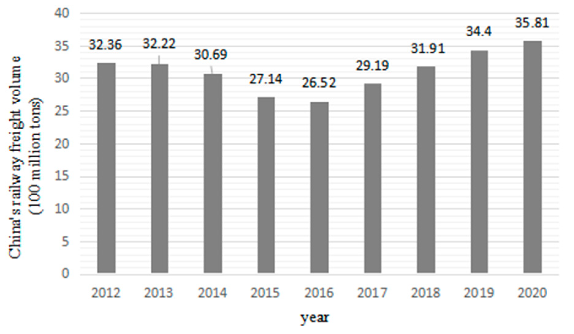
With the characteristics of high speed, large volume, low energy consumption, little pollution, safety and reliability, railway transportation has become the main transportation mode in the modern transportation system in China (see Figure 1 and Figure 2) [1,2,3] and plays an important role in the development of the national economy.
As an important national infrastructure and popular means of transportation, railway is the backbone of China’s comprehensive transportation system. With the continuous acceleration of China’s urbanization process and the urban expansion, railway construction has entered a period of rapid development, and the railway plays an increasingly important role in people’s choice of travel mode (see Figure 3) [1,4].
With regard to railway reconstruction, due to the huge investment and complex factors [5,6,7], it is necessary to compare and select various construction schemes in order to optimize the scheme with more reasonable technology and economy. Therefore, the use of scientific evaluation methods is very important. At present, the method of expert scoring and evaluation with the help of fuzzy theory has been more common, but the expert scoring is more or less subjective. This paper proposes an intelligent expert combination weighting method to optimize the scheme.
The rest of this paper is structured as follows. Section 2 introduces the related work of this study. Section 3 introduces the preparatory knowledge. Section 4 puts forward the weighted scheme of intelligent expert combination. Section 5 introduces the risk factors of the railway reconstruction project and uses the method proposed in the fourth section to optimize the railway reconstruction scheme. Finally, Section 6 summarizes the whole paper.
2. The Related Work
Fuzziness, as developed in [8], is a kind of uncertainty that often appears in human decision-making problems. Fuzzy set theory deals with uncertainties happening in daily life successfully. The membership degrees can be effectively decided by a fuzzy set. However, in real-life situations, the non-membership degrees should be considered in many cases as well. Thus, Atanassov [9] introduced the concept of an intuitionistic fuzzy (IF) set that considers both membership and non-membership degrees. IF set has been implemented in numerous areas due to its ability to handle uncertain information more effectively [10,11,12,13,14,15,16,17,18,19,20,21,22,23,24]. Tao et al. [10] provided an insight with an alternative queuing method and intuitionistic fuzzy set into dynamic group MCDM, which ranked the alternatives based on preference relation. Intuitionistic fuzzy sets based on the weighted average were adopted for aggregating individual suggestions of decision makers by Singh et al. [11]. Chaira [12] suggested a novel clustering approach for segmenting lesions/tumors in mammogram images using Atanassov’s intuitionistic fuzzy set theory. Jiang et al. [13] studied a novel three-way group investment decision model under an intuitionistic fuzzy multi-attribute group decision-making environment. Wang et al. [14] put forward a novel three-way multi-attribute decision-making model in light of a probabilistic dominance relation with intuitionistic fuzzy sets. Wan and Dong [15] developed a new intuitionistic fuzzy best-worst method for multi-criteria decision making. Kumar et al. [16] formulated an intuitionistic fuzzy set theory-based, bias-corrected intuitionistic fuzzy c-means with spatial neighborhood information method for MRI image segmentation. In addition, intuitionistic fuzzy sets are extended to various forms and applied to practical problems. Senapati and Yager [17,18,19] proposed Fermatean fuzzy sets and introduced four new weighted aggregated operators, as well as defined basic operations over the Fermatean fuzzy sets. Ashraf et al. [20] introduced a new version of the picture fuzzy set, so-called spherical fuzzy sets (SFS), and discussed some operational rules. Khan et al. [21] introduced a method to solve decision-making problems using an adjustable weighted soft discernibility matrix in a generalized picture fuzzy soft set. Riaz and Hashmi [22] introduced the novel concept of the linear Diophantine fuzzy set (LDFS) with the addition of reference parameters.
Shannon used probability theory as a mathematical tool to measure information. He defined information as something that eliminates uncertainty, thus connecting information with uncertainty. Taking entropy as a measure of the uncertainty of information state, Shannon put forward the concept of information entropy. De Luca and Termini [25] studied the measurement of fuzziness of fuzzy sets, extended probabilistic information entropy to non-probabilistic information entropy and proposed axioms that fuzzy information entropy must satisfy. Szmidt and Kacprzyk [26] extended the axioms of De Luca and Termini and extended fuzzy information entropy to IF information entropy. Some scholars have conducted in-depth research in this aspect and constructed IF entropy formulae from different angles and applied it to the fields of multi-attribute decision making and pattern recognition [27,28,29,30,31,32,33,34]. Whether these entropy formulas can reasonably measure the uncertainty of IF sets is directly related to the rationality of their application. In this paper, some entropy formulas in existing literature are classified, and their advantages and disadvantages are analyzed with data. On this basis, a new IF entropy is constructed that not only considers the deviation between membership and non-membership but also includes the hesitancy in the entropy measure. The rationality of entropy is fully explained by data analysis and comparison.
In recent years, the decision-making problem with IF information has attracted many scholars’ attention [35]. Due to the complexity and uncertainty of pragmatic problems, expert group decision-making method is commonly used in decision-making problems. Expert group decision making can fully gather the experience and knowledge of various experts, making the decision-making results more scientific and reasonable. However, in the actual evaluation, experts in group decision making are influenced by numerous factors, such as knowledge structure, understanding of scheme, interest correlation and so on. They often hold different views and attitudes. How to determine the weight of experts and effectively aggregate the decision-making information of experts with different preferences has become the focus of scholars [36,37,38,39,40,41].
In traditional group decision making, the expert weighting method usually uses the consistency ratio of the judgment matrix to construct the weight coefficient, which lacks the attention to the overall consistency of group decision-making objectives. In order to surmount the shortcomings of the traditional method, a cluster analysis method is often used to realize the expert weighting in group decision making. The basic principle of expert cluster analysis is to measure the similarity degree of expert evaluation opinions according to certain standards and cluster experts based on the similarity degree. He and Lei [36] extended fuzzy C-means clustering to IF C-means clustering and proposed a clustering algorithm based on IF sets. Zhang et al. [37] and He et al. [38] proposed the concept of IF similarity, whose value is an IF number; they also constructed the IF similarity matrix, the IF equivalent matrix and its - cut matrix and gave a clustering method based on the IF similarity matrix. Wang et al. [39] proposed a new method of an IF similar matrix, avoided the tedious process of calculating an IF equivalent matrix and used the membership degrees of elements in an IF similar matrix to cluster. Zhou et al. [40] conducted cluster analysis on experts according to the principle of entropy, used information similarity coefficients to measure the similarity degrees of expert opinions and then classified the experts.
The above clustering methods have the following problems when clustering IF information.
- (1)
- In reference [36], the clustering results of IF sets are expressed in real numbers, which does not accord with the characteristics of IF sets.
- (2)
- (3)
- Reference [39] reduced the amount of calculation, but after obtaining the IF similarity matrix, only membership degree is used for clustering, ignoring non-membership degree and hesitation degree, which will inevitably cause the loss of information.
- (4)
- In literature [40], there is no analysis on the value of the clustering threshold. The value directly affects the clustering results, so the rationality of the value is particularly important.
Considering the above situation, this paper proposes a method of clustering and weighting experts based on IF entropy. According to the evaluation information of IF numbers given by experts, a new IF similarity measure is constructed, whose value is an IF number. Then the decision matrix is transformed into a similar matrix. By analyzing the change rate of the threshold and designing the risk parameters, the decision maker can choose the appropriate clustering threshold and risk parameters so as to obtain the reasonable expert clustering results, and based on this result, experts are weighted between categories. It can make more experts in a category, so that the weight of the category is greater, which reflects the important principle of the minority obeying the majority in group decision making. Using the new IF entropy proposed in this paper, the experts in the same category with clear logic and an accurate evaluation can get a larger weight. The total weight of experts is determined by synthesizing the weight between categories and within categories. Finally, the IF weighted aggregation operator is used to aggregate weighted experts and their IF information, and the alternatives are optimized and sorted.
3. Preliminaries
In the following part, we introduce some basic concepts, which will be used in the next sections.
Definition 1
([9]). Let be a given universal set. An IF set is an object having the form where the function defines the degree of membership, and defines the degree of non-membership of the element , respectively, and for every , it holds that . Furthermore, for any IF set and , is called the hesitancy degree of . All IF sets on are denoted as .
For simplicity, Xu and Chen [41] denotedas an IF number (IFN), whereandare the degree of membership and the degree of non-membership of the elementto, respectively.
The basic operational laws of IF set defined by Atanassov [9] are introduced as follows:
Definition 2
- (1)
- if and only ifandfor all
- (2)
- if and only ifand;
- (3)
- The complementary set of, denoted by, is
- (4)
- ;
- (5)
- calledless fuzzy than, i.e., for
- if, then,;
- if, then,.
Definition 3
([9]). Let and be two IF sets and be the weight vector of the element , where and . The weighted Hamming distance for and is defined as follows:
Definition 4
- (1)
- if and only ifis a crisp set;
- (2)
- if and only if;
- (3)
- ;
- (4)
- If, then.
Definition 5
Definition 6
([37]). Let and be three IF sets. is called an IF similarity measure of and if it satisfies the following properties:
- (1)
- is an IFN;
- (2)
- if and only if;
- (3)
- =;
- (4)
- If, then, and.
Definition 7
([42]). The membership degree is expressed as , and the non-membership degree is expressed as . If an IF matrix where satisfies the following conditions:
- (1)
- Reflexivity:
- (2)
- Symmetry:
then is called an IF similarity matrix.
In order to compare the magnitudes of two IF sets, Xu and Yager [43] introduced the score and accuracy functions for IF sets and gave a simple comparison law as follows:
Definition 8
([43]). Let be an IFN; the score function and accuracy function of can be defined, respectively, as follows:
Obviously,.
Based on the score and accuracy functions, a comparison law for IF set is introduced as below:
Letandbe two IF sets,andbe the scores ofand, respectively, andandbe the accuracy degrees ofand, respectively; then,
- (1)
- If, then.
- (2)
- If, then.
The weighted aggregation operator for an IF set developed by Xu and Yager [43] is presented as follows:
Definition 9
([43]). Let be a collection of IF sets, and be the weight vector of , where indicates the importance degree of , satisfying and , and let . If
then the function is called the IF weighted aggregation operator.
4. Our Proposed Intelligent Expert Combination Weighting Scheme
4.1. A New IF Entropy
The uncertainty of IF sets is embodied in fuzziness and intuitionism. Fuzziness is determined by the difference between membership and non-membership. Intuitionism is determined by its hesitation. Therefore, entropy is used as a tool to describe the uncertainty of IF sets; the difference between membership and non-membership and their hesitation should be considered at the same time. Only in this way can the degree of uncertainty be reflected more fully. Next, we will classify the existing entropy formulas according to whether they describe the fuzziness and intuitiveness of IF sets. In addition, the motivation behind the origination of fuzzy and non-standard fuzzy models is their intimacy with human thinking. Therefore, if an entropy measure does not meet some cognitive aspect, we call it a counterintuitive case.
In this section, suppose that is an IF set.
(1) The entropy measure only describes the fuzziness of IF sets. For example, the IF entropy measure of Ye [27] is
The IF entropy measure of Zeng and Li [28] is
The IF entropy measure of Zhang and Jiang [29] is
The exponential IF entropy measure of Verma and Sharma [30] is
Example 1.
Letandbe two IF sets. Calculate the entropy ofandwith the entropy formulae,,and.
According to the above formulae, the results are as follows:
- , ,
- , .
It can be seen thatbelongs to IF setsand; the absolute value of deviation between membership and non-membership is equal; and the hesitation degree increases, so the uncertainty ofis smaller than. However, the entropy formulae,,andcalculated the entropy of two IF sets as equal. In fact, for any IF setsandiffor all, then any entropy formulaabove is adopted, and all of them have. These are counterintuitive situations.
(2) The entropy measure only describes the intuitionism of IF sets.
Example 2.
Letandbe two IF sets. Calculate the entropy ofandwith the entropy formula.
From Formula, we can get the following results:. For IF setsand, the hesitancy degree of elementis equal, but the absolute value of the deviation between the membership degree and non-membership degree ofis greater than that of, so the uncertainty ofis obviously smaller than that of. However, the entropy formulae,,andcalculated the entropy of two IF sets as equal, which is inconsistent with people’s intuition. In fact, for any IF setsand, iffor all, then any entropy formulaabove is adopted, and all of them have.
(3) The entropy measure includes both the fuzziness and intuitionism of IF sets. However, some situations cannot be well distinguished.
For example, we show the IF entropy measure of Wang and Wang [32]:
The IF entropy measure of Wei et al. [33] is the following:
Example 3.
Letandbe two IF sets. Obviously, the fuzziness ofis greater than that of. Calculate the entropies ofandwith the entropy formulaeand.
We can get the following results:
which are counterintuitive.
For example, the IF entropy measure of Liu and Ren [34] is
Example 4.
Letandbe two IF sets. Obviously, the fuzzinesses ofandare not equal. However, calculating the entropy ofandwith the entropy formulawe have.
Motivation: we can see that some existing cosine and cotangent function-based entropy measures have no ability to discriminate some IF sets, and there are counterintuitive phenomena, such as the cases of Example 1 to 4. In this paper, we are also devoted to the development of IF entropy measures. We propose a new intuitionistic fuzzy entropy based on a cotangent function, which is an improvement of Wang’s entropy [32], as follows:
which not only considers the deviation between membership and non-membership degrees , but also considers the hesitancy degree of the IF set.
Theorem 1.
The measure given by Equation (3) is an IF entropy.
Proof.
To prove the measure given by Equation (3) is an IF entropy, we only need to prove it satisfies the properties in Definition 4. Obviously, for every , we have:
then
Thus, we have .
(i) Let be a crisp set, i.e., for , we have or . It is obvious that .
If , i.e., , then , we have .
Thus , amd then we have or . Therefore, is a crisp set.
(ii) Let ,; according to Equation (3), we have .
Now we assume that ; then for all , we have: , then , and we can obtain the conclusion for all .
(iii) By and Equation (3), we have:
(iv) Construct the function:
Now, when , we have ; we need to prove that the function is increasing with and decreasing with .
We can easily derive the partial derivatives of to and to , respectively:
When , we have ; then, is increasing with and decreasing with ; thus, when and are satisfied, we have .
So that is, holds.
Similarly, we can prove that when , , then is decreasing with and increasing with , thus when and is satisfied, so we have .
Therefore, if , we have , i.e., . □
From Equation (3), the entropies of in Examples 1 to 4 can be obtained as follows:
The calculation results are in agreement with our intuition.
According to the above examples, we see that the proposed entropy measure has a better performance than the entropy measures . Furthermore, the new entropy measure considers the two aspects of the IF set (i.e., the uncertainty depicted by the derivation of membership and non-membership and the hesitancy degree reflected by the hesitation degree of the IF set), and thus the proposed entropy measure is a good entropy measure formula of the IF set.
4.2. Clustering Method of Group Decision Experts
For group decision-making problems, suppose that is a set of schemes, and is a set of decision makers. The evaluation values decision makers to schemes are expressed by IF number , where and are the membership (satisfaction) and non-membership (dissatisfaction) degrees of the decision maker to the scheme with respect to the fuzzy concept so that they satisfy the conditions and (; ).
Thus, a group decision-making problem can be expressed by the decision matrix as follows:
4.2.1. A New IF Similarity Measure
To measure the similarities among any form of data is an important topic [44,45]. The measures used to find the resemblance between data is called a similarity measure. It has different applications in classification, medical diagnosis, pattern recognition, data mining, clustering [46], decision making and image processing. Khan et al. [47] proposed a newly similarity measure for a q-rung orthopair fuzzy set based on a cosine and cotangent function. Chen and Chang [48] proposed a new similarity measure between Atanassov’s intuitionistic fuzzy sets (AIFSs) based on transformation techniques and applied the proposed similarity measure between AIFSs to deal with pattern recognition problems. Beliakov et al. [49] presented a new approach for defining similarity measures for AIFSs and applied it to image segmentation. Lohani et al. [50] presented a novel probabilistic similarity measure (PSM) for AIFSs and developed the novel probabilistic λ-cutting algorithm for clustering. Liu et al. [51] proposed a new intuitionistic fuzzy similarity measure, introduced it into intuitionistic fuzzy decision system and proposed an intuitionistic fuzzy three branch decision method based on intuitionistic fuzzy similarity. Mei [52] constructed a similarity model between intuitionistic fuzzy sets and applied it to dynamic intuitionistic fuzzy multi-attribute decision making.
At present, most of the existing similarity measures are expressed in real numbers, which is not in line with the characteristics of intuitionistic fuzzy sets. In this section, we define a new IF similarity measure whose value is an IF number.
For any two experts and , let
where is the weight of scheme for all and and is a parameter.
Let
Theorem 2.
Letandbe two IF sets; then,
is the IF similarity measure ofand.
Proof.
To prove the measure given by Equation (4) is an IF similarity measure of and , we only need to prove that it satisfies the properties in Definition 6.
First, we prove that is the form of an IFN.
Because and , so , and . This proves that is the form of an IFN.
Let ; we have
And , so . Because of the arbitrariness of , we get and for all , that is, .
Now we assume that ; then for all , we have ; we can obtain and ,, that is, .
Property 3 clearly holds.
If , i.e., for all ,then for all .
We have and ; therefore,, and , that is,. Similarly, it can be proved that .
This theorem is proved. □
For IF similarity measure Equation (4), since each scheme is equal, this paper takes for all . Using this formula, the IF decision matrix can be transformed into the IF similar matrix , where is an IFN.
The IF decision matrix can be transformed into the IF similarity matrix by using the IF similarity formula proposed in this paper, where is an IFN.
People’s pursuit of risk varies from person to person. Let be the risk factor; then the IF similarity matrix can be transformed into a real matrix where .
4.2.2. Threshold Change Rate Analysis Method
The method of Zhou et al. [40] is adopted in this section.
Let the clustering threshold , where . If
then elements and are considered to have the same properties. The closer the threshold is to 1, the finer the classification is.
In Zhou et al. [40], the selection of the optimal clustering threshold can be deter-mined by analyzing the change rate of . The rate of change is given as follows:
where is the clustering times of from large to small, and are the number of objects in the -th and -th clustering, respectively, and and are the thresholds for the -th and -th clustering, respectively. If
then the threshold value of clustering is the best.
It can be seen from Equation (5) that the greater the change rate of the clustering threshold is, the greater the difference between the corresponding two clusters and the more obvious the boundary between classes. When is the maximum value, its corresponding is the optimal clustering threshold value, which can make the difference between the clusters obtained by the -th clustering to be the largest, thus realizing the purpose and significance of classification.
4.3. Analysis of Group Decision Making Expert Group Weighting
In group decision-making problems, because each expert has a different specialty, experience and preference, their evaluation information should be treated differently. In order to reflect the status and importance of each expert in decision making, it is of great significance to determine the expert weight reasonably.
Two aspects need to be considered in expert weight, namely, the weight between categories and the weight within categories. The weight between categories mainly considers the number of experts in the category of experts. For the category with large capacity, the evaluation results given by experts represent the opinions of most experts, so the corresponding categories should be given a larger weight, which reflects the principle that the minority is subordinate to the majority, while the category with smaller capacity should be given a smaller weight.
Suppose that experts are divided into categories; the number of experts in the category is ; and the weights between the expert categories are as follows:
The weight of experts within the category can be measured by the information contained in an IF evaluation value given by experts. Entropy is a measure of information uncertainty and information quantity. If the entropy of the evaluation information given by an expert is smaller, the uncertainty of the evaluation information is smaller, which means that the logic of the expert is clearer; the amount of information provided is greater; and the role of the expert in the comprehensive evaluation is greater, so the expert should be given more weight. Therefore, the weight of experts within the category can be measured by IF entropy.
The evaluation vector of expert is
The IF entropy corresponding to Equation (1) is expressed as follows:
The internal weight of the expert in category is as follows:
By linear weighting and , the total weight of experts is obtained:
4.4. Intelligent Expert Combination Weighting Algorithm
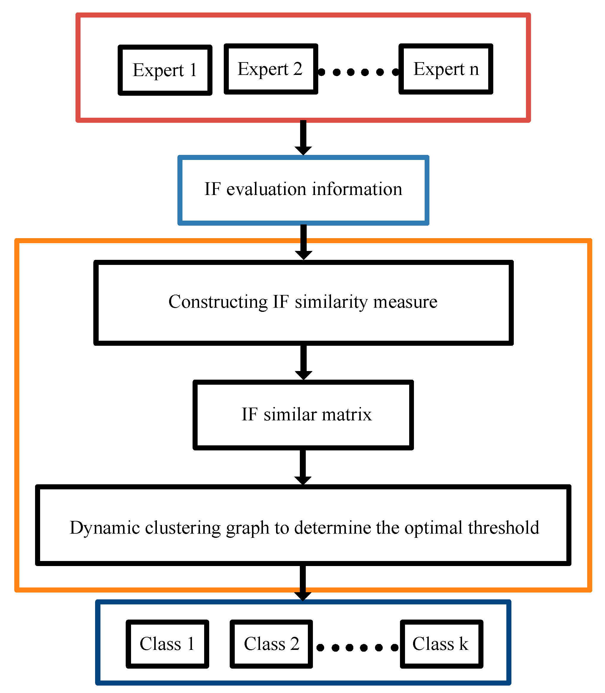
A cluster analysis method is often used to realize the expert weighting in group decision making. The basic principle of expert cluster analysis is to measure the similarity degree of expert evaluation opinions according to certain standards and cluster experts based on the similarity degree. In short, Figure 4 shows the general scheme of the expert clustering method.
To sum up, this paper proposes an expert combination weighting scheme for group decision making, and obtains the following algorithm, which we call the intelligent expert combination weighting algorithm (see Algorithm 1).
| Algorithm 1. Intelligent expert combination weighting algorithm |
| Input the IF decision matrix given by experts where |
| 1: For implement. |
| 2: For implement. |
| 3: For implement. |
| 4: The IF similarity measure between experts is calculated according to formula (4). |
| 5: End for |
| 6: Let |
| 7: End for |
| 8: End for |
| 9: The IF decision matrix is transformed into the similarity matrix |
| 10: By selecting the risk factor β, the IF similarity matrix is transformed into the real matrix |
| 11: According to the real matrix , the dynamic clustering graph is drawn, and the optimal clustering threshold is determined by Formulae (6) and (7). According to this threshold, experts are classified into L categories. |
| 12: For implement. |
| 13: Using Formula (8), the weight of experts between categories λl is determined. |
| 14: For implement. |
| 15: Using Formula (8), the weight of experts between categories alk is determined. |
| 16: Formula (11) is used to determine the total weight of experts. ωk is calculated. |
| 17: End for. |
| 18: End for. |
| 19: For implement. |
| 20: For implement. |
| 21: The weighted operator (2) of IF sets is used to aggregate expert IF group decision-making information. |
| 22: End for. |
| 23: According to definition 8, the scores and accuracy values of each scheme xi are obtained. |
| 24: End for. |
| 25: return The results of the ranking of schemes xi. |
5. Performance Analysis
The railway is an important national infrastructure and livelihood project. It is a resource-saving and environment-friendly mode of transportation. In recent years, China’s railway development has made remarkable achievements, but compared with the needs of economic and social development, other modes of transportation and advanced foreign railway technique, the railway in China is still a weak part of the whole transportation system [53,54]. In order to further accelerate railway construction, expand the scale of railway network and improve the layout structure and quality, the state promulgated the medium and long term railway network plan, which puts forward a series of railway plans, including the plan for railway reconstruction.
The railway reconstruction project is carried out under a series of communication, coordination and cooperation efforts, and the complex work is arranged in a limited work area, so it has encountered many unexpected challenges, such as carelessness or inadequate planning, which may lead to accidents and cause significant damage to life, assets, environment and society. According to literature [55], we can conclude that there are about seven types of risks in railway reconstruction projects, including financial and economic risks, contract and legal risks, subcontractor related risks, operation and safety risks, political and social risks, design risks and force majeure risks.
It is assumed that nine experts form a decision-making group to rank five alternatives from the seven evaluation attributes above. Evaluation alternatives always contain ambiguity and diversity of meaning. In addition, in terms of qualitative attributes, human assessment is subjective and therefore inaccurate. In this case, an IF set is very advantageous; it can describe the decision process more accurately. IF sets are used in this study. After expert investigation and statistical analysis, we can get the satisfaction degree and dissatisfaction given by each expert for each scheme . The specific data are given in Table 1.
The calculation steps of the proposed method are given as follows:
Step 1. According to Equation (4), the IF similarity matrix is obtained as follows:
Step 2. By selecting the risk factor , i.e., moderate risk, the real matrix is obtained.
Step 3. According to Equation (5), let take all the values in turn to get a series of classifications, and then draw a dynamic clustering graph according to Equations (5) and (6), as shown in Figure 5.
According to Equation (6), we have
Since it is meaningless for each expert to become a category or all experts to be classified into one category, we do not consider ; then, we have .
Therefore, taking as the optimal clustering threshold, the clustering result is the most reasonable and consistent with the actual situation, and the clustering results are shown in Figure 6. We can see that the corresponding clustering results are as follows:
{(1 4 8), (3 5 7), (2 9), (6)}
Step 4. According to Equation (8), the weight of experts between categories is as follows:
Step 5. According to Equation (9), the entropy vector of the expert group is obtained as follows:
(0.6868, 0.7405, 0.5538, 0.7364, 0.4995, 0.5935, 0.5507, 0.7159, 0.7339)
According to Equation (10), the weight of experts within the category is shown in Table 2.
Step 6. We weight and linearly to get the total weight vector of experts as follows:
(0.1424, 0.0859, 0.1251, 0.1198, 0.1403, 0.0435, 0.1260, 0.1291, 0.0748).
Step 7. According to the total weight of nine experts, the weighted aggregation operator given by Equation (2) is used to aggregate the expert information, and the comprehensive evaluation vector is obtained as follows:
(0.3616, 0.4504), (0.5226, 0.3878), (0.5932, 0.3218), (0.4749, 0.3853), (0.4972, 0.3718).
According to Equation (1), the scores and accuracy values of the comprehensive evaluation vector are calculated as follows:
Therefore, the priority of the five alternatives is , and the optimal one is .
6. Conclusions and Future Work
This article listed some counterintuitive phenomena of some existing intuitionistic fuzzy entropies. We defined an improved intuitionistic fuzzy entropy based on a cotangent function and a new IF similarity measure whose value is an IF number, applied them to the expert weight problem of group decision making and put forward the expert weight combination weighting scheme. Finally, this method was applied to a railway reconstruction case to illustrate the effectiveness of the method.
In the future, we will apply the expert weight combination weighting scheme proposed in this paper to situations in real life. We will also formulate this kind of entropy measure and similarity measures for an interval-valued IF set [56], Fermat fuzzy set, spherical fuzzy set, t-spherical fuzzy set, picture fuzzy set, single valued neutrosophic set [55,57], Plithogenic set [58] and linear fuzzy set.
While studying the theoretical method, this paper used numerical examples rather than the actual production data, which is the limitation of this paper. In the future research, we will apply the expert weight combination weighting scheme proposed in this paper to practical production problems.
Author Contributions
L.Z. and H.R. designed the method and wrote the paper; T.Y. and N.X. analyzed the data. All authors have read and agreed to the published version of the manuscript.
Funding
This work was mainly supported by the National Natural Science Foundation of China (No. 71661012) and scientific research project of the Jiangxi Provincial Department of Education (No. GJJ210827).
Institutional Review Board Statement
Not applicable.
Informed Consent Statement
Not applicable.
Data Availability Statement
The data used to support the findings of this study are included within the article.
Conflicts of Interest
The authors declared that they have no conflict of interest to this work.
References
- Xie, Y.; Kou, Y.; Jiang, M.; Yu, W. Development and technical prospect of China railway. High Speed Railway Technol. 2020, 11, 11–16. [Google Scholar]
- Li, Y.B. Research on the current situation and development direction of railway freight transportation in China. Intell. City 2019, 5, 133–134. [Google Scholar]
- Fu, Z.; Zhong, M.; Li, Z. Development and innovation of Chinese railways over past century. Chin. Rail. 2021, 7, 1–7. [Google Scholar]
- Li, Z.; Xie, R.; Sun, L.; Huang, T. A survey of mobile edge computing Telecommunications Science. Chin. Rail. 2014, 2, 9–13. [Google Scholar]
- Lu, S.-T.; Yu, S.-H.; Chang, D.-S. Using fuzzy multiple criteria decision-making approach for assessing the risk of railway reconstruction project in Taiwan. Sci. Word J. 2014, 2014, 239793. [Google Scholar] [CrossRef] [Green Version]
- Wang, M.; Xie, H. Present situation analysis and discussion on development of Chinese railway construction market. J. Rail. Sci. Eng. 2008, 5, 63–67. [Google Scholar]
- Zhang, Z. Analysis on risks in construction of railway engineering projects and exploration for their prevention. Rail. Stan. Desi. 2010, 9, 51–52. [Google Scholar]
- Zadeh, L. Fuzzy sets. Inf. Control 1965, 8, 338–353. [Google Scholar] [CrossRef] [Green Version]
- Atanassov, K. Intuitionistic fuzzy sets. Fuzzy Sets Syst. 1986, 20, 87–96. [Google Scholar] [CrossRef]
- Tao, P.; Liu, Z.; Cai, R.; Kang, H. A dynamic group MCDM model with intuitionistic fuzzy set: Perspective of alternative queuing method. Inf. Sci. 2021, 555, 85–103. [Google Scholar] [CrossRef]
- Singh, M.; Rathi, R.; Antony, J.; Garza-Reyes, J. Lean six sigma project selection in a manufacturing environment using hybrid methodology based on intuitionistic fuzzy MADM approach. IEEE Trans. Eng. Manag. 2021, 99, 1–15. [Google Scholar] [CrossRef]
- Chaira, T. An intuitionistic fuzzy clustering approach for detection of abnormal regions in mammogram images. J. Digit. Imaging 2021, 34, 428–439. [Google Scholar] [CrossRef] [PubMed]
- Jiang, H.B.; Hu, B.Q. A novel three-way group investment decision model under intuitionistic fuzzy multi-attribute group decision-making environment. Inf. Sci. 2021, 569, 557–581. [Google Scholar] [CrossRef]
- Wang, W.; Zhan, J.; Mi, J. A three-way decision approach with probabilistic dominance relations under intuitionistic fuzzy information. Inf. Sci. 2022, 582, 114–145. [Google Scholar] [CrossRef]
- Wan, S.; Dong, J. A novel extension of best-worst method with intuitionistic fuzzy reference comparisons. IEEE Trans. Fuzzy Syst. 2021, 99, 1. [Google Scholar] [CrossRef]
- Kumar, D.; Agrawal, R.; Kumar, P. Bias-corrected intuitionistic fuzzy c-means with spatial neighborhood information ap proach for human brain MRI image segmentation. IEEE Trans. Fuzzy Syst. 2020. [Google Scholar] [CrossRef]
- Senapati, T.; Yager, R. Fermatean fuzzy sets. J. Ambient Intell. Humaniz. Comput. 2020, 11, 663–674. [Google Scholar] [CrossRef]
- Senapati, T.; Yager, R. Fermatean fuzzy weighted averaging/geometric operators and its application in multi-criteria decision-making methods—Science Direct. Eng. Appl. Artif. Intell. 2019, 85, 112–121. [Google Scholar] [CrossRef]
- Senapati, T.; Yager, R. Some new operations over fermatean fuzzy numbers and application of fermatean fuzzy WPM in multiple criteria decision making. Informatica 2019, 2, 391–412. [Google Scholar] [CrossRef] [Green Version]
- Ashraf, S.; Abdullah, S.; Mahmood, T.; Ghani, F. Spherical fuzzy sets and their applications in multi-attribute decision making problems. J. Intell. Fuzzy Syst. 2019, 36, 2829–2844. [Google Scholar] [CrossRef]
- Khan, M.; Kumam, P.; Liu, P.; Kumam, W.; Rehman, H. An adjustable weighted soft discernibility matrix based on generalized picture fuzzy soft set and its applications in decision making. J. Intell. Fuzzy Syst. 2020, 38, 2103–2118. [Google Scholar] [CrossRef]
- Riaz, M.; Hashmi, M. Linear Diophantine fuzzy set and its applications towards multi-attribute decision-making problems. J. Intell. Fuzzy Syst. 2019, 37, 5417–5439. [Google Scholar] [CrossRef]
- Gao, K.; Han, F.; Dong, P.; Xiong, N.; Du, R. Connected vehicle as a mobile sensor for real time queue length at signalized intersections. Sensors 2019, 19, 2059. [Google Scholar] [CrossRef] [PubMed] [Green Version]
- Zhang, Q.; Zhou, C.; Tian, Y.; Xiong, N.; Qin, Y.; Hu, B. A fuzzy probability Bayesian network approach for dynamic cybersecurity risk assessment in industrial control systems. IEEE Trans. Ind. Inform. 2017, 14, 2497–2506. [Google Scholar] [CrossRef] [Green Version]
- Luca, A.; Termini, S. A definition of a nonprobabilistie entropy in the setting of fuzzy sets theory. Inf. Control 1972, 3, 301–312. [Google Scholar] [CrossRef] [Green Version]
- Szmidt, E.; Kacprzyk, J. Entropy for intuitionistic fuzzy sets. Fuzzy Sets Syst. 2001, 118, 467–477. [Google Scholar] [CrossRef]
- Ye, J. Two effective measures of intuitionistic fuzzy entropy. Computing 2010, 87, 55–62. [Google Scholar] [CrossRef]
- Zeng, W.; Li, H. Relationship between similarity measure and entropy of interval valued fuzzy sets. Fuzzy Sets Syst. 2006, 157, 1477–1484. [Google Scholar] [CrossRef]
- Zhang, Q.; Jiang, S. A note on information entropy measures for vague sets and its applications. Inf. Sci. 2008, 178, 4184–4191. [Google Scholar] [CrossRef]
- Verma, R.; Sharma, B. Exponential entropy on intuitionistic fuzzy sets. Kybernetika 2013, 49, 114–127. [Google Scholar]
- Burillo, P.; Bustince, H. Entropy on intuitionistic fuzzy sets and on interval-valued fuzzy sets. Fuzzy Sets Syst. 1996, 78, 305–316. [Google Scholar] [CrossRef]
- Wang, J.; Wang, P. Intuitionistic linguistic fuzzy multi-criteria decision-making method based on intuitionistic fuzzy entropy. Control Decis. 2012, 27, 1694–1698. [Google Scholar]
- Wei, C.; Gao, Z.; Guo, T. An intuitionistic fuzzy entropy measure based on trigonometric function. Control Decis. 2012, 27, 571–574. [Google Scholar]
- Liu, M.; Ren, H. A new intuitionistic fuzzy entropy and application in multi-attribute decision making. Informatica 2014, 5, 587–601. [Google Scholar] [CrossRef] [Green Version]
- Ai, C.; Feng, F.; Li, J.; Liu, K. AHP method of subjective group decision-making based on interval number judgment matrix and fuzzy clustering analysis. Control Decis. 2019, 35, 41–45. [Google Scholar]
- He, Z.; Lei, Y. Research on intuitionistic fuzzy C-means clustering algorithm. Control Decis. 2011, 26, 847–850. [Google Scholar]
- Zhang, H.; Xu, Z.; Chen, Q. On clustering approach to intuitionistic fuzzy sets. Control Decis. 2007, 22, 882–888. [Google Scholar]
- He, Z.; Lei, Y.; Wang, G. Target recognition based on intuitionistic fuzzy clustering. J. Syst. Eng. Electron. 2011, 6, 1283–1286. [Google Scholar]
- Wang, Z.; Xu, Z.; Liu, S.; Tang, J. A netting clustering analysis method under intuitionistic fuzzy environment. Appl. Soft Comput. 2011, 11, 5558–5564. [Google Scholar] [CrossRef]
- Zhuo, X.; Zhang, F.; Hui, X.; Li, K. Method for determining experts’ weights based on entropy and cluster analysis. Control Decis. 2011, 26, 153–156. [Google Scholar]
- Xu, Z.; Chen, J. An overview of distance and similarity measures of intuitionistic fuzzy sets. Int. J. Uncertain. Fuzz. 2008, 16, 529–555. [Google Scholar] [CrossRef]
- Zhang, Z.; Chen, S.; Wang, C. Group decision making with incomplete intuitionistic multiplicative preference relations. Inf. Sci. 2020, 516, 560–571. [Google Scholar] [CrossRef]
- Xu, Z.S.; Yager, R.R. Some geometric aggregation operators based on intuitionistic fuzzy sets. Int. J. Gen. Syst. 2006, 35, 417–433. [Google Scholar] [CrossRef]
- Huang, S.; Liu, A.; Zhang, S.; Wang, T.; Xiong, N. BD-VTE: A novel baseline data based verifiable trust evaluation scheme for smart network systems. IEEE Trans. Netw. Sci. Eng. 2020, 8, 2087–2105. [Google Scholar] [CrossRef]
- Wu, M.; Tan, L.; Xiong, N. A structure fidelity approach for big data collection in wireless sensor networks. Sensors 2015, 15, 248–273. [Google Scholar] [CrossRef] [Green Version]
- Li, H.; Liu, J.; Wu, K.; Yang, Z.; Liu, R.; Xiong, N. Spatio-temporal vessel trajectory clustering based on data mapping and density. IEEE Access 2018, 6, 58939–58954. [Google Scholar] [CrossRef]
- Khan, M.; Kumam, P.; Alreshidi, N.; Kumam, W. Improved cosine and cotangent function-based similarity measures for q-rung orthopair fuzzy sets and TOPSIS method. Complex Intell. Syst. 2021, 7, 2679–2696. [Google Scholar] [CrossRef]
- Chen, S.; Chang, C. A novel similarity measure between Atanassov’s intuitionistic fuzzy sets based on transformation techniques with applications to pattern recognition. Inf. Sci. 2015, 291, 96–114. [Google Scholar] [CrossRef]
- Beliakov, G.; Pagola, M.; Wilkin, T. Vector valued similarity measures for Atanassov’s intuitionistic fuzzy sets. Inf. Sci. 2014, 280, 352–367. [Google Scholar] [CrossRef]
- Lohani, Q.; Solanki, R.; Muhuri, P. Novel adaptive clustering algorithms based on a probabilistic similarity measure over Atanassov intuitionistic fuzzy set. IEEE Trans. Fuzzy Syst. 2018, 6, 3715–3729. [Google Scholar] [CrossRef]
- Liu, J.; Zhou, X.; Li, H.; Huang, B.; Gu, P. An intuitionistic fuzzy three-way decision method based on intuitionistic fuzzy similarity degrees. Syst. Eng. Theory Pract. 2019, 39, 1550–1564. [Google Scholar]
- Mei, X. Dynamic intuitionistic fuzzy multi-attribute decision making method based on similarity. Stat. Decis. 2016, 15, 22–24. [Google Scholar]
- Tang, Y. Comparison and analysis of domestic and foreign railway energy consumption. Rail. Tran. Econ. 2018, 40, 97–103. [Google Scholar]
- Gao, F. A study on the current situation and development strategies of China’s railway restructuring. Railw. Freight Transport. 2020, 38, 15–19. [Google Scholar]
- Chai, J.S.; Selvachandran, G.; Smarandache, F.; Gerogiannis, V.C.; Son, L.H.; Bui, Q.-T.; Vo, B. New similarity measures for single-valued neutrosophic sets with applications in pattern recognition and medical diagnosis problems. Complex Intell. Syst. 2021, 7, 703–723. [Google Scholar] [CrossRef]
- Garg, H. Generalized intuitionistic fuzzy entropy-based approach for solving multi-attribute decision-making problems with unknown attribute weights. Proc. Natl. Acad. Sci. USA 2017, 89, 129–139. [Google Scholar] [CrossRef]
- Majumdar, P. On new measures of uncertainty for neutrosophic sets. Neutrosophic Sets Syst. 2017, 17, 50–57. [Google Scholar]
- Quek, S.G.; Selvachandran, G.; Smarandache, F.; Vimala, J.; Le, S.H.; Bui, Q.-T.; Gerogiannis, V.C. Entropy measures for Plithogenic sets and applications in multi-attribute decision making. Mathematics 2020, 8, 965. [Google Scholar] [CrossRef]
Figure 1.
Business mileage of China’s railways.

Figure 2.
Total railway freight volume in China.

Figure 3.
China railway passenger volume.

Figure 4.
The general scheme of expert clustering method.

Figure 5.
Dynamic clustering graph.

Figure 6.
Clustering results.


Table 1.
Expert evaluation information on the program.
| Expert | |||||
|---|---|---|---|---|---|
| <0.43,0.45> | <0.24,0.70> | <0.57,0.40> | <0.29,0.55> | <0.25,0.60> | |
| <0.58,0.30> | <0.37,0.52> | <0.30,0.50> | <0.55,0.35> | <0.35,0.50> | |
| <0.31,0.61> | <0.74,0.22> | <0.70,0.25> | <0.50,0.40> | <0.70,0.20> | |
| <0.44,0.45> | <0.31,0.60> | <0.56,0.40> | <0.31,0.52> | <0.24,0.60> | |
| <0.31,0.60> | <0.70,0.20> | <0.75,0.20> | <0.60,0.30> | <0.68,0.20> | |
| <0.70,0.20> | <0.58,0.32> | <0.52,0.40> | <0.20,0.70> | <0.60,0.30> | |
| <0.38,0.52> | <0.72,0.21> | <0.68,0.22> | <0.61,0.30> | <0.70,0.22> | |
| <0.41,0.40> | <0.28,0.60> | <0.55,0.35> | <0.30,0.55> | <0.26,0.60> | |
| <0.56,0.34> | <0.40,0.50> | <0.30,0.40> | <0.71,0.10> | <0.38,0.45> |
Table 2.
The weight of experts within the category.
| Category | The Weight of Experts within the Category |
| Category 1 | |
| Category 2 | |
| Category 3 | |
| Category 4 |
Publisher’s Note: MDPI stays neutral with regard to jurisdictional claims in published maps and institutional affiliations. |
© 2022 by the authors. Licensee MDPI, Basel, Switzerland. This article is an open access article distributed under the terms and conditions of the Creative Commons Attribution (CC BY) license (https://creativecommons.org/licenses/by/4.0/).
Share and Cite
MDPI and ACS Style
Zeng, L.; Ren, H.; Yang, T.; Xiong, N. An Intelligent Expert Combination Weighting Scheme for Group Decision Making in Railway Reconstruction. Mathematics 2022, 10, 549. https://0-doi-org.brum.beds.ac.uk/10.3390/math10040549
AMA Style
Zeng L, Ren H, Yang T, Xiong N. An Intelligent Expert Combination Weighting Scheme for Group Decision Making in Railway Reconstruction. Mathematics. 2022; 10(4):549. https://0-doi-org.brum.beds.ac.uk/10.3390/math10040549
Chicago/Turabian StyleZeng, Lihua, Haiping Ren, Tonghua Yang, and Neal Xiong. 2022. "An Intelligent Expert Combination Weighting Scheme for Group Decision Making in Railway Reconstruction" Mathematics 10, no. 4: 549. https://0-doi-org.brum.beds.ac.uk/10.3390/math10040549
Note that from the first issue of 2016, this journal uses article numbers instead of page numbers. See further details here.