Empirical Study of Data-Driven Evolutionary Algorithms in Noisy Environments

Abstract

For computationally intensive problems, data-driven evolutionary algorithms (DDEAs) are advantageous for low computational budgets because they build surrogate models based on historical data to approximate the expensive evaluation. Real-world optimization problems are highly susceptible to noisy data, but most of the existing DDEAs are developed and tested on ideal and clean environments; hence, their performance is uncertain in practice. In order to discover how DDEAs are affected by noisy data, this paper empirically studied the performance of DDEAs in different noisy environments. To fulfill the research purpose, we implemented four representative DDEAs and tested them on common benchmark problems with noise simulations in a systematic manner. Specifically, the simulation of noisy environments considered different levels of noise intensity and probability. The experimental analysis revealed the association relationships among noisy environments, benchmark problems and the performance of DDEAs. The analysis showed that noise will generally cause deterioration of the DDEA’s performance in most cases, but the effects could vary with different types of problem landscapes and different designs of DDEAs.

1. Introduction

Data-driven evolutionary algorithms (DDEAs) are a superposition of evolutionary computation, machine learning and data science [1]. With the help of available data, DDEAs construct surrogate models to predict the fitness values of candidate solutions without expensive fitness evaluations. A considerable amount of literature has been published on DDEAs owing to their effectiveness for solving real-world problems [2]. Various DDEAs have been introduced to tackle the problems of expensive fitness evaluations. However, noisy data have brought challenges to the real-world optimization of DDEAs because the performance of DDEAs is greatly affected by noisy data [3,4]. To address this issue, there is an urgent need to investigate the degree to which DDEAs are affected by different noisy environments and the reasons for this.

DDEAs can generally be divided into online and offline DDEAs according to whether new data can be generated during the optimization process [5]. Both online and offline DDEAs are exposed to the challenges of low quality data. The available data might be incomplete [6], imbalanced [7,8,9] and noisy in quite common cases [10]. In this work, we focused on noisy data-driven optimization problems. Apparently, the quality of surrogate models would decline if they were trained on noisy datasets instead of the ideal clean datasets used in previous studies. Subsequently, the increased approximation error of solution evaluation would decrease the search efficacy of the EA population. Although this conclusion might be obvious, we have no explicit knowledge on under which circumstances and/or the degree to which noisy data affect the performance of DDEAs yet. In the literature, there are plenty of research efforts paid to analyze the traditional real evaluation-based evolutionary algorithms (denoted as REEAs in this paper) in noisy environments empirically [11,12] or theoretically [13,14,15]. However, because of the difference between REEAs and DDEAs, those observations/conclusions cannot be directly transferred from REEAs to DDEAs.

As DDEAs show their superiority to REEAs when encountering real-world problems with expensive or implicit fitness evaluations, this paper is dedicated to our performance of extensive experiments to investigate the performance of DDEAs in noisy environments. Inspired by the progress in simulating noisy environments [16,17,18], we proposed to add noise to the test environments of DDEAs by making the following assumption: the exact fitness value $f\left(x\right)$ can only be obtained in a certain probability $P_n$, whereas in the other cases, the obtained evaluation value is $f\left(x\right)+ϵ$, which contains a noise component. Meanwhile, the magnitude of the noisy term ϵ determines the noise intensity, which has different levels according to a signal-to-noise ratio (SNR) parameter. In addition to the simulation of the noisy environment, there remained two issues for carrying out the empirical analysis. The first issue surrounded which algorithms to test, and the second involved the selection of benchmark problems. After carefully surveying the well-known and state-of-the-art DDEA variants, we chose four representative algorithms with different characteristics: an offline data-driven evolutionary algorithm assisted by selective ensembles (DDEA-SE) [19], a social learning particle swarm optimization algorithm assisted by a multi-objective infill criterion-driven Gaussian process (MGP-SLPSO) [20], a surrogate-assisted particle swarm algorithm with the help of committee-based active learning (CAL-SAPSO) [21] and a Gaussian process-assisted evolutionary algorithm (GPEME) [22]. The above one offline DDEA and three online DDEAs are discussed in Section 2.1, Section 2.2, Section 2.3 and Section 2.4 in detail. On the other hand, five benchmark problems, which are frequently adopted for testing the performance of DDEAs [19,20,23], are chosen for testing.

Therefore, in this paper, experiments are carried out to test the four representative DDEAs on the five benchmark problems in noisy environments within different noisy levels. Our major findings are threefold. (1) The performance of DDEAs is not very altered if the noise level is low, but with increases in the noise level, the performance of DDEAs declines seriously. (2) For different benchmark problems, the noise has different effects. For example, if the problem contains rugged prominent optimum regions, the addition of noise reduces the search efficiency of the algorithms significantly. Differently, the problems in which the neighborhoods of the optima are relatively flat have a larger level of resistance to the noise, and, sometimes, they may even receive benefits from the noise. (3) Concerning different DDEAs tested in this study, the offline DDEA has advantages over the online DDEAs in noisy data-driven optimization problems.

The remainder of this paper is as follows: Section 2 introduces the main concepts of DDEAs and a brief introduction of the four DDEAs related to the experiment. In Section 3, the simulation of the noisy environment is fully explained, including the basic definitions, the noise parameter settings, and the benchmark problems. The experimental processing and analysis are detailed in Section 4, which discusses the performance of DDEAs in the noisy environment from three perspectives. Section 5 summarizes the influence of noisy environments on DDEAs and finally proposes promising future directions of DDEAs in noisy environments.

2. Data-Driven Evolutionary Algorithms (DDEAs)

The obstacle faced by traditional EAs to solving real-world optimization problems is in the need for a large number of iterations to search in the problem space. During the search process, traditional REEAs need to evaluate the fitness value of generated candidate solutions by the real evaluation model. However, in many realistic optimization problems, the evaluation of the fitness value can be expensive or time-consuming [24], which limits the search ability of traditional REEAs. To solve this problem, DDEAs are equipped with surrogate models built from evaluated data to replace part or all of the evaluations during the search. In addition to mitigating the expensive optimization problems, surrogate models can be helpful for dynamic optimization problems, such as the robust optimization-over-time method [25]. The main idea of surrogate models is to simulate the relationship between decision variables and objective variables based on historical data. Using historical data, some common surrogate models such as Kriging model [26,27], artificial neural network [28,29,30], radial basis function network [31,32,33] and other machine learning models can be trained by the corresponding training method and used for predicting the fitness value of the candidate solutions.

In order to predict the fitness value of the candidate solutions generated during the optimization, DDEAs use historical data to construct surrogate models and fit the mapping relationship between the solution space and the fitness value space. The algorithm framework of DDEAs is similar to that of traditional EAs. At the beginning, the parent population is initialized randomly. Afterwards, in each iteration of DDEAs, a series of evolutionary operations, such as crossover and mutation, are performed on parent individuals to generate offspring. To evaluate the fitness of the offspring individuals, DDEAs use the surrogate model to approximate the real value. According to the predicted fitness value of the current parent and offspring individuals, the parent individuals of the next generation are selected.

DDEAs are divided into two major types, online DDEAs and offline DDEAs, according to whether the certain number of expensive real fitness functions are allowed to be used during the optimization process [5]. Online DDEAs allow for the expensive and accurate evaluation of true fitness values. However, the number of expensive fitness evaluations is limited; thus, online DDEAs need a selection step to choose the promising candidate solutions for the expensive real fitness evaluation. Offline DDEAs can only evaluate the fitness of the candidate solutions according to the surrogate model constructed from the historical data. Because offline DDEAs are not allowed to use the real fitness function during the optimization process, more attention should be placed on the performance of the surrogate model. According to [1], we carefully selected four typical DDEAs for our research. The four algorithms mentioned below cannot represent the best algorithms among the current DDEAs, but they have different characteristics. We chose these four algorithms to investigate the performance of DDEAs in noisy environments and the influence of noisy environments on these algorithms.

2.1. DDEA-SE

DDEA-SE [34,35], by combining methods of bagging and model selection strategies, is a representative offline data-driven EA with excellent efficiency. Since no new data are available to update the model during optimization, DDEA-SE builds large numbers of surrogates based on data resampled from historical data by bagging and then adaptively selects some of the surrogates to form the ensemble learner. More specifically, DDEA-SE uses radial basis function networks as the surrogate model. Before the optimization, DDEA-SE trains $T$ surrogate models based on the historical data. In each iteration, the best individual estimated by all the base models is used to sort the base models. The sorted base models are divided into $Q$ groups, and then one model from each group is selected randomly to ensemble the final surrogate model to evaluate the population. To achieve sufficiently good approximation accuracy with relatively low computational costs, $T$ is set to 2000 and $Q$ is set to 100, which is recommended by the original reference. During the optimization, DDEA-SE uses a canonical evolutionary algorithm as optimizer, which carries out polynomial mutation, tournament selection and simulated binary crossover.

2.2. MGP-SLPSO

MGP-SLPSO [20] is an online DDEA aimed at high-dimensional problems. It proposes multi-objective infill criterion that takes the performance and uncertainty of the candidate solutions as the reference to choose the most valuable solution to be evaluated by the real fitness function. The optimization algorithm used in the multi-objective infill criterion is the NSGA-II [36]. Meanwhile, MGP-SLPSO uses the Gaussian process as the surrogate model. Different from offline DDEAs, MGP-SLPSO applies part of the computational budget to the real evaluation, which means that the historical data available for training surrogates is less than that of offline DDEAs. During the optimization, MGP-SLPSO uses the social learning particle swarm optimization algorithm as the optimizer [37].

2.3. CAL-SAPSO

CAL-SAPSO [21] is an online data-driven evolutionary algorithm based on committee-based active learning. Committee-based active learning involves a committee of models that vote on the candidate solutions. The candidate solution with the largest disagreement among the models is evaluated by the real fitness function. Before the optimization, Latin hypercube sampling is applied to initialize the historical data [38]. Therefore, CAL-SAPSO applies part of the computational budget to the initialization of the data. When the budget is exhausted, the optimization is completed. During the optimization, a variant PSO is employed as the optimizer of CAL-SAPSO [39].

2.4. GPEME

GPEME [22] represents the Gaussian process surrogate model-assisted evolutionary algorithm for medium-scale, computationally expensive optimization problems. Compared with the DDEAs above, GPEME is the simplest algorithm. In terms of surrogate model, GPEME uses a single Kriging, while DDEA-SE and CAL-SAPSO use several models to improve the performance of the surrogate model. In terms of the model management strategy for updating surrogate models, GPEME chooses the individuals according to a simple infill criterion, while MGP-SLPSO selects individuals by using a multi-objective infill criterion, which considers the fitness and the uncertainty as two separate objectives, and CAL-SAPSO picks the individuals by using a committee-based strategy which can represent the uncertainty. Using the Gaussian process as the surrogate model to predict the solutions, GPEME chooses the most promising candidate solution according to the lower confidence bound of the solutions [40]. During the optimization, GPEME uses a differential evolutionary algorithm as the optimizer [41].

3. Noisy Environment Simulation (NES)

In this section, we introduce details regarding NES, including the preliminaries and basic definitions of NES, the noise parameter settings of NES and the benchmark problems used in NES.

3.1. Preliminaries and Basic Definitions

Noise can be found everywhere during the stage of data storage and processing, making it difficult to avoid [42,43]. Especially in the era of big data, it is difficult for us to guarantee the quality of data in order to achieve a realistic optimization problem. In order to simulate the noisy environment of the real optimization problem, the current noise simulation methods mainly include two ways, the Cauchy noise simulation and the Gaussian noise simulation [44,45,46]. Since no obvious difference in the performance of evolutionary strategy has been observed in the presence of Cauchy noise and Gaussian noise [47], the noisy environments in this paper are simulated by the Gaussian noise.

The approach to simulating the noisy environment is to add noise terms into the fitness function. Goh and Tan [48] simulate the noise by adding a Gaussian noise term into the fitness function with a mean value of zero and a variance of the maximum of the fitness value. However, it can occur that using this approximation method will cause some problems in the simulated noisy environment. For example, almost all the data obtained from the modified fitness function are affected by the noise. Meanwhile, the intensity of noise is determined by the maximum value of the fitness value, rather than the overall magnitude of the fitness value or the signal strength. According to the experience, noisy data appear with probability, and the intensity of noise is measured based on signal strength. Therefore, in this study, the NES is controlled by two parameters: the probability parameter P_n to control the occurrence probability of noise and the intensity parameter SNR to control the signal-to-noise ratio.

In each instance of evaluating a solution x in the NES, its fitness is

$$\overline{f}\left(x\right)=\{\begin{array}{cc}f\left(x\right)+ϵ,& if random\left(0,1\right)<P_n\\ f\left(x\right),& otherwise\end{array}, ϵ~normal\left(0,{\sigma }^2\right).$$

(1)

where $P_n$ represents the probability of adding noise to the exact fitness function, and $ϵ$ is the noise component following the Gaussian distribution with a mean of zero and variance of ${\sigma }^2$. The value of ${\sigma }^2$ denotes the noise intensity, which is calculated based on Equation (2) to realize different signal-to-noise ratios:

$${\sigma }^2={10}^{SNR/10}{\sum }_{i=1}^N\frac{f{\left(x_i\right)}^2}{N}.$$

(2)

According to Equation (1), we can find that the simulated noisy environment is determined by a binary tuple $\left(SNR,P_n\right)$. Therefore, we can simulate different levels of the noisy environment by choosing reasonable parameters.

3.2. Noise Parameter Settings

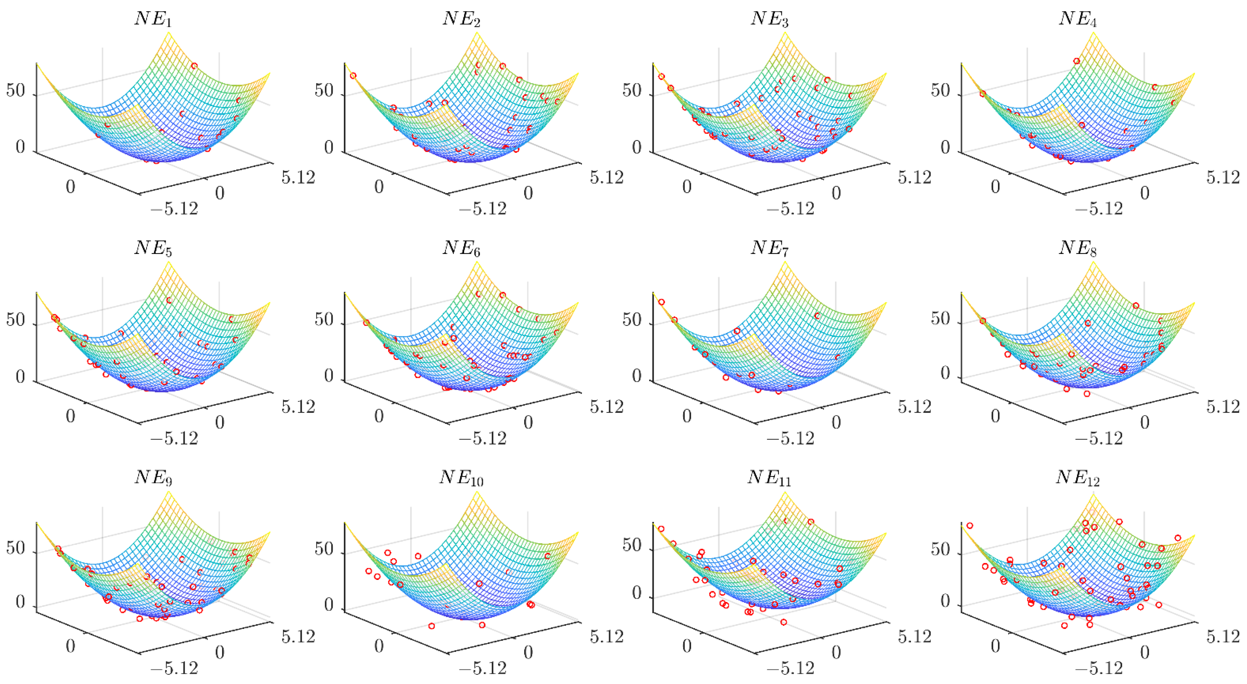
Overlarge noise probability and intensity will make the optimization problem become the problem dominated by noise that is unreasonable and meaningless. As too strong noise will not conform to the reality and too weak noise will be equated with the non-noisy environment, we set $P_n\in \left\{0,0.1,0.2,0.3\right\}$ and $SNR\in \left\{10,20,30,40,\infty \right\}$. Shown in

Table 1. Noisy environment settings.

Symbol	$\mathit{N}{\mathit{E}}_0$	$\mathit{N}{\mathit{E}}_1$	$\mathit{N}{\mathit{E}}_2$	$\mathit{N}{\mathit{E}}_3$	$\mathit{N}{\mathit{E}}_4$	$\mathit{N}{\mathit{E}}_5$	$\mathit{N}{\mathit{E}}_6$	$\mathit{N}{\mathit{E}}_7$	$\mathit{N}{\mathit{E}}_8$	$\mathit{N}{\mathit{E}}_9$	$\mathit{N}{\mathit{E}}_{10}$	$\mathit{N}{\mathit{E}}_{11}$	$\mathit{N}{\mathit{E}}_{12}$
$SNR$	$\infty$	40	40	40	30	30	30	20	20	20	10	10	10
$P_n$	0	0.1	0.2	0.3	0.1	0.2	0.3	0.1	0.2	0.3	0.1	0.2	0.3

, 12 noise levels can be obtained by combining the parameters $P_n$ and $SNR$. It should be noted that it is difficult for us to judge which parameter between noise probability and noise intensity has a greater impact on the noisy environment. Thus, we cannot compare which is noisier between the one environment $\left(P_n=0.1,SNR=10\right)$ and the other environment $\left(P_n=0.2,SNR=20\right)$. We can only make the comparison by controlling one parameter. For example, under the same noise probability, the lower the noise intensity, i.e., the greater $SNR$, the noisier the noisy environment is. Under the same noise intensity, the higher the noise probability, the noisier the noisy environment is. In addition, if noise probability is larger and noise intensity is smaller, the noisy environment will become noisier. We simulate the noisy environment based on the two-dimensional ellipsoid benchmark problem. The simulated images are shown in Figure 1. According to Figure 1, it can be found that after adding noise, the degree of disturbance is intuitively accordant with the real noise.

3.3. Benchmark Problems

Because an EA essentially is a heuristic search algorithm based on population iteration, it is difficult to prove the efficacy and performance of the algorithm through mathematical deduction. Therefore, the efficacy and performance of the EA can only be verified through a series of benchmark problems [49]. However, one risk of using benchmark problems to evaluate EAs is that the conclusions drawn from the experiment may depend on the benchmark problems being tested. To reduce this risk, the suite of benchmark problems should be both diverse and challenging. On the other hand, different types of benchmark problems have different points of concern on EAs. Using a variety of benchmark problems is also conducive to analyzing the influence of the noisy environment on DDEAs. Considering the diversity and difficulty of benchmark problems, we choose the following five benchmark problems.

• Ellipsoid

  $$F_1\left(\mathit{x}\right)={\sum }_{i=1}^{D}i\cdot x_i^2.$$

  (3)
• Rosenbrock

  $$F_2\left(\mathit{x}\right)={\sum }_{i=1}^{D-1}\left(100{\left(x_i^2-x_{i+1}\right)}^2+{\left(x_{i+1}-1\right)}^2\right).$$

  (4)
• Ackley

  $$F_3\left(\mathit{x}\right)=-20e^{-0.2\sqrt{\frac{1}{D}{\sum }_{i=1}^D{x}_i^2}}-e^{\frac{1}{D}{\sum }_{i=1}^D\cos \left(2\pi x_i\right)}+20+e.$$

  (5)
• Griewank

  $$F_4\left(\mathit{x}\right)={\sum }_{i=1}^D\frac{x_i^2}{4000}-{\prod }_{i=1}^D\cos \left(\frac{x_i}{\sqrt{i}}\right)+1.$$

  (6)
• Rastrigin

  $$F_5\left(\mathit{x}\right)={\sum }_{i=1}^D\left(x_i^2-10\cos \left(2\pi x_i\right)+10\right).$$

  (7)

The above five benchmark problems may not be the most complex problems, but they all have their own characteristics, which will be fully discussed in Section 4.4. Considering the adaptability of the selected algorithms to the dimension of the optimization problems, the dimensions of the problems are set at 10 and 30, i.e., $D\in \left\{10,30\right\}$.

4. Experiments and Analysis

In this section, we display the experimental settings and results and then analyze the experimental results in order to obtain some research conclusions. The influence of NES on DDEAs can be analyzed from three perspectives. The first is a performance comparison between DDEAs in an ideal environment (IES) and those in an NES with different levels of noise in order to find out how the noise with different levels affects the performance of DDEAs on optimization problems. The second aspect is the performance of DDEAs in IES and NES for different types of benchmark problems to find out what kind of optimization problems are slightly or significantly affected by the noise. In the third, for different DDEAs, the influence degree of NES on each algorithm is discussed to find out what kind of DDEAs are more resistant to the noise.

4.1. Experimental Settings

Most of the parameters of the DDEAs we chose are set according to their corresponding reference, except for the computational budget, or function evaluations. Online DDEAs collect new data during the optimization process, which may lead to unfair comparison between online DDEAs and offline DDEAs. For the sake of fairness, we uniformly set the computational budget $11\times D$, which is a widely used value in the research of DDEAs to test the performance of DDEAs [23,50,51,52]. It is evident that this is a reasonable setting because DDEAs are designed to be applied in environments with limited computational budgets. From the perspective of computational budget allocation, offline DDEAs allocate all the computational budget to generating the historical data, while online DDEAs allocate part or even all the computational budget to the evaluation of promising candidate solutions during the optimization process. For fairness, no special technique like the one used in [53] was used for infeasible solutions. For GPEME, infeasible solutions are replaced by the new solutions randomly generated in the domain. For other algorithms, the decision values of infeasible solutions are adjusted to the corresponding boundary value when they cross the border.

We tested four selected algorithms on five benchmark problems under 12 levels of NES. Because the fitness function used in the optimization process is noisy, we needed to evaluate the non-noisy fitness value of the optimal solution as the experimental results of DDEAs. In addition, the optimization results of DDEAs on five benchmark functions in the IES were considered as the results of the blank experiments. Each experiment was repeated 30 times, and the mean and standard deviation of the fitness value were recorded.

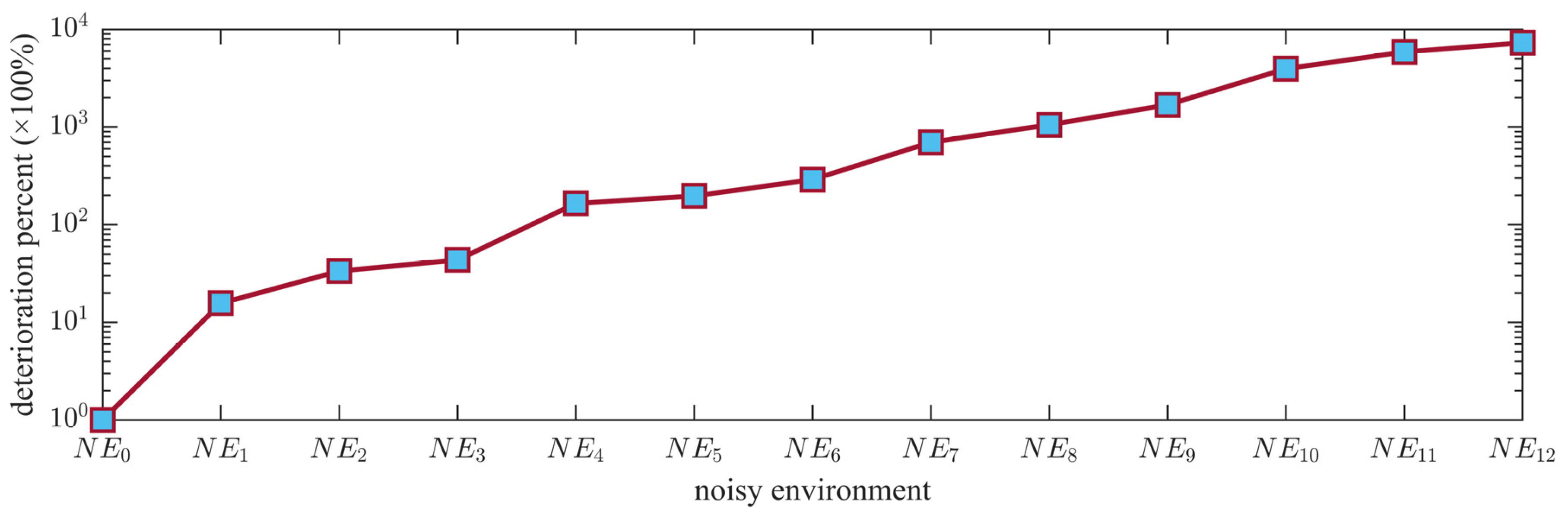
We designed the relative deterioration percent ($RDP$) index to measure the degree of difference between the final solution obtained by the same algorithm in NES ($f^{noisy}$) and that in IES ($f^{ideal}$). Its calculation formula is shown in Equation (8).

$$RDP=\frac{f^{noisy}-f^{ideal}}{f^{ideal}}\times 100\%.$$

(8)

4.2. Experimental Results

Detailed results are shown in Appendix A.

Table A1. Experimental results (with standard deviation) and relative deterioration percent ($RDP$) of DDEAs on 10-dimensional ellipsoid problems. The $RDP$ of results that significantly differ from the results obtained in non-noisy environment are shown in bold. The average rank and $p$ value are the results of the Friedman’s test with a significance level of 0.05.

Ellipsoid		$\mathit{D}=10$
$\mathit{S}\mathit{N}\mathit{R}$	${\mathit{P}}_{\mathit{n}}$	DDEA-SE	$\mathit{R}\mathit{D}\mathit{P}$	MGP-SLPSO	$\mathit{R}\mathit{D}\mathit{P}$	CAL-SAPSO	$\mathit{R}\mathit{D}\mathit{P}$	GPEME	$\mathit{R}\mathit{D}\mathit{P}$
10	0.3	2.22 ± 1.23	140.1%	1.13 × 102 ± 1.05 × 102	679.7%	7.43 × 101 ± 1.10 × 102	92,496.7%	1.49 × 102 ± 8.53 × 101	328.3%
	0.2	1.78 ± 9.97 × 10−1	92.5%	1.15 × 102 ± 9.93 × 101	691.7%	4.41 × 101 ± 8.18 × 101	54,816.7%	1.43 × 102 ± 8.36 × 101	310.8%
	0.1	1.43 ± 7.93 × 10−1	54.4%	1.03 × 102 ± 1.13 × 102	611.0%	6.40 × 101 ± 1.14 × 102	79,658.7%	1.16 × 102 ± 6.53 × 101	233.1%
20	0.3	1.15 ± 5.10 × 10−1	24.0%	4.21 × 101 ± 1.78 × 101	189.7%	6.26 ± 4.10	7696.1%	8.13 × 101 ± 3.25 × 101	133.5%
	0.2	1.14 ± 5.53 × 10−1	23.2%	3.73 × 101 ± 3.12 × 101	157.0%	6.63 ± 5.98	8153.6%	7.13 × 101 ± 3.49 × 101	104.8%
	0.1	1.09 ± 4.18 × 10−1	17.8%	4.09 × 101 ± 1.62 × 101	181.3%	7.40 ± 1.32 × 101	9122.1%	7.63 × 101 ± 3.26 × 101	119.1%
30	0.3	1.03 ± 4.13 × 10−1	11.2%	4.00 × 101 ± 1.99 × 101	175.1%	4.12 ± 3.03	5027.1%	5.21 × 101 ± 2.60 × 101	49.6%
	0.2	1.03 ± 4.28 × 10−1	11.2%	3.19 × 101 ± 1.26 × 101	119.3%	3.88 ± 2.96	4733.7%	5.42 × 101 ± 2.92 × 101	55.6%
	0.1	1.03 ± 4.03 × 10−1	11.4%	3.23 × 101 ± 1.71 × 101	122.1%	2.69 ± 2.56	3252.7%	6.20 × 101 ± 3.16 × 101	78.2%
40	0.3	1.04 ± 3.92 × 10−1	12.8%	3.87 × 101 ± 1.74 × 101	166.5%	3.43 ± 2.08	4177.6%	3.56 × 101 ± 2.15 × 101	2.1%
	0.2	1.03 ± 3.94 × 10−1	11.7%	3.06 × 101 ± 1.48 × 101	110.6%	2.84 ± 2.04	3435.2%	4.00 × 101 ± 2.34 × 101	14.9%
	0.1	1.04 ± 4.20 × 10−1	13.0%	2.30 × 101 ± 1.36 × 101	58.6%	1.24 ± 1.46	1442.6%	4.69 × 101 ± 3.24 × 101	34.6%
∞	0	9.24 × 10−1 ± 5.63 × 10−1		1.45 × 101 ± 4.57		8.03 × 10−2 ± 1.40 × 10−1		3.48 × 101 ± 1.87 × 101
Average rank		1.00		3.17		3.67		2.17
p value		NA		0.0001		0.0000		0.0269

,

Table A2. Experimental results (with standard deviation) and $RDP$ of DDEAs on 30-dimensional ellipsoid problems.

Ellipsoid		$\mathit{D}=30$
$\mathit{S}\mathit{N}\mathit{R}$	${\mathit{P}}_{\mathit{n}}$	DDEA-SE	$\mathit{R}\mathit{D}\mathit{P}$	MGP-SLPSO	$\mathit{R}\mathit{D}\mathit{P}$	CAL-SAPSO	$\mathit{R}\mathit{D}\mathit{P}$	GPEME	$\mathit{R}\mathit{D}\mathit{P}$
10	0.3	1.47 × 101 ± 5.22	264.2%	6.88 × 102 ± 2.78 × 102	28,911,903.6%	3.36 × 102 ± 4.89 × 102	12,051.6%	1.69 × 103 ± 4.82 × 102	62.0%
	0.2	1.24 × 101 ± 4.88	207.8%	5.55 × 102 ± 2.69 × 102	23,330,788.4%	1.90 × 102 ± 1.06 × 102	6790.1%	1.75 × 103 ± 6.76 × 102	67.5%
	0.1	8.75 ± 3.26	117.3%	3.73 × 102 ± 4.01 × 102	15,683,471.1%	3.10 × 102 ± 8.08 × 102	11,122.9%	1.71 × 103 ± 5.74 × 102	63.3%
20	0.3	5.33 ± 2.12	32.4%	1.60 × 102 ± 1.19 × 102	6,717,975.8%	7.04 × 101 ± 4.03 × 101	2448.9%	1.46 × 103 ± 3.12 × 102	39.3%
	0.2	5.16 ± 2.05	28.0%	9.95 × 101 ± 5.04 × 101	4,182,792.1%	6.84 × 101 ± 3.33 × 101	2376.6%	1.39 × 103 ± 3.28 × 102	33.3%
	0.1	4.58 ± 1.58	13.8%	6.59 × 101 ± 5.76 × 101	2,768,904.2%	5.64 × 101 ± 3.28 × 101	1941.8%	1.38 × 103 ± 3.85 × 102	31.5%
30	0.3	4.21 ± 1.53	4.7%	2.73 × 101 ± 2.08 × 101	1,146,046.8%	4.88 × 101 ± 1.81 × 101	1668.3%	1.32 × 103 ± 3.47 × 102	26.0%
	0.2	4.33 ± 1.56	7.6%	1.84 × 101 ± 1.79 × 101	775,467.2%	5.01 × 101 ± 2.59 × 101	1713.7%	1.21 × 103 ± 2.75 × 102	16.1%
	0.1	4.28 ± 1.55	6.3%	1.55 × 101 ± 1.58 × 101	651,070.7%	4.71 × 101 ± 2.32 × 101	1604.5%	1.17 × 103 ± 2.81 × 102	11.5%
40	0.3	4.10 ± 1.41	1.7%	3.95 ± 4.89	165,770.3%	3.85 × 101 ± 9.94	1292.3%	1.13 × 103 ± 2.98 × 102	7.7%
	0.2	4.23 ± 1.56	5.0%	3.02 ± 3.86	126,767.9%	3.67 × 101 ± 1.26 × 101	1227.0%	9.98 × 102 ± 2.79 × 102	−4.6%
	0.1	4.17 ± 1.47	3.5%	1.39 ± 2.15	58,372.0%	3.38 × 101 ± 1.50 × 101	1122.3%	9.73 × 102 ± 2.69 × 102	−7.0%
∞	0	4.03 ± 1.35		2.38 × 10−3 ± 1.74 × 10−3		2.76 ± 2.20		1.05 × 103 ± 3.12 × 102
Average rank		1.25		2.25		2.50		4.00
p value		NA		0.0578		0.0354		0.0000

,

Table A3. Experimental results (with standard deviation) and $RDP$ of DDEAs on 10-dimensional Rosenbrock problems.

Rosenbrock		$\mathit{D}=10$
$\mathit{S}\mathit{N}\mathit{R}$	${\mathit{P}}_{\mathit{n}}$	DDEA-SE	$\mathit{R}\mathit{D}\mathit{P}$	MGP-SLPSO	$\mathit{R}\mathit{D}\mathit{P}$	CAL-SAPSO	$\mathit{R}\mathit{D}\mathit{P}$	GPEME	$\mathit{R}\mathit{D}\mathit{P}$
10	0.3	2.71 × 101 ± 6.90	−4.9%	9.56 × 102 ± 8.82 × 102	350.4%	1.50 × 102 ± 1.31 × 102	711.5%	8.53 × 102 ± 4.06 × 102	445.7%
	0.2	2.67 × 101 ± 6.80	−6.6%	9.22 × 102 ± 9.02 × 102	334.4%	2.71 × 102 ± 5.98 × 102	1364.4%	9.23 × 102 ± 7.04 × 102	490.8%
	0.1	2.60 × 101 ± 5.95	−8.9%	1.01 × 103 ± 1.19 × 103	375.8%	3.67 × 102 ± 8.32 × 102	1886.6%	6.04 × 102 ± 4.91 × 102	286.8%
20	0.3	2.57 × 101 ± 6.21	−9.9%	3.34 × 102 ± 1.98 × 102	57.2%	8.44 × 101 ± 4.14 × 101	356.8%	3.94 × 102 ± 2.13 × 102	152.4%
	0.2	2.55 × 101 ± 5.88	−10.6%	2.50 × 102 ± 1.53 × 102	17.8%	8.92 × 101 ± 6.19 × 101	382.8%	3.31 × 102 ± 1.91 × 102	111.6%
	0.1	2.55 × 101 ± 5.81	−10.7%	2.05 × 102 ± 9.74 × 101	−3.3%	6.48 × 101 ± 4.08 × 101	250.7%	3.91 × 102 ± 2.57 × 102	150.4%
30	0.3	2.55 × 101 ± 5.78	−10.8%	2.12 × 102 ± 8.96 × 101	−0.3%	7.48 × 101 ± 2.66 × 101	305.0%	2.62 × 102 ± 1.21 × 102	67.8%
	0.2	2.55 × 101 ± 5.87	−10.7%	2.26 × 102 ± 9.99 × 101	6.4%	8.02 × 101 ± 5.09 × 101	334.1%	2.67 × 102 ± 1.59 × 102	71.1%
	0.1	2.53 × 101 ± 5.71	−11.2%	1.86 × 102 ± 7.64 × 101	−12.4%	6.49 × 101 ± 3.72 × 101	251.4%	2.70 × 102 ± 1.50 × 102	72.5%
40	0.3	2.54 × 101 ± 5.67	−11.0%	1.96 × 102 ± 8.00 × 101	−7.5%	5.96 × 101 ± 2.44 × 101	222.8%	1.84 × 102 ± 9.23 × 101	18.0%
	0.2	2.54 × 101 ± 5.84	−11.0%	2.23 × 102 ± 1.25 × 102	5.2%	5.85 × 101 ± 1.97 × 101	216.5%	1.38 × 102 ± 7.10 × 101	−11.5%
	0.1	2.53 × 101 ± 5.69	−11.2%	1.74 × 102 ± 6.19 × 101	−18.3%	4.11 × 101 ± 2.30 × 101	122.5%	1.69 × 102 ± 9.44 × 101	8.4%
∞	0	2.85 × 101 ± 7.74		2.12 × 102 ± 9.47 × 101		1.85 × 101 ± 7.25		1.56 × 102 ± 8.00 × 101
Average rank		1.00		3.42		2.00		3.58
p value		NA		0.0000		0.0578		0.0000

,

Table A4. Experimental results (with standard deviation) and $RDP$ of DDEAs on 30-dimensional Rosenbrock problems.

Rosenbrock		$\mathit{D}=30$
$\mathit{S}\mathit{N}\mathit{R}$	${\mathit{P}}_{\mathit{n}}$	DDEA-SE	$\mathit{R}\mathit{D}\mathit{P}$	MGP-SLPSO	$\mathit{R}\mathit{D}\mathit{P}$	CAL-SAPSO	$\mathit{R}\mathit{D}\mathit{P}$	GPEME	$\mathit{R}\mathit{D}\mathit{P}$
10	0.3	6.36 × 101 ± 6.86	11.5%	1.74 × 103 ± 1.17 × 103	1341.8%	3.13 × 102 ± 1.76 × 102	491.3%	4.43 × 103 ± 1.79 × 103	181.8%
	0.2	6.16 × 101 ± 7.35	8.1%	1.48 × 103 ± 8.96 × 102	1128.2%	2.60 × 102 ± 1.19 × 102	390.9%	3.74 × 103 ± 1.59 × 103	137.8%
	0.1	5.85 × 101 ± 6.35	2.8%	1.18 × 103 ± 1.02 × 103	876.1%	3.83 × 102 ± 3.07 × 102	623.2%	3.73 × 103 ± 1.81 × 103	137.3%
20	0.3	5.79 × 101 ± 5.23	1.7%	6.35 × 102 ± 3.87 × 102	425.7%	3.09 × 102 ± 1.65 × 102	483.5%	3.10 × 103 ± 8.82 × 102	97.1%
	0.2	5.75 × 101 ± 5.24	1.0%	5.42 × 102 ± 2.72 × 102	348.7%	2.95 × 102 ± 1.30 × 102	456.9%	3.21 × 103 ± 7.97 × 102	104.3%
	0.1	5.71 × 101 ± 5.19	0.2%	5.92 × 102 ± 2.77 × 102	390.2%	3.17 × 102 ± 2.01 × 102	499.3%	3.02 × 103 ± 1.06 × 103	92.0%
30	0.3	5.72 × 101 ± 4.75	0.4%	3.77 × 102 ± 1.53 × 102	211.7%	3.04 × 102 ± 1.38 × 102	474.3%	2.47 × 103 ± 5.97 × 102	56.6%
	0.2	5.69 × 101 ± 4.74	−0.1%	3.04 × 102 ± 8.69 × 101	151.7%	3.26 × 102 ± 1.56 × 102	516.2%	2.61 × 103 ± 7.16 × 102	66.1%
	0.1	5.68 × 101 ± 5.09	−0.4%	2.72 × 102 ± 1.01 × 102	124.8%	2.60 × 102 ± 1.55 × 102	391.0%	2.48 × 103 ± 8.11 × 102	57.3%
40	0.3	5.69 × 101 ± 4.63	−0.2%	1.98 × 102 ± 4.33 × 101	64.0%	1.84 × 102 ± 6.16 × 101	246.9%	2.16 × 103 ± 5.75 × 102	37.3%
	0.2	5.71 × 101 ± 5.17	0.2%	2.29 × 102 ± 6.38 × 101	89.6%	1.74 × 102 ± 5.38 × 101	228.9%	1.93 × 103 ± 8.06 × 102	22.5%
	0.1	5.70 × 101 ± 4.82	0.0%	1.99 × 102 ± 7.25 × 101	64.4%	1.44 × 102 ± 5.97 × 101	172.5%	1.92 × 103 ± 6.25 × 102	21.7%
∞	0	5.70 × 101 ± 4.64		1.21 × 102 ± 2.21 × 101		5.29 × 101 ± 8.96		1.57 × 103 ± 4.29 × 102
Average rank		1.00		2.92		2.08		4.00
p value		NA		0.0006		0.0398		0.0000

,

Table A5. Experimental results (with standard deviation) and $RDP$ of DDEAs on 10-dimensional Ackley problems.

Ackley		$\mathit{D}=10$
$\mathit{S}\mathit{N}\mathit{R}$	${\mathit{P}}_{\mathit{n}}$	DDEA-SE	$\mathit{R}\mathit{D}\mathit{P}$	MGP-SLPSO	$\mathit{R}\mathit{D}\mathit{P}$	CAL-SAPSO	$\mathit{R}\mathit{D}\mathit{P}$	GPEME	$\mathit{R}\mathit{D}\mathit{P}$
10	0.3	1.70 × 101 ± 2.52	202.6%	2.10 × 101 ± 5.49 × 10−1	32.1%	2.14 × 101 ± 3.98 × 10−1	13.7%	2.12 × 101 ± 3.85 × 10−1	36.2%
	0.2	1.68 × 101 ± 2.40	199.8%	2.10 × 101 ± 8.76 × 10−1	31.8%	2.12 × 101 ± 5.87 × 10−1	12.7%	2.07 × 101 ± 9.79 × 10−1	32.9%
	0.1	1.60 × 101 ± 3.11	184.3%	2.12 × 101 ± 4.60 × 10−1	33.0%	2.13 × 101 ± 4.79 × 10−1	13.2%	2.03 × 101 ± 1.83	30.6%
20	0.3	1.23 × 101 ± 2.62	119.5%	2.09 × 101 ± 7.55 × 10−1	31.1%	2.12 × 101 ± 5.83 × 10−1	12.6%	1.90 × 101 ± 3.35	21.9%
	0.2	1.15 × 101 ± 2.09	105.4%	1.94 × 101 ± 1.99	22.0%	2.09 × 101 ± 9.29 × 10−1	11.1%	1.86 × 101 ± 3.10	19.0%
	0.1	1.01 × 101 ± 2.12	79.4%	1.84 × 101 ± 2.17	15.8%	2.09 × 101 ± 9.29 × 10−1	10.9%	1.87 × 101 ± 2.54	19.8%
30	0.3	7.32 ± 1.53	30.1%	1.63 × 101 ± 2.10	2.8%	1.99 × 101 ± 7.58 × 10−1	5.4%	1.68 × 101 ± 2.70	7.6%
	0.2	6.89 ± 1.07	22.6%	1.65 × 101 ± 1.56	3.4%	1.98 × 101 ± 9.18 × 10−1	5.0%	1.65 × 101 ± 3.14	6.2%
	0.1	6.35 ± 1.09	12.9%	1.63 × 101 ± 1.73	2.8%	1.97 × 101 ± 8.77 × 10−1	4.6%	1.60 × 101 ± 3.09	2.4%
40	0.3	5.80 ± 1.10	3.2%	1.57 × 101 ± 1.65	−1.4%	1.94 × 101 ± 9.02 × 10−1	2.7%	1.69 × 101 ± 2.76	8.3%
	0.2	5.77 ± 9.51 × 10−1	2.6%	1.54 × 101 ± 1.76	−3.1%	1.91 × 101 ± 8.77 × 10−1	1.6%	1.62 × 101 ± 3.13	3.7%
	0.1	5.67 ± 9.77 × 10−1	0.9%	1.56 × 101 ± 1.76	−2.2%	1.93 × 101 ± 6.55 × 10−1	2.3%	1.61 × 101 ± 3.23	3.2%
∞	0	5.62 ± 8.75 × 10−1		1.59 × 101 ± 1.39		1.88 × 101 ± 1.26		1.56 × 101 ± 3.09
Average rank		1.00		2.42		4.00		2.58
p value		NA		0.0072		0.0000		0.0053

,

Table A6. Experimental results (with standard deviation) and $RDP$ of DDEAs on 30-dimensional Ackley problems.

Ackley		$\mathit{D}=30$
$\mathit{S}\mathit{N}\mathit{R}$	${\mathit{P}}_{\mathit{n}}$	DDEA-SE	$\mathit{R}\mathit{D}\mathit{P}$	MGP-SLPSO	$\mathit{R}\mathit{D}\mathit{P}$	CAL-SAPSO	$\mathit{R}\mathit{D}\mathit{P}$	GPEME	$\mathit{R}\mathit{D}\mathit{P}$
10	0.3	1.69 × 101 ± 1.77	253.5%	2.08 × 101 ± 4.22 × 10−1	110.0%	2.15 × 101 ± 2.98 × 10−1	47.2%	2.11 × 101 ± 3.21 × 10−1	13.7%
	0.2	1.68 × 101 ± 1.97	251.9%	2.09 × 101 ± 3.93 × 10−1	110.6%	2.13 × 101 ± 3.67 × 10−1	46.2%	2.10 × 101 ± 4.46 × 10−1	13.5%
	0.1	1.61 × 101 ± 2.30	237.7%	2.08 × 101 ± 4.67 × 10−1	109.6%	2.14 × 101 ± 4.52 × 10−1	46.6%	2.09 × 101 ± 7.85 × 10−1	12.9%
20	0.3	1.39 × 101 ± 1.95	191.6%	2.03 × 101 ± 7.13 × 10−1	104.3%	2.14 × 101 ± 3.13 × 10−1	46.5%	2.09 × 101 ± 5.47 × 10−1	12.5%
	0.2	1.33 × 101 ± 1.94	178.5%	1.97 × 101 ± 1.52	98.5%	2.13 × 101 ± 3.39 × 10−1	45.8%	2.05 × 101 ± 9.79 × 10−1	10.8%
	0.1	1.18 × 101 ± 1.95	146.6%	1.78 × 101 ± 2.55	79.0%	2.12 × 101 ± 8.36 × 10−1	45.5%	2.06 × 101 ± 7.70 × 10−1	11.2%
30	0.3	8.66 ± 1.15	81.1%	1.40 × 101 ± 2.28	40.6%	2.06 × 101 ± 9.25 × 10−1	41.3%	1.95 × 101 ± 1.10	5.4%
	0.2	7.99 ± 1.13	67.1%	1.42 × 101 ± 2.44	43.1%	2.00 × 101 ± 1.66	37.1%	1.95 × 101 ± 7.37 × 10−1	5.2%
	0.1	6.82 ± 9.83 × 10−1	42.7%	1.27 × 101 ± 1.96	28.0%	1.94 × 101 ± 1.64	33.3%	1.94 × 101 ± 1.04	4.7%
40	0.3	5.52 ± 5.87 × 10−1	15.4%	1.17 × 101 ± 2.52	17.7%	1.75 × 101 ± 1.86	20.1%	1.92 × 101 ± 9.18 × 10−1	3.7%
	0.2	5.29 ± 5.10 × 10−1	10.6%	1.04 × 101 ± 2.04	5.0%	1.63 × 101 ± 2.64	12.0%	1.88 × 101 ± 1.05	1.6%
	0.1	5.06 ± 6.01 × 10−1	5.8%	1.01 × 101 ± 2.44	1.3%	1.65 × 101 ± 2.12	12.9%	1.93 × 101 ± 6.99 × 10−1	4.1%
∞	0	4.78 ± 3.58 × 10−1		9.93 ± 2.51		1.46 × 101 ± 2.38		1.85 × 101 ± 1.07
Average rank		1.00		2.00		3.75		3.25
p value		NA		0.0578		0.0000		0.0000

,

Table A7. Experimental results (with standard deviation) and $RDP$ of DDEAs on 10-dimensional Griewank problems.

Griewank		$\mathit{D}=10$
$\mathit{S}\mathit{N}\mathit{R}$	${\mathit{P}}_{\mathit{n}}$	DDEA-SE	$\mathit{R}\mathit{D}\mathit{P}$	MGP-SLPSO	$\mathit{R}\mathit{D}\mathit{P}$	CAL-SAPSO	$\mathit{R}\mathit{D}\mathit{P}$	GPEME	$\mathit{R}\mathit{D}\mathit{P}$
10	0.3	2.00 ± 6.72 × 10−1	59.3%	9.71 × 101 ± 8.69 × 101	695.1%	2.96 × 101 ± 3.28 × 101	2184.0%	1.17 × 102 ± 6.82 × 101	350.8%
	0.2	1.65 ± 4.40 × 10−1	31.5%	1.04 × 102 ± 7.78 × 101	752.3%	3.36 × 101 ± 6.44 × 101	2493.1%	9.40 × 101 ± 5.78 × 101	262.2%
	0.1	1.44 ± 2.32 × 10−1	14.8%	3.93 × 101 ± 4.54 × 101	221.8%	1.23 × 101 ± 4.10 × 101	846.5%	8.21 × 101 ± 7.50 × 101	216.3%
20	0.3	1.35 ± 1.65 × 10−1	7.2%	2.90 × 101 ± 1.13 × 101	137.8%	4.89 ± 2.84	277.5%	5.17 × 101 ± 2.80 × 101	99.2%
	0.2	1.33 ± 1.48 × 10−1	5.6%	2.90 × 101 ± 1.23 × 101	137.6%	5.38 ± 8.85	316.0%	5.86 × 101 ± 2.91 × 101	125.7%
	0.1	1.30 ± 1.50 × 10−1	3.1%	2.86 × 101 ± 1.63 × 101	134.4%	2.93 ± 2.10	126.0%	4.82 × 101 ± 2.55 × 101	85.6%
30	0.3	1.29 ± 1.30 × 10−1	2.4%	2.74 × 101 ± 1.14 × 101	124.2%	3.01 ± 1.61	132.6%	4.12 × 101 ± 1.91 × 101	58.8%
	0.2	1.28 ± 1.23 × 10−1	2.0%	2.59 × 101 ± 1.23 × 101	112.1%	2.23 ± 9.37 × 10−1	71.9%	3.84 × 101 ± 2.24 × 101	48.1%
	0.1	1.28 ± 1.44 × 10−1	1.9%	2.78 × 101 ± 1.39 × 101	127.4%	2.85 ± 2.52	120.0%	4.05 × 101 ± 2.54 × 101	55.9%
40	0.3	1.30 ± 1.62 × 10−1	3.5%	2.45 × 101 ± 1.26 × 101	100.7%	2.22 ± 7.46 × 10−1	71.2%	3.30 × 101 ± 1.89 × 101	27.3%
	0.2	1.29 ± 1.47 × 10−1	2.4%	2.54 × 101 ± 1.18 × 101	108.4%	1.85 ± 5.12 × 10−1	43.0%	2.55 × 101 ± 1.52 × 101	−1.9%
	0.1	1.28 ± 1.47 × 10−1	1.7%	2.03 × 101 ± 1.40 × 101	66.6%	2.08 ± 6.98 × 10−1	60.6%	3.13 × 101 ± 2.13 × 101	20.6%
∞	0	1.26 ± 1.39 × 10−1		1.22 × 101 ± 4.28		1.29 ± 3.04 × 10−1		2.60 × 101 ± 1.57 × 101
Average rank		1.00		3.08		2.00		3.92
p value		NA		0.0002		0.0578		0.0000

,

Table A8. Experimental results (with standard deviation) and $RDP$ of DDEAs on 30-dimensional Griewank problems.

Griewank		$\mathit{D}=30$
$\mathit{S}\mathit{N}\mathit{R}$	${\mathit{P}}_{\mathit{n}}$	DDEA-SE	$\mathit{R}\mathit{D}\mathit{P}$	MGP-SLPSO	$\mathit{R}\mathit{D}\mathit{P}$	CAL-SAPSO	$\mathit{R}\mathit{D}\mathit{P}$	GPEME	$\mathit{R}\mathit{D}\mathit{P}$
10	0.3	4.49 ± 1.18	263.5%	1.70 × 102 ± 8.61 × 101	137,681.1%	7.42 × 101 ± 1.38 × 102	5103.3%	4.37 × 102 ± 1.42 × 102	80.9%
	0.2	3.37 ± 5.68 × 10−1	172.9%	1.04 × 102 ± 6.41 × 101	84,725.9%	8.23 × 101 ± 1.82 × 102	5665.5%	3.94 × 102 ± 1.31 × 102	63.3%
	0.1	2.33 ± 4.33 × 10−1	88.6%	6.10 × 101 ± 3.98 × 101	49,390.6%	4.07 × 101 ± 1.18 × 102	2751.2%	4.14 × 102 ± 1.82 × 102	71.5%
20	0.3	1.59 ± 1.77 × 10−1	29.2%	2.37 × 101 ± 1.89 × 101	19,106.1%	1.09 × 101 ± 6.29	660.7%	3.55 × 102 ± 7.64 × 101	47.1%
	0.2	1.47 ± 1.10 × 10−1	19.5%	2.61 × 101 ± 3.62 × 101	21,089.5%	6.21 ± 2.36	335.4%	3.46 × 102 ± 7.45 × 101	43.4%
	0.1	1.37 ± 1.08 × 10−1	10.9%	1.13 × 101 ± 8.03	9100.3%	7.14 ± 4.33	400.5%	3.21 × 102 ± 6.66 × 101	33.1%
30	0.3	1.29 ± 1.21 × 10−1	4.2%	5.61 ± 6.26	4455.6%	5.86 ± 2.61	311.0%	3.04 × 102 ± 5.74 × 101	25.8%
	0.2	1.26 ± 8.30 × 10−2	2.2%	4.40 ± 2.79	3473.8%	5.18 ± 2.07	262.9%	2.98 × 102 ± 6.25 × 101	23.5%
	0.1	1.27 ± 1.00 × 10−1	2.7%	3.54 ± 3.30	2772.2%	5.59 ± 3.59	291.6%	2.66 × 102 ± 5.09 × 101	10.3%
40	0.3	1.25 ± 8.76 × 10−2	1.0%	1.97 ± 1.18	1501.6%	5.56 ± 2.66	289.7%	2.28 × 102 ± 4.22 × 101	−5.6%
	0.2	1.23 ± 8.68 × 10−2	−0.2%	1.80 ± 1.45	1357.4%	4.82 ± 2.02	238.0%	2.54 × 102 ± 6.25 × 101	5.1%
	0.1	1.24 ± 8.58 × 10−2	0.7%	1.28 ± 5.52 × 10−1	935.6%	4.42 ± 2.90	209.7%	2.35 × 102 ± 6.01 × 101	−2.7%
∞	0	1.23 ± 9.43 × 10−2		1.23 × 10−1 ± 4.84 × 10−2		1.43 ± 1.21 × 10−1		2.41 × 102 ± 6.24 × 101
Average rank		1.00		2.50		2.50		4.00
p value		NA		0.0044		0.0044		0.0000

,

Table A9. Experimental results (with standard deviation) and $RDP$ of DDEAs on 10-dimensional Rastrigin problems.

Rastrigin		$\mathit{D}=10$
$\mathit{S}\mathit{N}\mathit{R}$	${\mathit{P}}_{\mathit{n}}$	DDEA-SE	$\mathit{R}\mathit{D}\mathit{P}$	MGP-SLPSO	$\mathit{R}\mathit{D}\mathit{P}$	CAL-SAPSO	$\mathit{R}\mathit{D}\mathit{P}$	GPEME	$\mathit{R}\mathit{D}\mathit{P}$
10	0.3	8.82 × 101 ± 2.06 × 101	54.3%	1.37 × 102 ± 3.30 × 101	51.7%	1.48 × 102 ± 3.27 × 101	104.8%	1.25 × 102 ± 2.10 × 101	101.7%
	0.2	7.77 × 101 ± 2.51 × 101	36.0%	1.30 × 102 ± 3.12 × 101	44.8%	1.41 × 102 ± 3.25 × 101	95.0%	1.49 × 102 ± 4.15 × 101	140.7%
	0.1	7.23 × 101 ± 2.59 × 101	26.6%	1.31 × 102 ± 4.59 × 101	45.9%	1.33 × 102 ± 4.24 × 101	84.1%	1.14 × 102 ± 4.07 × 101	84.2%
20	0.3	6.16 × 101 ± 2.02 × 101	7.8%	9.18 × 101 ± 1.79 × 101	2.0%	1.08 × 102 ± 1.47 × 101	49.1%	8.60 × 101 ± 1.92 × 101	38.7%
	0.2	5.53 × 101 ± 2.05 × 101	−3.2%	9.59 × 101 ± 1.80 × 101	6.4%	1.01 × 102 ± 1.83 × 101	39.9%	7.13 × 101 ± 2.16 × 101	15.1%
	0.1	5.30 × 101 ± 2.10 × 101	−7.2%	8.64 × 101 ± 1.40 × 101	−4.0%	9.55 × 101 ± 2.51 × 101	31.9%	7.49 × 101 ± 1.94 × 101	20.8%
30	0.3	5.02 × 101 ± 1.91 × 101	−12.2%	8.87 × 101 ± 1.49 × 101	−1.5%	8.88 × 101 ± 2.38 × 101	22.7%	6.76 × 101 ± 1.88 × 101	9.0%
	0.2	4.87 × 101 ± 1.86 × 101	−14.8%	8.95 × 101 ± 1.28 × 101	−0.7%	8.67 × 101 ± 2.34 × 101	19.8%	6.39 × 101 ± 1.79 × 101	3.0%
	0.1	4.79 × 101 ± 1.77 × 101	−16.1%	8.56 × 101 ± 1.53 × 101	−4.9%	8.40 × 101 ± 2.56 × 101	16.0%	6.95 × 101 ± 1.48 × 101	12.2%
40	0.3	4.83 × 101 ± 2.00 × 101	−15.4%	8.37 × 101 ± 1.32 × 101	−7.1%	8.64 × 101 ± 2.74 × 101	19.3%	6.04 × 101 ± 1.59 × 101	−2.6%
	0.2	4.97 × 101 ± 1.80 × 101	−13.0%	8.84 × 101 ± 1.05 × 101	−1.8%	8.63 × 101 ± 2.70 × 101	19.2%	5.96 × 101 ± 9.95	−3.9%
	0.1	4.76 × 101 ± 1.79 × 101	−16.7%	8.47 × 101 ± 1.54 × 101	−6.0%	8.48 × 101 ± 2.40 × 101	17.1%	6.59 × 101 ± 1.77 × 101	6.4%
∞	0	5.71 × 101 ± 1.96 × 101		9.01 × 101 ± 1.15 × 101		7.24 × 101 ± 3.15 × 101		6.20 × 101 ± 1.41 × 101
Average rank		1.00		3.17		3.67		2.17
p value		NA		0.0001		0.0000		0.0269

and

Table A10. Experimental results (with standard deviation) and $RDP$ of DDEAs on 30-dimensional Rastrigin problems.

Rastrigin		$\mathit{D}=30$
$\mathit{S}\mathit{N}\mathit{R}$	${\mathit{P}}_{\mathit{n}}$	DDEA-SE	$\mathit{R}\mathit{D}\mathit{P}$	MGP-SLPSO	$\mathit{R}\mathit{D}\mathit{P}$	CAL-SAPSO	$\mathit{R}\mathit{D}\mathit{P}$	GPEME	$\mathit{R}\mathit{D}\mathit{P}$
10	0.3	2.90 × 102 ± 4.59 × 101	164.4%	4.06 × 102 ± 4.41 × 101	85.5%	4.57 × 102 ± 8.59 × 101	1129.7%	4.60 × 102 ± 6.49 × 101	74.0%
	0.2	2.80 × 102 ± 3.85 × 101	154.7%	3.88 × 102 ± 5.46 × 101	77.5%	4.48 × 102 ± 8.10 × 101	1105.0%	4.35 × 102 ± 8.08 × 101	64.9%
	0.1	2.26 × 102 ± 5.76 × 101	105.6%	3.73 × 102 ± 5.03 × 101	70.7%	4.18 × 102 ± 1.08 × 102	1025.1%	4.43 × 102 ± 8.22 × 101	67.7%
20	0.3	1.56 × 102 ± 3.84 × 101	41.6%	3.08 × 102 ± 3.89 × 101	41.1%	2.66 × 102 ± 5.43 × 101	616.1%	3.48 × 102 ± 4.36 × 101	31.9%
	0.2	1.44 × 102 ± 3.61 × 101	31.5%	2.96 × 102 ± 4.72 × 101	35.3%	2.37 × 102 ± 4.16 × 101	536.6%	3.50 × 102 ± 5.93 × 101	32.7%
	0.1	1.28 × 102 ± 3.57 × 101	16.2%	2.62 × 102 ± 3.96 × 101	20.1%	2.12 × 102 ± 6.09 × 101	469.4%	3.32 × 102 ± 6.39 × 101	25.7%
30	0.3	1.15 × 102 ± 3.20 × 101	5.1%	2.21 × 102 ± 2.80 × 101	0.9%	1.46 × 102 ± 4.38 × 101	292.0%	3.01 × 102 ± 3.96 × 101	13.9%
	0.2	1.14 × 102 ± 3.23 × 101	4.1%	2.19 × 102 ± 2.89 × 101	0.2%	1.16 × 102 ± 4.15 × 101	210.8%	2.93 × 102 ± 4.51 × 101	11.0%
	0.1	1.14 × 102 ± 3.10 × 101	4.2%	2.29 × 102 ± 1.97 × 101	4.7%	9.23 × 101 ± 4.07 × 101	148.1%	2.86 × 102 ± 3.65 × 101	8.1%
40	0.3	1.14 × 102 ± 2.93 × 101	3.5%	2.24 × 102 ± 1.96 × 101	2.5%	6.76 × 101 ± 2.74 × 101	81.7%	2.76 × 102 ± 4.28 × 101	4.5%
	0.2	1.12 × 102 ± 3.20 × 101	2.2%	2.25 × 102 ± 2.76 × 101	3.1%	5.23 × 101 ± 1.90 × 101	40.6%	2.55 × 102 ± 4.88 × 101	−3.3%
	0.1	1.13 × 102 ± 3.08 × 101	3.2%	2.21 × 102 ± 2.85 × 101	1.3%	5.53 × 101 ± 1.98 × 101	48.7%	2.67 × 102 ± 3.32 × 101	1.0%
∞	0	1.10 × 102 ± 2.90 × 101		2.19 × 102 ± 3.00 × 101		3.72 × 101 ± 1.85 × 101		2.64 × 102 ± 3.82 × 101
Average rank		1.33		2.75		2.00		3.92
p value		NA		0.0144		0.2059		0.0000

show the real fitness value and the $RDP$ value of the final solution obtained by the four test algorithms, respectively. We utilized the Wilcoxon rank-sum test to determine whether the results obtained in NES were significantly different from the results obtained in IES. The hypothesis was that the overall distributions of the results obtained in IES and in NES of a certain noisy level would be the same. If the rank-sum test result was smaller than the significant level 0.05, the hypothesis would be rejected. Meanwhile, the $RDP$ of results that significantly differ from the results obtained in IES are shown in bold in Table A1, Table A2, Table A3, Table A4, Table A5, Table A6, Table A7, Table A8, Table A9 and Table A10. When comparing the optimization results of four algorithms in NES, the Friedman’s test with a significance level of 0.05 was adopted. The Friedman’s test result $p$ value is shown in Table A1, Table A2, Table A3, Table A4, Table A5, Table A6, Table A7, Table A8, Table A9 and Table A10.

4.3. Effect of Noise Levels

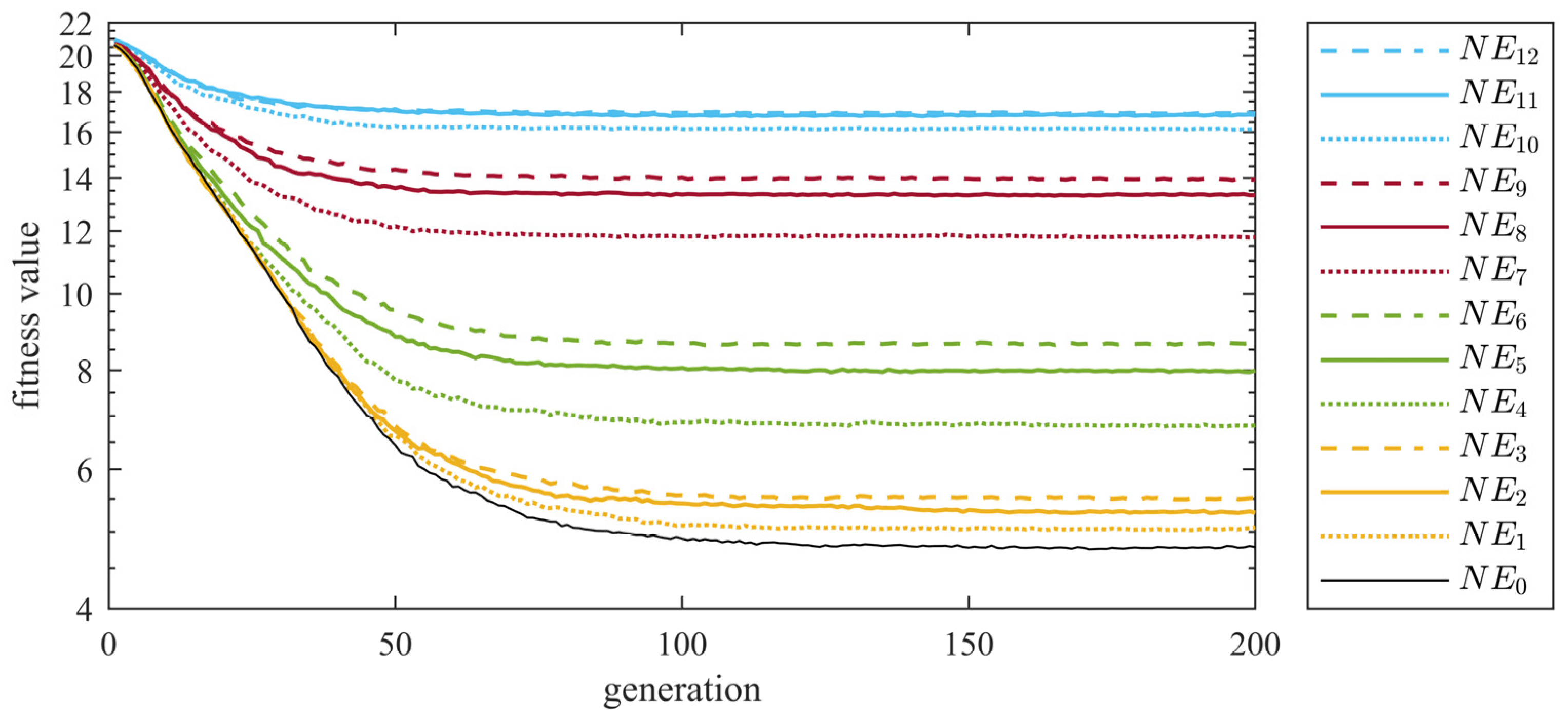
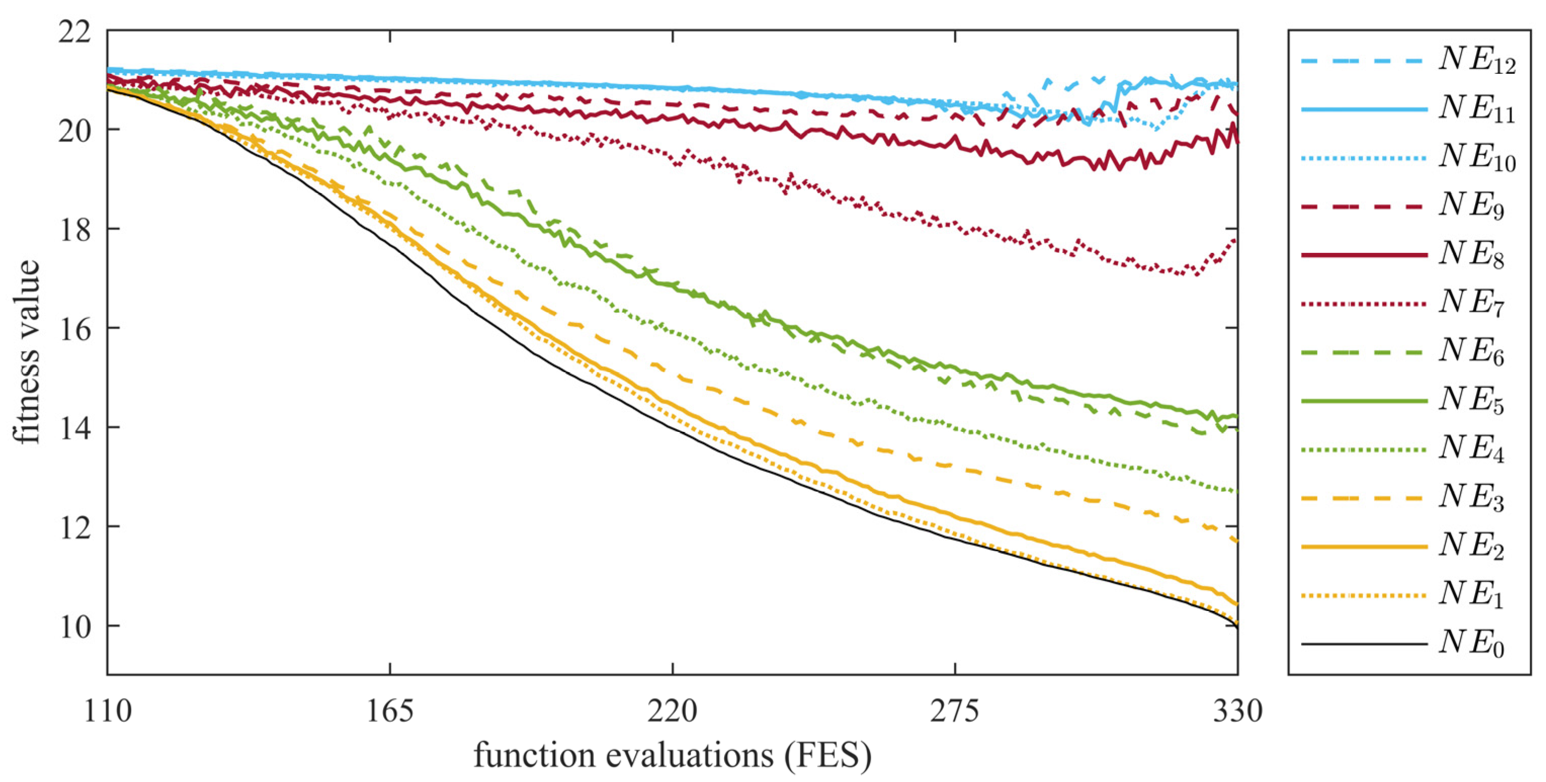
As shown in Figure 2, the performance of DDEAs was not very sensitive when the environment was posed with low-level noises. This owes much to the liberal search behaviors of the population-based EAs, which are not as greedy/directional as the traditional gradient-based or single solution-based optimizers. However, with the rising noise levels, the results of the tested DDEAs showed deterioration. The deterioration is mainly reflected in two aspects. One is the mean value of the optimization results; the other is the standard deviation. For detail analysis, we take the experiment of DDEA-SE being tested on the 30-dimensional Ackley problem as the example (as other results in the Appendix A also show similar conclusions). The experimental results are shown in

Table 2. Experimental results of DDEA-SE on 30-dimensional Ackley problems.

	$\mathit{S}\mathit{N}\mathit{R}$	${\mathit{P}}_{\mathit{n}}$	Mean	std	$\mathit{R}\mathit{D}\mathit{P}$
$N{E}_{12}$	10	0.3	1.69 × 101	1.77	253.5%
$N{E}_{11}$		0.2	1.68 × 101	1.97	251.9%
$N{E}_{10}$		0.1	1.61 × 101	2.30	237.7%
$N{E}_9$	20	0.3	1.39 × 101	1.95	191.6%
$N{E}_8$		0.2	1.33 × 101	1.94	178.5%
$N{E}_7$		0.1	1.18 × 101	1.95	146.6%
$N{E}_6$	30	0.3	8.66	1.15	81.1%
$N{E}_5$		0.2	7.99	1.13	67.1%
$N{E}_4$		0.1	6.82	9.83 × 10−1	42.7%
$N{E}_3$	40	0.3	5.52	5.87 × 10−1	15.4%
$N{E}_2$		0.2	5.29	5.10 × 10−1	10.6%
$N{E}_1$		0.1	5.06	6.01 × 10−1	5.8%
$N{E}_0$	∞	0	4.78	3.58 × 10−1	0

, and the convergence curve is shown in Figure 3. With the increase in the noise intensity (decreasing $SNR$) and increase in the noise probability $P_n$, the convergence speed of DDEA-SE decreased obviously. Meanwhile, the optimization results of DDEA-SE became worse. Owing to the disturbance of noise, DDEA-SE could only obtain a shifted optimum for the biased problem with noise influence, rather than the optimum of the original problem. Moreover, it can be seen in Table 2 that the larger the noise is, the larger the standard deviation of the optimization results will be, indicating that the convergence ability of DDEA-SE was also significantly affected.

The influence of the noise began with the disturbance of the historical data. The noisy historical data affected the mapping relationship between the variables space and the fitness space. Based on the biased mapping relationship, the accuracy and performance of the surrogate model were affected, with the consequence of increasing prediction deviation and decreasing stability. Offline DDEAs optimized the problems directly based on the biased surrogate model that had poor performance. Consequently, the obtained optimum was much worse than the optimum obtained in IES, as the optimum obtained in NES was the optimal solution of the biased benchmark problems instead of the original benchmark problems. Furthermore, online DDEAs used the biased surrogate model to search the candidate solution with the most value of being evaluated by the real fitness function. However, the search of the candidate solution could be misled; thus, the search results would be meaningless for the original problems. To make the matter worse, the evaluation of the candidate solution could be disturbed by the noise, leading to more serious deviation of the search direction.

4.4. Effect on Benchmark Problems

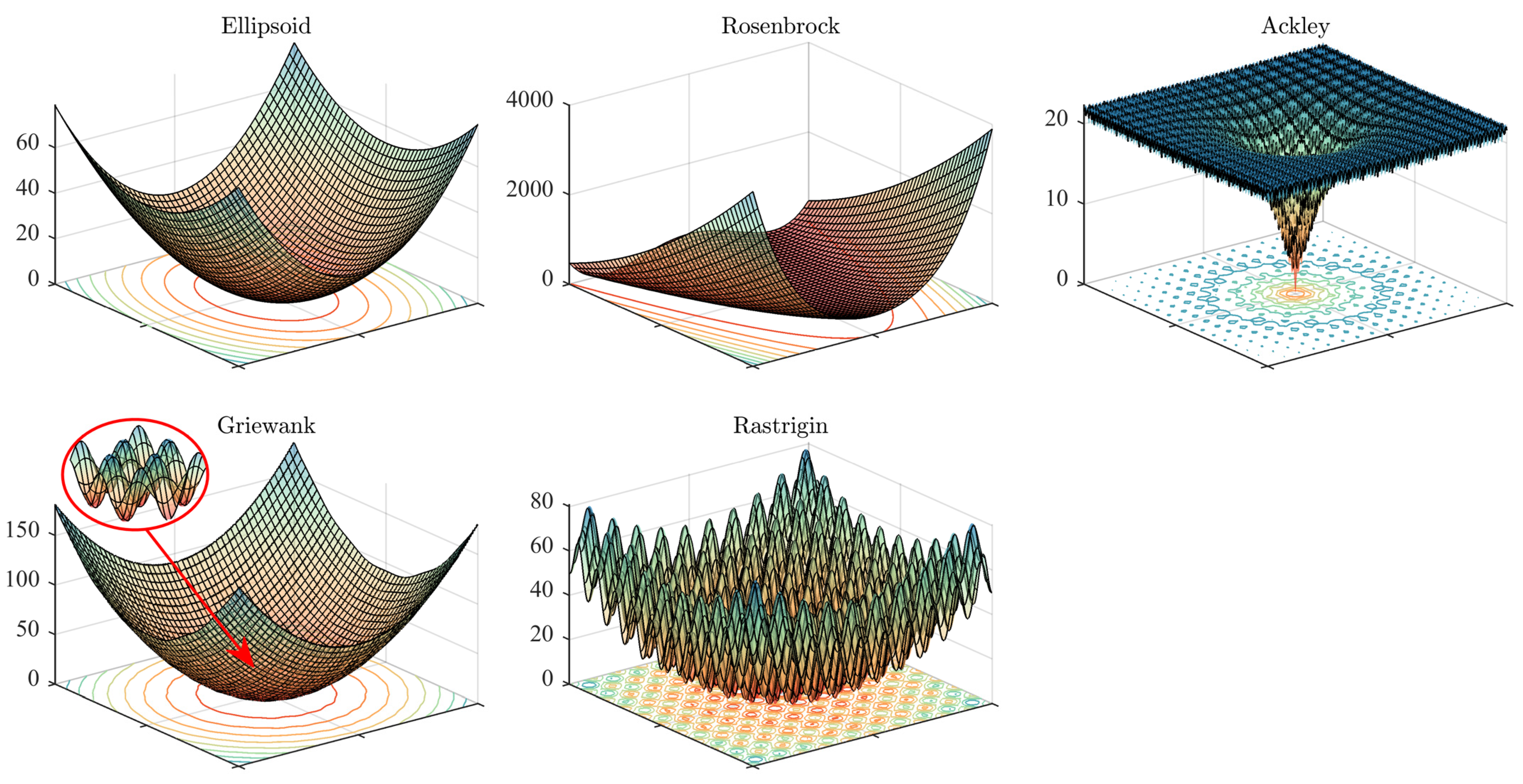
The landscape of the benchmark functions is shown in Figure 4 for the analysis. When analyzing the effect of noise level on the performance of the algorithm, some special phenomena can be found. When we tested different benchmark functions, the impact of the NES on the algorithm was significantly different. This difference was reflected in the $RDP$ value of the optimization results, as well as in the number of noise levels whose optimization results significantly differed from the results obtained in the IES. Taking DDEA-SE as an example, the related results are shown as

Table 3. Average $RDP$ of DDEA-SE on different benchmark problems in noisy environment and the number of noise levels whose optimization results are better/similar/worse than the results obtained in ideal environment.

Benchmark	$\mathit{D}$	DDEA-SE
		$\mathit{R}\mathit{D}\mathit{P}$	(+/−/≈)
Ellipsoid	10	35.28%	(0/9/3)
	30	57.69%	(0/7/5)
Rosenbrock	10	−9.79%	(0/12/0)
	30	2.10%	(0/10/2)
Ackley	10	80.27%	(0/4/8)
	30	123.53%	(0/2/10)
Griewank	10	11.29%	(0/8/4)
	30	49.60%	(0/6/6)
Rastrigin	10	2.18%	(0/9/3)
	30	44.70%	(0/6/6)

.

4.4.1. Ellipsoid

As shown in Table 3, for this benchmark, the algorithms deteriorated obviously in the NES of most noise levels. Especially in the high-dimensional case, the relative deterioration percentage was much higher than that in low-dimensional case.

Compared with other benchmark problems, the ellipsoid problem, as a unimodal function, is a very simple benchmark problem, characterized by no local optimal solution and an independent relationship among multi-dimensional variables. However, in solving the simplest benchmark problem, the interference of noise is inevitable. We can compare the landscape changes of the benchmark problem before and after adding noise. After adding noise, the originally very regular unimodal optimization problem turned into a multi-modal irregular function, which challenges the searching of EAs.

4.4.2. Rosenbrock

As shown in Table 3, the algorithm was less affected by noise in the low-dimensional case of most noise levels, which was very different from the ellipsoid problem. In the case of high dimension, the number of cases of optimization results that were affected by noise slightly increased.

In the Rosenbrock problem, the neighborhood of the global optimum is a very flat region. Hence, it is difficult for the DDEAs to accurately search the location of the global optimal solution, even though no noise is posed to the environment. However, the bright side is that, since the fitness value of the solutions near to the global optimum is very similar to the fitness value of the global optimum, if the final optimization result is located within the neighborhood domain, a good optimization result can be obtained. The addition of noise made the neighborhood domain of the global optimal solution less flat and brought a bias to the search of the evolutionary algorithm. In some noise levels of the lower dimensions cases, the bias made the final optimization results in the noisy environment even better compared with those in the non-noisy environment. In the case of higher dimensions, the phenomenon of performance enhancement decreased. This is because the Rosenbrock problem becomes more complex in higher dimensions, and a small noise can significantly change the search direction.

4.4.3. Ackley

As shown in Table 3, in the low-dimensional case, the algorithm performance was degraded by the noise, and the results of many noise levels were significantly different from those in IES. While in the high-dimensional case, the results of almost all the noise levels were significantly different from those in IES.

In contrast to the Rosenbrock problem, the Ackley problem is a function that a global optimal solution located in a steep valley. There were multiple local optimal solutions in the neighborhood field of the global optimal solution. There was a large gap between the fitness value of these local optimal solutions and the fitness of the global optimal solution. The interference of noise made the position of the searching results far away from the global optimal solution, which led to the instability and deterioration of the optimization algorithms. Even in the noisy environment with a very low noise level, the global optimal position only had a small deviation, but the response of the fitness value changed greatly.

4.4.4. Griewank

As shown in Table 3, the experimental results for the Griewank problem were very similar to the results of the ellipsoid problem. We found that the Griewank problem was a multi-peak optimization problem, but the heights of the peaks were relatively small, so the Griewank function and the Ellipsoid function were very similar roughly. Adding noise would lead to the elimination of the particularity of the benchmark problem; hence, it reduced the performance of DDEAs to a certain extent.

4.4.5. Rastrigin

As shown in Table 3, in the case of low dimension, there was no significant difference between the results of the Rastrigin problem in NES and the results in IES. At high dimension, the number of cases significantly affected by the noise increased.

The Rastrigin problem is a relatively complex problem. We know from the landscape of the problem that this problem has multiple peaks, and the height of the peaks is large. Because of the complexity of Rastrigin, the results in IES were not ideal, and the effect of noise in NES was slight.

4.4.6. Discussion

Generally, the addition of the noise changed the landscape of the optimization problems. Using the noisy data, DDEAs could only build biased surrogate models to replace the real fitness function. Guided by biased surrogate models, the searching results obtained by the DDEAs were the optimization results of the biased optimization problems. However, the quality of the optimization solution should be evaluated by the unbiased real fitness function. From the above analysis of each benchmark problem, we can generalize the relationship between the degree of noise influence and the characteristics of the benchmark problem as follows.

(1) If the landscape of the benchmark problems shows that the neighborhood of the global optimum is rugged, such as in the ellipsoid problem, the Griewank problem and the Ackley problem, the noise will have serious influences on the performance of the algorithms. This is because the original non-noisy environments of these benchmarks show strong orientation information for the EA population to search. The addition of noise blurs the orientation information and hence reduces the search efficiency of the EA population significantly.

(2) If the original landscape is very complex, containing various types of peaks, such as the Rastrigin problem, the performance degeneration by posing noise is not very prominent. The reason is twofold. On the one hand, this type of problem itself is so challenging to optimize that, even for the clean environment, the accuracy of EAs may not be very high. On the other hand, for the multimodal landscapes, there is a chance that the existence of noise diversifies the search of population and hence benefits the exploration ability of algorithms.

(3) If the problem contains a relatively flat landscape, such as the Rosenbrock problem, the noise will have the smallest influence on the performance of the DDEAs. Different from the other cases, the noise may pose additional orientation information to the flat landscape, which provides extra guidance to the EA population and hence improves the search efficiency sometimes.

4.5. Effect on Algorithms

In this section, we analyze the effect of the noise on the four DDEAs. Through the characteristics and the optimization results of the four DDEAs in IES and NES, we analyze the degree to which and the reasons that the performances of the algorithms were affected. The fitness of results in non-noisy environments and the rank of DDEAs in noisy environments are shown in

Table 4. Average fitness of DDEAs on different benchmark problems in non-noisy environments and the rank of experimental results in noisy environments. The best results are in bold.

Benchmark	$\mathit{D}$	DDEA-SE		MGP-SLPSO		CAL-SAPSO		GPEME
		Non-Noisy	Rank	Non-Noisy	Rank	Non-Noisy	Rank	Non-Noisy	Rank
Ellipsoid	10	9.24 × 10−1 ± 5.63 × 10−1	1.00	1.45 × 101 ± 4.57	3.17	8.03 × 10−2 ± 1.40 × 10−1	3.67	3.48 × 101 ± 1.87 × 101	2.17
	30	4.03 ± 1.35	1.25	2.38 × 10−3 ± 1.74 × 10−3	2.25	2.76 ± 2.20	2.50	1.05 × 103 ± 3.12 × 102	4.00
Rosenbrock	10	2.85 × 101 ± 7.74	1.00	2.12 × 102 ± 9.47 × 101	3.42	1.85 × 101 ± 7.25	2.00	1.56 × 102 ± 8.00 × 101	3.58
	30	5.70 × 101 ± 4.64	1.00	1.21 × 102 ± 2.21 × 101	2.92	5.29 × 101 ± 8.96	2.08	1.57 × 103 ± 4.29 × 102	4.00
Ackley	10	5.62 ± 8.75 × 10−1	1.00	1.59 × 101 ± 1.39	2.42	1.88 × 101 ± 1.26	4.00	1.56 × 101 ± 3.09	2.58
	30	4.78 ± 3.58 × 10−1	1.00	9.93 ± 2.51	2.00	1.46 × 101 ± 2.38	3.75	1.85 × 101 ± 1.07	3.25
Griewank	10	1.26 ± 1.39 × 10−1	1.00	1.22 × 101 ± 4.28	3.08	1.29 ± 3.04 × 10−1	2.00	2.60 × 101 ± 1.57 × 101	3.92
	30	1.23 ± 9.43 × 10−2	1.00	1.23 × 10−1 ± 4.84 × 10−2	2.50	1.43 ± 1.21 × 10−1	2.50	2.41 × 102 ± 6.24 × 101	4.00
Rastrigin	10	5.71 × 101 ± 1.96 × 101	1.00	9.01 × 101 ± 1.15 × 101	3.17	7.24 × 101 ± 3.15 × 101	3.67	6.20 × 101 ± 1.41 × 101	2.17
	30	1.10 × 102 ± 2.90 × 101	1.33	2.19 × 102 ± 3.00 × 101	2.75	3.72 × 101 ± 1.85 × 101	2.00	2.64 × 102 ± 3.82 × 101	3.92

.

4.5.1. DDEA-SE

According to Table 4, DDEA-SE, as an offline data-driven evolutionary algorithm, achieved good results in both IES and NES. Especially in NES, compared with other DDEAs, DDEA-SE showed better resistance to the noise. On the one hand, DDEA-SE used all the computational cost for the initialization of the data, and the data points affected by noise were distributed uniformly. Therefore, from the aspect of the landscape of the surrogate model, the constructed surrogate model based on these data was slightly affected. On the other hand, the idea of DDEA-SE is to approximate the benchmark problem at one time and then find the global optimum of the approximation or the surrogate model. Therefore, the part affected by the noise is only the building part of the surrogate model. Moreover, the surrogate model does not need to be completely correct. The most important key involves whether the position of the global optimal solution is shifted too much compared to the original benchmark problem. Note that DDEA-SE uses the model management strategy of selective ensemble to increase the utilization rate of data and improve the accuracy of the model.

4.5.2. MGP-SLPSO

As an online DDEA, MGP-SLPSO is designed for higher dimensional optimization problems. In the optimization of the 30-dimensional benchmark problem in IES, MGP-SLPSO was better at dealing with relatively simple benchmark problems such as the ellipsoid and Griewank problems, while its performance of other benchmark problems was not so good in terms of results. It can be seen in Figure 5, the convergence curve of MGP-SLPSO on the 30-dimensional Ackley problems, that the poor performance of the relatively complex benchmark problems was caused by the insufficient computational cost. Although MGP-SLPSO generally had a strong ability to deal with the optimization problem in IES, it was difficult to maintain that performance in NES. On the one hand, MGP-SLSPO only uses part of the computational cost for the initialization, which leads to low approximation accuracy for the benchmark problem and affects the convergence speed. On the other hand, the noise might be introduced when using the real fitness function to evaluate the candidate solutions. The distribution of these candidate solutions affected by the noise was relatively concentrated near the optimum. Therefore, the performance of the MGP-SLPSO was heavily affected by the noise because of the wrong guidance.

4.5.3. CAL-SAPSO

CAL-SAPSO is similar to MGP-SLPSO. The difference is that CAL-SAPSO uses three different kinds of surrogate models as a mixed surrogate model, which is suitable for optimization problems of medium and low dimensions. The results of CAL-SAPSO were also similar to the results of MGP-SLPSO. In IES, CAL-SAPSO also suffered from the lack of the computational cost and thus had relatively poor performance. In NES, the degree that CAL-SAPSO was affected was similar to MGP-SLPSO.

4.5.4. GPEME

GPEME is a relatively simple online DDEA compared to the other three algorithms. Correspondingly, the optimization results obtained by GPEME in IES were not good, especially in the case of high dimensions. In NES, the performance of GPEME was also relatively poor. However, the results of GPEME on the 10-dimensional ellipsoid and Rastrigin problems are better than other two online DDEAs, indicating that simple algorithms could have good performance when dealing with low-dimensional simple optimization problems.

4.5.5. Discussion

The effect of the noise on DDEAs mainly appeared in three ways. The first way was that the poor quality of the historical data led to the poor quality of the surrogate model. The noisy data interfered with the construction of the surrogate model and led to the decrease in the quality of the surrogate model. The second way was that the poor quality of the surrogate model led to the deviation of the selected global optimum or the candidate solution. Under the guidance of the surrogate model with bias, the real fitness of final or temporary results obtained could be not as good as the predicted fitness showed. The wrong selection of the candidate solution caused the waste of the computational budget or even caused the wrong searching direction. The last way was that, when evaluating the solution selected by the algorithm with predicted fitness, the interference of the noise caused the deviation of the real fitness of the solution, misleading the searching direction of the algorithm. According to the above experimental results and analysis, we can obtain some inferences as follows.

(1) The effect of the noise on online DDEAs is greater than the effect on offline DDEAs because offline DDEAs are only affected in the first way and the second way regarding the deviation of the global optimum, while online DDEAs are affected in all aspects.

(2) Building the surrogates ensemble and the selective strategy of surrogates are useful for reducing the influence of the noise.

5. Conclusions

This paper presents a comprehensive investigation of DDEAs in noisy environments which shows the impact of four representative DDEAs in NES. The main motivations of the experimental investigation were as follows: (1) The quality of data obtained in the real optimization problems is difficult to guarantee; (2) although it is known that the optimization performance of DDEAs will be affected in noisy environments, the degree of and reason for this influence have not been systematically analyzed yet.

Some significant findings to emerge from this investigation can be stated as follows:

• In this investigation, a simulation scheme for noisy data-driven optimization problems was proposed. The NES with various noise levels was constructed by controlling the noise intensity $SNR$ and the noise probability $P_n$.
• Through comparing results of DDEAs in NES and in IES, we found that, because of noise, the results of different DDEAs in NES were worse than the results in IES in most cases. Generally, the higher the noise levels in NES, the worse the performances were that the algorithms exhibited. However, there were also several special cases in which, by posing low levels of noises, the results of algorithms in NES were better than those in IES. For these cases, the existence of noise did not shift the position of optimum, meanwhile it diversified the search of the DDEA population to avoid premature convergence.
• By comparing the influence degree of noise on different benchmark problems, the relationships between the degree of noise influence and the characteristics of the benchmark problems were found. (1) During the optimization of the benchmark problem in which the neighborhood of the global optimum was rugged, the noise had serious influence on the performance of the DDEAs. (2) When the original landscape of the problem was very complex with various types of peaks, the performance degeneration by posing noise was not as prominent. (3) If the problem contained a relatively flat landscape, the noise had the smallest influence on the DDEAs.
• According to the optimization results of different DDEAs, it was found that the offline DDEAs had stronger resistance to noise than online DDEAs. Meanwhile, the ensemble and the selection strategies of surrogates were helpful in NES.
• The effects of the noise on DDEAs occurred as follows: (1) For the online DDEAs, noise affected the surrogates and then affected the selection of candidate solutions which would then be evaluated by the real fitness function. Meanwhile, the noise could be introduced during the evaluation of promising solutions, which would further affect the search of the algorithms. (2) For the offline DDEA, the noise appeared in the historical data and then affected the performance of the surrogate model, resulting in the shift of the global optimum.

This study shows the influences on DDEAs in noisy environments and the reasons for these influences. Based on the above observation, we found that when solving real-world optimization problems in the noisy environment, if data-driven evolutionary algorithms are used, offline DDEAs are more preferred than online DDEAs, and for online DDEAs, it is recommendable to assign as large a computational budget as possible to acquire historical data and train the surrogate.

This study indicates that there are several promising directions for future research:

• So far, the existing DDEAs are all developed and tested for the ideal environment. In the future, it is appealing to study the data-driven optimization in noisy environments, as well as to explore the DDEAs with stronger noise resistance.
• The current studies of DDEAs have not yet paid attention to carrying out preprocessing on the data. In the data-mining area, preprocessing has always been a simple but effective scheme to reduce the impact of noise. Therefore, based on this research work, the performance of DDEAs in noisy environments after preprocessing the data can be further investigated, and the influence of preprocessing on DDEAs in noisy environments can be studied.

References

- Jin, Y.; Wang, H.; Chugh, T.; Guo, D.; Miettinen, K. Data-Driven Evolutionary Optimization: An Overview and Case Studies. IEEE Trans. Evol. Comput. 2019, 23, 442–458. [Google Scholar] [CrossRef]
- Wu, Z.; Yu, S.; Li, T. A Meta-Model-Based Multi-Objective Evolutionary Approach to Robust Job Shop Scheduling. Mathematics 2019, 7, 529. [Google Scholar] [CrossRef] [Green Version]
- Yao, X. Evolving Artificial Neural Networks. Proc. IEEE 1999, 87, 1423–1447. [Google Scholar]
- Yao, X.; Liu, Y. A New Evolutionary System for Evolving Artificial Neural Networks. IEEE Trans. Neural Netw. 1997, 8, 694–713. [Google Scholar] [CrossRef] [Green Version]
- Wang, H.; Jin, Y.; Jansen, J.O. Data-Driven Surrogate-Assisted Multiobjective Evolutionary Optimization of a Trauma System. IEEE Trans. Evol. Comput. 2016, 20, 939–952. [Google Scholar] [CrossRef] [Green Version]
- Liu, Y.; Shang, F.; Jiao, L.; Cheng, J.; Cheng, H. Trace Norm Regularized CANDECOMP/PARAFAC Decomposition with Missing Data. IEEE Trans. Cybern. 2015, 45, 2437–2448. [Google Scholar] [CrossRef]
- Wang, S.; Yao, X. Multiclass Imbalance Problems: Analysis and Potential Solutions. IEEE Trans. Syst. Man Cybern. Part B (Cybern.) 2012, 42, 1119–1130. [Google Scholar] [CrossRef]
- Wang, S.; Minku, L.L.; Yao, X. Resampling-Based Ensemble Methods for Online Class Imbalance Learning. IEEE Trans. Knowl. Data Eng. 2015, 27, 1356–1368. [Google Scholar] [CrossRef] [Green Version]
- Gao, Y.; Wang, K.; Gao, C.; Shen, Y.; Li, T. Application of Differential Evolution Algorithm Based on Mixed Penalty Function Screening Criterion in Imbalanced Data Integration Classification. Mathematics 2019, 7, 1237. [Google Scholar] [CrossRef] [Green Version]
- Wang, H.; Zhang, Q.; Jiao, L.; Yao, X. Regularity Model for Noisy Multiobjective Optimization. IEEE Trans. Cybern. 2016, 46, 1997–2009. [Google Scholar] [CrossRef] [Green Version]
- Beyer, H.-G. Evolutionary Algorithms in Noisy Environments: Theoretical Issues and Guidelines for Practice. Comput. Methods Appl. Mech. Eng. 2000, 186, 239–267. [Google Scholar] [CrossRef]
- Nissen, V.; Propach, J. On the Robustness of Population-Based versus Point-Based Optimization in the Presence of Noise. IEEE Trans. Evol. Comput. 1998, 2, 107–119. [Google Scholar] [CrossRef]
- Arnold, D.V.; Beyer, H.-G. Noisy Optimization with Evolution Strategies; Springer Science & Business Media: Berlin/Heidelberg, Germany, 2002. [Google Scholar]
- Arnold, D.V. Evolution Strategies in Noisy Environments—A Survey of Existing Work. In Theoretical Aspects of Evolutionary Computing; Kallel, L., Naudts, B., Rogers, A., Eds.; Natural Computing Series; Springer: Berlin/Heidelberg, Germany, 2001; pp. 239–249. [Google Scholar]
- Arnold, D.V.; Beyer, H.-G. Local Performance of the (1 + 1)-ES in a Noisy Environment. IEEE Trans. Evol. Comput. 2002, 6, 30–41. [Google Scholar] [CrossRef]
- Back, T.; Hammel, U. Evolution Strategies Applied to Perturbed Objective Functions. In Proceedings of the First IEEE Conference on Evolutionary Computation. IEEE World Congress on Computational Intelligence, Orlando, FL, USA, 27–29 June 1994; Volume 1, pp. 40–45. [Google Scholar]
- Branke, J.; Schmidt, C.; Schmeck, H. Efficient Fitness Estimation in Noisy Environments. In Proceedings of the 3rd Annual Conference on Genetic and Evolutionary Computation, GECCO’01, Francisco, CA, USA, 7–11 July 2001; Morgan Kaufmann Publishers Inc.: San Francisco, CA, USA, 2001; pp. 243–250. [Google Scholar]
- Hughes, E.J. Evolutionary Multi-Objective Ranking with Uncertainty and Noise. In Evolutionary Multi-Criterion Optimization; Zitzler, E., Thiele, L., Deb, K., Coello Coello, C.A., Corne, D., Eds.; Lecture Notes in Computer Science; Springer: Berlin/Heidelberg, Germany, 2001; pp. 329–343. [Google Scholar]
- Wang, H.; Jin, Y.; Sun, C.; Doherty, J. Offline Data-Driven Evolutionary Optimization Using Selective Surrogate Ensembles. IEEE Trans. Evol. Comput. 2019, 23, 203–216. [Google Scholar] [CrossRef]
- Tian, J.; Tan, Y.; Zeng, J.; Sun, C.; Jin, Y. Multiobjective Infill Criterion Driven Gaussian Process-Assisted Particle Swarm Optimization of High-Dimensional Expensive Problems. IEEE Trans. Evol. Comput. 2019, 23, 459–472. [Google Scholar] [CrossRef]
- Wang, H.; Jin, Y.; Doherty, J. Committee-Based Active Learning for Surrogate-Assisted Particle Swarm Optimization of Expensive Problems. IEEE Trans. Cybern. 2017, 47, 2664–2677. [Google Scholar] [CrossRef] [Green Version]
- Liu, B.; Zhang, Q.; Gielen, G.G.E. A Gaussian Process Surrogate Model Assisted Evolutionary Algorithm for Medium Scale Expensive Optimization Problems. IEEE Trans. Evol. Comput. 2014, 18, 180–192. [Google Scholar] [CrossRef] [Green Version]
- Li, J.-Y.; Zhan, Z.-H.; Wang, H.; Zhang, J. Data-Driven Evolutionary Algorithm with Perturbation-Based Ensemble Surrogates. IEEE Trans. Cybern. 2021, 51, 3925–3937. [Google Scholar] [CrossRef]
- Marchetti, F.; Minisci, E. Genetic Programming Guidance Control System for a Reentry Vehicle under Uncertainties. Mathematics 2021, 9, 1868. [Google Scholar] [CrossRef]
- Fox, M.; Yang, S.; Caraffini, F. An Experimental Study of Prediction Methods in Robust Optimization Over Time. In Proceedings of the 2020 IEEE Congress on Evolutionary Computation (CEC), Glasgow, UK, 19–24 July 2020; pp. 1–7. [Google Scholar]
- Chugh, T.; Jin, Y.; Miettinen, K.; Hakanen, J.; Sindhya, K. A Surrogate-Assisted Reference Vector Guided Evolutionary Algorithm for Computationally Expensive Many-Objective Optimization. IEEE Trans. Evol. Comput. 2018, 22, 129–142. [Google Scholar] [CrossRef] [Green Version]
- Buche, D.; Schraudolph, N.N.; Koumoutsakos, P. Accelerating Evolutionary Algorithms with Gaussian Process Fitness Function Models. IEEE Trans. Syst. Man Cybern. Part C (Appl. Rev.) 2005, 35, 183–194. [Google Scholar] [CrossRef]
- Jin, Y.; Olhofer, M.; Sendhoff, B. A Framework for Evolutionary Optimization with Approximate Fitness Functions. IEEE Trans. Evol. Comput. 2002, 6, 481–494. [Google Scholar]
- Willmes, L.; Back, T.; Jin, Y.; Sendhoff, B. Comparing Neural Networks and Kriging for Fitness Approximation in Evolutionary Optimization. In Proceedings of the 2003 Congress on Evolutionary Computation, CEC ’03, Canberra, ACT, Australia, 8–12 December 2003; Volume 1, pp. 663–670. [Google Scholar]
- Jin, Y.; Sendhoff, B. Reducing Fitness Evaluations Using Clustering Techniques and Neural Network Ensembles. In Genetic and Evolutionary Computation–GECCO 2004; Deb, K., Ed.; Lecture Notes in Computer Science; Springer: Berlin/Heidelberg, Germany, 2004; pp. 688–699. [Google Scholar]
- Zapotecas Martínez, S.; Coello Coello, C.A. MOEA/D Assisted by Rbf Networks for Expensive Multi-Objective Optimization Problems. In Proceeding of the Fifteenth Annual Conference on Genetic and Evolutionary Computation Conference-GECCO ’13; ACM Press: Amsterdam, The Netherlands, 2013; p. 1405. [Google Scholar]
- Regis, R.G. Evolutionary Programming for High-Dimensional Constrained Expensive Black-Box Optimization Using Radial Basis Functions. IEEE Trans. Evol. Comput. 2014, 18, 326–347. [Google Scholar] [CrossRef]
- Sun, C.; Jin, Y.; Zeng, J.; Yu, Y. A Two-Layer Surrogate-Assisted Particle Swarm Optimization Algorithm. Soft Comput. 2015, 19, 1461–1475. [Google Scholar] [CrossRef] [Green Version]
- Breiman, L. Bagging Predictors. Mach. Learn. 1996, 24, 123–140. [Google Scholar] [CrossRef] [Green Version]
- Friedman, J.H.; Hall, P. On Bagging and Nonlinear Estimation. J. Stat. Plan. Inference 2007, 137, 669–683. [Google Scholar] [CrossRef]
- Deb, K.; Pratap, A.; Agarwal, S.; Meyarivan, T. A Fast and Elitist Multiobjective Genetic Algorithm: NSGA-II. IEEE Trans. Evol. Comput. 2002, 6, 182–197. [Google Scholar] [CrossRef] [Green Version]
- Cheng, R.; Jin, Y. A Social Learning Particle Swarm Optimization Algorithm for Scalable Optimization. Inf. Sci. 2015, 291, 43–60. [Google Scholar] [CrossRef]
- Stein, M. Large Sample Properties of Simulations Using Latin Hypercube Sampling. Technometrics 1987, 29, 143–151. [Google Scholar] [CrossRef]
- Chatterjee, A.; Siarry, P. Nonlinear Inertia Weight Variation for Dynamic Adaptation in Particle Swarm Optimization. Comput. Oper. Res. 2006, 33, 859–871. [Google Scholar] [CrossRef]
- Alexandrov, N.M.; Hussaini, M.Y. Multidisciplinary Design Optimization: State of the Art; SIAM: Philadelphia, PA, USA, 1997. [Google Scholar]
- Price, K.; Storn, R.M.; Lampinen, J.A. Differential Evolution: A Practical Approach to Global Optimization; Springer Science & Business Media: Berlin/Heidelberg, Germany, 2006. [Google Scholar]
- Deb, K.; Beyer, H. Real-Coded Genetic Algorithms with Simulated Binary Crossover: Studies on Multi-Modal and Multi-Objective Problems. Complex Syst. 1995, 9, 431–454. [Google Scholar]
- Deb, K. An Efficient Constraint Handling Method for Genetic Algorithms. Comput. Methods Appl. Mech. Eng. 2000, 186, 311–338. [Google Scholar] [CrossRef]
- Hughes, E.J. Constraint Handling with Uncertain and Noisy Multi-Objective Evolution. In Proceedings of the 2001 Congress on Evolutionary Computation (IEEE Cat. No. 01TH8546), Seoul, Korea, 27–30 May 2001; Volume 2, pp. 963–970. [Google Scholar]
- Sano, Y.; Kita, H. Optimization of Noisy Fitness Functions by Means of Genetic Algorithms Using History of Search with Test of Estimation. In Proceedings of the 2002 Congress on Evolutionary Computation, CEC’02 (Cat. No. 02TH8600), Honolulu, HI, USA, 12–17 May 2002; Volume 1, pp. 360–365. [Google Scholar]
- Arnold, D.V.; Beyer, H.-G. On the Effects of Outliers on Evolutionary Optimization. In Intelligent Data Engineering and Automated Learning; Liu, J., Cheung, Y., Yin, H., Eds.; Lecture Notes in Computer Science; Springer: Berlin/Heidelberg, Germany, 2003; pp. 151–160. [Google Scholar]
- Jin, Y.; Branke, J. Evolutionary Optimization in Uncertain Environments—A Survey. IEEE Trans. Evol. Comput. 2005, 9, 303–317. [Google Scholar] [CrossRef] [Green Version]
- Goh, C.K.; Tan, K.C. An Investigation on Noisy Environments in Evolutionary Multiobjective Optimization. IEEE Trans. Evol. Comput. 2007, 11, 354–381. [Google Scholar] [CrossRef]
- Suganthan, P.; Hansen, N.; Liang, J.; Deb, K.; Chen, Y.; Auger, A.; Tiwari, S. Problem Definitions and Evaluation Criteria for the CEC 2005 Special Session on Real-Parameter Optimization. Natural Comput. 2005, 2005, 341–357. [Google Scholar]
- Xu, J.; Jin, Y.; Du, W.; Gu, S. A Federated Data-Driven Evolutionary Algorithm. Knowl.-Based Syst. 2021, 233, 107532. [Google Scholar] [CrossRef]
- Huang, P.; Wang, H.; Jin, Y. Offline Data-Driven Evolutionary Optimization Based on Tri-Training. Swarm Evol. Comput. 2021, 60, 100800. [Google Scholar] [CrossRef]
- Li, J.-Y.; Zhan, Z.-H.; Wang, C.; Jin, H.; Zhang, J. Boosting Data-Driven Evolutionary Algorithm with Localized Data Generation. IEEE Trans. Evol. Comput. 2020, 24, 923–937. [Google Scholar] [CrossRef]
- Caraffini, F.; Kononova, A.V.; Corne, D. Infeasibility and Structural Bias in Differential Evolution. Inf. Sci. 2019, 496, 161–179. [Google Scholar] [CrossRef] [Green Version]
Figure 1.
Different simulation images of the two-dimensional ellipsoid problem in noisy environments from to . The red circles show noisy data points.
Figure 2.
Average relative deterioration percent among all algorithms in all benchmarks of different NES.
Figure 3.
Convergence curves of DDEA-SE on 30-dimensional Ackley problem with different noise levels.
Figure 4.
The landscape graphs of the benchmark problems.
Figure 5.
Convergence curves of MGP-SLPSO on 30-dimensional Ackley problem with different noise levels.