
Quasi-Unimodal Distributions for Ordinal Classification


1
Institute for Systems and Computer Engineering, Technology and Science, 4200-465 Porto, Portugal
2
Faculty of Engineering, University of Porto, 4200-465 Porto, Portugal
*
Author to whom correspondence should be addressed.
Mathematics 2022, 10(6), 980; https://0-doi-org.brum.beds.ac.uk/10.3390/math10060980
Submission received: 31 December 2021
/
Revised: 9 March 2022
/
Accepted: 16 March 2022
/
Published: 18 March 2022
(This article belongs to the Special Issue Statistical Methods in Data Mining)
Abstract
:Ordinal classification tasks are present in a large number of different domains. However, common losses for deep neural networks, such as cross-entropy, do not properly weight the relative ordering between classes. For that reason, many losses have been proposed in the literature, which model the output probabilities as following a unimodal distribution. This manuscript reviews many of these losses on three different datasets and suggests a potential improvement that focuses the unimodal constraint on the neighborhood around the true class, allowing for a more flexible distribution, aptly called quasi-unimodal loss. For this purpose, two constraints are proposed: A first constraint concerns the relative order of the top-three probabilities, and a second constraint ensures that the remaining output probabilities are not higher than the top three. Therefore, gradient descent focuses on improving the decision boundary around the true class in detriment to the more distant classes. The proposed loss is found to be competitive in several cases.
1. Introduction
Since the emergence of deep learning models, cross-entropy has been the most used loss function due to its simplicity, differentiability, and competence to deal with many classes. When a model is trained with cross-entropy there is no prior knowledge of the class labels, which means that all semantic relationships that might exist between the labels are ignored. However, several classification tasks expose a natural order/structure between the labels, which means that the labels present a specific order which may be useful as prior knowledge for the deep models [1]. Cancer grading is a typical example of an ordinal problem, wherein images show a natural progression from normal cells undergoing a gradual process to cancer cells, presenting different stages between the two terminal stages (normal and cancer) [2] (see Table 1).
While cross-entropy focuses on each output probability in isolation, ordinal classification focuses on the relative order of the output probabilities, the rationale being that the error between two neighbor classes should be lower than the error between two distant classes. This makes ordinal classification more suitable in a variety of situations such as age estimation [3,4,5], movies rating [6,7], cancer grading [2,8], market bonds rating [9], emotion estimation [10,11,12], photographs dating [13], diabetic retinopathy grading [14] and gene expression analysis [15], in addition to many others.
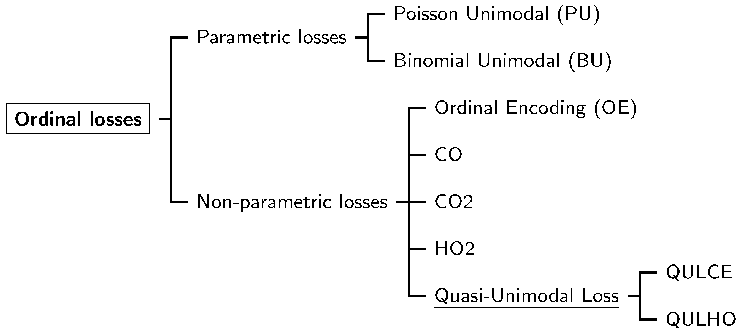
A large body of work in the literature proposes losses that promote a unimodal distribution in class labels . This is often achieved with one of the two main classes of ordinal losses (as illustrated by Figure 1): Parametric losses and non-parametric losses. Parametric losses try to antecedently impose unimodality on the posterior distributions using a single penalty on all the labels.This is done, for example, by assuming that the output function follows a Poisson distribution (PU) [14] or a binomial distribution (BU) [16]. Regarding non-parametric losses, among several in the literature, Ordinal Encoding (OE) [17] or HO2 [2] try not to confine the learned representation to a single parametric model, so that a wider range of possible output functions can be explored, avoiding ad hoc decisions. All the losses mentioned above will be explored in more detail in the next section.
Contributions: For neural networks, a novel non-parametric ordinal loss is presented that induces output probabilities to follow a quasi-unimodal distribution. This is accomplished by applying two different constraints: The first restriction is between the neighboring pair of output probabilities (relative to the true class). Then, a second constrain penalizes all remaining probabilities above that neighborhood, offering a more flexible decision boundary.
2. Related Work
Assume that in a classification task, the instances have one of K classes, whose labels are to , which correspond to the natural order of the ordinal classes.
Cross-Entropy (CE): Typically, a neural network is trained to perform multi-class classification by minimizing the cross-entropy loss for the entire training set,
where, for each n-th observation, , with , representing its respective one-hot encoding and , with being the respective vector of output probabilities assigned by the model for that n-th observation. Naturally, .
However, CE has limitations when applied to ordinal data. Defining as the index of the true class of observation (the position where ), it is then clear that
Intuitively, CE is just trying to maximize the probability in the output corresponding to the true class, ignoring all the other probabilities. For this loss, an error between classes and is treated as the same as an error between and , which is undesirable for ordinal problems.
Furthermore, the loss does not constrain the model to produce unimodal probabilities, so inconsistencies can be produced such as , even when . Cross-entropy is a fair approach for nominal data, where no additional information is available. By concentrating just on the mode of the distribution and disregarding all other values in the output probability vector, the ordinal information inherent in the data is ignored. However, for ordinal data, the order can be explored to further regularize learning.
Ordinal Encoding (OE): Classes are encoded using a cumulative distribution. Therefore, is represented by 1 if and 0 otherwise. Notice that a model should produce class probabilities whose difference should tend to be incremental since it represents a cumulative distribution. This way of introducing ordinality has the advantage of being independent of the way the model is optimized. During inference, to convert back the cumulative distribution to the individual probability of a class k, the differences between classes should be produced , except for the first class [17,18].
Unimodal (U): Constraining the classification output to follow a certain discrete ordinal probability (e.g., binomial or Poisson) may be another approach of promoting ordinality.
- Binomial Unimodal (BU): This directly constrains the neural network’s output, tackling the problem as a regression problem. Instead of several outputs, a single output is predicted, representing the class being predicted. That is, represents and represents [16]. This model has a single output as the final layer which uses a sigmoid activation function to convert it into class probabilities using the binomial probability mass function. This parametric function which is applied to the output probabilities attempts to maintain the ordinality of the classes.
- Poisson Unimodal (PU): Similarly, the constraint for a discrete unimodal probability is enforced by a Poisson probability mass function [14]. On the final layer, the log Poisson probability mass function is applied, followed by a softmax activation function to normalize the output as a probability distribution. According to the authors, it tends to not work as well for more than eight labels [14].
Furthermore, [14] also aims to control the variance of the distribution through a learnable softmax temperature term (). In our experiments, a constant value of was used.
To ensure the ordinality assumption, these parametric techniques may sacrifice accuracy. This tradeoff may be too much in some cases, especially considering the size of the modern deep learning datasets and the high number of mislabeled samples. CE has limitations when applied to ordinal data, as previously stated. By concentrating just on the mode of the distribution and disregarding all other values in the output probability vector, the ordinal information inherent in the data is ignored.
CO and CO2 Ordinal Losses: A regularization term that penalizes deviations from the unimodal setting is added to CE [2].
Defining , a possible fix for an order-aware loss has been previously proposed as
where controls the relative influence of the extra term u which favors unimodal distributions and is defined as
Furthermore, a margin of ensures that the difference between consecutive probabilities is at least [2]. A value of has been empirically found to provide a sensible margin. As a special case, CO has been defined as the case when the margin is zero (),
Ordinal Entropy Loss Function (HO2): Some of the negative aspects of the CE in the CO and CO2 losses have been previously mentioned: It tries to maximize the probability estimated in the true output class while ignoring the remaining probabilities. CO and CO2 promote unimodality, but do not penalize, or barely penalize, flat distributions. A softer assumption is that the distribution should have low entropy [2].
The HO2 tries to tackles these problems by using an entropy term, instead of the cross-entropy term,
where denotes the entropy of the distribution .
3. Proposal
While the HO2 loss mitigates some negative aspects of using CE in the CO and CO2 loss function, it may be too restrictive to penalize probabilities associated with classes that are further from the true class. The motivation for our proposal (quasi-unimodal loss function (QUL)) stems from the definition of the ordinal setting in [19,20], where it is suggested that in a model consistent with the ordinal setting, a small change in the input data should not lead to a “big jump” in the output decision. Assuming as a decision rule that assigns each value of x to the index of the predicted class, the decision rule is said to be consistent with an ordinal data classification setting in a point only if , with representing a neighborhood with a small perturbation (). Equivalently, the decision boundaries in the input space should be only between regions of consecutive classes. Note that the concept of consistency with the ordinal setting is independent of the type of model (probabilistic or not) and relies only on the decision region output by the model.
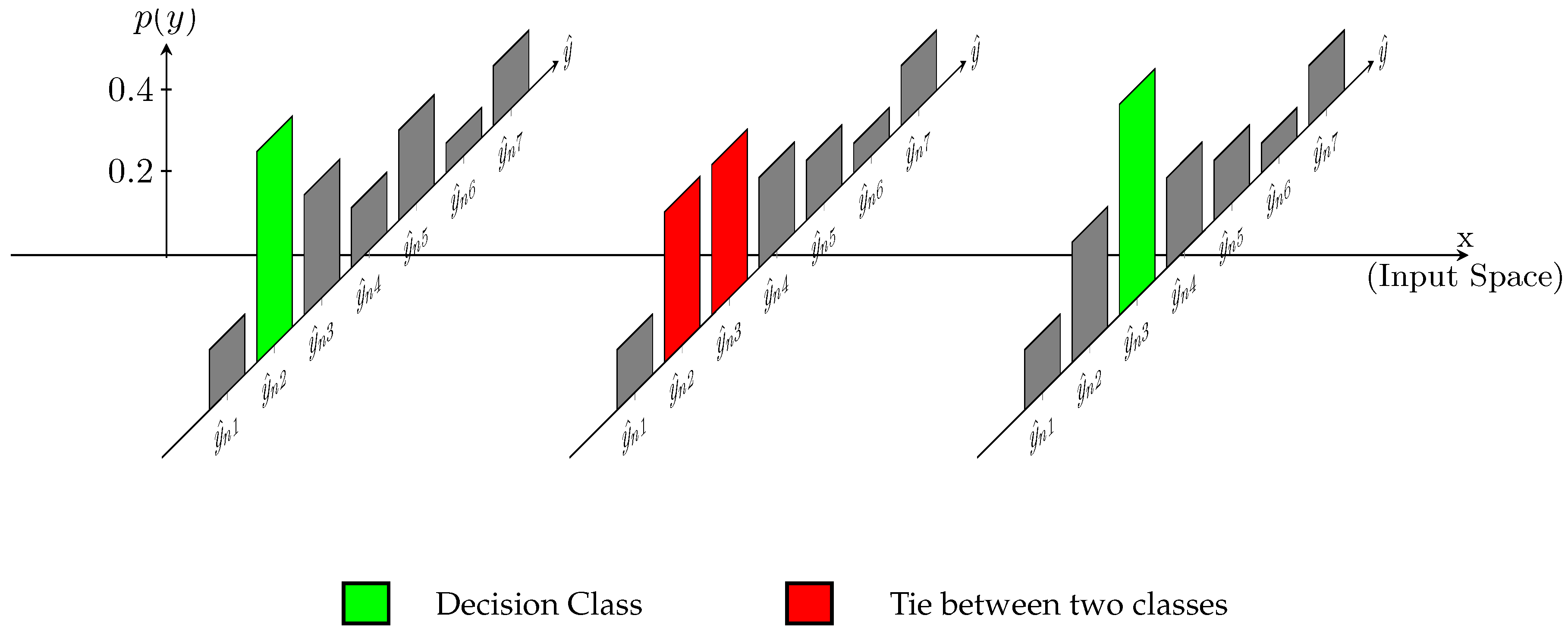
It is easy to conclude that a continuous model that outputs a unimodal distribution in the dimensional probability simplex is ordinal consistent (as long as there are no ties between more than two values in the unimodal distribution). While this is a sufficient condition, unimodality is not necessary to achieve ordinal consistency (Figure 2).
Let be a discrete distribution over the set , with . We say that is a quasi-unimodal distribution (QUD) if:
It should also be clear that a continuous model outputting a QUD in the dimensional probability simplex is ordinal consistent (as long as there are no ties between more than two values in the quasi-unimodal distribution).
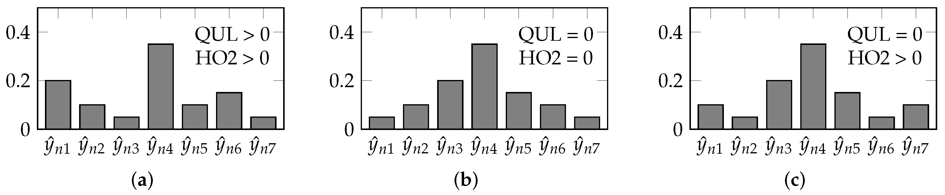
These observations suggest the adoption of a more flexible loss during the training of predictive models, promoting only QUD in the output and not the more restrictive unimodal distribution, as illustrated in Figure 3.
Quasi-unimodal loss function (QUL): Compared to HO2, the ordinal terms in the proposal loss promote unimodality only in the top neighborhood output, which allows for a more flexible curve:
4. Methods
4.1. Architectures
Convolutional neural networks (CNNs) are used since all datasets consist of images. Filters are learnt in these models, which are quadrilateral patches that are convolved throughout the whole input image—unlike fully-connected networks, just a local neighborhood of inputs is coupled at each layer. Each convolution is usually combined with downsampling procedures, such as max-pooling, which gradually lower the size of the original input image while increasing the receptive field.
Three traditional different CNN architectures are used here: MobileNet_V2 [21], ResNet18 [22] and VGG-16 [23]. These three architectures are widely used, well known and frequently referenced in the literature. They were pre-trained on ImageNet using PyTorch (https://pytorch.org/vision/stable/models.html (accessed on: 10 December 2021)).
The following layers were used to replace the last block of each architecture: Dropout with , 512-unit dense layer with ReLU, dropout with , a 256-wide dense layer with ReLU, followed by K output neurons corresponding to the K output classes of each dataset.
4.2. Losses
Eight different losses are evaluated in this work: Cross Entropy (CE) for the baseline model and seven distinct ordinal losses: Ordinal Encoding (OE), Poisson Unimodal (PU), Binomial Unimodal (BU), CO2, Ordinal Entropy Loss Function (HO2), quasi-unimodal entropy loss function (QULHO) and quasi-unimodal cross-entropy loss function (QULCE).
4.3. Training
The weights of the aforementioned architectures were initialized during training using ImageNet pre-training. ADAM was used as the optimizer, with a learning rate of . When the loss is constant for 10 epochs using a specific scheduler, the learning rate is lowered by 10%. The training process is completed after 100 epochs for the Herlev and AFAD dataset; however, the focupath dataset required 300 epochs to finish the training. The training process was conducted on a Nvidia GTX 1080ti (11GB) GPU and on a Nvidia tesla v100 (32 GB). In the case of the ordinal entropy loss function and quasi-unimodal entropy loss function, the hyperparameter is tuned by conducting nested k-fold cross-validating using the training set (with ) to generate an unbiased validation set (∈ [0.00001; 0.0001; 0.001; 0.01; 0.1]). A fix value of was used during the training.
As elaborated in the experimental section below, experiments were also performed in which the loss QULHO was initialized by pre-training on HO2 to further facilitate the optimization process.
5. Experimental Details
5.1. Datasets
Three different datasets are used—Herlev dataset, FocusPath dataset and Asian Face Age Dataset (AFAD)—which will now be elaborated. All these datasets consist of RGB images.
5.1.1. Herlev Dataset
The Herlev dataset collected at the Herlev University Hospital (Denmark) is a publicly accessible dataset (http://mde-lab.aegean.gr/index.php/downloads (accessed on: 5 November 2021)) using a digital camera and microscope with an image resolution of 0.201 m per pixel [24]. The specimens were prepared using the conventional pap smear and pap staining methods. Two cytotechnicians and a doctor classified the cervical images in the Herlev dataset into seven classes to improve the precision of diagnosis.
A total of 917 images of individual cervical cells constitute the Herlev dataset. Each image has a classification label and ground truth segmentation. Table 1 illustrates the nomenclature of the seven different classes from the dataset, wherein classes 1–3 correspond to different types of normal cells and classes 4–7 correspond to varying levels of abnormal cells, according to the World Health Organization (WHO) classification system. Furthermore, The Bethesda System (TBS) classification system condenses the seven classes into only four classes, as illustrated in the table.
5.1.2. FocusPath Dataset
The public histopathological dataset entitled FocusPath (https://zenodo.org/record/3926181#.YPFgluhKjIU (accessed on: 5 November 2021)) contains image quality annotations [25]. The FocusPath dataset contains 8640 patches of 1024 × 1024 images. Nine different stained slides from various human organs were used to create these images. The Huron TissueScope LE1 scanned the original Whole Slide Images. It uses a 40× optics lens at 0.25 resolution. For the focus level, there are 14 absolute z-level scores that correspond to the ground-truth class.
Table 2 shows multiple examples from each of the FocusPath dataset’s classes. Due to the low quantity of examples of images in the more defocused classes (12 and 13), the label was changed to belong to class 11. This way, the dataset was then divided into 12 different focus classes—0 (focus patch) to 11 (defocus patch).
5.1.3. AFAD Dataset
The Asian Face Age Dataset (AFAD) [26] is a publicly available dataset (https://github.com/afad-dataset/tarball (accessed on: 10 November 2021)) used to estimate age. Images smaller than were discarded, resulting in 164,432 photos (63,680 of females and 100,752 of males). The ages range from 15 to 72 for a total of classes (Table 3).
5.2. Data Pre-Processing
The three datasets are partitioned into train, validation, and test subsets (60-20-20%), with the ratio between the different classes maintained. To feed the network and to use the pre-trained architectures on ImageNet it was necessary to resize the images to pixels. As typically done in deep learning models, normalization was also performed to scale the pixel values to 0–1, which speeds up the training process and also helps the network in regularization.
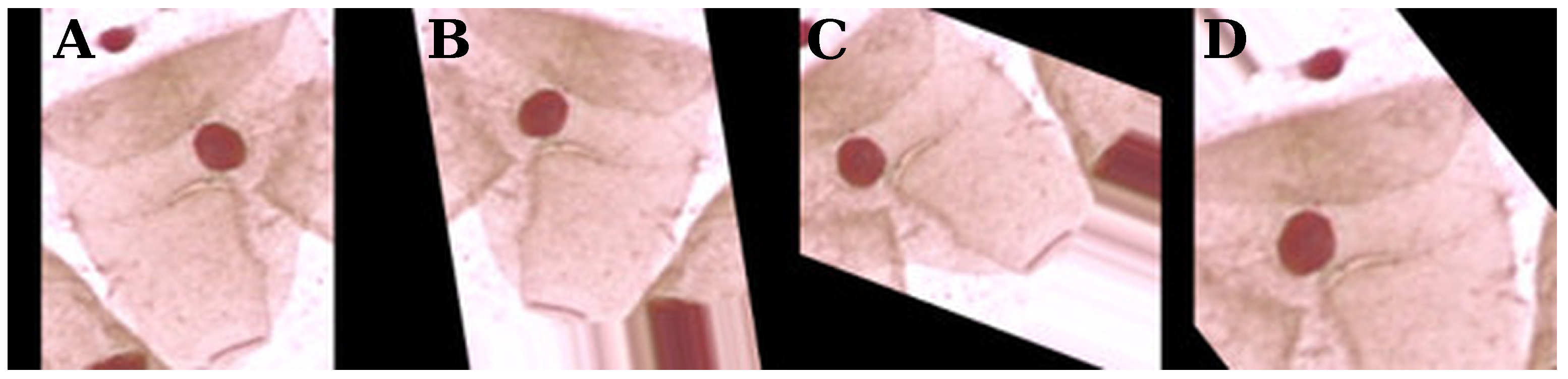
Furthermore, to tackle the small amount of data in the datasets, data augmentation is performed. During training, a series of random transformations are applied to each image: 10% of zoom, 10% of width and height shift, horizontal and vertical flips, and image rotation. These transformations are illustrated in Figure 5.
5.3. Evaluation Metrics
Four distinct metrics were used to assess the performance of the various models: Accuracy, mean absolute error (MAE), mean squared error (MSE), and the Uniform Ordinal Classification Index (UOC).
Accuracy (ACC) is one of the most commonly used measures in classification tasks. For N observations, taking and to be the label and prediction of the n-th observation, respectively, then where is the indicator function.
However, this metric treats all class errors as equal, whether the error is between adjacent classes or between classes in the extreme. If we have K classes represented by a set , then accuracy will treat an error between and with the same magnitude as an error between and which is clearly worse. For that reason, a popular metric for ordinal classification is the Mean Absolute Error (MAE), This metric is not perfect since it treats an ordinal variable as a cardinal variable. An error between classes and will be treated as two times worse than an error between classes and . Naturally, the assumption of cardinality is not always warranted. In Mean Squared Error (MSE), instead of being the absolute difference as in MAE, the squared difference is computed between the output of the classifier and the correct label over all examples. This makes the error more pronounced the further away the predicted class is to the true class [27].
Uniform ordinal classification index (UOC) is a recent metric which combines accuracy and ranking in performance assessment and is also robust against imbalanced classes [28]. The better the performance, the lower the UOC. UOC consists of a minimization over the set of all consistent paths that can be traced over the confusion matrix, similar to ordinal classification index (OC) [29]. Each path has a benefit and a penalty, with the benefit being for paths that better follow the natural order of the classes and the penalty being for paths that deviate from the main diagonal, incorporating a classification component into the performance evaluation. Unlike OC, UOC is based on a probabilistic approach, with class priors replaced by a uniform class distribution, making it robust to class imbalance.
By combining these four different evaluation metrics we hope to provide a balanced view of the performance of the methods.
6. Results and Discussion
The models’ performances for the 10-fold (Herlev and FocusPath datasets) and 1-fold (AFAD dataset) using three distinct architectures and three different datasets are presented in Table 4, Table 5, Table 6 and Table 7, with the eight different learning losses—conventional Cross-Entropy (CE), Binomial Unimodal (BU) [16], Poisson Unimodal (PU) [14], Ordinal Encoding (OE) [18], CO2, Ordinal Entropy Loss (HO2) [2], and our proposal losses QULCE and QULHO as measured by MAE, accuracy, MSE and UOC as detailed in the previous section. The best models are shown in bold.
In general, results are fairly close—except that the proposed losses sometimes having a high variance due to them being harder to optimize. For that reason, we introduce a version that is pre-trained from the HO2 loss, in order to mitigate such optimization problems.
Even so, the proposed loss is quite competitive, especially on the Herlev dataset. Please notice that BU and PU fail to run as the number of classes increases after a certain point.
In the results for the AFAD dataset, due to a large number of classes, HO2 and QULHO losses have optimization problems, which suggests that a more exhaustive fine-tuning of hyper-parameters must be done.
The present work intends to promote the use of ordinal losses against nominal losses when the problem at hand has ordinal data. In the Herlev and FocusPath dataset in most of the cases ordinal losses, across the four different metrics, had better results than nominal cross-entropy loss.
7. Conclusions
In ordinal classification, metrics are most concerned about the relative order of the predictions, rather than the absolute order. That is, an error between two distant classes is deemed worse than an error between two neighboring classes. For that reason, a wide variety of losses can be found in the literature.
In this work, a novel non-parametric ordinal loss is proposed, which induces output probabilities to follow a quasi-unimodal distribution. Other strategies in the literature involve large modifications in architecture or data format; therefore, the suggested loss is a handy way to introduce ordinality in the classification task without requiring substantial changes in design or data format. It improves upon previous work by allowing for a more flexible distribution since the unimodal constraint is relaxed for other classes outside the top-three neighborhood. Furthermore, a review of existing ordinal losses is provided.
Several losses from the literature, plus the proposed one, are compared in an empirical assessment which comprises three different datasets using three popular neural network architectures. The parametric losses that were evaluated fail after the number of classes are increased beyond a certain point. The proposed loss seems competitive in terms of scalability and consistency.
Author Contributions
Conceptualization, T.A., R.C. and J.S.C.; methodology, T.A., R.C. and J.S.C.; validation, T.A., R.C.; formal analysis, T.A., R.C. and J.S.C.; investigation, T.A., R.C. and J.S.C.; writing—original draft preparation, T.A., R.C. and J.S.C.; writing—review and editing, T.A., R.C. and J.S.C.; visualization, T.A., R.C. and J.S.C.; supervision, J.S.C.; project administration, J.S.C.; funding acquisition, J.S.C. All authors have read and agreed to the published version of the manuscript.
Funding
The project TAMI-Transparent Artificial Medical Intelligence (NORTE-01-0247-FEDER-045905) partially funding this work is co-financed by ERDF - European Regional Fund through the North Portugal Regional Operational Program-NORTE 2020 and by the Portuguese Foundation for Science and Technology-FCT under the CMU-Portugal International Partnership. Tomé Albuquerque was supported by Ph.D. grant 2021.05102.BD, also provided by FCT.
Institutional Review Board Statement
Not applicable.
Informed Consent Statement
Not applicable.
Data Availability Statement
All the datasets used in this work are publicly available: Herlev dataset—http://mde-lab.aegean.gr/index.php/downloads (accessed on: 5 November 2021); FocusPath dataset—https://zenodo.org/record/3926181#.YPFgluhKjIU (accessed on: 5 November 2021); AFAD dataset—https://github.com/afad-dataset/tarball (accessed on: 10 November 2021).
Acknowledgments
The authors would like to acknowledge access to the Herlev Pap smear dataset collected by Herlev University Hospital (Denmark) and the Technical University of Denmark.
Conflicts of Interest
The authors declare no conflict of interest.
Abbreviations
The following abbreviations are used in this manuscript:
| ACC | Accuracy |
| BU | Binomial Unimodal |
| CE | Cross-entropy |
| CNN | Convolutional Neural Network |
| MAE | Mean Average Precision |
| MSE | Mean Squared Error |
| OE | Ordinal Encoding |
| PU | Poisson Unimodal |
| QUL | Quasi-unimodal loss function |
| QULHO | Quasi-unimodal entropy loss function |
| QULCE | Quasi-unimodal cross-entropy loss function |
| TBS | The Bethesda System |
| WHO | World Health Organization |
References
- Belharbi, S.; Ayed, I.B.; McCaffrey, L.; Granger, E. Non-parametric Uni-modality Constraints for Deep Ordinal Classification. arXiv 2020, arXiv:1911.10720. [Google Scholar]
- Albuquerque, T.; Cruz, R.; Cardoso, J.S. Ordinal losses for classification of cervical cancer risk. PeerJ Comput. Sci. 2021, 7, e457. [Google Scholar] [CrossRef] [PubMed]
- Liu, H.; Lu, J.; Feng, J.; Zhou, J. Ordinal Deep Feature Learning for Facial Age Estimation. In Proceedings of the 2017 12th IEEE International Conference on Automatic Face Gesture Recognition (FG 2017), Washington, DC, USA, 30 May–3 June 2017; pp. 157–164. [Google Scholar] [CrossRef]
- Pan, H.; Han, H.; Shan, S.; Chen, X. Mean-Variance Loss for Deep Age Estimation from a Face. In Proceedings of the 2018 IEEE/CVF Conference on Computer Vision and Pattern Recognition, Salt Lake City, UT, USA, 18–23 June 2018; pp. 5285–5294. [Google Scholar] [CrossRef]
- Zhu, H.; Zhang, Y.; Li, G.; Zhang, J.; Shan, H. Ordinal Distribution Regression for Gait-based Age Estimation. Sci. China Inf. Sci. 2020, 63, 120102. [Google Scholar] [CrossRef] [Green Version]
- Crammer, K.; Singer, Y. Pranking with Ranking. In Advances in Neural Information Processing Systems; Dietterich, T., Becker, S., Ghahramani, Z., Eds.; MIT Press: Cambridge, MA, USA, 2002; Volume 14. [Google Scholar]
- Koren, Y.; Sill, J. OrdRec: An ordinal model for predicting personalized item rating distributions. In Proceedings of the Fifth ACM Conference on Recommender Systems, Chicago, IL, USA, 23–27 October 2011; pp. 117–124. [Google Scholar] [CrossRef]
- Gentry, A.; Jackson-Cook, C.; Lyon, D.; Archer, K. Penalized Ordinal Regression Methods for Predicting Stage of Cancer in High-Dimensional Covariate Spaces. Cancer Inform. 2015, 14, 201–208. [Google Scholar] [CrossRef] [PubMed] [Green Version]
- Moody, J.E.; Utans, J. Architecture Selection Strategies for Neural Networks: Application to Corporate Bond Rating Predicti. In Proceedings of the Neural Networks in the Capital Markets, NIPS 1995, Denver, CO, USA, 27 November–2 December 1995. [Google Scholar]
- Jia, X.; Zheng, X.; Li, W.; Zhang, C.; Li, Z. Facial Emotion Distribution Learning by Exploiting Low-Rank Label Correlations Locally. In Proceedings of the 2019 IEEE/CVF Conference on Computer Vision and Pattern Recognition (CVPR), Long Beach, CA, USA, 15–20 June 2019; pp. 9833–9842. [Google Scholar] [CrossRef]
- Xiong, H.; Liu, H.; Zhong, B.; Fu, Y. Structured and Sparse Annotations for Image Emotion Distribution Learning. Proc. AAAI Conf. Artif. Intell. 2019, 33, 363–370. [Google Scholar] [CrossRef]
- Zhou, Y.; Xue, H.; Geng, X. Emotion Distribution Recognition from Facial Expressions. In Proceedings of the MM ’15: Proceedings of the 23rd ACM International Conference on Multimedia, New York, NY, USA, 26–30 October 2015; Association for Computing Machinery: New York, NY, USA, 2015; pp. 1247–1250. [Google Scholar] [CrossRef]
- Palermo, F.; Hays, J.; Efros, A. Dating Historical Color Images. In European Conference on Computer Vision; Springer: Heidelberg, Germany, 2012; Volume 7577, pp. 499–512. [Google Scholar] [CrossRef] [Green Version]
- Beckham, C.; Pal, C. Unimodal Probability Distributions for Deep Ordinal Classification. In Proceedings of the 34th International Conference on Machine Learning, Sydney, Australia, 6–11 August 2017; Precup, D., Teh, Y.W., Eds.; PMLR: Sydney, Australia, 2017; Volume 70, pp. 411–419. [Google Scholar]
- Cardoso, J.S.; Pinto da Costa, J.F. Learning to Classify Ordinal Data: The Data Replication Method. J. Mach. Learn. Res. 2007, 8, 1393–1429. [Google Scholar]
- Costa, J.; Cardoso, J. Classification of Ordinal Data Using Neural Networks. In European Conference on Machine Learning; Springer: Berlin/Heidelberg, Germany, 2005; pp. 690–697. [Google Scholar] [CrossRef] [Green Version]
- Frank, E.; Hall, M. A simple approach to ordinal classification. In European Conference on Machine Learning; Springer: Berlin/Heidelberg, Germany, 2001; pp. 145–156. [Google Scholar] [CrossRef] [Green Version]
- Cheng, J.; Wang, Z.; Pollastri, G. A neural network approach to ordinal regression. In Proceedings of the 2008 IEEE International Joint Conference on Neural Networks (IEEE World Congress on Computational Intelligence), Hong Kong, China, 1–8 June 2008; pp. 1279–1284. [Google Scholar]
- Cardoso, J.S.; Sousa, R. Classification Models with Global Constraints for Ordinal Data. In Proceedings of the 2010 Ninth International Conference on Machine Learning and Applications, Washington, DC, USA, 12–14 December 2010; pp. 71–77. [Google Scholar] [CrossRef]
- Sousa, R.; Cardoso, J.S. Ensemble of decision trees with global constraints for ordinal classification. In Proceedings of the 2011 11th International Conference on Intelligent Systems Design and Applications, Córdoba, Spain, 22–24 November 2011; pp. 1164–1169. [Google Scholar] [CrossRef] [Green Version]
- Howard, A.G.; Zhu, M.; Chen, B.; Kalenichenko, D.; Wang, W.; Weyand, T.; Andreetto, M.; Adam, H. MobileNets: Efficient convolutional neural networks for mobile vision applications. arXiv 2017, arXiv:1704.04861. [Google Scholar]
- He, K.; Zhang, X.; Ren, S.; Sun, J. Deep residual learning for image recognition. In Proceedings of the IEEE Conference on Computer Vision and Pattern Recognition, Las Vegas, NV, USA, 27–30 June 2016; pp. 770–778. [Google Scholar]
- Simonyan, K.; Zisserman, A. Very deep convolutional networks for large-scale image recognition. arXiv 2014, arXiv:1409.1556. [Google Scholar]
- Jantzen, J.; Dounias, G. Analysis of Pap-smear image data. In Proceedings of the Nature-Inspired Smart Information Systems 2nd Annual Symposium, Austria, 29 November–1 December 2006; Volume 10. [Google Scholar]
- Hosseini, M.S.; Zhang, Y.; Plataniotis, K.N. Encoding Visual Sensitivity by MaxPol Convolution Filters for Image Sharpness Assessment. IEEE Trans. Image Process. 2019, 28, 4510–4525. [Google Scholar] [CrossRef] [Green Version]
- Niu, Z.; Zhou, M.; Wang, L.; Gao, X.; Hua, G. Ordinal Regression With Multiple Output CNN for Age Estimation. In Proceedings of the IEEE Conference on Computer Vision and Pattern Recognition (CVPR), Las Vegas, NV, USA, 27–30 June 2016. [Google Scholar]
- Gaudette, L.; Japkowicz, N. Evaluation Methods for Ordinal Classification. In Advances in Artificial Intelligence; Gao, Y., Japkowicz, N., Eds.; Springer: Berlin/Heidelberg, Germany, 2009; pp. 207–210. [Google Scholar]
- Silva, W.; Pinto, J.R.; Cardoso, J.S. A Uniform Performance Index for Ordinal Classification with Imbalanced Classes. In Proceedings of the 2018 International Joint Conference on Neural Networks (IJCNN), Rio de Janeiro, Brazil, 8–13 July 2018; pp. 1–8. [Google Scholar]
- Cardoso, J.; Sousa, R. Measuring the Performance of Ordinal Classification. Int. J. Pattern Recognit. Artif. Intell. 2011, 25, 1173–1195. [Google Scholar] [CrossRef] [Green Version]
Figure 1.
Schematic representation of ordinal loss functions from the literature. The proposed loss function is underlined.
Figure 1.
Schematic representation of ordinal loss functions from the literature. The proposed loss function is underlined.

Figure 2.
Schematic representation of an example where there is ordinal consistency in the decision, without a unimodal distribution in the classes. X axis corresponds to the input space (x) of the model, and Y axis corresponds to output probabilities () of the model. Along x, an example of a decision region is represented where the model chooses between two different classes with a boundary region between this decision.

Figure 3.
Probabilities produced by three different models for an observation n. HO2 forces the entire distribution curve to have decreasing probabilities. On the other hand, QULHO focuses on the top neighborhood, and is not as concerned about the more distant classes. In this example, is assumed to be the true class. (a) Non-unimodal; (b) Unimodal; (c) Quasi-unimodal.

Figure 4.
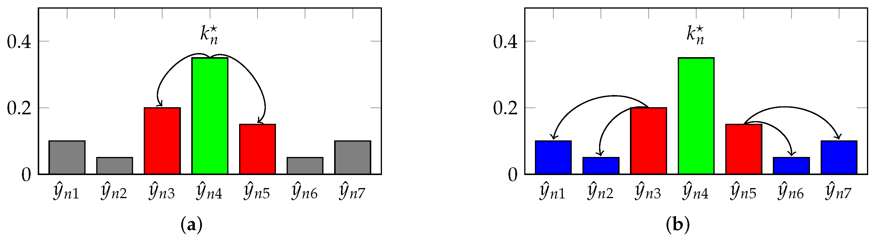
Schematic representation of the two QUL terms as in Equation (9): The first term penalizes only the direct neighborhood, while the second term penalizes the remaining classes relative to the neighborhood. (a) First QUL term; (b) Second QUL term.
Figure 4.
Schematic representation of the two QUL terms as in Equation (9): The first term penalizes only the direct neighborhood, while the second term penalizes the remaining classes relative to the neighborhood. (a) First QUL term; (b) Second QUL term.

Figure 5.
Examples of data augmentation on the Herlev database. The original zero-padding image (A) and random transformations (B–D).
Figure 5.
Examples of data augmentation on the Herlev database. The original zero-padding image (A) and random transformations (B–D).


Table 1.
Illustration with images of the seven different classes in the Herlev dataset.
| Normal | Abnormal | ||||||
|---|---|---|---|---|---|---|---|
 |  |  |  |  |  |  | |
| WHO | |||||||
| TBS | |||||||
Table 2.
Examples of 14 FocusPath classes.
 |  |  |  |  |  |  |  |  |  |  |  |  |  |
|---|---|---|---|---|---|---|---|---|---|---|---|---|---|
 |  |  |  |  |  |  |  |  |  |  |  |  |  |
 |  |  |  |  |  |  |  |  |  |  |  |  |  |
| 0 | 1 | 2 | 3 | 4 | 5 | 6 | 7 | 8 | 9 | 10 | 11 | 12 | 13 |
| Focus Level—focus(0) → defocus(13) | |||||||||||||
Table 3.
Examples of six different classes from the AFAD dataset.
 |  |  |  |  |  |
|---|---|---|---|---|---|
 |  |  |  |  |  |
| 15 | 25 | 35 | 45 | 55 | 66 |
| Age (− → +) | |||||
Table 4.
Results for the Herlev dataset when considering seven classes, averaged for 10 folds.
| Mean Absolute Error (MAE) | Accuracy (%) | |||||||
| MobileNet_v2 | ResNet18 | VGG16 | Avg | MobileNet_v2 | ResNet18 | VGG16 | Avg | |
| CE | 0.37 | 73.4 | ||||||
| BU | 0.41 | 66.2 | ||||||
| PU | 0.39 | 70.1 | ||||||
| OE | 0.36 | 72.8 | ||||||
| CO2 | 0.37 | 72.6 | ||||||
| HO2 | 0.37 | 72.0 | ||||||
| QULCE | 0.35 | 74.2 | ||||||
| QULHO | 0.33 | 73.6 | ||||||
| Mean Squared Error (MSE) | UOC (%) | |||||||
| MobileNet_v2 | ResNet18 | VGG16 | Avg | MobileNet_v2 | ResNet18 | VGG16 | Avg | |
| CE | 0.60 | 36.9 | ||||||
| BU | 0.53 | 42.3 | ||||||
| PU | 0.58 | 38.8 | ||||||
| OE | 0.56 | 37.2 | ||||||
| CO2 | 0.55 | 37.9 | ||||||
| HO2 | 0.55 | 37.9 | ||||||
| QULCE | 0.60 | 37.3 | ||||||
| QULHO | 0.51 | 36.7 | ||||||
bold: best model.
Table 5.
Results for the Herlev dataset when considering four classes, averaged for 10 folds.
| Mean Absolute Error (MAE) | Accuracy (%) | |||||||
| MobileNet_v2 | ResNet18 | VGG16 | Avg | MobileNet_v2 | ResNet18 | VGG16 | Avg | |
| CE | 0.25 | 79.2 | ||||||
| BU | 0.27 | 76.5 | ||||||
| PU | 0.25 | 77.8 | ||||||
| OE | 0.24 | 79.2 | ||||||
| CO2 | 0.25 | 78.5 | ||||||
| HO2 | 0.26 | 77.8 | ||||||
| QULCE | 0.25 | 78.9 | ||||||
| QULHO | 0.25 | 79.2 | ||||||
| Mean Squared Error (MSE) | UOC (%) | |||||||
| MobileNet_v2 | ResNet18 | VGG16 | Avg | MobileNet_v2 | ResNet18 | VGG16 | Avg | |
| CE | 0.34 | 32.2 | ||||||
| BU | 0.31 | 32.8 | ||||||
| PU | 0.31 | 33.2 | ||||||
| OE | 0.29 | 30.8 | ||||||
| CO2 | 0.31 | 32.5 | ||||||
| HO2 | 0.33 | 32.9 | ||||||
| QULCE | 0.35 | 33.0 | ||||||
| QULHO | 0.33 | 32.6 | ||||||
bold: best model.
Table 6.
Results for the FocusPath dataset, averaged for 10 folds.
| Mean Absolute Error (MAE) | Accuracy (%) | |||||||
| MobileNet_v2 | ResNet18 | VGG16 | Avg | MobileNet_v2 | ResNet18 | VGG16 | Avg | |
| CE | 0.12 | 88.6 | ||||||
| PU | − | − | − | − | − | − | − | − |
| BU | 0.29 | 79.4 | ||||||
| OE | 0.11 | 89.2 | ||||||
| CO2 | 0.14 | 86.6 | ||||||
| HO2 | 0.16 | 85.3 | ||||||
| QULCE | 0.16 | 85.6 | ||||||
| QULHO | 0.15 | 86.3 | ||||||
| Mean Squared Error (MSE) | UOC (%) | |||||||
| MobileNet_v2 | ResNet18 | VGG16 | Avg | MobileNet_v2 | ResNet18 | VGG16 | Avg | |
| CE | 0.17 | 22.0 | ||||||
| BU | 0.20 | 29.4 | ||||||
| PU | 9.83 | 52.7 | ||||||
| OE | 0.12 | 21.4 | ||||||
| CO2 | 0.17 | 26.2 | ||||||
| HO2 | 0.21 | 30.4 | ||||||
| QULCE | 2.09 | 54.6 | ||||||
| QULHO | 0.18 | 27.8 | ||||||
bold: best model.
Table 7.
Results for the AFAD dataset, averaged for three folds.
| Mean Absolute Error (MAE) | Accuracy (%) | |||||||
| MobileNet_v2 | ResNet18 | VGG16 | Avg | MobileNet_v2 | ResNet18 | VGG16 | Avg | |
| CE | 0.02 | 99.5 | ||||||
| PU | − | − | − | − | − | − | − | − |
| BU | − | − | − | − | − | − | − | − |
| OE | 0.03 | 98.0 | ||||||
| CO2 | 0.27 | 92.0 | ||||||
| HO2 | 2.61 | 58.4 | ||||||
| QULCE | 0.07 | 98.5 | ||||||
| QULHO | 2.51 | 62.3 | ||||||
| Mean Squared Error (MSE) | UOC (%) | |||||||
| MobileNet_v2 | ResNet18 | VGG16 | Avg | MobileNet_v2 | ResNet18 | VGG16 | Avg | |
| CE | 0.09 | 1.8 | ||||||
| PU | − | − | − | − | − | − | − | − |
| BU | − | − | − | − | − | − | − | − |
| OE | 0.09 | 19.3 | ||||||
| CO2 | 2.87 | 79.7 | ||||||
| HO2 | 26.66 | 98.9 | ||||||
| QULCE | 0.62 | 10.3 | ||||||
| QULHO | 25.95 | 98.8 | ||||||
bold: best model.
Publisher’s Note: MDPI stays neutral with regard to jurisdictional claims in published maps and institutional affiliations. |
© 2022 by the authors. Licensee MDPI, Basel, Switzerland. This article is an open access article distributed under the terms and conditions of the Creative Commons Attribution (CC BY) license (https://creativecommons.org/licenses/by/4.0/).
Share and Cite
MDPI and ACS Style
Albuquerque, T.; Cruz, R.; Cardoso, J.S. Quasi-Unimodal Distributions for Ordinal Classification. Mathematics 2022, 10, 980. https://0-doi-org.brum.beds.ac.uk/10.3390/math10060980
AMA Style
Albuquerque T, Cruz R, Cardoso JS. Quasi-Unimodal Distributions for Ordinal Classification. Mathematics. 2022; 10(6):980. https://0-doi-org.brum.beds.ac.uk/10.3390/math10060980
Chicago/Turabian StyleAlbuquerque, Tomé, Ricardo Cruz, and Jaime S. Cardoso. 2022. "Quasi-Unimodal Distributions for Ordinal Classification" Mathematics 10, no. 6: 980. https://0-doi-org.brum.beds.ac.uk/10.3390/math10060980
Note that from the first issue of 2016, this journal uses article numbers instead of page numbers. See further details here.