Jointly Modeling Rating Responses and Times with Fuzzy Numbers: An Application to Psychometric Data

Abstract

In several research areas, ratings data and response times have been successfully used to unfold the stagewise process through which human raters provide their responses to questionnaires and social surveys. A limitation of the standard approach to analyze this type of data is that it requires the use of independent statistical models. Although this provides an effective way to simplify the data analysis, it could potentially involve difficulties with regard to statistical inference and interpretation. In this sense, a joint analysis could be more effective. In this research article, we describe a way to jointly analyze ratings and response times by means of fuzzy numbers. A probabilistic tree model framework has been adopted to fuzzify ratings data and four-parameters triangular fuzzy numbers have been used in order to integrate crisp responses and times. Finally, a real case study on psychometric data is discussed in order to illustrate the proposed methodology. Overall, we provide initial findings to the problem of using fuzzy numbers as abstract models for representing ratings data with additional information (i.e., response times). The results indicate that using fuzzy numbers leads to theoretically sound and more parsimonious data analysis methods, which limit some statistical issues that may occur with standard data analysis procedures.

1. Introduction

Rating scales and questionnaires are widespread in behavioral and social sciences and are especially useful in collecting human opinions, attitudes, and socio-demographic information. A typical rating task entails a multicomponential sequence of cognitive tasks which drive raters to provide their response by selecting one of the possible response categories [1]. It is well-accepted that mining the raters’ response process can provide new insights into the mechanisms underlying rating choices [2,3]. To this end, fuzzy set theory has been widely applied in modeling the non-random and subjective components of the rating response (for a recent review, see [4]). By and large, two general approaches can be recognized in the fuzzy rating literature, namely fuzzy direct scales and fuzzy conversion scales. While the former asks raters to provide their response by means of a stage-wise methodology, which is in turn supposed to elicit the subjective components of the rating response (e.g., see [5,6,7]), the latter aims at turning standard rating data into fuzzy numbers by means of expert-based or statistical-based procedures (e.g., see [8,9,10]). Despite the differences on the way of mapping fuzzy numbers to the rating process, both provide a valuable strategy to avoid the loss of subjective information entailed by standard rating response formats [11,12].

Recently, a novel fuzzy conversion procedure (fIRTree) has been proposed with the aim of quantifying a particular component of the rating process, namely the rater’s decision uncertainty [13,14]. The fIRTree procedure is based upon the use of the Item Response Theory-based trees (IRTree), which model the stage-wise rating processes in terms of linear or nested statistical trees [15]. In particular, once an IRTree model has been fit to crisp rating data, fIRTree uses the estimated IRT parameters to map parametric fuzzy numbers to crisp ratings data. In addition, when the four-parameter triangular fuzzy numbers are used [16], fIRTree allows for integrating rating responses and response times into a unique parametric representation. In doing so, fIRTree provides a more flexible and parsimonious representation of uncertainty in ratings data.

In this paper, we describe how parametric fuzzy numbers can be easily used to integrate multiple sources of rating information, such as rating responses and response times. The aim is twofold. First, we show how the four-parameter triangular fuzzy numbers [16] can be used to jointly model fIRTree-based raters’ responses and time in a unique formal representation [13]. The importance of response times in quantifying characteristics of the rating process (e.g., item/question’s difficulty) has been widely established in the psychometric literature [17]. Second, we describe a way to analyze and make inference on this type of data by means of an integrated fuzzy statistical framework. To this end, we adopt an epistemic-based fuzzy normal linear model with crisp predictors, where the problem of point estimation for the unknown parameters is addressed using the minimum inaccuracy principle [18]. Fuzzy regression models are widespread methods to analyze fuzzy data [19,20,21]. According to the epistemic interpretation of a fuzzy set [22], fuzzy data are affected by two types of imprecision: stochastic imprecision–which is related to the probabilistic model underlying the observations—and possibilistic imprecision—which is in turn associated with an incomplete knowledge of the originally crisp observations [23,24]. Finally, a real case study based on psychometric data is used in order to highlight the features of the proposed approach with regards to more traditional data analysis procedures.

The remainder of this paper is structured as follows. Section 2 presents an overview of fuzzy numbers, fIRTree models, and the fuzzy normal linear model with crisp predictors. Section 3 illustrates an application of the new methodology on clinical questionnaire data along with a comparison with standard data analyses. Finally, Section 4 provides final remarks on the current findings.

2. Methodology

2.1. Fuzzy Numbers

A fuzzy subset $\tilde{A}$ of a universal set $\mathcal{A}$ is defined by its membership function ${\xi }_{\tilde{A}}:\mathcal{A}\to [0,1]$. It can be described as a collection of crisp subsets called $\alpha$-sets, i.e., ${\tilde{A}}_{\alpha }=\{y\in \mathcal{A}:{\xi }_{\tilde{A}}(y)>\alpha \}$ with $\alpha \in (0,1]$. If the $\alpha$-sets of $\tilde{A}$ are all convex sets, then $\tilde{A}$ is a convex fuzzy set. The support of $\tilde{A}$ is $A_0=\{y\in \mathcal{A}:{\xi }_{\tilde{A}}(y)>0\}$ and the core is the set of all its maximal points $A_c=\{y\in \mathcal{A}:{\xi }_{\tilde{A}}(y)={max}_{y\in \mathcal{A}}{\xi }_{\tilde{A}}(y)\}$. In the case where ${max}_{y\in \mathcal{A}}{\xi }_{\tilde{A}}(y)=1$, then $\tilde{A}$ is a normal fuzzy set. If $\tilde{A}$ is a normal and convex subset of $\mathbb{R}$, then $\tilde{A}$ is a fuzzy number. The class of all normal fuzzy numbers is denoted by $\mathcal{F}(\mathbb{R})$. Fuzzy numbers can be represented using parametric models that are indexed by some scalars, such as c (mode) and s (spread or precision). A particular type of parametric fuzzy number is the so-called four-parameters triangular fuzzy number [16]:

$${\xi }_{\tilde{A}}(y;c,l,r,\omega )={\left(1+{\left(\frac{c-y}{y-l}\right)}^{\omega }\right)}^{-1}·{\mathbb{𝟙}}_{[l,c]}(y)+{\left(1+{\left(\frac{r-y}{y-c}\right)}^{-\omega }\right)}^{-1}·{\mathbb{𝟙}}_{(c,r]}(y)$$

(1)

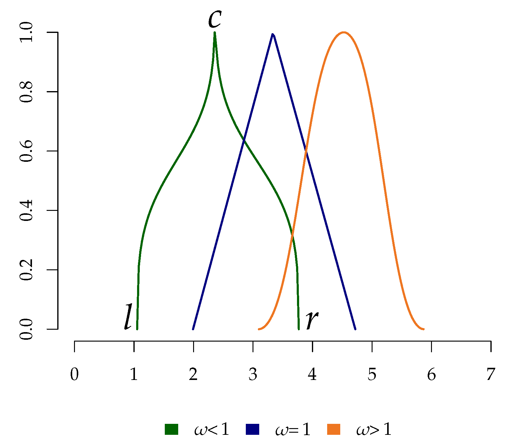
where $-\infty <l<c<r<+\infty$ and $\omega \in {\mathbb{R}}_0^{+}$. The fuzziness of the set is controlled by the parameter $\omega$, which provides an intensification ($\omega <1$) or a reduction ($\omega >1$) of its shape. The versatility of such a fuzzy number offers a way to integrate different sources of uncertainty into a unique formal representation. Note that the parameter $\omega$ allows for increasing or decreasing the overall fuzziness of the set [25]. Moreover, four-parameter fuzzy numbers require just one intensification parameter (e.g., differently from [26]), providing a balance between flexibility and complexity. According to the inverted-U effect between response times and responses on Likert scales, raters tend to show longer response times especially with middle-scale responses [27,28]. In this context, $\omega$ can be modulated so that longer response times—which are usually provided by raters who are very hesitant about their final choices—produce an intensification of the fuzziness whereas shorter response times—that are usually provided by raters who are quite sure about their final choices–produce a reduction of the fuzziness. As a result, the fuzziness of the set can be interpreted as a proxy for the rater’s decision uncertainty. Figure 1 shows an example of the relationship between fuzziness and the $\omega$ parameter.

2.2. From IRTree to fIRTree

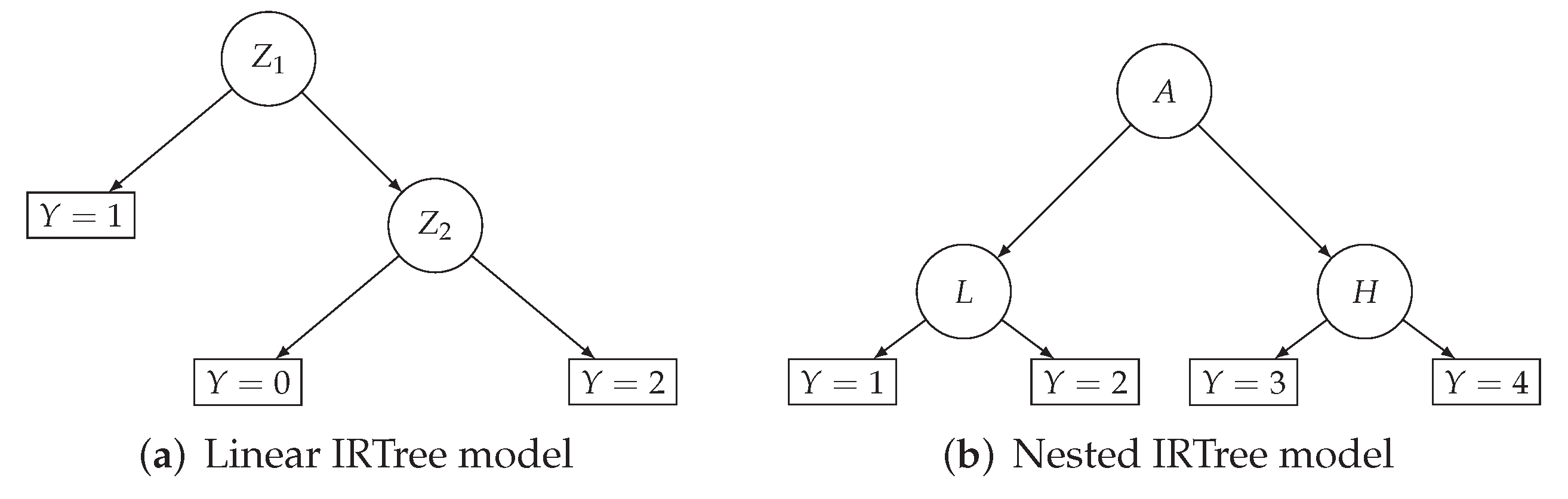
Item Response Theory (IRT) trees are conditional linear models that represent ratings data in terms of binary trees. In general, the tree formalizes the rating response process as a sequence of intermediate nodes, each of which corresponds to a cognitive decision, and end-nodes, which codify the possible final choices or answers. Figure 2 depicts two examples of IRTree models for a rating scale with three and four response categories. In particular, the first tree (Figure 2a) formalizes a typical situation where the rater first decides whether he/she is neutral about the item/question being assessed ($Z_1$) and then he/she decides about the strength of the agreement or disagreement ($Z_2$). As a byproduct of the binary structure, the probability of a final response (e.g., $Y=1$: Neutral) can be computed by multiplying the probabilities of each branch (e.g., $P(Y=1)=P(Z_1=0;\mathit{\theta })$).

By adopting the IRT parametrization, the parameter array $\mathit{\theta }$ can be defined as to contain rater-specific and item-specific parameters. Thus, the probability to agree or disagree with an item/question can be represented as a function of a rater’s latent trait and the specific content of the item [15]. More formally, let $i\in \{1,\dots ,I\}$ and $j\in \{1,\dots ,J\}$ be the indices for raters and items, respectively. Then, the final response variable $Y_{ij}\in \{1,\dots ,m,\dots ,M\}\subset \mathbb{N}$ (M is the maximum number of response categories) can be written as a function of N binary variables $Z_{ijn}\in \{0,1\}$, with $n\in \{1,\dots ,N\}$ denoting the nodes of the tree. For instance, in Figure 2a, the final response $Y_{ij}=0$ corresponds to $Z_{ij2}=0$. For a generic pair $(i,j)$ of data, the IRTree model consists of the following equations:

$$\begin{array}{cc}\hfill & {\mathit{\eta }}_i\sim N_N(\mathbf{0},{\mathbf{\Sigma }}_{\eta }),\hfill \end{array}$$

(2)

$$\begin{array}{cc}\hfill & {\pi }_{ijn}=\mathbb{P}(Z_{ijn}=1;{\mathit{\theta }}_n)=\frac{exp\left({\eta }_{in}+{\alpha }_{jn}\right)}{1+exp\left({\eta }_{in}+{\alpha }_{jn}\right)},\hfill \end{array}$$

(3)

$$\begin{array}{cc}\hfill & Z_{ijn}\sim Ber({\pi }_{ijn}),\hfill \end{array}$$

(4)

where ${\mathit{\theta }}_n=\{{\mathit{\alpha }}_j,{\mathit{\beta }}_i\}$, with the arrays ${\mathit{\alpha }}_j\in {\mathbb{R}}^N$ and ${\mathit{\eta }}_i\in {\mathbb{R}}^N$ denoting the easiness of the item and the rater’s latent trait. As is usual in IRT models, latent traits for each node are modeled using a N-variate centered Gaussian distribution with covariance matrix ${\mathbf{\Sigma }}_{\eta }$. In this representation, the probability for a generic rating response can be computed as:

$$\begin{array}{cc}\hfill \mathbb{P}(Y_{ij}=m)& =\prod _{n=1}^N\mathbb{P}{(Z_{ijn}=t_{mn};{\mathit{\theta }}_n)}^{t_{mn}}\hfill \\ \hfill & =\prod _{n=1}^N{\left(\frac{exp\left({\eta }_{in}+{\alpha }_{jn}\right)t_{mn}}{1+exp\left({\eta }_{in}+{\alpha }_{jn}\right)}\right)}^{{\delta }_{mn}}\hfill \end{array}$$

(5)

where $t_{mn}\in \{0,1,\mathrm{NA}\}$ is the entry of the mapping matrix $T_{M\times N}$ with $t_{mn}=1$ indicating a connection from the m-th response category to the n-th node, $t_{mn}=0$ and $t_{mn}=\mathrm{NA}$ indicating no connection, whereas ${\delta }_{mn}=0$ if $t_{mn}=\mathrm{NA}$ and ${\delta }_{mn}=1$ otherwise.

The parameters ${\mathit{\alpha }}_1,\dots ,{\mathit{\alpha }}_J$ and ${\mathbf{\Sigma }}_{\eta }$ of IRTree models can be estimated either by means of standard methods used for generalized linear mixed models—for instance, restricted or marginal maximum likelihood [15,29]—or via expectation maximization-based algorithms [30].

The fIRTree procedure relies on the use of the estimated array of parameters $\widehat{\mathit{\theta }}$ and the estimated transition probabilities $\widehat{\mathbb{P}}(Z_{ij1}),\dots ,\widehat{\mathbb{P}}(Z_{ijn}),\dots ,\widehat{\mathbb{P}}(Z_{ijN})$. Further technical details about the connection between IRTree and fIRTree can be found in [13,14]. More generally, the input of entire procedure consists of the $I\times J$ matrices of crisp rating responses $\mathbf{Y}$ and responses times $\mathbf{T}$ whereas the output is an array of fuzzy data $\tilde{\mathbf{Y}}$. Note that, the entry ${\tilde{y}}_{ij}$ of $\tilde{\mathbf{Y}}$ is the 4-tuple $\{c_{ij},l_{ij},r_{ij},{\omega }_{ij}\}$. More in details, for each pair $(i,j)$, fIRTree requires the following steps:

• Define and fit an IRTtree model to ${\mathit{Y}}_{I\times J}$ in order to obtain ${\widehat{\mathit{\eta }}}_{N\times 1}$ and ${\widehat{\mathit{\alpha }}}_{N\times 1}$
• Plug-in ${\widehat{\mathit{\eta }}}_{N\times 1}$ and ${\widehat{\mathit{\alpha }}}_{N\times 1}$ into Equation (5) to obtain the estimated probability distribution $\widehat{\mathbb{P}}(Y=1),\dots ,\widehat{\mathbb{P}}(Y=m),\dots ,\widehat{\mathbb{P}}(Y=M)$
• Compute mode $c_{ij}$ and precision $s_{ij}$ of the fuzzy number ${\tilde{y}}_{ij}$ via the following equalities:

  $$\begin{array}{cc}\hfill & c_{ij}=\sum _{y=1}^{M}y·\widehat{\mathbb{P}}(Y=y)\hfill \end{array}$$

  (6)

  $$\begin{array}{cc}\hfill & s_{ij}=\sum _{y=1}^M{(y-c_{ij})}^2·\widehat{\mathbb{P}}(Y=y)\hfill \end{array}$$

  (7)
• Compute left and right bounds using link equations:

  $$\begin{array}{cc}\hfill & l_{ij}=c_{ij}-h_2\hfill \end{array}$$

  (8)

  $$\begin{array}{cc}\hfill & r_{ij}=c_{ij}-h_2+h_1\hfill \end{array}$$

  (9)

  $$\begin{array}{cc}\hfill & \mathrm{where}:h_1=\sqrt{3.5v_{ij}-3{(c_{ij}-{\mu }_{ij})}^2}\hfill \end{array}$$

  (10)

  $$\begin{array}{cc}\hfill & h_2=\frac{1}{2}(h_1+3c_{ij}-3{\mu }_{ij})\hfill \end{array}$$

  (11)
• Compute the fuzzy membership function:

  $${\mu }_{ij}=(1+c_{ij}{s}_{ij})/(2+s_{ij})$$

  (12)
• Compute the intensification parameter:

  $${\omega }_{ij}=\widehat{F}(Mdn({\mathbf{t}}_{·j}))-\widehat{F}(t_{ij})+1$$

  (13)

Note that in Equation (13) the intensification parameter ${\omega }_{ij}$ is computed using the response times $t_{ij}$ of a subject i to an item j, in order to model the uncertainty of the response process. As suggested by [7], $\widehat{F}$ is the empirical cumulative distribution function of the observed response times ${\mathbf{t}}_{·j}=(t_{1j},t_{2j},\cdots ,t_{ij})$ for the j-th item/question whereas $Mdn({\mathbf{t}}_{·j})$ is the median of the vector ${\mathbf{t}}_{·j}$.

Note that Equation (13) can be interpreted in light of the findings provided by [28]. In particular, when the i-th rater shows a response time such that $t_{ij}<Mdn({\mathbf{t}}_{·j})$ then the uncertainty affecting the response process decreases as a function of the fuzziness of the set (${\omega }_{ij}>1$). Conversely, the opposite case occur when $t_{ij}>Mdn({\mathbf{t}}_{·j})$.

2.3. Fuzzy Normal Linear Model with Crisp Predictors

Let $\mathit{Y}=\{Y_1,\dots ,Y_i,\dots ,Y_n\}$ be a random sample and $\{X_1,\dots ,X_j,\dots ,X_J\}$ a set of non random variables (i.e., covariates). The i-th observation of the random sample is associated with a specific set of covariates ${\mathbf{x}}_i=\{{\mathbf{x}}_{i1},\dots ,{\mathbf{x}}_{ij},\dots ,{\mathbf{x}}_{iJ}\}$ so that the sample consist of paired observations $\{(Y_1,x_{1j}),\dots ,(Y_i,x_{ij}),\dots ,(Y_n,x_{nj})\}$ for $j=1,\dots ,J$. In order to evaluate whether the outcomes $Y_i$ are linearly related to the covariates ${\mathbf{x}}_i$, a normal linear model can be used:

$$\begin{array}{cc}\hfill & Y_i\sim N({\mu }_i,{\sigma }_i^2)\hfill \\ \hfill & {\mu }_i={\beta }_0+{\mathbf{x}}_i\mathit{\beta }\hfill \\ \hfill & {\sigma }_i^2={\sigma }^2\hfill \end{array}$$

(14)

where $\{{\beta }_0,\mathit{\beta }\}\in \mathbb{R}\times {\mathbb{R}}^J$ and ${\sigma }^2\in {\mathbb{R}}^{+}$ is constant over observations (homoscedasticity). The Likelihood function $L(\mathit{\theta };\mathbf{y})$ for the Normal model in Equation (14) is:

$$L(\mathit{\theta };\mathbf{y})=-\frac{n}{2}ln(2\pi )-\frac{n}{2}ln({\sigma }^2)-\frac{1}{2{\sigma }^2}{\left(\mathbf{y}-\mathbf{X}\mathit{\beta }\right)}^T\left(\mathbf{y}-\mathbf{X}\mathit{\beta }\right)$$

(15)

The array of parameters is $\mathit{\theta }=\{{\beta }_0,\mathit{\beta },{\sigma }^2\}$. In the context of fIRTree data, the random outcomes are formalized in terms of fuzzy observations and a sample of fuzzy data $\tilde{\mathbf{y}}=\{{\tilde{y}}_1,\dots ,{\tilde{y}}_i,\dots ,{\tilde{y}}_n\}$ is available instead of $\mathbf{y}$. In this context, the researcher is dealing with two sources of uncertainty: (i) the random variation due to the sampling process, which is codified by ${\sigma }^2$; (ii) the non-random subjective uncertainty due to the response process, which is codified by the fuzzy datum ${\tilde{y}}_i$. As the goal of the statistical modeling still remains the inference of the linear relationship between the outcome $Y_i$ and the predictors ${\mathbf{x}}_i$, we need to filter-out the fuzzy component from the data. To this end, the minimum inaccuracy principle can be minimized [18]:

$$\begin{array}{cc}\hfill & I(\mathit{\theta };\tilde{\mathbf{y}})=\sum _{i=1}^n\int {\xi }_{{\tilde{y}}_i}^{*}(y)lnL(\mathit{\theta };y)dy\hfill \end{array}$$

with $L(\mathit{\theta };y)$ being the likelihood function for the normal model in Equation (14), whereas ${\xi }_{{\tilde{y}}_i}^{*}(y)$ is the standardized version of the fuzzy set ${\tilde{y}}_i$, which is in turn obtained by the following calculus:

$${\xi }_{{\tilde{y}}_1,\dots ,{\tilde{y}}_n}(y_1,\dots ,y_n)=\frac{{\xi }_{{\tilde{y}}_1,\dots ,{\tilde{y}}_n}^{*}(y_1,\dots ,y_n)}{\int \cdots \int {\xi }_{{\tilde{y}}_1,\dots ,{\tilde{y}}_n}(y_1,\dots ,y_n)d{y}_1\cdots d{y}_n}$$

As usual, the parameters $\mathit{\theta }$ can be obtained by solving the score equation:

$$\begin{array}{c}\hfill \frac{\partial }{\partial \mathit{\theta }}I(\mathit{\theta };\tilde{\mathbf{y}})=-\sum _{i=1}^n\int {\xi }_{{\tilde{y}}_i}^{*}(y_i)\frac{\partial }{\partial \mathit{\theta }}lnL(\mathit{\theta };\mathbf{y})dy={\mathbf{0}}_{J+2},\end{array}$$

In this case, the solutions of the minimization problem can be obtained numerically (e.g., via L-BFGS algorithm).

3. Application

The aim of this section is to provide an application of the fuzzy normal linear model, which has been applied on a real case study involving the Depression, Anxiety and Stress Scale (DASS) [31].

3.1. Data and Variables

The dataset refers to a sample of $n=160$ participants (28.7% women with mean age of 22.64 years, std. deviation of 7.43) and $J=14$ items/questions from the Depression Scale of the DASS inventory. The observed data consist of responses on a four-point rating scale along with the response times (in ms). As typical for these studies, answers with response times over and under two standard deviations from the mean have been removed.

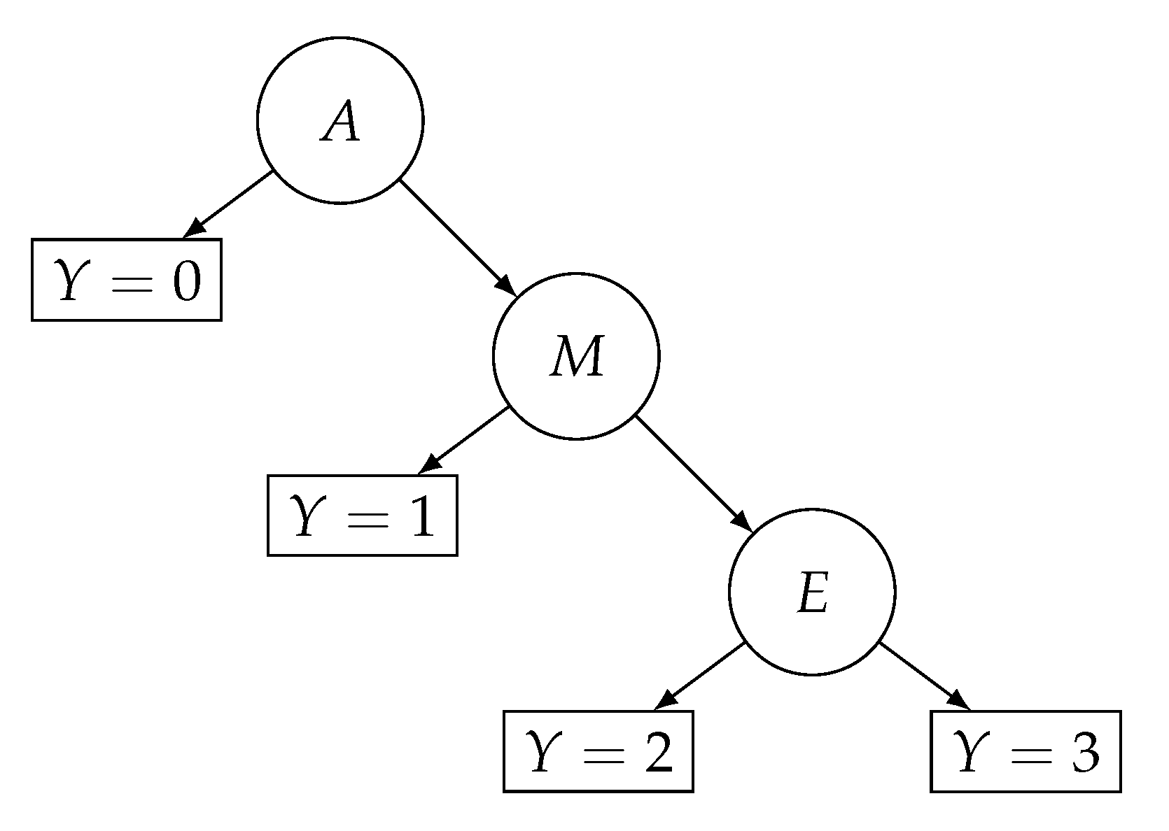
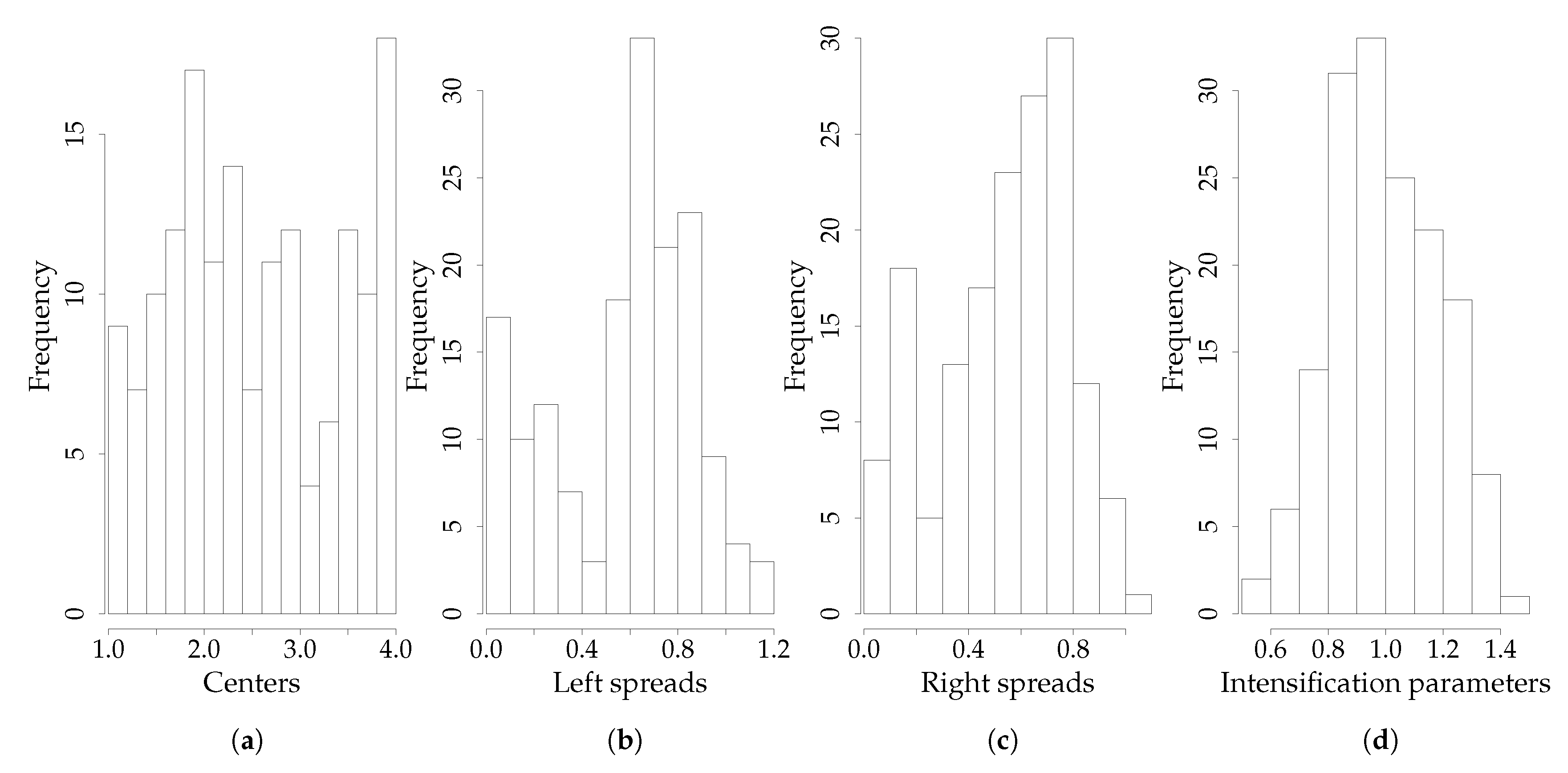
The matrices ${\mathbf{Y}}_{160\times 14}$ and ${\mathbf{T}}_{160\times 14}$ of the crisp rating responses and times have been used as input of the fIRTree procedure (see Section 2.2), which has produced as output the matrices ${\mathbf{C}}_{160\times 14}$, ${\mathbf{L}}_{160\times 14}$, ${\mathbf{R}}_{160\times 14}$, ${\mathbf{W}}_{160\times 14}$ of fuzzy parameters. For the sake of simplicity, the linear decision tree with three nodes has been used (see Figure 3). In this case, the response process is formalized by means of three nodes, namely node A for a first agreement/disagreement toward the item being assessed, node M for a moderate level of agreement/disagreement, and node E for the selection of extreme response categories. The IRTree model has been defined using the R library IRTrees [15] whereas model parameters $\mathit{\alpha }$ and $\mathit{\eta }$ have been estimated using the R library glmmTMB [32]. Finally, estimated centers, left/right bounds, and intensification parameters of fuzzy numbers have been averaged in order to obtain a composite indicator for depression [10]. Figure 4 shows the histograms of the composite fuzzy indicator w.r.t. centers, left/right spreads, and intensification parameters. Note that the magnitude of left/right spreads (Figure 4b,c) shows that a certain level of fuzziness is present in ratings data, whereas the intensification parameter (Figure 3d) shows a higher concentration of values closed to one (21.25%, reference range: $[0.95,1.05]$). The fuzzy indicator depression has been considered as the response variable of the next statistical models. Three crisp predictors have been used as follows: (a) religiousness, a categorical variable with two categories $\{\mathtt{Yes},\mathtt{No}\}$; (ii) emotional_stability, a compound indicator about personality [33], which has been derived from the Ten Item Personality Inventory [33] as a convex combination of the items and Cronbach’s $\alpha$. The following formula has been used for the $\alpha$-based composite indicator:

$$\mathtt{emotional}\text{\_}{\mathtt{stability}}_i=\alpha \times \sum _{j=1}^J\mathtt{emotional}\text{\_}{\mathtt{stability}}_{ij}+(1-\alpha )\times mean\left(\sum _{j=1}^J\mathtt{emotional}\text{\_}{\mathtt{stability}}_{ij}\right)$$

Note that in this context the $\alpha$ coefficient is used to create a crisp composite indicator where the contribution of the single item is weighted by the overall internal consistency of the scale they belong to. This should not be confused with the fuzzy $\alpha$ coefficient provided by [34], which is instead used to assess the internal consistency of a fuzzy scale; (iii) university, a categorical variable with two categories $\{\mathtt{Yes},\mathtt{No}\}$, with $\mathtt{Yes}$ indicating the case where participants have reached the university education level.

3.2. Data Analysis and Results

In order to compare the results of the fuzzy approach to data analysis as opposed to the standard way of analyzing this data, a normal linear model and a log-normal linear model have been additionally defined and fit on the crisp indicators for depression and response times. In this respect, a traditional data analysis procedure would require to estimate two separate models, one for crisp ratings and a second one for the response times.

Table 1. Application: Estimates, standard errors, and CIs of the normal linear model on crisp ratings, log-normal linear model on response times, and the fuzzy normal linear model on the composite indicator depression. Note that the categorical variables have been codified with dummy coding with the following reference levels: religiousness (ref.: No) and university (ref.: No). For all the analyses, $\alpha =0.05$.

Models	$\widehat{\mathit{\beta }}$ (${\mathit{\sigma }}_{\widehat{\mathit{\beta }}}$)	(1 − $\mathit{\alpha }$%) CI
Normal Linear Model
Residuals quantiles: Q1: −0.555, Med: −0.041, Q3: 0.611
${\beta }_0$ (Intercept)	4.204 (0.211)	[3.788, 4.621]
religiousness (No vs. Yes)	−0.146 (0.135)	[−0.412, 0.120]
emotional_stability	−0.232 (0.029)	[−0.289, 0.174]
university (No vs. Yes)	−0.280 (0.119)	[−0.516, −0.044]
pseudo-$R^2=0.507$
Log-Normal Model
Residuals quantiles: Q1: −0.298, Med: −0.060, Q3: 2.427
${\beta }_0$ (Intercept)	0.138 (58.573)	[7.792, 8.336]
religiousness (No vs. Yes)	0.256 (0.088)	[0.083, 0.429]
emotional_stability	0.003 (0.019)	[−0.034, 0.041]
university (No vs. Yes)	0.162 (0.078)	[0.008, 0.316]
pseudo-$R^2=0.199$
Fuzzy Normal Linear Model
Residuals quantiles: Q1: −0.287, Med: 0.068, Q3: 0.737
${\beta }_0$ (Intercept)	3.383 (0.259)	[2.870,3.894]
religiousness (No vs. Yes)	−0.169 (0.152)	[−0.469,0.130]
emotional_stability	−0.127 (0.034)	[−0.195, −0.060]
university (No vs. Yes)	−0.172 (0.134)	[−0.436, 0.093]
pseudo-$R^2=0.304$

shows the estimated coefficients, standard errors and the associated confidence intervals (CIs) for the two linear models. In particular, the results indicate that depression decreased as a function of emotional_stability $(\widehat{\beta }=-0.232,{\sigma }_{\widehat{\beta }}=0.029,\mathrm{CI}=[-0.289,-0.174])$, religiousness ($\widehat{\beta }=-0.146,{\sigma }_{\widehat{\beta }}=0.135,\mathrm{CI}=[-0.412,0.120]$), and university ($\widehat{\beta }=-0.280,{\sigma }_{\widehat{\beta }}=0.119,\mathrm{CI}=[-0.516,-0.044]$). On the other hand, the results of log-normal linear model reveal a positive relationship between response times and emotional_stability ($exp(\widehat{\beta })=1.003,{\sigma }_{\widehat{\beta }}=0.019,\mathrm{CI}=[-0.034,0.041]$), religiousness ($exp(\widehat{\beta })=1.292,{\sigma }_{\widehat{\beta }}=0.088,\mathrm{CI}=[0.083,0.429]$), and university ($exp(\widehat{\beta })=1.176,{\sigma }_{\widehat{\beta }}=0.078,\mathrm{CI}=[0.008,0.316]$). Considering that participants dedicating a larger amount of time to respond might show a more uncertain response process [35], religious and highly educated participants seem to provide more uncertain responses as opposed to not religious and less educated participants. Overall, the results of traditional data analysis are consistent with the literature (e.g., see [36,37,38]). However, as a result of the two-stage data analysis, two issues might affect the overall validity and generalization of the results, namely the need of a correction for multiple testing and the bias that could potentially affect the inferential results of both the linear models. Note that these two limitations derive from the fact that the linear models being used to analyze ratings and response times entail independent inferential tests.

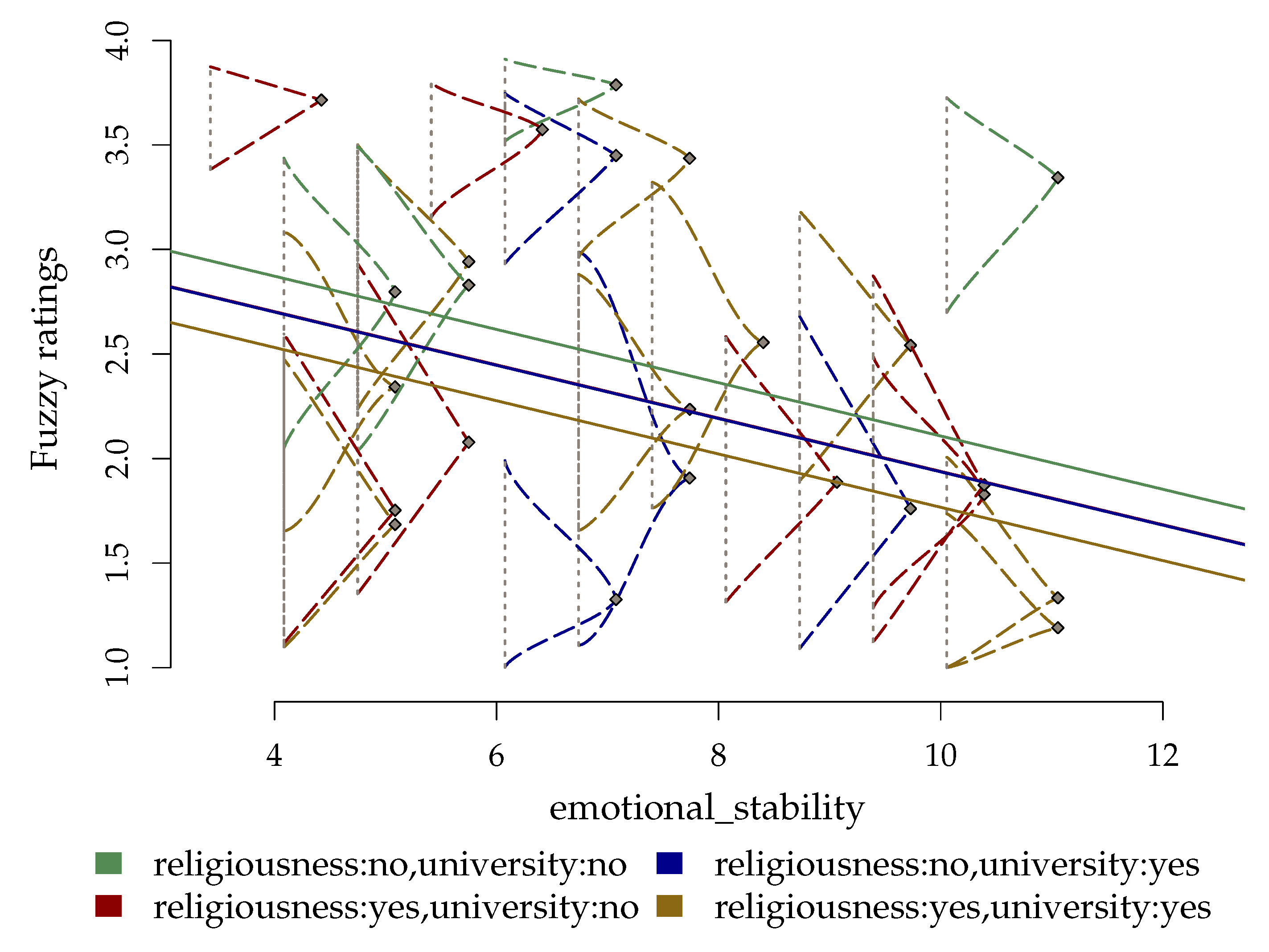
On the contrary, fuzzy data analysis can provide a unique statistical representation for the analysis and interpretation of both ratings data and response times. Unlike for the previous case, a single (fuzzy) linear normal model is instead used, where response times have been integrated via the intensification parameter of the fuzzy sets. Table 1 shows the results for this model. Overall, there is a significant negative relationship between depression and emotional_stability $(\widehat{\beta }=-0.128,{\sigma }_{\widehat{\beta }}=0.034,\mathrm{CI}=[-0.195,-0.060])$, with a larger effect of religiousness $(\widehat{\beta }=-0.170,{\sigma }_{\widehat{\beta }}=0.151,\mathrm{CI}=[-0.468,0.127])$, and university $(\widehat{\beta }=-0.172,{\sigma }_{\widehat{\beta }}=0.133,\mathrm{CI}=[-0.434,0.090])$. Interestingly, the goodness-of-fit indices (i.e., the pseudo-$R^2$s [39]) of the fuzzy normal linear model show quite different results from those of the of normal linear model. Indeed, the pseudo-$R^2$ for the fuzzy normal linear model (pseudo-$R^2=0.304$) seems to average the indices of the normal (pseudo-$R^2=0.507$) and log-normal (pseudo-$R^2=0.199$) linear models. In order to assess whether the temporal component of the ratings data plays a role in this case, an additional fuzzy normal linear model has been defined and fit, with the matrix $\mathbf{W}$ being set equal to one (i.e., $\mathbf{W}={\mathbf{1}}_{160\times 14}$). The goodness-of-fit index for this model shows a goodness-of-fit index quite closed to that of the previously estimated model (pseudo-$R_{\mathbf{W}=\mathbf{1}}^2=0.306$, pseudo-$R_{\mathbf{W}\ne \mathbf{1}}^2=0.304$), which would indicate that response times provide a marginal contribution in the analysis of depression. Finally, Figure 5 plots the fitted lines against the observed fuzzy ratings as a function of the predictors.

4. Conclusions

In this article we have provided initial findings to the problem of analyzing ratings data and response times with fuzzy numbers. This constitutes a crucial problem, especially when researchers need to evaluate the subjective component of questionnaire and survey data. A novel fuzzy rating procedure has been used (fIRTree), which allows for combining a probabilistic model of rater’s uncertainty and response times in a unique fuzzy representation. The novelty of the solution lies in the fact that response times and ratings data can be integrated using a common formal representation, which is in turn easy to interpret and use. A real case study has been discussed to highlight the characteristics of the proposed approach and a proper fuzzy data analysis has been adopted. Unlike for standard data analyses on ratings and response times, the proposed procedure is more parsimonious with regard to the number of statistical analyses because it requires estimating a single statistical model instead of two separated models for crisp ratings and response times and the number of hypothesis testing procedures preserves the interpretation of the inferential results by using single linear tests on model’s results. However, the fIRTree-based application has been focused on personality questionnaire data only, as they provide a more natural context for interpreting ratings data. Further studies might also include cognitive test-based data, which provide a well-suited framework for the joint modeling of responses and times [40]. In a similar way, additional studies might also evaluate the extension of fuzzy linear models to cope with the non-negativity of fuzzy responses, such as gamma or ex-Gaussian fuzzy linear models. Considering the mapping between empirical data (i.e., rating responses, response times) and fuzzy numbers, a fully fuzzy solution based on fuzzy inferential systems might be used in order to map fuzzy numbers and empirical data. For instance, this could potentially improve the overall interpretability of the proposed method.

References

- Schwarz, N.; Oyserman, D. Asking questions about behavior: Cognition, communication, and questionnaire construction. Am. J. Eval. 2001, 22, 127–160. [Google Scholar] [CrossRef] [Green Version]
- Tourangeau, R.; Rips, L.J.; Rasinski, K. The Psychology of Survey Response; Cambridge University Press: Cambridge, MA, USA, 2000. [Google Scholar]
- Rosenbaum, P.J.; Valsiner, J. The un-making of a method: From rating scales to the study of psychological processes. Theory Psychol. 2011, 21, 47–65. [Google Scholar] [CrossRef]
- Calcagnì, A.; Lombardi, L. Modeling random and non-random decision uncertainty in ratings data: A fuzzy beta model. AStA Adv. Stat. Anal. 2022, 106, 145–173. [Google Scholar] [CrossRef]
- Hesketh, T.; Pryor, R.; Hesketh, B. An application of a computerized fuzzy graphic rating scale to the psychological measurement of individual differences. Int. J. Man-Mach. Stud. 1988, 29, 21–35. [Google Scholar] [CrossRef]
- de Sáa, S.D.L.R.; Gil, M.Á.; Gonzalez-Rodriguez, G.; López, M.T.; Lubiano, M.A. Fuzzy rating scale-based questionnaires and their statistical analysis. IEEE Trans. Fuzzy Syst. 2014, 23, 111–126. [Google Scholar] [CrossRef]
- Calcagnì, A.; Lombardi, L. Dynamic Fuzzy Rating Tracker (DYFRAT): A novel methodology for modeling real-time dynamic cognitive processes in rating scales. Appl. Soft Comput. 2014, 24, 948–961. [Google Scholar] [CrossRef]
- Li, Q. Indirect membership function assignment based on ordinal regression. J. Appl. Stat. 2016, 43, 441–460. [Google Scholar] [CrossRef]
- Lalla, M.; Facchinetti, G.; Mastroleo, G. Ordinal scales and fuzzy set systems to measure agreement: An application to the evaluation of teaching activity. Qual. Quant. 2005, 38, 577–601. [Google Scholar] [CrossRef]
- Yu, S.C.; Yu, M.N. Fuzzy partial credit scaling: A valid approach for scoring the Beck Depression Inventory. Soc. Behav. Personal. Int. J. 2007, 35, 1163–1172. [Google Scholar] [CrossRef]
- Costas, C.S.L.; Maranon, P.P.; Cabrera, J.A.H. Application of diffuse measurement to the evaluation of psychological structures. Qual. Quant. 1994, 28, 305–313. [Google Scholar] [CrossRef]
- Chen, P.Y.; Yao, G. Measuring quality of life with fuzzy numbers: In the perspectives of reliability, validity, measurement invariance, and feasibility. Qual. Life Res. 2015, 24, 781–785. [Google Scholar] [CrossRef] [PubMed]
- Calcagnì, A. fIRTree: An Item Response Theory modeling of fuzzy rating data. arXiv 2021, arXiv:2102.02025. [Google Scholar]
- Calcagnì, A.; Cao, N.; Rubaltelli, E.; Lombardi, L. A psychometric modeling approach to fuzzy rating data. Fuzzy Sets Syst. 2022; in press. [Google Scholar] [CrossRef]
- Boeck, P.D.; Partchev, I. IRTrees: Tree-Based Item Response Models of the GLMM Family. J. Stat. Soft. 2012, 48, 1–28. [Google Scholar] [CrossRef] [Green Version]
- Dombi, J.; Jónás, T. Flexible fuzzy numbers for likert scale-based evaluations. In International Workshop Soft Computing Applications; Springer: Berlin/Heidelberg, Germany, 2018; pp. 81–101. [Google Scholar]
- Kyllonen, P.C.; Zu, J. Use of response time for measuring cognitive ability. J. Intell. 2016, 4, 14. [Google Scholar] [CrossRef]
- Corral, N. The minimun inaccuracy fuzzy estimation: An extension of the maximum likelihood principle. Stochastica 1984, 8, 63–81. [Google Scholar]
- Kruse, R.; Borgelt, C.; Braune, C.; Mostaghim, S.; Steinbrecher, M. Fuzzy Data Analysis. In Computational Intelligence; Springer: Berlin/Heidelberg, Germany, 2016; pp. 431–456. [Google Scholar]
- Couso, I.; Borgelt, C.; Hullermeier, E.; Kruse, R. Fuzzy sets in data analysis: From statistical foundations to machine learning. IEEE Comput. Intell. Mag. 2019, 14, 31–44. [Google Scholar] [CrossRef]
- Chukhrova, N.; Johannssen, A. Fuzzy regression analysis: Systematic review and bibliography. Appl. Soft Comput. 2019, 84, 105708. [Google Scholar] [CrossRef]
- Couso, I.; Dubois, D. Statistical reasoning with set-valued information: Ontic vs. epistemic views. Int. J. Approx. Reason. 2014, 55, 1502–1518. [Google Scholar] [CrossRef]
- Gebhardt, J.; Gil, M.A.; Kruse, R. Fuzzy set-theoretic methods in statistics. In Fuzzy Sets in Decision Analysis, Operations Research and Statistics; Springer: Berlin/Heidelberg, Germany, 1998; pp. 311–347. [Google Scholar]
- Denœux, T. Maximum likelihood estimation from fuzzy data using the EM algorithm. Fuzzy Sets Syst. 2011, 183, 72–91. [Google Scholar] [CrossRef] [Green Version]
- Tóth, Z.E.; Jónás, T.; Dénes, R.V. Applying flexible fuzzy numbers for evaluating service features in healthcare–patients and employees in the focus. Total Qual. Manag. Bus. Excell. 2019, 30, S240–S254. [Google Scholar] [CrossRef]
- Nasibov, E.N.; Peker, S. On the nearest parametric approximation of a fuzzy number. Fuzzy Sets Syst. 2008, 159, 1365–1375. [Google Scholar] [CrossRef]
- Casey, M.M.; Tryon, W.W. Validating a double-press method for computer administration of personality inventory items. Psychol. Assess. 2001, 13, 521. [Google Scholar] [CrossRef]
- Mignault, A.; Marley, A.; Chaudhuri, A. Inverted-U effects generalize to the judgment of subjective properties of faces. Percept. Psychophys. 2008, 70, 1274–1288. [Google Scholar] [CrossRef] [PubMed]
- De Boeck, P.; Bakker, M.; Zwitser, R.; Nivard, M.; Hofman, A.; Tuerlinckx, F.; Partchev, I. The estimation of item response models with the lmer function from the lme4 package in R. J. Stat. Softw. 2011, 39, 1–28. [Google Scholar] [CrossRef] [Green Version]
- Jeon, M.; Boeck, P.D. A generalized item response tree model for psychological assessments. Behav. Res. Methods 2015, 48, 1070–1085. [Google Scholar] [CrossRef]
- Parkitny, L.; McAuley, J. The depression anxiety stress scale (DASS). J. Physiother. 2010, 56, 204. [Google Scholar] [CrossRef] [Green Version]
- Brooks, M.E.; Kristensen, K.; van Benthem, K.J.; Magnusson, A.; Berg, C.W.; Nielsen, A.; Skaug, H.J.; Maechler, M.; Bolker, B.M. glmmTMB Balances Speed and Flexibility Among Packages for Zero-inflated Generalized Linear Mixed Modeling. R J. 2017, 9, 378–400. [Google Scholar] [CrossRef] [Green Version]
- Gosling, S.D.; Rentfrow, P.J.; Swann, W.B., Jr. A very brief measure of the Big-Five personality domains. J. Res. Personal. 2003, 37, 504–528. [Google Scholar] [CrossRef]
- Lubiano, M.A.; García-Izquierdo, A.L.; Gil, M.Á. Fuzzy rating scales: Does internal consistency of a measurement scale benefit from coping with imprecision and individual differences in psychological rating? Inf. Sci. 2021, 550, 91–108. [Google Scholar] [CrossRef]
- Yan, T.; Tourangeau, R. Fast times and easy questions: The effects of age, experience and question complexity on web survey response times. Appl. Cogn. Psychol. Off. J. Soc. Appl. Res. Mem. Cogn. 2008, 22, 51–68. [Google Scholar] [CrossRef] [Green Version]
- Bjelland, I.; Krokstad, S.; Mykletun, A.; Dahl, A.A.; Tell, G.S.; Tambs, K. Does a higher educational level protect against anxiety and depression? The HUNT study. Soc. Sci. Med. 2008, 66, 1334–1345. [Google Scholar] [CrossRef] [PubMed]
- Koenig, H.G. Research on religion, spirituality, and mental health: A review. Can. J. Psychiatry 2009, 54, 283–291. [Google Scholar] [CrossRef] [PubMed] [Green Version]
- Kotov, R.; Gamez, W.; Schmidt, F.; Watson, D. Linking “big” personality traits to anxiety, depressive, and substance use disorders: A meta-analysis. Psychol. Bull. 2010, 136, 768. [Google Scholar] [CrossRef]
- Veall, M.R.; Zimmermann, K.F. Evaluating Pseudo-R2’s for binary probit models. Qual. Quant. 1994, 28, 151–164. [Google Scholar] [CrossRef] [Green Version]
- De Boeck, P.; Jeon, M. An overview of models for response times and processes in cognitive tests. Front. Psychol. 2019, 10, 102. [Google Scholar] [CrossRef] [Green Version]
Figure 1.
Exemplification of four-parameter triangular fuzzy numbers represented in terms of the parameter. Note that c, l, and r are the center, left, and right bounds, respectively.
Figure 2.
Example of IRTree of a rating scale with three (e.g., 0: Disagree; 1: Neutral; 2: Agree) or four (e.g., 1: Strongly Disagree; 2: Disagree; 3: Agree; 4: Strongly Agree) response categories.
Figure 3.
Application: Linear decision tree for the four response categories. Note that A, M, and E denote the decision nodes of disagreement, moderate agreement/disagreement, and extreme agreement, respectively.
Figure 4.
Application: Histograms of the parameters of composite fuzzy indicator depression. (a) Histogram of the centers distribution; (b) histogram of left spreads () distribution; (c) histogram of right spreads () distribution; (d) histogram of intensification parameters () distribution. Note that the intensification parameter shows a concentration closed to one.
Figure 5.
Application: Fitted regression lines against the observed fuzzy ratings as a function of both categorical and continuous predictors. Note that the four regression lines correspond to the four categorical levels of religiousness and university (the line associated with religiousness:yes ∧ university:no is overlapped with the line of religiousness:no ∧ university:yes).