
Analyzing an Epidemic of Human Infections with Two Strains of Zoonotic Virus


College of Computer and Information Sciences, Fujian Agriculture and Forestry University, Fuzhou 350002, China
*
Author to whom correspondence should be addressed.
Mathematics 2022, 10(7), 1037; https://0-doi-org.brum.beds.ac.uk/10.3390/math10071037
Submission received: 7 February 2022
/
Revised: 21 March 2022
/
Accepted: 22 March 2022
/
Published: 24 March 2022
(This article belongs to the Special Issue Modelling and Control in Healthcare and Biology)
Abstract
:Due to the existence and variation of various viruses, an epidemic in which different strains spread at the same time will occur. here, an avian–human epidemic model with two strain viruses are established and analyzed. Both theoretical and simulation results reveal that the mixed infections intensify the epidemic and the dynamics become more complex and sensitive. There are six equilibria. The trivial equilibrium point is a high-order singular point and will undergo the transcritical bifurcations to bifurcate three equilibria. The existence and stability of equilibria mainly depend on five thresholds. A bifurcation portrait for the existence and stability of equilibria is presented. Simulations suggest that the key control measure is to develop the identification technology to eliminate the poultry infected with a high pathogenic virus preferentially, then the infected poultry with a low pathogenic virus in the recruitment and on farms. Controlling contact between human and poultry can effectively restrain the epidemic and controlling contagions in poultry can avoid great infection in humans.
1. Introduction
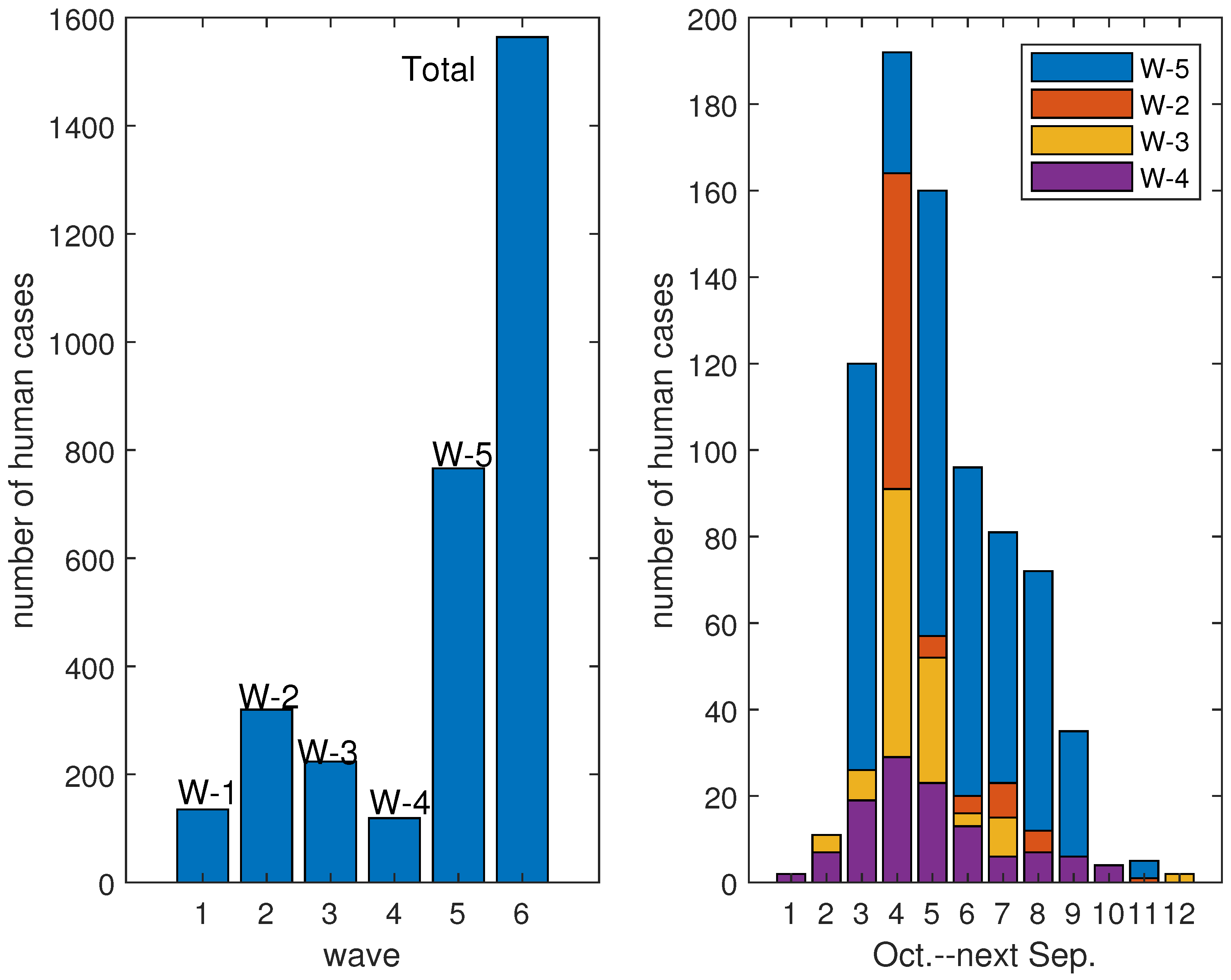
In recent years, the number of new and recurrent high-threat pathogens has increased, such as SARS-CoV, MERS-CoV, Ebola virus, Nipa virus, avian influenza virus and the latest, SARS-CoV-2. Among them, avian influenza and other zoonotic influenza have always been the great threat to human beings. Take human infection with H5N1 and H7N9 avian influenza as examples. In 1997, Hong Kong Special Administrative Region of China reported cases of human infection with high pathogenic H5N1 avian influenza virus. Since 2003, this avian influenza virus has spread from Asia to Europe and Africa, and is deeply rooted in poultry in some countries. Other subtypes of A(H5) avian influenza viruses also cause poultry epidemics and human infection. Regarding H7N9, the A(H7N9) virus has been detected in birds for many years and had not attracted people’s attention because of its low pathogenicity for birds and no previous record of human infections. However, the first human case was confirmed in March 2013 in China, before the epidemic of human infections with the A(H7N9) avian influenza virus broke out [1,2,3]. Successively, the same epidemic happened every autumn–winter, and so far there have been five outbreaks. The wave of 2016–2017 was an epidemic of human infections with both low and high pathogenic A(H7N9) avian influenza virus; that is, the virus had mutated and both the original virus and the mutated virus infected humans and poultry simultaneously. In fact, the gene sequencing analysis of the viruses isolated from two human A(H7N9) cases in January 2017 showed that the amino acid insertion mutations happened and the A(H7N9) virus had mutated into a high pathogenic virus for poultry [4]. Consequently, the number of cases and the fatality rate increased alarmingly. There were 1565 cases from 2013 to 2017 in total; however, the infection number was 766 in the wave of 2016–2017 [3]. It contributed almost half of all cases in those years. Not only that, in December 2016, there were 106 cases of human infections in China, and there were 192 human cases, 79 of which died in January 2017 [5]. This shows that the number of cases in a single month exceeds that of every past year and there were obviously more deaths. Infections during these five waves are presented in Figure 1.
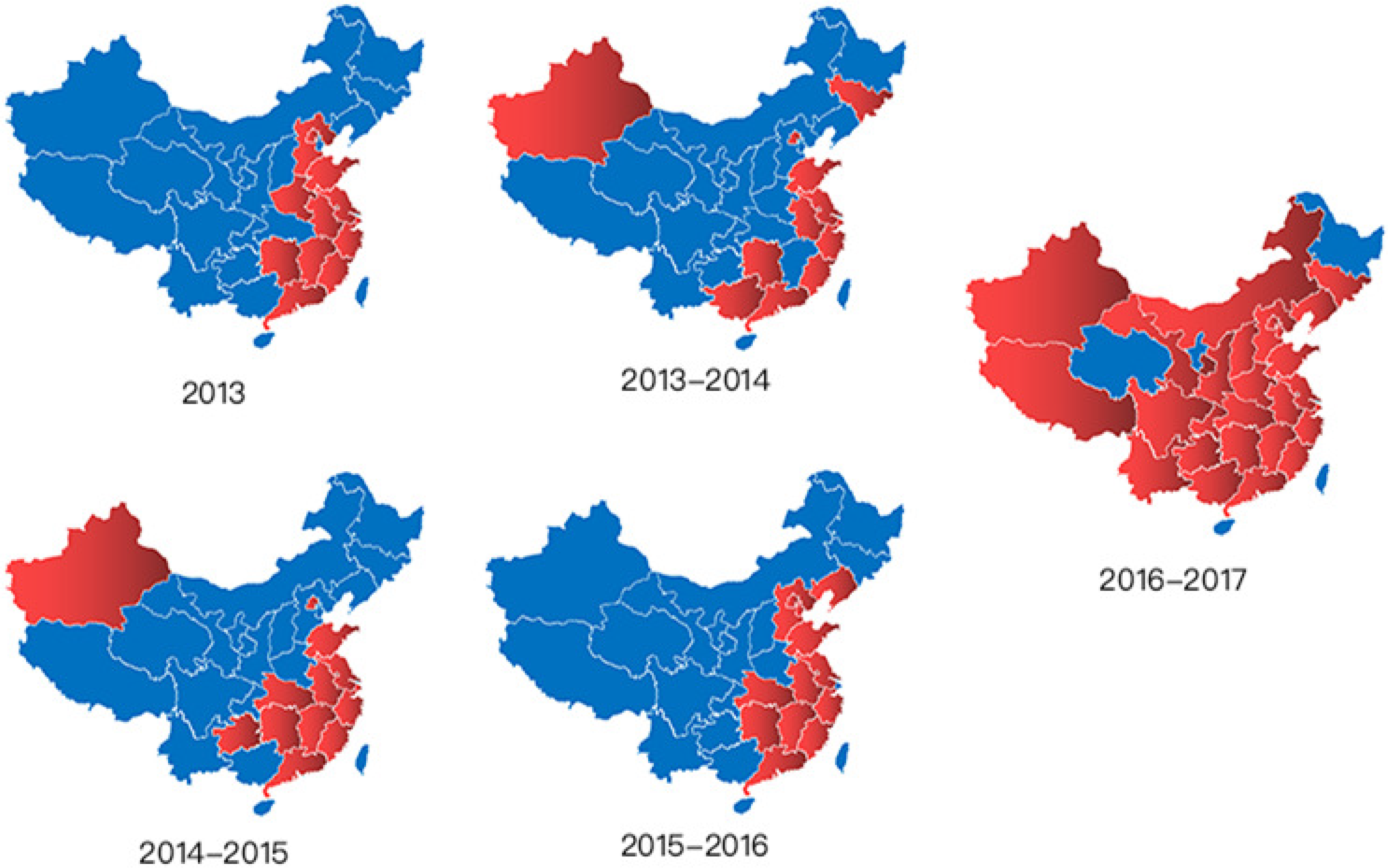
As well as the number of cases, the geographical distribution of cases in the wave of 2016–2017 was also far more than any previous wave. There were 12, 12, 13, 14 and 27 provinces, cities and municipalities with infections, respectively. Details are listed in Table A1 in Appendix A.1 and in Figure 2. We can see from Figure 2 that infections began in the coastal cities of the southeast China and had a tendency to expand vertically and to the inland regions. It also can be seen that the epidemic scope of the first four waves is relatively limited and fixed, while in the fifth wave there were human cases in almost all of the country, which suggests that the epidemic had expanded extensively and unusually.
Multiple strains are circulating in poultry, which makes it possible for human beings to be infected by different strains at the same time. Moreover, the increased number and the expanded geographical distribution in the fifth wave of human infections with the A(H7N9) avian influenza emphasize that it is well worth studying the spread and control of an epidemic of human infections with two strains of zoonotic influenza. Avian influenza viruses are classified as low pathogenic avian influenza (LPAI) viruses and high pathogenic avian influenza (HPAI) viruses according to their ability to cause disease in poultry. In view of their great threat to public health, there has been much research concerning the corresponding issues of genetic analysis, epidemiology and disease control. Arunachalam [6] found out the selection pressure of each amino acid site with the purpose of helping to develop effective vaccines and drugs for the A(H7N9) virus. Zhang et al. [7] discussed the occurrence of human infections with the A(H7N9) virus. Xing et al. [8] investigated the recurrent factors of the outbreak. Guo et al. [9] implemented the global dynamics of an avian–human influenza model. Li et al. [10] also obtained global stabilities of an A(H7N9) transmission model. Authors of this article, in their previous research [11,12] paid attention to the transmission of the virus in the environment. These studies were mainly finished before 2017 and focused on human infection with the low pathogenic avian influenza (LPAI). As we emphasize the simultaneous transmission of multiple viruses, we will take human infections with both the low and high A(H7N9) avian influenza viruses as an example to carry out this investigation. There are several studies concerning the transmission of two strains. For example, Tuncer et al. [13] introduced the dynamics of low and high pathogenic avian influenza in wild and domestic bird populations but emphasized that LPAI and HPAI can coexist in both populations. Kuddus et al. [14] investigated a two-strain disease model to simulate the prevalence of drug-susceptible and drug-resistant disease strains. In the present investigation, more complex and sensitive dynamics will be given out and the key control measures in the case of human infection with two strains of zoonotic virus also will be proposed.
The organization of this paper is as follows. In Section 2, we establish a mathematical model of avian–human infections in the fifth wave in mainland China. In Section 3, the existence of equilibria are investigated. Thresholds and the bifurcation portrait are given. In Section 4, local and global stabilities of equilibria are discussed dynamically. In Section 5, numerical simulations are implemented to clarify the dynamics of the model and the effect of control measures, and to carry out some comparative studies on human infections with low pathogenic, high pathogenic and mixed A(H7N9) viruses. In Section 6, we end this paper with conclusions and discussions.
2. The Model
In the present paper, the density of susceptible poultry population is denoted by , the density of infected poultry with low pathogenic A(H7N9) virus is denoted by because of very mild or no disease symptoms and the density of infected poultry with high pathogenic A(H7N9) virus is denoted by . . Densities of susceptible, infected and recovered human population are denoted by , and , respectively.
In view of biosafety, the implemented practical measures are to close the live poultry markets (LPMs) and to kill all the poultry within 3 kilometers of the outbreak, which would severely knock down the poultry industry and cause huge economic loss. In fact, the positive rates of H5, H7 and H9 in farms are far less than that in the live poultry markets. Yan et al. in [15], Zhu et al. in [16] and Cao et al. in [17] were all convinced that the positive rate in live poultry markets was much higher than that in poultry farms. Chen et al. in [18], noted that 44.4% of retail LPMs and 50.0% of wholesale LPMs were confirmed to be contaminated while no positive samples were detected from poultry farms. It seems that maintaining normal production can be considered in the outbreak. Therefore, we carry out our study with the premise of maintaining normal production. The following assumptions are made to establish the two-strain avian–human infection model:
Hypothesis 1 (H1).
Since we are considering normal production, the constant recruitment in poultry should be considered in the model. Moreover, in modern society, due to the expansion of people’s activities, migration is certain. Let and be the constant recruitment rate of poultry population and human population, respectively. Because the infected poultry with the high pathogenic A(H7N9) virus is easy to distinguish and the infected poultry with the low pathogenic A(H7N9) virus continues to show no disease symptoms, we consider that the susceptible and the infected poultry with the low pathogenic A(H7N9) virus are all included in the recruitment of poultry. represents the proportion of the latter in the recruitment.
Hypothesis 2 (H2).
The infected poultry with the low pathogenic A(H7N9) virus and the infected poultry with the high pathogenic A(H7N9) virus are all infectious, because they are carrying a virus.
Hypothesis 3 (H3).
Let be the output rate in the poultry industry including natural deaths and sales. is the natural death rate of the human population. is the additional death rate of due to infection with the high pathogenic A(H7N9) virus. is the extra death rate of human cases caused by disease. represents the recovery rate of human cases.
Hypothesis 4 (H4).
Suppose infections in poultry are due to contact. A saturated incidence function is used to describe the contact behaviors in poultry for the reason that the poultry population is large and densely populated. Because
and for the larger x, it is a monotonically increasing convex function and will reach saturation for the larger x. Therefore, it can express the saturated contact effect in poultry. x only represents the argument of the function. The corresponding infection rate functions are and .
Hypothesis 5 (H5).
As with human infections, many research results have confirmed that human behaviors, such as personal hygienic practice, reduced exposure to live poultry and disinfection of live poultry markets, will directly reduce the incidence of disease [19,20,21,22], because human behaviors will be affected by propaganda and psychosocial effects. At the beginning, human infections will expand due to people’s response lags. With the increase of human cases, the authorities concerned and mass media would respond and inform the public. Benefiting from protective awareness and behavioral changes, the incidence will decrease. Therefore, the incidence function from poultry to humans should satisfy , and will decrease when x is relatively large. Let , there is
Obviously, , and for the small x while for the larger x. In fact, will obtain the maximum value at which means the infections will increase at the beginning and then decrease after a certain time. The corresponding infection rate functions are and .
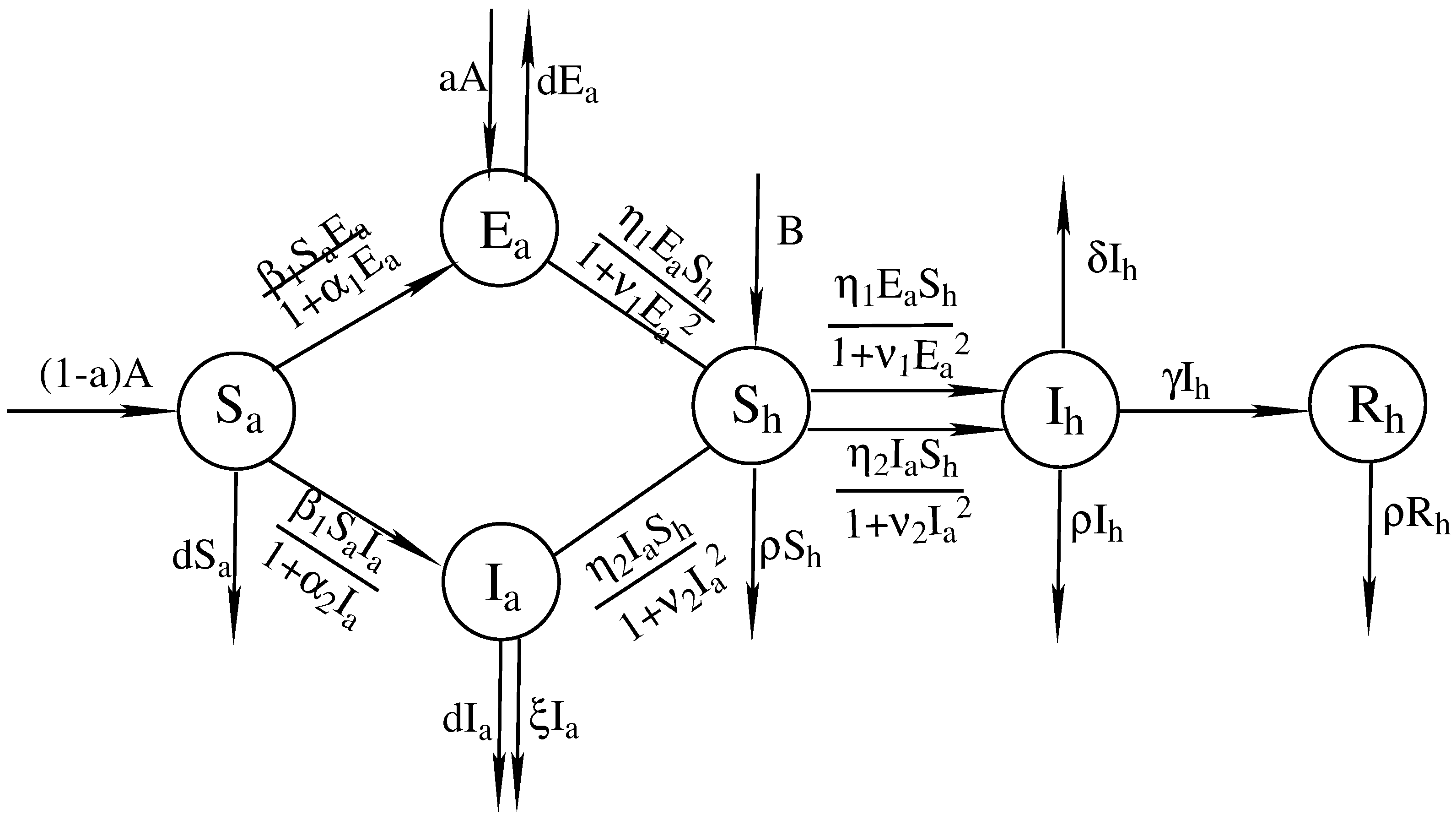
Based on the above analysis, the disease transmission mechanism is presented in Figure 3 and we establish the two-strain avian–human infection model as follows.
with the initial conditions .
It is obvious that all the solutions initiating in exist continuously for all and are unique. Where
Firstly, the biological validity should be guaranteed. Let Then, we have
By the differential inequality, we can obtain
Thus, and as
3. Existence of Equilibria
For a dynamic system, an equilibrium point corresponds to its constant solution. In epidemiology, equilibria can be classified as the disease-free equilibrium point and the disease-existence equilibrium point. Let us discuss the existence of equilibria firstly. As the constant solution of a differential equation , it can be obtained by solving the equation . Therefore, the Equilibria of System (1) depend on that of the system’s avian-subsystem which is as follows.
Natually, all solutions of System (2) that initiate in are confined in the region
for any and and System (2) is dissipative.
In view of solving equilibria, the third question of System (2) hints there is . Therefore, in the case of there is an axis equilibrium point and a boundary equilibrium point if , where . It is obvious that there is as . While in the case of , by the direct calculation, we can obtain
Denote
then and
According to the properties of quadratic function, Equation (3) has an unique positive root . Therefore, there is another boundary equilibrium point . Equation (3) also hints as . However, the existence of is conditional. ’s unconditional existence and ’s conditional existence indicate that it is possible to avoid the outbreak in poultry if we can put an end to the infected poultry in recruitment.
Suppose , then in the case of there is a boundary equilibrium point
under the condition of . It is obvious that as . If also , by the detailed calculation, we can obtain
then
From the expression of Equation (2), it can be seen that
then it should be and . Additionally, also should be satisfied. Therefore,
That is, there is a positive equilibrium point
In the case of , the equilibrium point also can be obtained from the second and third equations of System (2) by eliminating . Then there is
And
Therefore,
thus if . Hence exists if
Similarly,
and
Therefore, exists if
In the case of and , a direct calculation yields
Denote
then
It is obvious that if
Of course, if
Therefore, Equation (4) has an unique positive root . Furthermore
That is . Then, there is a positive equilibrium point with and . Therefore, it still requires . Thus, exists if
Equation (4) also hints as .
Denote
Noticing that if and , there are
Then as and .
Summarizing up, the equilibria and their existence conditions are listed in Table 1, and the corresponding conclusions are as follows:
Theorem 1.
- (i)
- Suppose , System (2) always has an axis equilibrium point ;And, there also exist two boundary equilibria if and if , where ;And, there is a positive equilibrium point if and , where .
- (ii)
- (iii)
- and as .
- (iv)
- if ; if ; if and .
Corollary 1.
As , System (2) has a positive equilibrium point if or .
Corollary 2.
undergoes the transcritical bifurcations to bifurcate equilibria and as increase from to .
By directly calculation, we also find that if ; if ; if ; if . The calculations are as follows:
Thus, there is
Corollary 3.
Suppose , System (2) has a positive equilibrium point if or .
As for these thresholds, there are the following relationships.
Details of the existence of equilibria are presented in Table 1.
The above results indicate that and exist with the larger and , respectively. will exist for larger , but the necessary existence conditions of may be stronger. In other words, the existence of is sensitive to parameters. Additionally, although and as , which we can detect from Equations (3) and (4), both the satisfied conditions are stronger. The reason is
The unequal relationship between the two ends of (5) corresponds to at , while the intermediate unequal relationship of (5) corresponds to . Moreover, exists unconditionally while exists if . In other words, these equilibria more likely to not exist if . It also indicates that it will be beneficial to disease control if we can eliminate the infected poultry in the recruitment.
Let be an equilibrium point of System (2), a direct calculation yields a corresponding equilibrium point of System (1), where
In the following, we will hold names of equilibria unchanged. Correspondingly, the existence of equilibria in System (1) is as follows.
Theorem 2.
Only the axis equilibrium point is the disease-free equilibrium point. All the boundary equilibria , and and the positive equilibria and are the disease-existence equilibria. Epidemiologically, the existence of a disease-free equilibrium point indicates that it is possible to eliminate the disease, the existence of a disease-existence equilibrium point means the disease may exist. Therefore, all and are thresholds of disease existence and the disease will exist with great probability. Results also indicate that we will do our best to put an end to the infected poultry in the recruitment and control the transmission in poultry so as to keep lower.
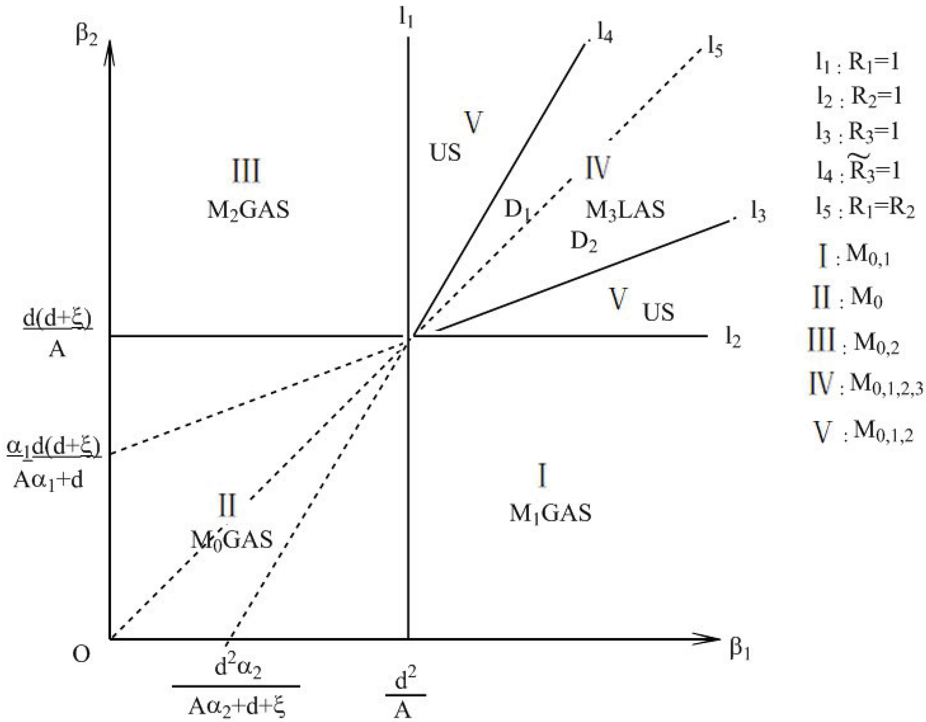
Dynamically, will undergo a series of transcritical bifurcations. will bifurcate an equilibrium point as increases from to and will bifurcate an equilibrium point as increases from to . also may bifurcate an equilibrium point as increase from to when and are satisfied. The bifurcation portrait of equilibria in the case of is depicted in Figure 4.
4. Stability of Equilibria
In terms of the dynamics of infectious disease, the stability of a disease-existence equilibrium point means the pandemic will occur, and the stability of a disease-free equilibrium point means the extinction of the disease. Now, we will discuss the stability of equilibria. Firstly, we investigate System (1). The Jacobian matrix of System (1) is given as
Denote
where
Therefore, J evaluated at every equilibrium point is stable if and only if so are H and Q as J is a block triangular matrix. Obviously, all the eigenvalues of the submatrix Q at every equilibrium point have the negative real parts, then the local stability of every equilibrium point depends on the evaluation of submatrix H. The Jacobian submatrix H corresponds to the poultry subsystem (2) which is independent of System (1). H evaluated at every equilibrium point is as follows, respectively.
The corresponding eigenvalues of at submatrix H are and . Then the axis equilibrium point is locally asymptotically stable (LAS) if thresholds and ; is an unstable saddle if the threshold or ; is locally stable if and or and because the unique zero eigenvalue is a simple eigenvalue; is a high-order singular point if and .
Because coordinates of satisfy the condition
then
For , there is . So that can characterize as
For the first second-order block matrix , it is easy to notice that there are two negative real part eigenvalues. Therefore, the local stability of either or depends on the sign of . Additionally Thus, and are all locally asymptotically stable (LAS) if the threshold .
Because satisfies , so that . Similarly, can characterize as
Moreover, the second-order block matrix , as the same reason that the local stability of depends on the sign of . And Thus, is locally asymptotically stable (LAS) if the threshold .
Similar to the above analysis, for , there are and . The Jacobian matrix can be characterized as
The corresponding characteristic polynomial is
where . Then
And the Routh–Hurwitz table is as follows.
where
| 1 | ||
| 0 | ||
| 0 |
Then
Therefore, items in the first column of the Routh–Hurwitz table are all positive. Thus by the Routh–Hurwitz criterion, all eigenvalues of the submatrix have negative real parts. That is, positive equilibra and are locally asymptotically stable if they exist.
Summarizing up the above analysis, we have following conclusions. Results are also represented in Table 2.
Theorem 3.
- (i)
- The axis equilibrium point is locally asymptotically stable if and ;
- (ii)
- is locally asymptotically stable if and ;
- (iii)
- is locally asymptotically stable if ;
- (iv)
- is locally asymptotically stable if and ;
- (v)
- is locally asymptotically stable if and ;
- (vi)
- is locally asymptotically stable if and .
The locally asymptotical stability of an equilibrium point means trajectories initiating in its neighborhood will converge to it eventually, which reflects the local dynamics of the system. Next, we will investigate the global stabilities of equilibria which will represent the global dynamics of the system. We investigate the avian subsystem (2) firstly. Choosing the Liapunov function , then
Therefore as . Let . By the LaSalle Invariance Principle, all solutions of the avian subsystem (2) will approach the plane.
Now, considering the limit system of the avian subsystem (2) about , we obtain
By theories of limit system, the stabilities of equilibria and convert to that of the corresponding limit system’s equilibria (still marked as and , respectively.). It is easy to obtain the corresponding equilibria , (as ) and of the limit system. Furthermore, is locally asymptotically stable as and , and are locally asymptotically stable as , respectively.
Next, we select the Dulac function , then
The Dulac criterion implies that the existence of periodic trajectories are excluded in the region . Therefore, by Poincaré-Bendixson theorem, equilibria and are globally asymptotically stable in , respectively. That is, is globally asymptotically stable as and ; is globally asymptotically stable as and ; is globally asymptotically stable as . Similarly, is also globally asymptotically stable as and .
Using the same discussion for the limiting human-subsystem, we can obtain the globally asymptotical stability of as and . Details can refer to the Appendix A.2. Therefore, by the LaSalle Invariance Principle and the theory of limit system, we can conclude that
Theorem 4.
- (i)
- is globally asymptotically stable as and or and ;
- (ii)
- is globally asymptotically stable as and ;
- (iii)
- is globally asymptotically stable as ;
- (iv)
- is globally asymptotically stable as and .
The globally asymptotical stability of a disease-free equilibrium point means the disease will be eradicated finally. This theorem tells us that for the lower and it is possible to eliminate the epidemic. Therefore, we should put an end to the infected individuals in the recruitment firstly, then try to control the spread of disease in poultry. Of course, properly reducing the circulation will help control the epidemic.
In the following, we will investigate global stabilities of positive equilibria and . Moreover, it suffices to discuss System (2). is the unique equilibrium point in as and there is an unique equilibrium point in as . Based on the above analysis, all solutions of System (2) are ultimately uniform bounded and System (2) is dissipative. Therefore, System (2) is uniformly persistent and domain is a bounded cone. That is, there is a compact subset .
Let be a function for x in an open set . Consider the differential equation
Denote as the solution of (6) with respect to . We make the following two basic assumptions of Equation (6):
Hypothesis 6 (H6).
There exists a compact absorbing set .
Hypothesis 7 (H7).
There exists an unique equilibrium point in .
Therefore, the System (2) satisfies conditions Hypotheses 6 and 7. In order to investigate the global stability of the positive equilibria, we introduce the Bendixson criterion [23]:
Let be an × matrix-valued function that is for .
Assume that exists and is continuous for . Denote
where the matrix is obtained by replacing each entry of P by its derivative in the direction of f, . is the second additive compound matrix [24,25] of the Jacobian matrix of f, is the Lozinskiľ measure of B with respect to a vector norm in , , defined by
A quantity q is defined as
Then,
Lemma 1
([23]). if is simply connected and the assumptions hold, the unique equilibrium point of (6) is globally stable in if .
Here, we denote the right hand of System (2) by with , the Jacobian matrix of System (2) has been listed above, its second additive compound matrix is
Define the function , then The matrix
where
Let be the vector in , we take a norm in as and denotes the Lozinskiľ measure with respect to this norm. By the method in Fiedler [24], we have , where
and are the matrix norms with respect to the vector norm, is the Lozinskiľ measure with respect to the norm.
There are
and
Because
Then
It is obvious that , and there are constants and independent of such that for because of the uniform persistence of the system. Then
Denote
Let , then .
Hence, by Lemma 1, we have or as . Then, we get the conclusion:
Theorem 5.
Either the positive equilibrium point (in the case of ) or (in the case of ) exists and will be globally asymptotically stable if .
The global stability of the positive equilibrium point means the pandemic will occur. Therefore, it is possible for the global stability of the disease-existence equilibrium point or for the larger and . Results also indicate the pandemic risk is increased if there is infected poultry in the recruitment.
Summing up the above analysis, the global stabilities of equilibria are presented in Table 2.
5. Simulations
In simulations, for mathematical convenience, we suppose , and . There are reports from the Chinese CDC that in April 2017, 8500 poultry in a farm in Hebei were infected with the new H7N9 and 5000 died; in May, 7500 poultry in a farm in Henan were infected and 5770 died; in a farm in Tianjin, 10,000 were infected and 6000 died; in a farm in Shangxi, were infected and 22,000 died; in a farm in Hohhot, Inner Mongolia, 59,556 were infected and 35,526 died; in June, in a farm in Batou, Inner Mongolia, 3850 were infected and 2056 died; in a farm in Heilongjiang, 20,150 were infected and 19,500 died, and so on. These data indicate that poultry can be infected with high pathogenic viruses in large numbers. Therefore, without loss of generality, we suppose . For an outbreak region, let us refer to A = 10,000 and . For poultry infection with the high pathogenic A(H7N9) virus, the extra death rate caused by the disease might be as well based on the above data. Poultry on farms usually are kept for 50 days in the farm industry in China, so the output rate is . The natural death rate of people can be given as as far as life expectancy is 75 years. The death rate of confirmed cases is about 40% and the treatment time of confirmed cases would be 15 days to 20 days according to documents from the Chinese CDC. Because the severe critical pneumonia mostly occurs about 3 to 7 days after the onset of the disease for a confirmed case, we may take an average of 5 days as reference, then the death rate due to disease is and the recovery rate is . Let as well.
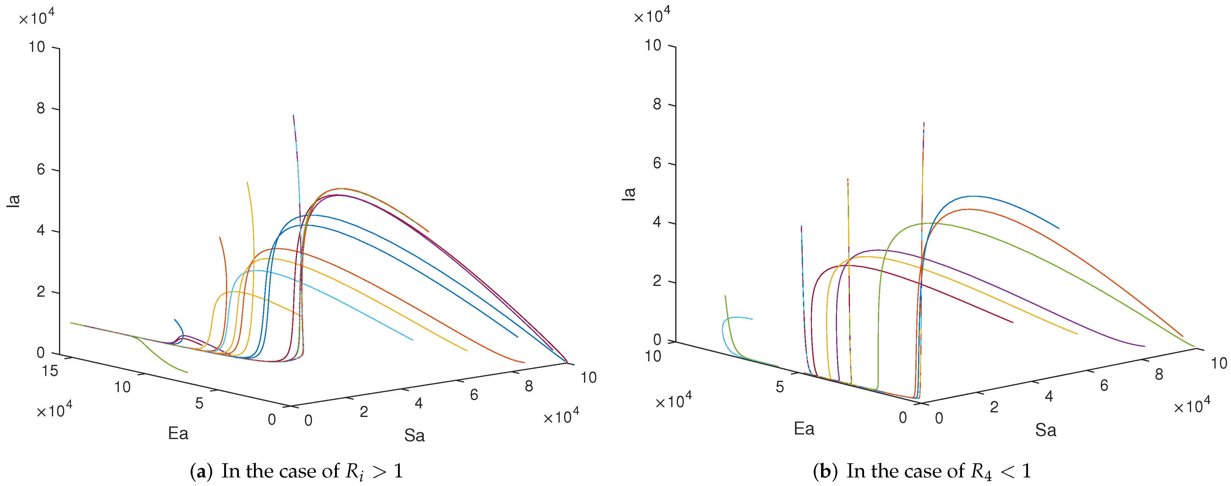
Now we carry out simulations with the purpose of investigating system dynamics, explaining control measures and doing some comparative studies for human infections with the low, high and mixed A(H7N9) viruses. Firstly, the dynamic behaviors of System (2) are illustrated in Figure 5. For the above parameters, all five thresholds are greater than 1 and it can be seen from Figure 5a that the positive equilibrium point is globally asymptotically stable. If we let , there is . Therefore, the positive equilibrium point does not exist and we can see from Figure 5b that the trajectories tend to the boundary equilibrium point .
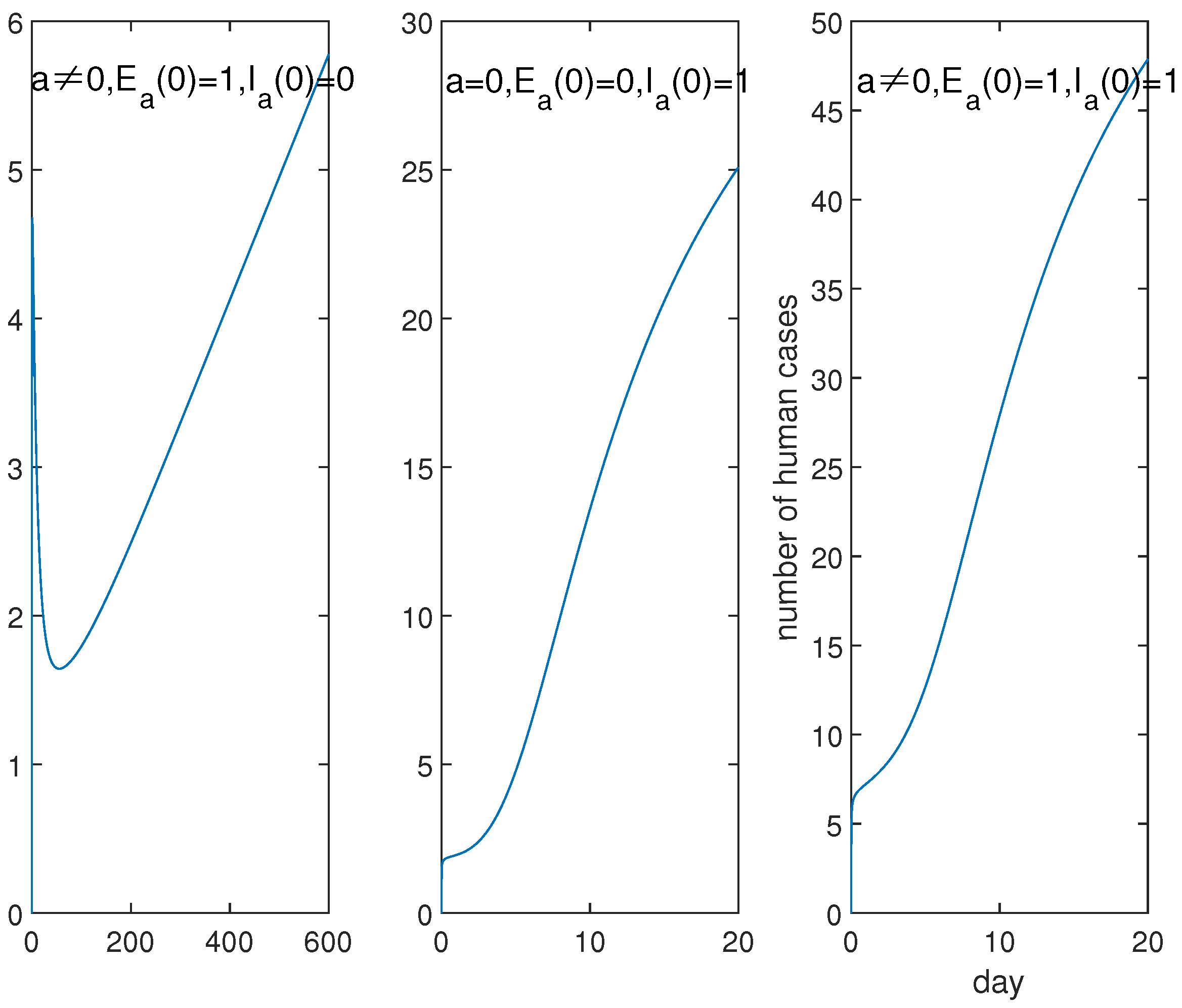
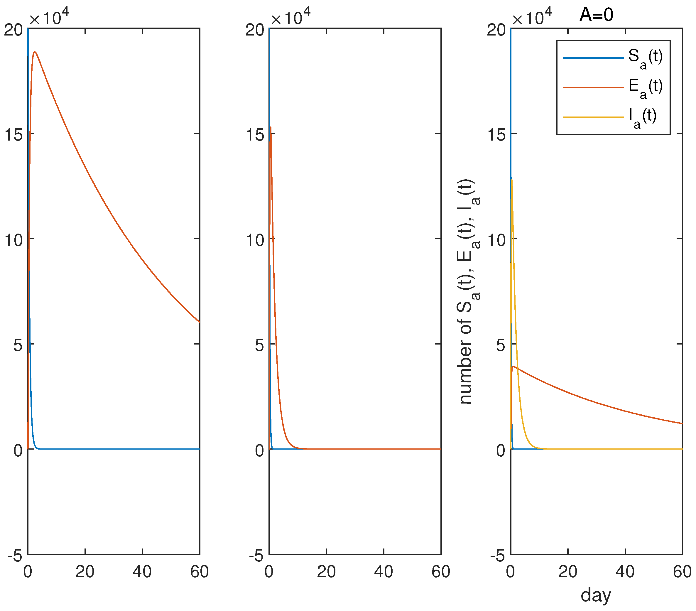
Furthermore, the dynamics of System (1) is depicted in Figure 6 which presents curves of for human infections with the low, high and mixed A(H7N9) viruses. We can see that the mixed A(H7N9) viruses will cause more serious infections than the other two, so the unusually serious epidemic in the fifth wave is explicated. The curve of corresponding to human infections with the low pathogenic A(H7N9) virus shows a different trend, that the curve will reach a small peak in a short time, then increase further after falling. This hints that people should respond quickly to control the epidemic before reinflating for the low pathogenic A(H7N9) infections. Moreover, it also suggests that human infection with the mixed A(H7N9) viruses is not the simple superposition of human infection with the low and high pathogenic A(H7N9) viruses.
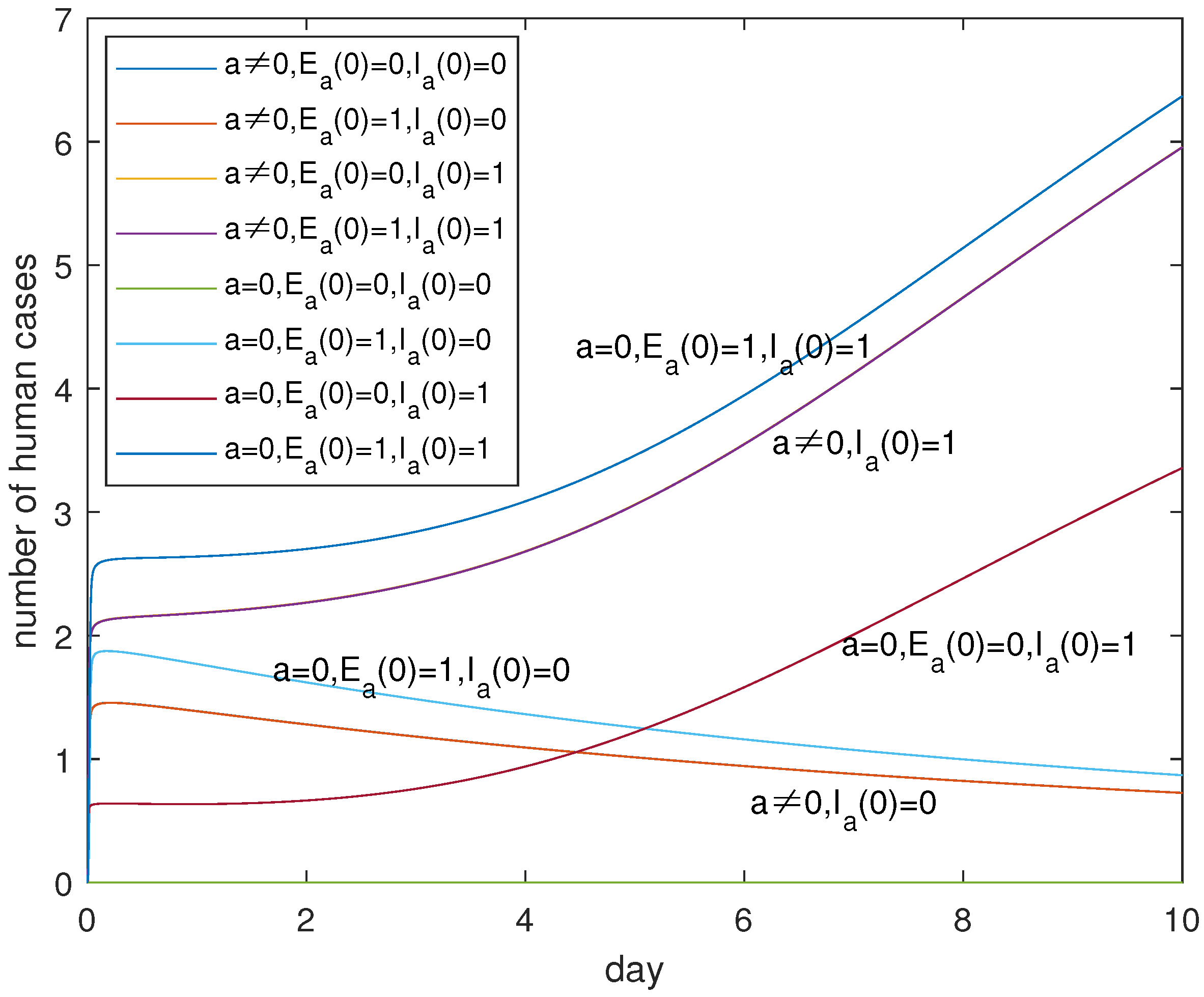
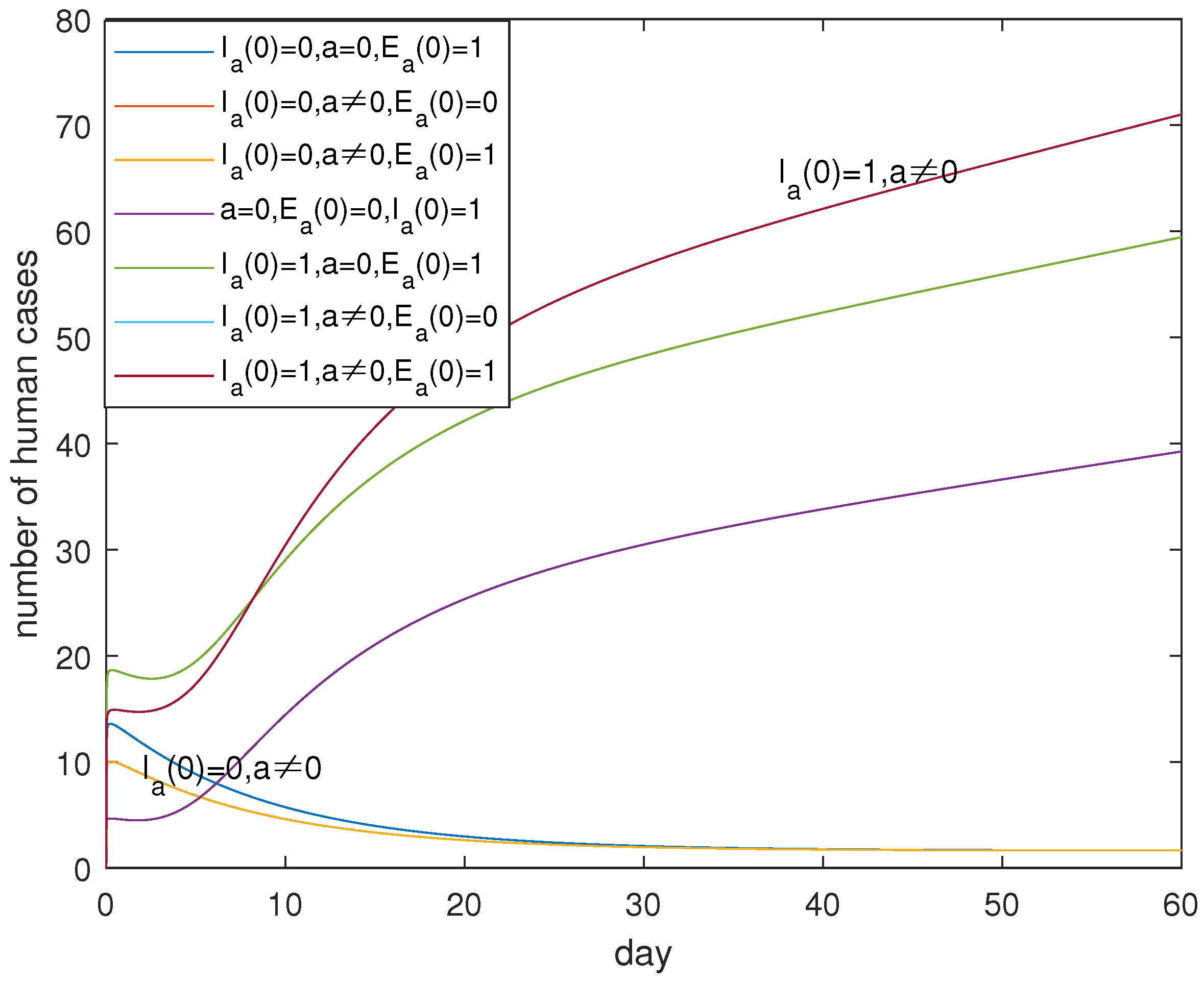
In view of the practical control measures, we can see from Figure 7 and Figure 8 that there are serious infections if , which can be detected from the representations of the three up curves and the two down curves which correspond to . This suggests that the more important thing is to identify and eliminate the infected poultry with the high pathogenic A(H7N9) virus. It is possible for us to eliminate the infected poultry with symptoms by killing and burying all sick poultry. As for the identification of infected poultry with low pathogenic A(H7N9) viruses on farms and in the recruitment, which one is more important? Figure 7 and Figure 8 tell us that it is different in the short term and in the long term, which can be extracted from the two down curves in Figure 7 and Figure 8. It seems that in the short term, the identification and elimination of the infected poultry on farms is prioritized. However, if we cannot eliminate the infected poultry with the low pathogenic A(H7N9) virus in the recruitment, there is no difference for or not which can be seen from the overlap curves. However, without the identification technology, it is also important to eliminate the infected poultry with the low pathogenic A(H7N9) virus in the recruitment which can be captured from the two up curves in Figure 8. In short, the identification technology is very important for the control of disease. It is more important for the identification of infected poultry with the high pathogenic A(H7N9) virus, than the infected poultry with the low pathogenic A(H7N9) virus on farms and in the recruitment.
From Figure 9 and Figure 10, we can see that the rapid infection of all poultry will occur whether by the low pathogenic virus or the high pathogenic virus. However, the infection caused by the low pathogenic virus of poultry to human beings far exceeds that caused by the high pathogenic virus in terms of time and quantity. There are two waves of human infections in the case of the mixed transmission. This may be the reason that the Chinese government decisively implemented strict vaccine measures against all poultry in the country when the mixed A(H7N9) infections seriously threatened people in 2017.
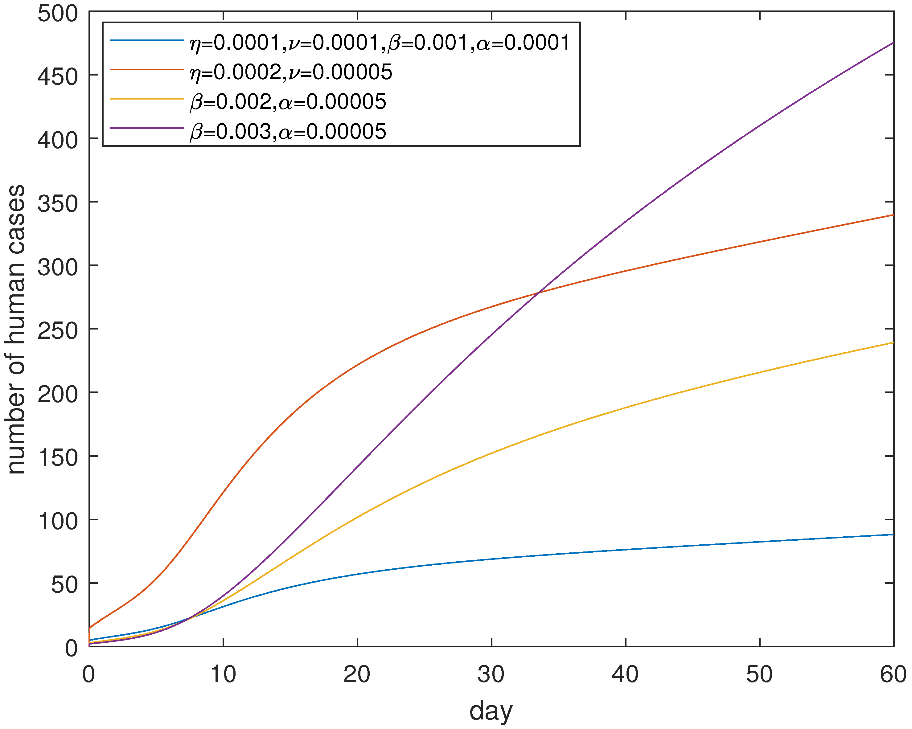
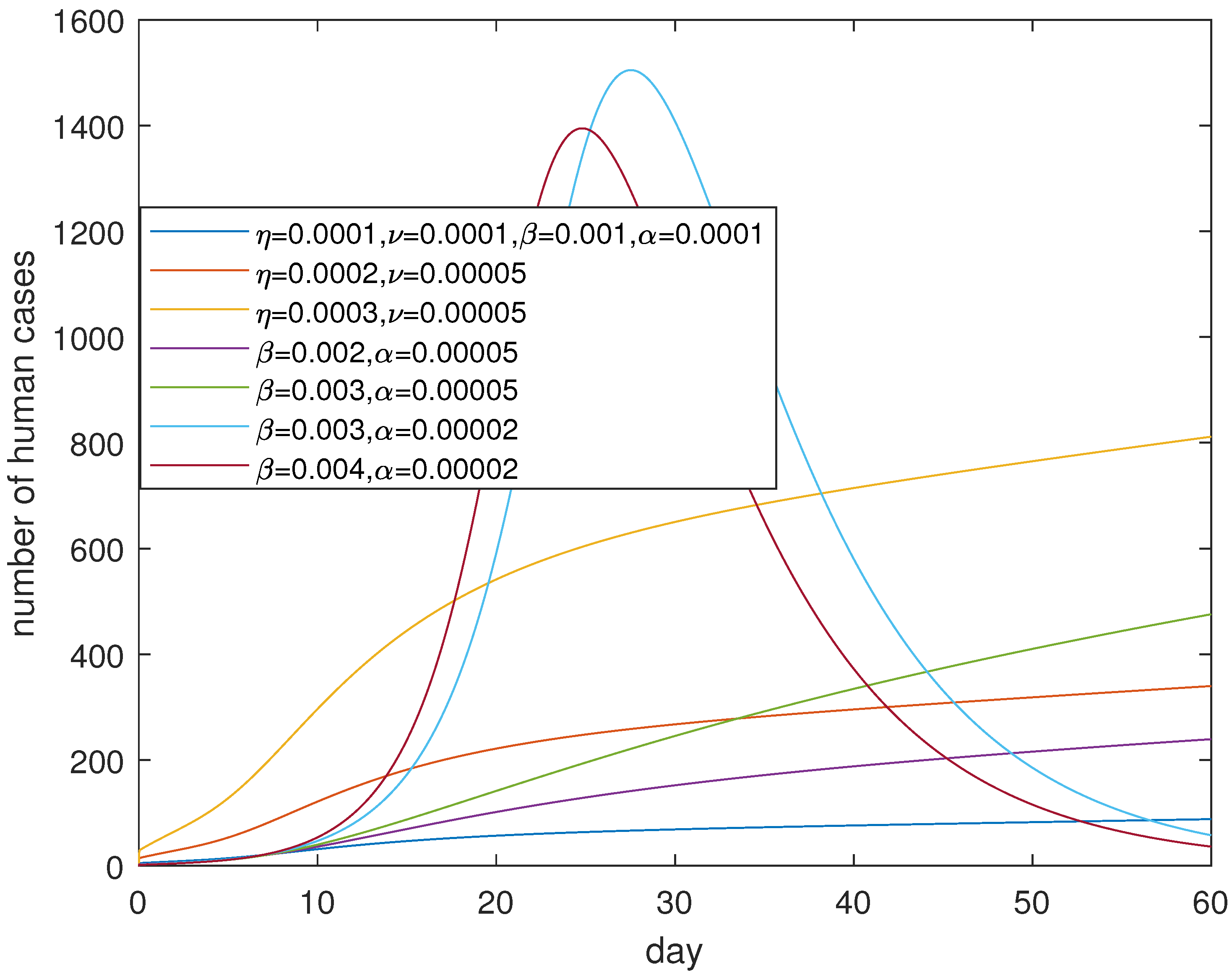
Figure 11 suggests that controlling contact both in poultry and between human and poultry can effectively control the epidemic in a month and losing controlling contacts in poultry will cause a serious pandemic. It seems it is very sensitive of parameters and embodying human response and the psychosocial effect, compared to parameters and which correspond to the transmission in poultry. Losing control of the contact between poultry will lead to a surge of human cases, which is depicted in Figure 12. Therefore, controlling the contact between poultry is as significant as controlling the contact for people with poultry. In short, we should respond immediately and take measures to reduce the contagions in poultry, and at the same time publicize the information so as to avoid the dangerous levels of exposure once a human case is confirmed.
6. Conclusions and Discussion
In 2013, the avian influenza A(H7N9) virus, which previously circulated only in poultry, began to infect humans. Hereafter, a new wave of epidemics emerged in every autumn and winter, severely discouraging the poultry industry and threatening public health. Frightened by the surge in number of human cases and the extension of the distribution of infected areas in the wave of 2016–2017, considering the fact that human infections with both the original low pathogenic and the newly emerging high pathogenic A(H7N9) viruses, we established and analyzed a two-strain avian–human infection model in order to investigate the dynamics of the epidemic, to explain and explore disease control measures and to make some comparative studies for human infections with the low or high pathogenic viruses and the mixed infections.
Because the low and high pathogenic A(H7N9) viruses are susceptible to both poultry and humans, the dynamics of the epidemic are more complex and sensitive. Theoretical results suggest there are four equilibria in the case of and two equilibria in the case of . In addition to the trivial equilibrium point , the others are all the disease-existence equilibria, including the boundary equilibria. It greatly increases the risk of pandemic. We also obtain the bifurcation portrait of the existence and stability of equilibria at . From the perspective of the existence conditions, basically equilibria and will exist for the larger . However, for the positive equilibrium point , the situation becomes more complicated, which also hints at the complex and sensitive nature of the dynamics. In fact, the existence of is not inevitable, which can be detected from the expressions of its existence thresholds. We also know the existing equilibria and in the case of will converge to the corresponding and at , although the required existence conditions are stronger. In any case, theoretically it is still the prior to eliminate the infected poultry in the recruitment so that , which may be beneficial to the disease eradication. The trivital equilibrium point is a high-order singular point as and and will bifurcates equilibria , and as increase from to . Of course, are the bifurcation thresholds. undergoes the transcritical bifurcations. Furthermore, if we can put an end to the infected poultry in recruitment, the stabilities of equilibria tell us that we have the possibility to eradicate the epidemic by controlling the transmission in poultry such that . The related results are presented in Theorems 1–3. The global stabilities of the positive equilibria and indicate again the importance of eliminating the infected poultry in recruitment which can be extracted from Theorem 4.
The implemented simulations verify the theoretical results and reveal that the dynamics of human infections with the low pathogenic A(H7N9) virus are different from that of the high pathogenic A(H7N9) virus and the mixed infections. The mixed low and high pathogenic A(H7N9) viruses would cause more serious infections in humans. Moreover, human infections with mixed low and high pathogenic A(H7N9) viruses is not the simple superposition of human infections with low and high pathogenic A(H7N9) viruses. For disease control, simulations suggest that the more important thing is to develop the identification technology to eliminate the infected poultry. Again, controlling the contact between human and poultry can effectively control the epidemic, and controlling the contagions in poultry can avoid a terrible rise in infections in humans. Evacuation stocking, isolated chicken houses and public notification mechanisms should be strengthened. This can give reference to the case of the simultaneous spreading of two strains between humans and poultry.
Because of the diversity of disease transmission, the widely used SEIR model is extended to include more categories of population, such as the asymptomatic, the hospitalized patients and the isolated individuals, etc. Additionally, more and more factors are also considered in modeling, such as medical resources, traffic power, contact behaviors, social and economic factors, and so on. Among these newly emerging models, it is worth mentioning those researches based on complex networks and networked populations. For example, Wang et al. in [26] gave a detailed and valuable introduction on epidemics in networked populations, which contributed the understanding of the complex networked disease transmission. Li et al. in [27] proposed a modified signed-susceptible-infectious-susceptible epidemiological model with positive and negative transmission rates and structural balance. Research on epidemic spreading via complex systems would be a successful way for us to face the challenge of disease transmission.
Obviously, this study is mainly focused on theoretical dynamics. In view of the realities of a complex epidemic, there are some factors which should be taken into account. For example, factor of the transmissions caused by the latent poultry infected with the high pathogenic virus should be considered, and the transmission via environment and objects should also be incorporated into models. From the point of view of disease control, the isolation of poultry production and trading/marketplaces are also worth considering. Therefore, further research will be carried out. There are also issues of the cotransmission and alternate prevalence of multivirulent strains in human seasonal influenza epidemic and the cross-transmission of sudden infectious diseases in the influenza season. In view of the interpersonal transmission of diseases, a networked approach will help to understand the spread of the disease. We will consider these in our subsequent research.
Author Contributions
Formal analysis, Y.C.; funding acquisition, Y.W. and Y.C.; data processing, H.Z., J.W., C.L. and N.Y.; writing, Y.C. All authors have read and agreed to the published version of the manuscript.
Funding
The National Natural Science Foundations of China (project no.: 32071892); The Natural Science Foundations of Fujian Province (project no.: 2021J01126).
Institutional Review Board Statement
Not applicable.
Informed Consent Statement
Not applicable.
Data Availability Statement
All data utilized in this paper are publicly available. Data and information of human infections with avian influenza A (H7N9) viruses were collected from World Health Organization, Centers for Disease Control and Prevention and Chinese Center for Disease Control and Prevention.
Acknowledgments
Authors are thankful to the learned reviewers for their useful suggestions and comments. Thanks for Song-Ying Li of University of California, Irvine, for his valuable comments. This work is also supported by China Scholarship Council (grant no. CSC201908350034). Finally, as a visiting scholar of University of California, Irvine, the first author thanks the Department of Mathematics in the School of Physical Sciences at the University of California, Irvine, for their space and hospitality.
Conflicts of Interest
The authors declare no conflict of interest.
Appendix A
Appendix A.1

Table A1.
Provinces, cities and municipalities where human cases occurred.
| Wave | Place |
|---|---|
| 1st | Shanghai, Anhui, Jiangsu, Zhejiang, Henan, Beijing, (Taiwan), Fujian, Hunan, Jiangxi, Shangdong, Hebei (2013.7), Guangdong (2013.7) |
| 2nd | New added: Guangxi, Jilin, Guizhou(back from Zhejiang), Hongkong, Xinjiang (2014.7); Not reappearing: Jiangxi, Henan, Hebei |
| 3rd | New added: Hubei, Guizhou; Not reappearing: Guangxi, Jixin, Henan, Hebei; Resumed: Jiangxi |
| 4th | New added: Tianjin, Liaoning; Not appearing: Xinjiang, Guizhou; Resumed: Hebei |
| 5th | New added: Sichuan, Yunnan, Tibet, Shaanxi, Shanxi, Chongqing, Gansu, Inner Mongolia, Macao |
Appendix A.2. The Global Stability of M2
Choosing the Liapunov function , then
Therefore as . Let . By the LaSalle Invariance Principle, all the solutions of the avian-subsystem (2) will approach the plane.
Now considering the limit system of the avian-subsystem (2) about , we obtain
Then by the theory of limit system, the stability of the equilibrium point converts to the stability of the corresponding equilibrium point (still marked as ) of the limit system. It is easy to obtain the corresponding equilibrium point (as ) and is locally asymptotically stable as and . Next, we select the Dulac function , then
The Dulac criterion implies that the existence of periodic trajectories are excluded in the region , Therefore, by Poincaré-Bendixson theorem the equilibrium point is globally asymptotically stable in . That is, is globally asymptotically stable as and .
Furthermore, we consider the limiting human sub-system
It is easy that
Therefore, is globally asymptotically stable as and .
References
- World Health Organization (WHO). Influenza (Avian and Other Zoonotic). Available online: https://www.who.int/en/news-room/fact-sheets/detail/influenza-(avian-and-other-zoonotic) (accessed on 23 November 2021).
- World Health Organization (WHO). Human Infection with Influenza A (H7N9) Virus in China. 2013-China. Available online: https://www.who.int/emergencies/disease-outbreak-news/item/2013_04_16-en (accessed on 23 November 2021).
- Centers for Disease Control and Prevention (CDC). Asian Lineage Avian Influenza A (H7N9) Virus. Available online: https://www.cdc.gov/flu/avianflu/h7n9-virus.htm (accessed on 23 November 2021).
- Chinese Center for Disease Control and Prevention (China CDC). Human Infection with H7N9 Avian Influenza. Epidemic Progress. A Mutant Strain of H7N9 Virus Was Found in Human Infection Cases in China. Available online: http://www.chinacdc.cn/jkzt/crb/zl/rgrgzbxqlgg/rgrqlgyp/201702/t20170220_138462.html (accessed on 23 November 2021).
- World Health Organization (WHO). Disease Outbreak News. Available online: https://www.who.int/emergencies/disease-outbreak-news/19 (accessed on 23 November 2021).
- Arunachalam, R. Adaptive evolution of a novel avian-origin influenza A/H7N9 virus. Genomics 2014, 104, 545–553. [Google Scholar] [PubMed]
- Zhang, J.; Jin, Z.; Sun, G.; Sun, X.; Wang, Y.; Huang, B. Determination of original infection source of H7N9 avian influenza by dynamical model. Sci. Rep. 2014, 4, 4846. [Google Scholar] [CrossRef] [PubMed] [Green Version]
- Xing, Y.; Song, L.; Sun, G.; Jin, Z.; Zhang, J. Assessing reappearance factors of H7N9 avian influenza in China. Appl. Math. Comput. 2017, 309, 192–204. [Google Scholar]
- Guo, S.; Wang, J.; Ghosh, M.; Li, X. Analysis of avian influenza A (H7N9) model based on the low pathogenicity in poultry. J. Biol. Syst. 2017, 25, 279–294. [Google Scholar]
- Li, Y.; Qin, P.; Zhang, J. Dynamics Analysis of Avian Influenza A (H7N9) Epidemic Model. Discret. Dyn. Nat. Soc. 2018, 2018, 7485310. [Google Scholar] [CrossRef] [Green Version]
- Chen, Y.; Wen, Y. Modelling and analyzing the epidemic of human infections with the avian influenza A (H7N9) virus in 2017 in China. Math. Methods Appl. Sci. 2019, 42, 4456–4471. [Google Scholar]
- Chen, Y.; Wen, Y. Spatiotemporal Distributions and Dynamics of Human Infections with the A H7N9 Avian Influenza Virus. Comput. Math. Methods Med. 2019, 2019, 9248246. [Google Scholar]
- Tuncer, N.; Torres, J.; Martcheva, M.; Barfield, M.; Holt, R. Dynamics of low and high pathogenic avian influenza in wild and domestic bird populations. J. Biol. Dynam. 2016, 10, 104–139. [Google Scholar]
- Kuddus, M.; McBryde, E.; Adekunle, A.; White, L.; Meehan, M. Mathematical analysis of a two-strain disease model with amplification. Chaos Solitons Fractals 2021, 143, 110594. [Google Scholar]
- Yan, Y.; Liu, H.; Jiang, L.; Shen, H. Positive rate and its influence factors of avian influenza A(H7N9) in poultry environment. Chin. Trop. Med. 2016, 16, 49–59. [Google Scholar]
- Zhu, B.; Huang, G.; Mai, W.; Tan, H.; Huang, X.; Chen, Z.; Lu, Z.; He, W.; Zhou, Y. Surveillance analysis on the high risk population and the distributional environment of avian influenza in zhaoqing from 2011 to 2013. Mod. Prev. Med. 2015, 42, 1386–1391. [Google Scholar]
- Cao, G.; Zhan, B.; Chen, X.; Feng, F. Surveillance of avian influenza virus in population with occupational exposure and in out-environment in Quzhou, Zhejiang. Dis. Surveill. 2013, 28, 884–887. [Google Scholar]
- Chen, Z.; Li, K.; Luo, L.; Lu, E.; Yuan, J.; Liu, H.; Lu, J.; Di, B.; Xiao, X.; Yang, Z. Detection of avian influenza A(H7N9) virus from live poultry markets in Guangzhou, China: A surveillance report. PLoS ONE 2014, 9, e107266. [Google Scholar]
- Bauch, C.; Galvani, A. Social factors in epidemiology. Science 2013, 342, 47–49. [Google Scholar]
- Funk, S.; Gilad, E.; Watkins, C.; Jansen, V. The spread of awareness and its impact on epidemic outbreaks. Proc. Natl. Acad. Sci. USA 2009, 106, 6872–6877. [Google Scholar]
- Xiang, N.; Shi, Y.; Wu, J.; Zhang, S.; Ye, M.; Peng, Z.; Zhou, L.; Zhou, H.; Liao, Q.; Huai, Y.; et al. Knowledge, attitudes and practices (KAP) relating to avian influenza in urban and rural areas of China. BMC Infect. Dis. 2010, 10, 34. [Google Scholar]
- Wang, L.; Cowling, B.; Wu, P.; Yu, J.; Li, F.; Zeng, L.; Wu, J.; Li, Z.; Leung, G. Yu, H. Human exposure to live poultry and psychological and behavioral responses to influenza A(H7N9), China. Emerg. Infect. Dis. 2014, 20, 1296–1305. [Google Scholar]
- Li, M.; Muldowney, J. A geometric approach to the global-stability problem. SIAM J. Math. Anal. 1996, 27, 1070–1083. [Google Scholar]
- Fiedler, M. Additive compound matrices and inequality for eigenvalues of stochastic matrices. Czech. Math. J. 1974, 99, 392–402. [Google Scholar]
- Muldowney, J. Compound matrices and ordinary differential equations. Rocky Mt. J. Math. 1990, 20, 857–872. [Google Scholar]
- Wang, Z.; Moreno, Y.; Boccaletti, S.; Perc, M. Vaccination and epidemics in networked populations—An introduction. Chaos Solitons Fractals 2017, 103, 177–183. [Google Scholar]
- Li, H.; Xu, W.; Song, S.; Wang, W.; Perc, M. The dynamics of epidemic spreading on signed networks. Chaos Solitons Fractals 2021, 151, 111294. [Google Scholar]
Figure 1.
Infections in the waves of human infections with avian influenza A(H7N9) virus.

Figure 2.
Geographical distributions of the previous five waves in mainland China. Remark: (1) The epidemic mainly occurred in mainland China, therefore there are only maps of mainland China. (2) It seems that all cases of Taiwan, Hong Kong and Macao were infected in mainland China, therefore they are not included when considering the geographical characteristics of disease transmission. (3) We depicted these graphics with the purpose of exploring the epidemic extension geographically in general, therefore the names of provinces, cities and municipalities are not marked. (4) Details of the provinces, cities and municipalities in which human cases were confirmed in every wave are listed in Table A1 in Appendix A.1. (5) The case in Guizhou in wave 2, a person who had just come back from Zhejiang, should be identified as infected in Zhejiang; therefore, Guizhou is excluded in the graphic for 2013–2014.

Figure 3.
The disease transmission mechanism.

Figure 4.
The bifurcation portrait of equilibria. . GAS—globally asymptotically stable; LAS—locally asymptotically stable; US—unstable.
Figure 4.
The bifurcation portrait of equilibria. . GAS—globally asymptotically stable; LAS—locally asymptotically stable; US—unstable.

Figure 5.
The dynamic behaviors of System (2) under different thresholds. (a) All trajectories converge to the positive equilibrium point, which means that the disease will be prevalent. (b) All trajectories tend to the plane, which hints that slowing down production and trade will help reduce the probability of mixed transmission.

Figure 6.
Dynamics for cases of LP, HP and the mixed infections. Left: cases of indicating corresponds to human infections with the low pathogenic A(H7N9) virus (LP); middle: cases of indicating corresponds to human infections with the high pathogenic A(H7N9) virus (HP); right: cases of corresponds to human infections with the mixed low and high pathogenic A(H7N9) viruses (Mixed). This suggests that the mixed low and high pathogenic A(H7N9) viruses will cause more serious infections in humans and that it is not the simple superposition of the LP and HP infections.

Figure 7.
Evolutions of for different initial values of and a within 10 days. Curves corresponding to cases of and are overlapping. Curves corresponding to cases of and are overlapping. It is very important to clear away high pathogenic infections in poultry, as shown by the rising and falling trend of the curve.

Figure 8.
Evolutions of for different initial values of and a in the longer days. Curves corresponding to cases of and are overlapping. Curves corresponding to cases of and are overlapping. The existence of poultry infected with the high pathogenic virus is the greatest threat to human beings, which can be seen from the rising trend of curves. Otherwise, the curve is descending.

Figure 9.
Evolutions of and for LP, HP and the mixed infections. From left to right are LP, HP and mixed infections, respectively. No matter whether the low pathogenic virus or the high pathogenic virus, the rapid infections of all poultry will occur. In the case of the mixed transmission, if the live poultry markets and farms are closed, a large number of deaths caused by the high pathogenic virus will greatly reduce the number of poultry infected with the low pathogenic virus.

Figure 10.
Evolutions of for LP, HP and the mixed infections. From left to right are LP, HP and the mixed infections, respectively. The infection rate caused by the low pathogenic virus of poultry to human beings far exceeds that caused by the high pathogenic virus in terms of time and quantity. Moreover, the mixed transmission will form two infection peaks.

Figure 11.
The effect of controlling both poultry–poultry and poultry–human contact. are the fixed parameters. When and are adjusted, the fixed and are unchanged; when and are adjusted, the fixed and are unchanged. The control effect of and may be better than the effect of and . The decreased and increased may effectively control the disease.

Figure 12.
Consequences of out of control. Losing control of contact and transmission in poultry will cause a large outbreak and lead to a human epidemic.
Figure 12.
Consequences of out of control. Losing control of contact and transmission in poultry will cause a large outbreak and lead to a human epidemic.

Table 1.
Existence of equilibria.
| Case | Equilibria | Threshold | Condition Characteristic | Remarks |
|---|---|---|---|---|
| None | Unconditional existence | |||
| For larger , exists. | ||||
| For larger , exists. | ||||
| , | , | For larger and , | ||
| , | , | may exist. | ||
| or | ||||
| or | ||||
| or | if | |||
| or | if | |||
| None | Unconditional existence | |||
| For larger , exists. |
Where .
Table 2.
Global stabilities of equilibria.
| Case | Equilibria | Stabilities and Conditions | Remarks |
|---|---|---|---|
| or | |||
| Exists if . | |||
| Exists if . | |||
| For larger and | |||
| and | Exists if and | ||
| For larger and | |||
| and | Exists if |
Publisher’s Note: MDPI stays neutral with regard to jurisdictional claims in published maps and institutional affiliations. |
© 2022 by the authors. Licensee MDPI, Basel, Switzerland. This article is an open access article distributed under the terms and conditions of the Creative Commons Attribution (CC BY) license (https://creativecommons.org/licenses/by/4.0/).
Share and Cite
MDPI and ACS Style
Chen, Y.; Zhang, H.; Wang, J.; Li, C.; Yi, N.; Wen, Y. Analyzing an Epidemic of Human Infections with Two Strains of Zoonotic Virus. Mathematics 2022, 10, 1037. https://0-doi-org.brum.beds.ac.uk/10.3390/math10071037
AMA Style
Chen Y, Zhang H, Wang J, Li C, Yi N, Wen Y. Analyzing an Epidemic of Human Infections with Two Strains of Zoonotic Virus. Mathematics. 2022; 10(7):1037. https://0-doi-org.brum.beds.ac.uk/10.3390/math10071037
Chicago/Turabian StyleChen, Yongxue, Hui Zhang, Jingyu Wang, Cheng Li, Ning Yi, and Yongxian Wen. 2022. "Analyzing an Epidemic of Human Infections with Two Strains of Zoonotic Virus" Mathematics 10, no. 7: 1037. https://0-doi-org.brum.beds.ac.uk/10.3390/math10071037
Note that from the first issue of 2016, this journal uses article numbers instead of page numbers. See further details here.