Advancing Multidisciplinary STEM Education with Mathematics for Future-Ready Quantum Algorithmic Literacy

Abstract

The perception that mathematics is difficult has always persisted. Nevertheless, mathematics is such an essential component of STEM education. Quantum technologies are already having enormous effects on our society, with advantages seen across a broad variety of industries, including finance, aerospace, and energy. These innovations promise to transform our lives. Managers in the business and public sectors will need to learn quantum computing. Quantum algorithmic literacy may help increase mathematical understanding and enthusiasm. The current paper proposes that one possible approach is to present the information in a reasonably gentle but intelligible way, in order to excite individuals with the mathematics that they already know by extending them to acquiring quantum algorithmic literacy. A gentle introduction to the mathematics required to model quantum computing ideas, including linear transformations and matrix algebra, will be given. Quantum entanglement, linear transformations, quantum cryptography, and quantum teleportation will be used as examples to illustrate the usefulness of basic mathematical concepts in formulating quantum algorithms. These exemplars in quantum algorithmic literacy can help to invigorate people’s interest in mathematics. Additionally, a qualitative comparative analysis (QCA) framework is provided that teachers can utilize to determine which students to approach for remediation. This assists the teachers in dispelling any pupils’ uncertainty about mathematical concepts.

1. Introduction

1.1. Quantum Algorithmic Literacy as an Approach for Igniting Interest in Mathematics

The advent of quantum technologies is already having positive impacts on humanity, with benefits that will be felt across a wide range of industries in the coming years, including the financial, defense, aerospace, and energy sectors [1]. When it comes to quantum computing, managers in the private sector and government will have to become quantum literate [2]. However, currently only a select group of scientists and mathematicians possess the abilities required for effective quantum computational reasoning via algorithms. While quantum computing offers an exciting new paradigm for tackling some of the most difficult challenges faced by humanity, only a small part of the population knows how these technologies work, and there are considerable perceived barriers to entry from outside the field. Science increasingly relies on the multi-disciplinarity of STEM to solve challenging problems which are complex and in multiple domains [3]. Such an endeavor requires a cross-disciplinary approach.

Quantum algorithmic literacy [4] is a possible approach to generating greater interest in mathematics. Having a working knowledge in mathematics to develop quantum algorithms can help to equip people with the tools needed to build innovative quantum solutions to the world’s greatest problems through cross-disciplinary collaboration.

1.2. Problem Statement: Mathematics Is Perceived as a Barrier to Quantum Algorithmic Literacy

There has been a long-standing (mis)perception regarding the difficulty of the STEM curriculum since mathematics plays such a crucial part, according to Yates and Millar [5]. There is a pedagogical angle to consider regarding “the barrier of mathematical knowledge required” in quantum theory. Yates and Millar argue that advanced concepts such as quantum physics need a high degree of mathematics. Mathematical notation such as the Dirac notation [6] and mathematical equations can convey quantum states and ideas, yet most people might not have encountered them. In order to excite people with the mathematics that they already know, the current paper submits that a viable strategy is to present the quantum algorithmic content in a relatively comprehensible manner.

1.3. Research Question

The overarching research question that guides this paper is: how can we make quantum algorithmic literacy in STEM education accessible to students with the basic foundational mathematics that they already know?

1.4. Organization of the Subsequent Sections

In the methods section, a basic understanding of the mathematics needed for modeling quantum computing-related algorithmic concepts, which includes linear transformations and matrix algebra, will be presented. Subsequently, in the sections Application of the Methods and Findings, exemplars of how to apply the basic mathematics in modeling quantum algorithmic concepts will be gently presented. The examples include quantum entanglement, linear transformations applied in quantum cryptography, and quantum teleportation.

2. Methods

2.1. A Basic Understanding of Mathematics for Modeling Quantum Mechanics

Quantum technologies are based on solid theoretical underpinnings in both physics and mathematics. Yuri Manin [7] and Paul Benioff [8] first proposed the notion of employing quantum systems as computing devices in the 1980s, although they conducted their research separately. Richard Feynman [9] famously expounded on this subject in 1982.

To grasp the distinction between classical and quantum computers, we shall look at some differences between them. Classical computers store their data as sequences of zeros and ones in the form of binary numbers. The bit is a logical unit of storage that may hold either 0 or 1. When discussing 0 and 1, it is helpful to think of them just as symbols. The quantum computer’s memory unit is referred to as a “qubit”, and it is capable of storing both 0 and 1. On a plane, a qubit’s value is a vector of length 1.

A link with a classical bit is established by designating one axis of a coordinate system with the symbol 0 and the other axis of a coordinate system with the symbol 1. As a result, we can employ notations for the coordinate axes’ unit vectors:

$$|0\rangle =\left(\begin{array}{l}1\hfill \\ 0\hfill \end{array}\right),|1\rangle =\left(\begin{array}{l}0\hfill \\ 1\hfill \end{array}\right)$$

A vector representation of a qubit is therefore possible:

$$\left(\begin{array}{l}a\hfill \\ b\hfill \end{array}\right)=a|0\rangle +b|1\rangle$$

A superposition of two classical bit values, 0 and 1, with the weights a and b, is what is meant by this expression and $a^2+b^2=1$. It is important to note that instead of being zero length, $|0\rangle$ is a unit length vector on an axis with the symbol for “0”.

The next step is to work our way up to multi-qubit systems. A 2-qubit vector is composed of the following four elements:

$$a_0|00\rangle +a_1|01\rangle +a_2|10\rangle +a_3|11\rangle ,$$

where $a_0^2+a_1^2+a_2^2+a_3^2=1$. Pure states refer to the basis vectors $|00\rangle ,|01\rangle ,|10\rangle ,|11\rangle$ and it is possible for a 2-qubit vector to concurrently store a superposition of the four traditional 2-bit values. The two-qubit vector $0.3|00\rangle +0.1|01\rangle +0.9|10\rangle +0.3|11\rangle$, for instance, can be represent the superimposition of all four possible values of 2-bit values.

A 3-qubit vector with 8 combinations can be expressed with the coefficients a as:

$$\begin{array}{ll}{a}_0|000\rangle +a_1|001\rangle +\hfill & a_2|010\rangle +a_3|011\rangle \hfill \\ \hfill & +a_4|100\rangle +a_5|101\rangle +a_6|110\rangle +a_7|111\rangle \hfill \end{array}$$

Expressions will grow in length as more bits are added to the system. In mathematics, using the notation $\sum$ is an effective method of expressing summation. This notation allows an n-qubit to be written as:

$${\displaystyle \sum _{k=0}^{n-1}}{a}_k|k\rangle$$

where $k$ represents the summation index.

In Newtonian physics, position, velocity, and acceleration are parameters used to describe physical object motion, and it can be used to accurately predict an item’s future trajectory when all forces and beginning circumstances are understood. There is a break from this convention in quantum mechanics. According to Quantum theory [10], we can only make educated guesses about what will happen in the future based on probabilities, and that uncertainty is a part of nature.

A quantum system’s state is a one-dimensional vector in the space of states. The n-qubit space is what we would need to work with in quantum computing, thus we will assume n is a certain number. Because each n-qubit has $2^n$ components, a 3-dimensional vector would have 3 components, and the space occupied by n-qubits is $2^n$-dimensional. In quantum physics, the state space may be of any dimension, up to and including infinity. Although quantum physics requires that the components of a vector be complex numbers, for the purpose of simplicity, we shall limit our discussion to real numbers.

Newton’s 2nd law can be used to explain the trajectory of an item in classical mechanics, and it is stated as a differential equation. The acceleration of an object is expressed by Newton’s second law (mass + acceleration = force), and because acceleration is the second derivative of position, we get a differential equation. A differential equation known as the Schrödinger equation governs the development of a quantum state in quantum mechanics. For our purposes, the Schrödinger equation [11] would not be discussed here; what matters is the fact that the evolution of closed quantum systems is provided by orthogonal linear transformations.

The probabilistic aspect of quantum mechanics is shown in the process of measurement. The only method to get information from a quantum state is via measurement.

In the case of an n-qubit, it can be presented as:

$${\displaystyle \sum _{k=0}^{2^n-1}}{a}_k|k\rangle$$

Then, in a length 1 condition of normalization, it can be expressed as:

$${\displaystyle \sum _{k=0}^{2^n-1}}{a}_k^2=1$$

A measurement on it will provide the conventional n-bit values from 000...0 to 111, where the value k in binary form has the probability $a_k^2$ of appearing in the results. Using the concept of normalization, we know that the total probability should be 1. Quantum interference is required for a measurement to be made. Once the measurement has been carried out, the quantum state has been annihilated. Immediately after the measurement, the quantum system returns to its pure state. Take, for example, the case when we do a measurement on the 2-qubit vector.

$$0.1|00\rangle +0.3|01\rangle +0.3|10\rangle +0.9|11\rangle$$

The pure state $|00\rangle$ would be observed with 1% probability. The pure state $|01\rangle$ would be observed with 9% probability. The pure state $|10\rangle$ would be observed with 9% probability. The pure state $|11\rangle$ would be observed with 81% probability.

There are three basic steps in a quantum computation: In step 1: we can initialize the quantum algorithm’s input by encoding it in n-qubits, and the quantum computer starts with that value, for example, with $|00\cdots 0\rangle$. In step 2, the execution of the quantum algorithm would involve a mathematical linear orthogonal transformation. Quantum algorithms can be simplified into basic quantum operations, each using one or two quantum bits, much like conventional calculations are broken down into binary logic operations. In step 3, the execution of the final quantum state measurement can be performed. Finally, because of the quantum algorithm is probabilistic, this means that any result is possible. After the measurement, the quantum algorithm has to establish a state that has a high enough chance of producing the right solution to the issue being addressed.

2.2. Linear Transformations

Suppose we want to turn a vector $\mathrm{v}=\left(\begin{array}{l}3\hfill \\ 2\hfill \end{array}\right)$ in the XY plane by 20 degrees counterclockwise. The resulting position and magnitude of this vector $R_{{20}^{\circ }}\left(\mathrm{v}\right)$ can be calculated as follows. This approach is based on a theoretical understanding of the rotation transformation’s characteristics. If we have two vectors, v and w, it is irrelevant whether we add them and then rotate the addition by an angle, or if we rotate each vector separately and then add them. The final outcome will be the same. This rotational feature may be stated algebraically as follows:

$$R_{\alpha }\left(\mathrm{v}+\mathrm{w}\right)=R_{\alpha }\left(\mathrm{v}\right)+R_{\alpha }\left(\mathrm{w}\right).$$

For any real number c, the same holds true for the operation of multiplying a vector by a number.

$$R_{\alpha }\left(c\mathrm{v}\right)=c{R}_{\alpha }\left(\mathrm{v}\right)$$

When the rotation transformation is performed to the basis vectors $\left(\begin{array}{l}1\hfill \\ 0\hfill \end{array}\right)$ and $\left(\begin{array}{l}0\hfill \\ 1\hfill \end{array}\right)$ we find that it is quite straightforward to calculate the outcome:

$$R_{\alpha }\left(\begin{array}{l}1\hfill \\ 0\hfill \end{array}\right)=\left(\begin{array}{c}\cos \alpha \\ \sin \alpha \end{array}\right),R_{\alpha }\left(\begin{array}{l}0\hfill \\ 1\hfill \end{array}\right)=\left(\begin{array}{c}-\sin \alpha \\ \cos \alpha \end{array}\right)$$

After applying a rotation transformation to a vector $\mathrm{v}=\left(\begin{array}{l}3\hfill \\ 2\hfill \end{array}\right)$, we can now calculate the outcome:

$$\left(\begin{array}{l}3\hfill \\ 2\hfill \end{array}\right)=3\left(\begin{array}{l}1\hfill \\ 0\hfill \end{array}\right)+2\left(\begin{array}{l}0\hfill \\ 1\hfill \end{array}\right)$$

This expression can also be rewritten as

$$\begin{array}{ll}{R}_{{20}^{\circ }}\left(\begin{array}{l}3\hfill \\ 2\hfill \end{array}\right)=3R_{{20}^{\circ }}\left(\begin{array}{l}1\hfill \\ 0\hfill \end{array}\right)\hfill & +2R_{{20}^{\circ }}\left(\begin{array}{c}0\\ 1\end{array}\right)\hfill \\ \hfill & \hfill =3\left(\begin{array}{c}\cos {20}^{\circ }\\ \sin {20}^{\circ }\end{array}\right)+2\left(\begin{array}{c}-\sin {20}^{\circ }\\ \cos {20}^{\circ }\end{array}\right)\approx \left(\begin{array}{c}2.135\\ 2.905\end{array}\right)\end{array}$$

To make this calculation applicable in a broader range of situations, we need to broaden its contextual notion. Vector space is the set of vectors in which the addition and multiplication of vectors by integers, given a set of certain conditions, are possible. For any two vectors v and w and any integer c, c (v + w) = cv + cw for any two vectors v and w. Examples of vector spaces are the collection of plane vectors, the collection of 3D space vectors, and the collection of n-qubits.

All of the above examples may be combined into a single algebraic structure. As an array of N-component real numbers, the space RN is defined as so. Component-wise addition and multiplication of real numbers:

$$\left(\begin{array}{c}{a}_1\\ a_2\\ a_3\\ \cdots \\ a_N\end{array}\right)+\left(\begin{array}{c}{b}_1\\ b_2\\ b_3\\ \cdots \\ b_N\end{array}\right)=\left(\begin{array}{c}{a}_1+b_1\\ a_2+b_2\\ a_3+b_3\\ \cdots \\ a_N+b_N\end{array}\right),c\left(\begin{array}{c}{a}_1\\ a_2\\ a_3\\ \cdots \\ a_N\end{array}\right)=\left(\begin{array}{c}c{a}_1\\ c{a}_2\\ c{a}_3\\ \cdots \\ c{a}_N\end{array}\right)$$

Descartes’ philosophy [12] proposes that the space of plane vectors should have two models: a geometric model in which vectors are directed segments on a plane, and an algebraic model in which vectors are supplied by pairs of numbers. The geometric model has the benefit of being able to be seen, while the algebraic model is better for doing computations. Geometric models are better for certain issues, whereas algebraic models are better for others.

For modeling purposes, the basis $\left\{{\mathrm{e}}_1,{\mathrm{e}}_2,\dots ,{\mathrm{e}}_N\right\}$ of the space ${ℝ}^N$ can be utilized, where

$${\mathrm{e}}_1=\left(\begin{array}{c}1\\ 0\\ 0\\ \dots \\ 0\end{array}\right),{\mathrm{e}}_2=\left(\begin{array}{c}0\\ 1\\ 0\\ \cdots \\ 0\end{array}\right),\cdots ,{\mathrm{e}}_N=\left(\begin{array}{c}0\\ 0\\ 0\\ \cdots \\ 1\end{array}\right)$$

A linear combination of the basis vectors may be used to extend any vector in ${ℝ}^N$.

$$\begin{array}{c}\left(\begin{array}{l}{a}_1\hfill \\ a_2\hfill \\ a_3\hfill \\ \cdots \hfill \\ a_N\hfill \end{array}\right)=\left(\begin{array}{c}{a}_1\\ 0\\ 0\\ \cdots \\ 0\end{array}\right)+\left(\begin{array}{c}0\\ a_2\\ 0\\ \cdots \\ 0\end{array}\right)+\cdots +\left(\begin{array}{c}0\\ 0\\ 0\\ \cdots \\ a_N\end{array}\right)\\ =a_1{\mathrm{e}}_1+a_2{\mathrm{e}}_2+a_3{\mathrm{e}}_3+\cdots +a_N{\mathrm{e}}_N\end{array}$$

Using the 2-qubit expression as a reference,

$$a_0|00\rangle +a_1|01\rangle +a_2|10\rangle +a_3|11\rangle ,$$

We can observe that the four pure state vectors $\left\{|00\rangle ,|01\rangle ,|10\rangle ,|11\rangle \right\}$ serve as the foundation for the 2-qubit space. In general, this may be applied to an infinite n-qubit space, if so desired. As the number of vectors in a vector space’s foundation increases, so does the vector space’s dimension. For example, the dimension of ${ℝ}^N$ is N, but n-qubits has a dimension of $2^n$. The set of polynomials in a variable X is an example of an infinite-dimensional vector space. It is possible to add two polynomials together and to multiply a polynomial by a number, much as with planar vectors. In the polynomial space, what is the definition of a basis? It is possible to express a polynomial as follows:

$$a_0+a_{1}X+a_2{X}^2+\cdots +a_n{X}^n$$

The coefficients $a_0,a_1,a_2,\dots$ may be regarded as vector coordinates and $\left\{X^0,X^1,X^2,\dots \right\}$ can be used as a basis in the polynomial space The space of polynomials has an unlimited number of dimensions since there are an infinite number of powers of X in the basis.

If the following two conditions are met, then a transformation T of a vector space V is considered linear:

$$T\left(\mathrm{v}+\mathrm{w}\right)=T\left(\mathrm{v}\right)+T\left(\mathrm{w}\right),$$

(1)

for all v, w in V.

$$T\left(c\mathrm{v}\right)=cT\left(\mathrm{v}\right),$$

for any number c and all v in V.

An example of a linear transformation is the rotation of a plane. Others include reversing the direction of a plane’s reflection or dilation along a straight line that passes through the origin.

Linear transformations have the distinct property that they are entirely governed by what they do to their basis vectors. Given that T is a linear transformation of ${ℝ}^N$, we can calculate what the values $T\left({\mathrm{e}}_1\right),\dots ,T\left({\mathrm{e}}_N\right)$.

Consequently, we can take an arbitrary vector

$$\mathrm{v}=a_1{\mathrm{e}}_1+a_2{\mathrm{e}}_2+\cdots +a_N{\mathrm{e}}_N$$

and substitute it into $T\left(\mathrm{v}\right)$ as follows:

$$\begin{array}{c}T\left(\mathrm{v}\right)=T\left(a_1{\mathrm{e}}_1+a_2{\mathrm{e}}_2+\cdots +a_N{\mathrm{e}}_N\right)=T\left(a_1{\mathrm{e}}_1\right)+T\left(a_2{\mathrm{e}}_2\right)+\cdots +T\left(a_N{\mathrm{e}}_N\right)\\ =a_{1}T\left({\mathrm{e}}_1\right)+a_{2}T\left({\mathrm{e}}_2\right)+\cdots +a_{N}T\left({\mathrm{e}}_N\right)\end{array}$$

2.3. Matrix Algebra

Matrix algebra is a method for doing calculations using linear transformations. To begin, let us look at the dot product in ${ℝ}^N$. To calculate the dot product of two vectors in ${ℝ}^N$, the following method can be used:

$$\left(\begin{array}{l}{a}_1\hfill \\ a_2\hfill \\ \cdots \hfill \\ a_N\hfill \end{array}\right)\cdot \left(\begin{array}{c}{b}_1\\ b_2\\ \cdots \\ b_N\end{array}\right)=a_1{b}_1+a_2{b}_2+\cdots +a_N{b}_N$$

The bilinear characteristic of the dot product can be observed as follows:

$$\begin{array}{c}\mathrm{v}\cdot \left(\mathrm{u}+\mathrm{w}\right)=\mathrm{v}\cdot \mathrm{u}+\mathrm{v}\cdot \mathrm{w},\left(\mathrm{v}+\mathrm{u}\right)\cdot \mathrm{w}=\mathrm{v}\cdot \mathrm{w}+\mathrm{u}\cdot \mathrm{w}\\ \mathrm{v}\cdot \left(c\mathrm{w}\right)=\left(c\mathrm{v}\right)\cdot \mathrm{w}=c\left(\mathrm{v}\cdot \mathrm{w}\right)\end{array}$$

Further, the symmetric characteristic of the dot product can be expressed as:

$$\mathrm{v}\cdot \mathrm{w}=\mathrm{W}\cdot \mathrm{v}$$

The dot product has a crucial property: the length of a vector v is equal to $\sqrt{\mathrm{v}\cdot \mathrm{v}}$. The length of a vector v, also known as its norm, is indicated by the symbol $|\mathrm{v}|$.

Complex problems are seldom solved in one step in classical computing. Similarly, a quantum algorithm is composed of a number of smaller linear changes rather than a single large one.

Suppose we need to perform an algebraic function on some $N\times N$ matrices. Some of the algebraic characteristics of matrix operations are the same as those of number operations, for example: $A\left(B+C\right)=AB+AC,\left(A+B\right)C=AC+BC$. There is, however, one significant distinction. Take a look at the following two matrices:

$$A=\left(\begin{array}{cc}1& 1\\ -1& -1\end{array}\right),B=\left(\begin{array}{ll}1\hfill & 1\hfill \\ 1\hfill & 1\hfill \end{array}\right).$$

In the calculation of AB and BA, we observe that:

$$AB=\left(\begin{array}{cc}2& 2\\ -2& -2\end{array}\right),BA=\left(\begin{array}{ll}0\hfill & 0\hfill \\ 0\hfill & 0\hfill \end{array}\right)$$

Therefore, we can infer that matrix multiplication is not commutative: $AB\ne$ $BA$.

This example also demonstrates that, in contrast to numbers, the product of two non-zero matrices may be a zero matrix. The product of matrices, on the other hand, is associative: $\left(AB\right)C=A\left(BC\right)$.

3. Application of the Methods

3.1. Quantum Entanglement Modeling Using Mathematics

Entanglement [13], a fundamental concept in quantum physics, will be briefly presented. Consider the case when we have two separate qubits, and they are expressed as $a_0|0\rangle +a_1|1\rangle$ and $b_0|0\rangle +b_1|1\rangle$. We wish to combine them into a two-qubit system. The tensor product operation may be used to do this:

$$\left(a_0|0\rangle +a_1|1\rangle \right)\left(b_0|0\rangle +b_1|1\rangle \right)=a_0{b}_0|00\rangle +a_0{b}_1|01\rangle +a_1{b}_0|10\rangle +a_1{b}_1|11\rangle$$

The basis vectors may be multiplied by expanding the left side and concatenating it. As an example, $|0\rangle |1\rangle =|01\rangle$. Conceptually, this is equivalent to treating two independently moving photons as if they were a single quantum entity. We refer to these types of quantum states as entangled. This suggests that the photons in the pair are interacting in a physical sense. Let us explore this notion further with a renowned example, Alice and Bob separately received information in the form of qubits, and they proceed to extract represented inside the qubits by performing measurements. For the time being, let us assume that all qubit pairs are in the same unentangled condition:

$$a_0{b}_0|00\rangle +a_0{b}_1|01\rangle +a_1{b}_0|10\rangle +a_1{b}_1|11\rangle$$

As a consequence of her measurement, let us calculate the chance that Alice will detect the value “0” in her data. The value “0” of Alice corresponds to two pure states: $|00\rangle$ and $|01\rangle$, and it can be expressed probabilistically as $a_0^2{b}_0^2+a_0^2{b}_1^2=a_0^2$. All of Bob’s observations will now be divided between “0” and “1”. Let us analyze how likely it is that Alice will see “0” in the first group. Conditional probability refers to the chance of Alice’s outcomes of observations that are dependent on Bob’s result in being zero percent. Bob’s observations of “0” which can be presented as $|00$ may correlate to the states observed separately from afar by Alice, which can be expressed as $|00\rangle$ if Alice observes “0” and $|10\rangle$ if Alice observes “1”. The proportion of Alice’s “0”s to “1”s is therefore $a_0^2{b}_0^2:a_1^2{b}_0^2=$ $a_0^2:a_1^2$. This means that the conditional probability of Alice seeing “0” under the condition that Bob sees “0” is likewise equivalent to $a_0^2$. For two occurrences to be considered separate, their conditional probabilities must be equal in order for X to occur, and this is known as an independent event.

Let us consider the same scenario as before, but this time with all pairs of qubits in an entangled state, which can be expressed as $\frac{1}{\sqrt{2}}|00\rangle +\frac{1}{\sqrt{2}}|11\rangle$. Suppose there is a 50% chance that Alice and Bob will both observe “0” and a 50% chance that Alice and Bob will both observe “1”. The quantum state will collapse to $|00\rangle$ if Bob observes “0”, guaranteeing that Alice’s measurement result will be “0”. If Bob also observes “0”, Alice’s conditional chance of seeing “0” is 100 percent, whereas the likelihood of Alice seeing “0” is 50 percent. The results of measurements for Alice and Bob are correlated for entangled states, but they are independent for unentangled states, as we can see here.

3.2. Linear Transformations Applied in Quantum Cryptography

The theory of linear transformations may be applied in quantum cryptography [14]. Suppose joint state $\frac{1}{\sqrt{2}}|00\rangle +\frac{1}{\sqrt{2}}|11\rangle$ entangled photons are produced and given separately to Alice and Bob, who each get one photon from each pair of photons. The result of each measurement will be the same for Alice and Bob, regardless of whether they see 0 or 1 with a chance of 50 percent. It is conceivable that another person named Eve may disrupt the flow of entangled pairs by transmitting random pairs in the states $|00\rangle$ or $|11\rangle$ instead of entangling them. If Alice and Bob’s observations are 100 percent consistent, half of the measurements they take will be zeros and the other half will be ones. Eve will know the created key since these states are formed by Eve, and Eve knows the outcomes of Alice and Bob’s observations. How can Alice and Bob tell whether they have been targeted? There are two people who have the same angle of rotation of polarization filters. In what ways might we expect their findings? This is a mathematical equivalent of rotating each qubit and then taking a measurement. The photons’ quantum states will change in the following manner.

$$\begin{array}{rr}\hfill |0\rangle & \mapsto \cos \alpha |0\rangle +\sin \alpha |1\rangle \hfill \\ \hfill |1\rangle & \hfill \mapsto -\sin \alpha |0\rangle +\cos \alpha |1\rangle \end{array}$$

Due to the fact that the first and second photons in each pair undergo an identical transformation, it can be expressed as:

$$\begin{array}{c}\frac{1}{\sqrt{2}}|00\rangle +\frac{1}{\sqrt{2}}|11\rangle \mapsto \hfill \\ \frac{1}{\sqrt{2}}(\cos \alpha |0\rangle +\sin \alpha |1\rangle )(\cos \alpha |0\rangle +\sin \alpha |1\rangle )\hfill \\ +\frac{1}{\sqrt{2}}(-\sin \alpha |0\rangle +\cos \alpha |1\rangle )(-\sin \alpha |0\rangle +\cos \alpha |1\rangle )\hfill \\ =\frac{1}{\sqrt{2}}({\cos }^2\alpha |00\rangle +\sin \alpha \cos \alpha |01\rangle +\sin \alpha \cos \alpha |10\rangle +{\sin }^2\alpha |11\rangle )\hfill \\ +\frac{1}{\sqrt{2}}({\sin }^2\alpha |00\rangle -\sin \alpha \cos \alpha |01\rangle -\sin \alpha \cos \alpha |10\rangle +{\cos }^2\alpha |11\rangle )\hfill \\ =\frac{1}{\sqrt{2}}({\cos }^2\alpha +{\sin }^2\alpha )|00\rangle +\frac{1}{\sqrt{2}}({\cos }^2\alpha +{\sin }^2\alpha )|11\rangle \hfill \\ =\frac{1}{\sqrt{2}}|00\rangle +\frac{1}{\sqrt{2}}|11\rangle \hfill \end{array}$$

Astonishingly, the entangled condition remained unchanged after the rotation. Since both Alice and Bob will be seeing zeros and ones with 100% correlation after rotating their polarization filters, this indicates that there will be no change in the statistical distribution of data. The unentangled states $|00\rangle$ and $|11\rangle$ that Eve may transmit will now be examined:

$$\begin{array}{rr}\hfill |00\rangle & \mapsto \left(\cos \alpha |0\rangle +\sin \alpha |1\rangle \right)\left(\cos \alpha |0\rangle +\sin \alpha |1\rangle \right)\hfill \\ \hfill & ={\cos }^2\alpha |00\rangle +\sin \alpha \cos \alpha |01\rangle +\sin \alpha \cos \alpha |10\rangle +{\sin }^2\alpha |11\rangle \hfill \end{array}$$

As we can see, it is feasible for Alice to observe a value of 0 while Bob observes a value of 1, and vice versa. Using the angle $\alpha$, we can quickly calculate the probability. The polarization filters of Alice and Bob should be rotated by the same angle $\alpha$ in order to validate the integrity of the channel. The results of their measurements should be sent through an unencrypted communication channel. A correlation of 100% would indicate that the attack has not occurred.

3.3. Quantum Teleportation

Objects in the same quantum state cannot be physically distinguished from one other. The concept of quantum teleportation [15] is to move a quantum state from one location to another, rather than to move matter from one location to another. A lab has successfully shown the ability to transport extremely tiny quantum systems in a lab environment. Theoretically, huge quantum systems could be teleported, but the ability to do so for macroscopic items has not yet been developed.

Our goal is to transport a polarized photon between two different locations using a teleporter. Our true goal is to teleport the photon’s quantum state. Photons are created by measuring their energy and then re-creating them in an identical condition. In order to identify the unknown state of a photon, we would need to take a single measurement, which would destroy it. The difficulty here is to transfer the photon’s state without ever finding out what the state truly is. Consider the following scenario: we are given a photon at point A in an unknown polarization state $a|0\rangle +b|1\rangle$ where $a^2+b^2=1$. We should have done some preliminary planning before attempting to implement the teleportation. We should have formed an entangled pair in the state $\frac{1}{\sqrt{2}}|00\rangle +\frac{1}{\sqrt{2}}|11\rangle$ and sent the first photon to location A, while sending the second photon to location B. With three photons, their combined state equals three qubits, which may be computed as a tensor product as follows:

$$\begin{array}{rr}\hfill \left(a|0\rangle +b|1\rangle \right)(\frac{1}{\sqrt{2}}& |00\rangle +\frac{1}{\sqrt{2}}|11\rangle )\hfill \\ \hfill & \hfill =\frac{a}{\sqrt{2}}|000\rangle +\frac{a}{\sqrt{2}}|011\rangle +\frac{b}{\sqrt{2}}|100\rangle +\frac{b}{\sqrt{2}}|111\rangle \end{array}$$

Following that, we will conduct an orthogonal transformation of the space of 2-qubits to mix the states of the two photons at position A:

$$\begin{array}{rr}\hfill |00\rangle & \mapsto \frac{1}{2}\left(|00\rangle +|01\rangle +|10\rangle +|11\rangle \right)\hfill \\ \hfill |01\rangle & \mapsto \frac{1}{2}\left(|00\rangle -|01\rangle +|10\rangle -|11\rangle \right)\hfill \\ \hfill |10\rangle & \mapsto \frac{1}{2}\left(|00\rangle +|01\rangle -|10\rangle -|11\rangle \right)\hfill \\ \hfill |11\rangle & \mapsto \frac{1}{2}\left(-|00\rangle +|01\rangle +|10\rangle -|11\rangle \right)\hfill \end{array}$$

Each basis vector is converted to a vector of length 1, and various basis vectors have zero dot product with one another. Therefore, this transformation is orthogonal. The state of the 3-qubit if we apply this operation on the first two photons can be expressed s:

$$\begin{array}{rr}\hfill & \frac{a}{2\sqrt{2}}\left(|000\rangle +|010\rangle +|100\rangle +|110\rangle \right)\hfill \\ \hfill +& \frac{a}{2\sqrt{2}}\left(|001\rangle -|011\rangle +|101\rangle -|111\rangle \right)\hfill \\ \hfill +& \frac{b}{2\sqrt{2}}\left(|000\rangle +|010\rangle -|100\rangle -|110\rangle \right)\hfill \\ \hfill =& \frac{b}{2\sqrt{2}}\left(-|001\rangle +|011\rangle +|101\rangle -|111\rangle \right)\hfill \\ \hfill +& \frac{a+b}{2\sqrt{2}}|000\rangle +\frac{a-b}{2\sqrt{2}}|001\rangle \hfill \\ \hfill +& \frac{a+b}{2\sqrt{2}}|010\rangle +\frac{-a+b}{2\sqrt{2}}|011\rangle \hfill \\ \hfill +& \frac{a-b}{2\sqrt{2}}|100\rangle +\frac{a+b}{2\sqrt{2}}|011\rangle \hfill \\ \hfill +& \frac{a-b}{2\sqrt{2}}|110\rangle +\frac{-a-b}{2\sqrt{2}}|111\rangle \hfill \end{array}$$

The measurement of the two photons at point A is then carried out. In this case, there are four potential outcomes: 00, 01, 10 and 11. We can consider the following four scenarios and determine what will happen to the state of the photon at point B in each scenario.

Scenario 1. On the first two photons, we observe the outcome 00. As a result, the three-qubit system will collapse to:

$$\frac{a+b}{\sqrt{2}}|000\rangle +\frac{a-b}{\sqrt{2}}|001\rangle$$

Following that, we utilize the tensor product technique:

$$|00\rangle \left(\frac{a+b}{\sqrt{2}}|0\rangle +\frac{a-b}{\sqrt{2}}|1\rangle \right)$$

As a result, the state of the photon at point B changes to:

$$\frac{a+b}{\sqrt{2}}|0\rangle +\frac{a-b}{\sqrt{2}}|1\rangle$$

Scenario 2. On the first two photons, we observe the outcome 01. As a result, the state of the photon at point B is transformed into:

$$\frac{a+b}{\sqrt{2}}|0\rangle +\frac{-a+b}{\sqrt{2}}|1\rangle .$$

Scenario 3. On the first two photons, we observe the outcome 10. As a result, the state of the photon at point B is transformed into:

$$\frac{a-b}{\sqrt{2}}|0\rangle +\frac{a+b}{\sqrt{2}}|1\rangle$$

Scenario 4. On the first two photons, we observe the outcome 11. As a result, the state of the photon at point B is transformed into:

$$\frac{a-b}{\sqrt{2}}|0\rangle +\frac{-a-b}{\sqrt{2}}|1\rangle$$

We can conduct an orthogonal transformation on the qubit at point B to complete the process. The sort of change that will take place will be determined by the result of the observation at point A.

The photon at B can be transformed as follows:

Scenario 1. If we observe 00 at A, the photon undergoes the following change at point B:

$$\begin{array}{rr}\hfill |0\rangle & \hfill \mapsto \frac{1}{\sqrt{2}}|0\rangle +\frac{1}{\sqrt{2}}|1\rangle ,\\ \hfill |1\rangle & \hfill \mapsto \frac{1}{\sqrt{2}}|0\rangle -\frac{1}{\sqrt{2}}|1\rangle .\end{array}$$

Scenario 2. If we observe 01 at A, the photon undergoes the following change at point B:

$$\begin{array}{rr}\hfill |0\rangle & \mapsto \frac{1}{\sqrt{2}}|0\rangle +\frac{1}{\sqrt{2}}|1\rangle ,\hfill \\ \hfill |1\rangle & \mapsto -\frac{1}{\sqrt{2}}|0\rangle +\frac{1}{\sqrt{2}}|1\rangle .\hfill \end{array}$$

Scenario 3. If we observe 10 at A, the photon undergoes the following change at point B:

$$\begin{array}{rr}\hfill |0\rangle & \mapsto \frac{1}{\sqrt{2}}|0\rangle -\frac{1}{\sqrt{2}}|1\rangle ,\hfill \\ \hfill |1\rangle & \mapsto \frac{1}{\sqrt{2}}|0\rangle +\frac{1}{\sqrt{2}}|1\rangle .\hfill \end{array}$$

Scenario 4. If we observe 11 at A, the photon undergoes the following change at point B:

$$\begin{array}{rr}\hfill |0\rangle & \mapsto \frac{1}{\sqrt{2}}|0\rangle -\frac{1}{\sqrt{2}}|1\rangle ,\hfill \\ \hfill |1\rangle & \mapsto -\frac{1}{\sqrt{2}}|0\rangle -\frac{1}{\sqrt{2}}|1\rangle .\hfill \end{array}$$

We can verify that in all circumstances, the same result is obtained at point B: $a|0\rangle +b|1\rangle$. Consider the following computations for scenario 1:

$$\begin{array}{rr}\hfill \frac{a+b}{\sqrt{2}}|0\rangle +\frac{a-b}{\sqrt{2}}|1\rangle & \hfill \mapsto \frac{a+b}{2}|0\rangle +\frac{a+b}{2}|1\rangle +\frac{a-b}{2}|0\rangle -\frac{a-b}{2}|1\rangle \\ \hfill & =a|0\rangle +b|1\rangle .\hfill \end{array}$$

Notice that the quantum state of the initial qubit that was located at A is represented by the final result obtained at B. We have successfully teleported this state from point A to point B. It is important to note that none of our changes were influenced by the values of a or b. Although the transformation carried out on the last step was dependent on the observations collected at step A, it was not dependent on the values of the coefficients a and b, which remained undefined during the whole procedure.

4. Findings

To investigate the effects of the activity (in this case, the teaching of the mathematical concepts necessary for understanding quantum theory, as presented in this paper) on the students, a quasi-experimental design with comparisons between each of the activity groups and the control group can be used to investigate the effects of the activity. Following the session, students in the various groups can be invited to create an artifact that represents their understanding of the material. Show-and-tell presentations, basic essays, the completion of worksheets, and even small class projects are examples of artifacts that could be used in the classroom to assess the students. For instance, a suitable final project could be something that utilizes mathematical modeling in the form of a computer simulation [16]. To further investigate the in-between spaces of the skills that might be engaged in the production of the artifact, qualitative comparative analysis (QCA) [17] might be applied. The researchers’ interactions with the students in the classroom, interviews, and studies of the students’ artifacts are all examples of data gathering methods that can be used. QCA is a technique for determining the relative contributions of several factors (such as distinct components of an intervention) to a result of particular interest. The documenting of the multiple configurations of conditions associated with each example of an observed outcome is the first step in the QCA process. In the following step, a minimization process is used to identify the simplest collection of criteria that can account for the observed results, both in their presence and their absence. When used in conjunction with standard quantitative and qualitative methodologies, it can be utilized to discover significant intervention components that may explain the effectiveness or ineffectiveness of a given intervention. For this reason, QCA of the empirical evidence in the students’ artifacts and a post-activity assessment test can be used to determine whether there were any similarities, differences, or contradictions in the mathematical abilities between the students in the activity group and in the control group while they were creating their artifacts.

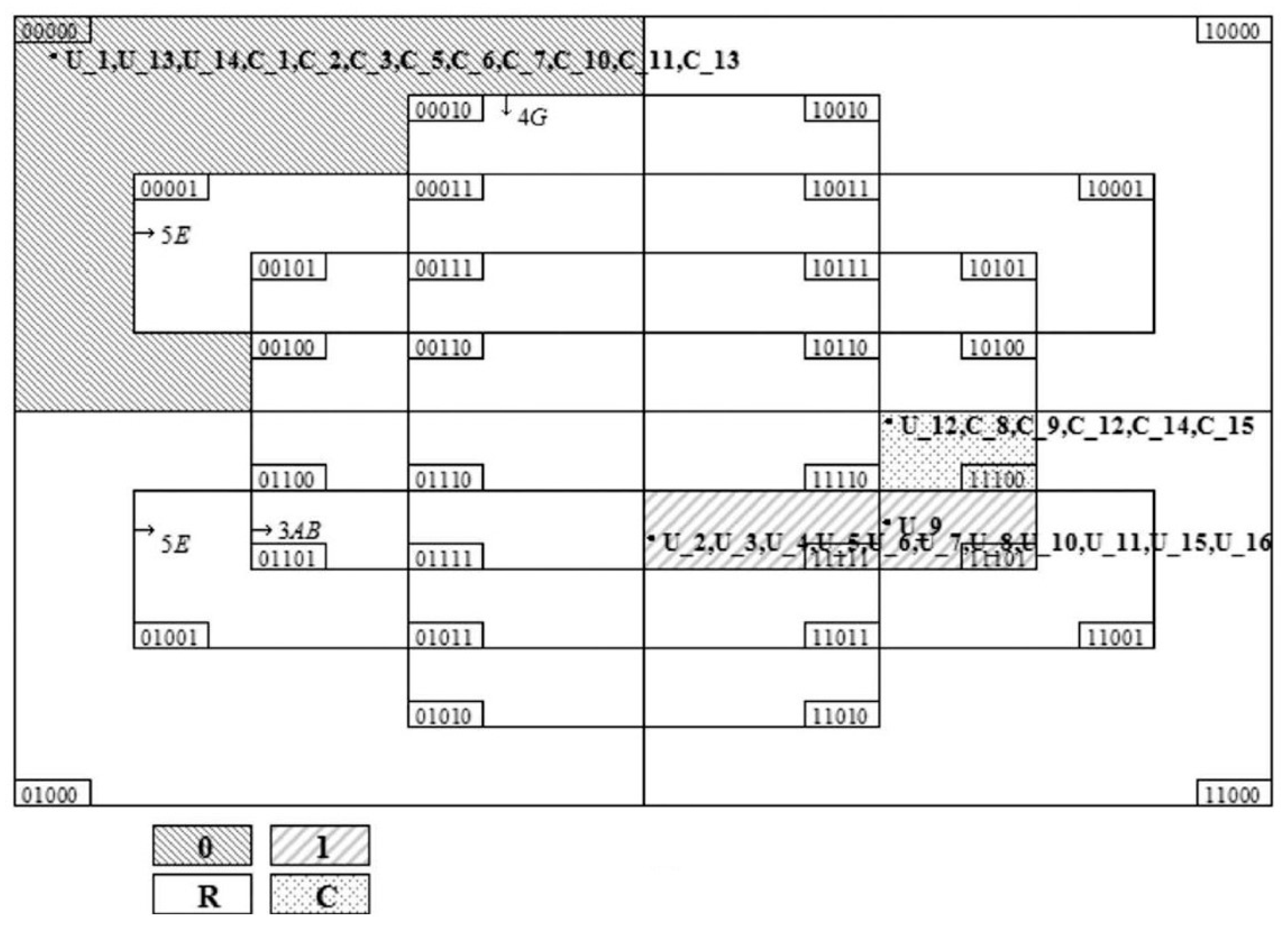
Results from the QCA method (see Figure 1) can be used to study whether empirical data from the assessment of mathematical skills are manifested (or not manifested). Students in the activity group were designated by the prefix U. Students in the control group were designated by the prefix C. A positive learning outcome is represented by a (1) if it is observed in the student’s artifact, and (0) denotes the absence of a desired learning outcome. In the values for (ARTIFACT OUTCOME): (1) signified that the student was successful in producing an artifact that could demonstrate the desired learning outcome, whereas (0) signified that the student was unsuccessful in producing an artifact that could demonstrate the desired learning outcome. For instance, as an extreme example to illustrate how QCA works, if a student is in the area represented as 11110 in the QCA Venn diagram, it means that a particular student has scored full marks for the four questions in a mathematics worksheet, but the student has not managed to produce a hands-on class project that demonstrates the full ability to utilize those mathematical concepts to achieve a passing grade.

The results of a QCA Venn diagram (such as Figure 1) can be used to represent the four types of learning outcomes. A good result (1) is one in which the student’s artifact demonstrates a favorable learning outcome. A negative outcome (0) indicates that the student’s artifact did not demonstrate the desired learning outcome. Contradictory configurations C may develop when certain combinations of factors provide a (0) negative outcome while others produce a (1) good outcome. At first glance, it may appear as though negative cases (0) and contradictory cases C are undesirable outcomes of the QCA approach; however, conflicting configurations can be viewed as results in and of themselves, since they allow the researcher to interact more deeply with the data. For instance, this could mean that, while the student’s artifact did not accomplish the desired learning goal, observable evidence of specific competencies was present in the student’s artifact. Logical remainders R are denoted by blank white spaces to represent unobserved logical conditions.

The educational implication is that QCA can be used to inform the teachers about which specific student to focus on to provide remediation, so that any confusion in the mathematical concepts can be clarified for those students. Students who performed well in both the worksheets and in producing the final project can be encouraged to provide peer-teaching and support to the lower progress students who experienced difficulties.

5. Discussion

Many researchers and educators acknowledge the importance of preparing students for the future [18]. Mathematics education is the must-have core foundation for accessing the many other scientific disciplines that are essential for harnessing quantum technologies. There is a wide range of theories on how to teach quantum theory, but little research into which methods work best. More research regarding students’ difficulties, teaching methods, activities, and research tools for a conceptual approach to quantum mechanics is needed.

Bitzenbauer [19] has shown that quantum physics education research output has increased steadily during the last two decades. In addition, there has been a shift in research priorities. There has been an increase recently in the relevance of empirical research on the teaching and learning of quantum physics, whereas before only publications on the teaching of quantum physics content were published.

Murina [20] observes that we are witnessing a quantum computing revolution that will be vital to the future worldwide dominance of nations. Devices and breakthroughs in the field of quantum physics have been achieved. Quantum computing and technology, as well as fields such as science, technology, engineering, and mathematics, must be taught to the general public. For the development of high-quality quantum technology, a workforce must have a strong foundation in math. In order to enter the field of quantum programming, one must have a solid foundation in arithmetic and physics, both of which are required for quantum literacy.

The majority of quantum information science and technology (QIST) teaching and training takes place at the graduate and postdoctoral levels, with only a few initiatives beginning at the undergraduate level. Expanding these efforts at the pre-tertiary school level and including quantum information science in the curriculum are essential if we are to fulfill the anticipated demand for quantum workers and ensuring that the workforce is demographically representative and includes people from all communities [21].

By utilizing the quantum rules of nature, quantum computing is able to create algorithms that are not achievable on more standard computers, which could lead to significant advances in fields such as materials science and chemistry. Quantum programmers, in particular, are in high demand due to the burgeoning field of quantum computing. Few options exist for non-specialists or knowledge on how to best instruct students in computer science and engineering. Using a realistic, software-driven approach, Mykhailova and Svore [22] taught an undergraduate course on quantum computing. Hands-on programming exercises, several programming assignments, and a final project are all used to supplement lectures on quantum algorithms. Instead of standard written assignments, the emphasis is placed on self-paced programming exercises called “Quantum Katas”. Programming assignments were found to aid students in retaining the theoretical concepts provided in lectures. Students said that the programming exercises and the final project were the most important parts of their learning experience.

Despite the fact that quantum computers and simulators may already be accessed and programmed via the internet, efforts to increase awareness of quantum computing are just getting underway. Angara, Stege, and MacLean [23] described their experiences in arranging and presenting quantum computing seminars for high-school students with little or no prior knowledge in the aforementioned domains. Quantum computing is introduced to students in novel ways, such as through newly created “unplugged” exercises for teaching basic quantum computing ideas. They use a programmatic approach and introduce students to the IBM Q Experience using Qiskit and Jupyter notebooks. Students’ experiences and findings show that basic quantum computing ideas are accessible to high-school students, and early exposure to quantum computing is a desirable addition to the problem-solving and computing abilities that high-schoolers learn before entering university.

Research on how to teach quantum mechanics at the secondary and lower undergraduate levels has been investigated by Krijtenburg-Lewerissa, Brinkman, and van Joolingen [24]. Quantum mechanics is increasingly being taught using a conceptual approach in introductory physics courses around the world. It is necessary to do research on common misunderstandings about quantum mechanics, as well as to conduct tests and develop teaching strategies. For secondary and lower undergraduate students, little research has been done on teaching sophisticated quantum phenomena such as time dependence, superposition, and measurement issues.

It was shown by Rasa, Palmgren, and Laherto [25] that upper-secondary school students’ conceptions of the future and their agentic orientations changed after taking a course on quantum computing and technical approaches to global problems. The researchers found that students had a more positive, yet unpredictable, view of the future and technological development. They also found that students had a more positive view of their own agency and a more positive outlook on the future. A course that focuses on futuristic technologies can help students to think more imaginatively about their own lives, as well as technology and non-technological solutions to global challenges, and to question deterministic thinking. Futuristic quantum physics have opened fresh perspectives on uncertainty and probabilistic reasoning, respectively. A future-oriented approach to teaching science addresses the need of combining future-thinking abilities, student autonomy and real socio-scientific challenges.

Quantum physics education for K12 students and the broader public has become an unavoidable necessity in light of the impending transformative power of quantum technologies. Quantum literacy is crucial for individuals to learn how to foster creativity and develop a new style of thinking. In scientific reasoning, facts and knowledge are analyzed, and then expressed using mathematical language. Foti, Anttila, Maniscalo, and Chiofalo [26] suggest that mathematical frameworks can be used to help students grasp the concepts.

At both the high school and college levels, teaching and mastering quantum mechanics is a challenging endeavor. Students must cope with notions such as uncertainty and entanglement, as well as advanced mathematical tools, in order to fully grasp the new physical world. As a simple solution to these crucial challenges, a matrix algebra-based mathematical approach is offered by Di Mauro and Naddeo [27]. They assert that, to close the gap between high school curricula and contemporary scientific concepts, students can benefit by learning topics such as qubits and quantum computing.

6. Conclusions

Mathematics has long been perceived as difficult by many people. Despite this, mathematics is a vital part of STEM education. Industrial sectors, such as banking, aeronautics, and energy, have already reaped the benefits of quantum technology, and this impact will only grow in more sectors in the future. Managers in the private and public sectors will have to master quantum computing. A better knowledge of quantum algorithms might help foster a greater interest in mathematics. In order to get people excited about the mathematics they already know, the current article suggests presenting the material in a gentle yet understandable manner. The mathematics needed to describe quantum computing concepts, such as linear transformations and matrix algebra, has been introduced. Basic mathematical ideas have been utilized as examples to demonstrate the applicability of these principles in designing algorithms for quantum entanglement, quantum cryptography, and quantum teleportation. These quantum algorithmic literacy exemplars may help rekindle interest in mathematics.

Quantum algorithmic literacy must be taught to the next generation of application domain specialists as well as to a far larger portion of the present workforce. Quantum algorithmic literacy may be used to frame educational endeavors. People who are conversant in both professions would be in high demand. As quantum computing becomes a viable technology, a deeper grasp of the possible uses of quantum computing algorithms would contribute to healthcare, education, government, and other fields. Quantum technology has the potential to revolutionize a wide range of industries. Readers who have already familiar with the basic quantum algorithms introduced in this paper may be interested in more advanced quantum machine learning algorithms such as Grover search and Shor’s algorithm. Many additional algorithms with demonstrable improvements have been created based on these and other discoveries, with applications in fields such as optimization and cryptography. Having a working knowledge of the mathematics needed to craft quantum algorithms would help more people in a variety of professions to innovate for the betterment of humanity.

References

- Perdomo-Ortiz, A.; Feldman, A.; Ozaeta, A.; Isakov, S.V.; Zhu, Z.; O’Gorman, B.; Katzgraber, H.G.; Diedrich, A.; Neven, H.; de Kleer, J.; et al. Readiness of Quantum Optimization Machines for Industrial Applications. Phys. Rev. Appl. 2019, 12, 014004. [Google Scholar] [CrossRef] [Green Version]
- Rainò, G.; Novotny, L.; Frimmer, M. Quantum Engineers in High Demand. Nat. Mater. 2021, 20, 1449. [Google Scholar] [CrossRef] [PubMed]
- Hadorn, G.H.; Hoffmann-Riem, H.; Biber-Klemm, S.; Grossenbacher-Mansuy, W.; Joye, D.; Pohl, C.; Wiesmann, U.; Zemp, E. (Eds.) Handbook of Transdisciplinary Research; Springer: Dordrecht, The Netherlands, 2008; ISBN 978-1-4020-6698-6. [Google Scholar]
- Nita, L.; Mazzoli Smith, L.; Chancellor, N.; Cramman, H. The Challenge and Opportunities of Quantum Literacy for Future Education and Transdisciplinary Problem-Solving. Res. Sci. Technol. Educ. 2021, 1–17. [Google Scholar] [CrossRef]
- Yates, L.; Millar, V. ‘Powerful Knowledge’ Curriculum Theories and the Case of Physics. Curric. J. 2016, 27, 298–312. [Google Scholar] [CrossRef]
- Dirac, P.A.M. The Quantum Theory of the Electron. Proc. R. Soc. Lond. A 1928, 117, 610–624. [Google Scholar] [CrossRef] [Green Version]
- Manin, Y.I. Quantum Groups and Noncommutative Geometry; CRM Short Courses; Springer International Publishing: Cham, Switzerland, 2018; ISBN 978-3-319-97986-1. [Google Scholar]
- Benioff, P. Quantum Mechanical Hamiltonian Models of Turing Machines. J. Stat. Phys. 1982, 29, 515–546. [Google Scholar] [CrossRef]
- Feynman, R.P. Quantum Mechanical Computers. Opt. News 1985, 11, 11. [Google Scholar] [CrossRef]
- Zeh, H.D. On the Interpretation of Measurement in Quantum Theory. Found. Phys. 1970, 1, 69–76. [Google Scholar] [CrossRef]
- Feit, M.D.; Fleck, J.A.; Steiger, A. Solution of the Schrödinger Equation by a Spectral Method. J. Comput. Phys. 1982, 47, 412–433. [Google Scholar] [CrossRef]
- Descartes, R. Descartes: Selected Philosophical Writings, 1st ed.; Cottingham, J., Stoothoff, R., Murdoch, D., Kenny, A., Eds.; Cambridge University Press: Cambridge, UK, 1988; ISBN 978-0-521-35264-2. [Google Scholar]
- Horodecki, R.; Horodecki, P.; Horodecki, M.; Horodecki, K. Quantum Entanglement. Rev. Mod. Phys. 2009, 81, 865–942. [Google Scholar] [CrossRef] [Green Version]
- Hughes, R.J.; Alde, D.M.; Dyer, P.; Luther, G.G.; Morgan, G.L.; Schauer, M. Quantum Cryptography. Contemp. Phys. 1995, 36, 149–163. [Google Scholar] [CrossRef] [Green Version]
- Pirandola, S.; Eisert, J.; Weedbrook, C.; Furusawa, A.; Braunstein, S.L. Advances in Quantum Teleportation. Nat. Photon 2015, 9, 641–652. [Google Scholar] [CrossRef]
- Mityushev, V.; Nawalaniec, W.; Rylko, N. Introduction to Mathematical Modeling and Computer Simulations, 1st ed.; Chapman and Hall/CRC: London, UK, 2018; ISBN 978-1-315-27724-0. [Google Scholar]
- Marx, A.; Rihoux, B.; Ragin, C. The Origins, Development, and Application of Qualitative Comparative Analysis: The First 25 Years. Eur. Pol. Sci. Rev. 2014, 6, 115–142. [Google Scholar] [CrossRef] [Green Version]
- Szabo, Z.K.; Körtesi, P.; Guncaga, J.; Szabo, D.; Neag, R. Examples of Problem-Solving Strategies in Mathematics Education Supporting the Sustainability of 21st-Century Skills. Sustainability 2020, 12, 10113. [Google Scholar] [CrossRef]
- Bitzenbauer, P. Quantum Physics Education Research over the Last Two Decades: A Bibliometric Analysis. Educ. Sci. 2021, 11, 699. [Google Scholar] [CrossRef]
- Murina, E. Math and Physics Tools for Quality Quantum Programming. In Quality of Information and Communications Technology; Shepperd, M., Brito e Abreu, F., Rodrigues da Silva, A., Pérez-Castillo, R., Eds.; Communications in Computer and Information Science; Springer International Publishing: Cham, Switzerland, 2020; Volume 1266, pp. 263–273. ISBN 978-3-030-58792-5. [Google Scholar]
- Perron, J.K.; DeLeone, C.; Sharif, S.; Carter, T.; Grossman, J.M.; Passante, G.; Sack, J. Quantum Undergraduate Education and Scientific Training. arXiv 2021, arXiv:2109.13850. [Google Scholar] [CrossRef]
- Mykhailova, M.; Svore, K.M. Teaching Quantum Computing through a Practical Software-Driven Approach: Experience Report. In Proceedings of the 51st ACM Technical Symposium on Computer Science Education, Portland, OR, USA, 26 February 2020; ACM: New York, NY, USA, 2020; pp. 1019–1025. [Google Scholar]
- Angara, P.P.; Stege, U.; MacLean, A. Quantum Computing for High-School Students An Experience Report. In Proceedings of the 2020 IEEE International Conference on Quantum Computing and Engineering (QCE), Denver, CO, USA, 12–16 October 2020; IEEE: Piscataway, NJ, USA, 2020; pp. 323–329. [Google Scholar]
- Krijtenburg-Lewerissa, K.; Pol, H.J.; Brinkman, A.; van Joolingen, W.R. Insights into Teaching Quantum Mechanics in Secondary and Lower Undergraduate Education. Phys. Rev. Phys. Educ. Res. 2017, 13, 010109. [Google Scholar] [CrossRef] [Green Version]
- Rasa, T.; Palmgren, E.; Laherto, A. Futurising Science Education: Students’ Experiences from a Course on Futures Thinking and Quantum Computing. Instr. Sci. 2022, 1–23. [Google Scholar] [CrossRef]
- Foti, C.; Anttila, D.; Maniscalco, S.; Chiofalo, M. Quantum Physics Literacy Aimed at K12 and the General Public. Universe 2021, 7, 86. [Google Scholar] [CrossRef]
- Di Mauro, M.; Naddeo, A. Introducing Quantum Mechanics in High Schools: A Proposal Based on Heisenberg’s Umdeutung. In Proceedings of the 1st Electronic Conference on Universe, Online, 22 February 2021; MDPI: Basel, Switzerland, 2021; p. 8. [Google Scholar]
Figure 1.
Venn diagram of the QCA results of empirical data in the students (e.g., C_1, C_2, etc.) from the control group compared to the students (U_1, U_2, etc.) from the activity group.
Publisher’s Note: MDPI stays neutral with regard to jurisdictional claims in published maps and institutional affiliations. |
© 2022 by the author. Licensee MDPI, Basel, Switzerland. This article is an open access article distributed under the terms and conditions of the Creative Commons Attribution (CC BY) license (https://creativecommons.org/licenses/by/4.0/).
Share and Cite
MDPI and ACS Style
How, M.-L. Advancing Multidisciplinary STEM Education with Mathematics for Future-Ready Quantum Algorithmic Literacy. Mathematics 2022, 10, 1146. https://0-doi-org.brum.beds.ac.uk/10.3390/math10071146
AMA Style
How M-L. Advancing Multidisciplinary STEM Education with Mathematics for Future-Ready Quantum Algorithmic Literacy. Mathematics. 2022; 10(7):1146. https://0-doi-org.brum.beds.ac.uk/10.3390/math10071146
Chicago/Turabian StyleHow, Meng-Leong. 2022. "Advancing Multidisciplinary STEM Education with Mathematics for Future-Ready Quantum Algorithmic Literacy" Mathematics 10, no. 7: 1146. https://0-doi-org.brum.beds.ac.uk/10.3390/math10071146
Note that from the first issue of 2016, this journal uses article numbers instead of page numbers. See further details here.