Coherence Coefficient for Official Statistics

Abstract

One of the quality requirements in official statistics is coherence of statistical information across domains, in time, in national accounts, and internally. However, no measure of its strength is used. The concept of coherence is also met in signal processing, wave physics, and time series. In the current article, the definition of the coherence coefficient for a weakly stationary time series is recalled and discussed. The coherence coefficient is a correlation coefficient between two indicators in time indexed by the same frequency components of their Fourier transforms and shows a degree of synchronicity between the time series for each frequency. The usage of this coefficient is illustrated through the coherence and Granger causality analysis of a collection of numerical economic and social statistical indicators. The coherence coefficient matrix-based non-metric multidimensional scaling for visualization of the time series in the frequency domain is a newly suggested method. The aim of this article is to propose the use of this coherence coefficient and its applications in official statistics.

1. Introduction

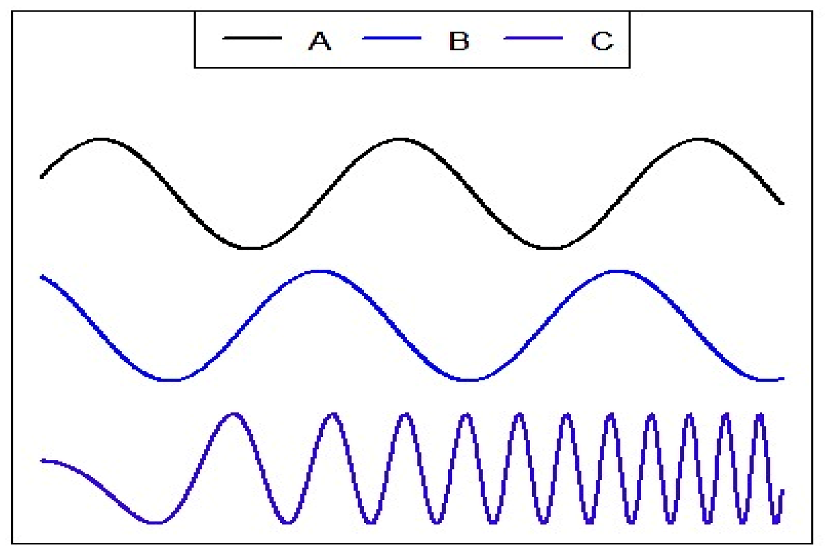
Signals are information carriers; a speech signal delivers semantic meanings, traffic signals give instructions or directions, brain signals reflect the intent of the subject, etc. Signals are often converted to other signals through a certain conversion system. When an input signal is applied, we cannot observe the response associated with that input; we are always faced with a certain amount of additional noise on the output. The relationship between two signals is measured by the coherence coefficient, which is defined as a cross-spectral density between these signals divided by the product of auto-spectral densities of each of them. It can be viewed as a squared correlation between Fourier transformation components of these signals at the same frequency [1,2]. The coherence coefficient gets a value of 1 in the case of a perfect linear relationship between the Fourier components, and a value of 0 for no linear relationship and all values in between [3]. If a small stone is dropped on a still water surface, we see waves of the same length and periodicity. It is said in wave physics that two waves are coherent if they have the same permanent wave length and frequency and their phase difference is constant [4]. For example, waves A and B in Figure 1 are coherent, but none of them is coherent with wave C, which has a different changeable frequency.

Coherent sources of light are sources of light that emit waves which have zero or constant phase difference and same the frequency. Incoherent sources are sources of light that emit waves which have random frequencies and phase differences. The coherence coefficient gives an answer when measuring the degree of coherence of light waves and signal input/output.

The concept of coherence is used in many fields of science, official statistics being one of them. As stated in Principle 14 of the European Statistics Code of Practice [5], official “statistics are internally coherent and consistent”. Consistency means validity of the arithmetic and accounting identities. At first sight, it looks like this meaning of coherence is completely different from the concept of coherence used in physics. In this paper, we will try to reveal similarities in these two understandings and propose to include a numerical measure of coherence to official statistics. Let us look at how different institutions understand coherence. According to the OECD Glossary [6], coherence of statistics is their suitability to be reliably combined for various aims and in different ways. Statistics may originate from a single source. In that case, their coherence means the possibility to combine elementary concepts correctly in more complex ways and for various aims. Statistics may originate from different sources and from statistical surveys of different frequencies. In that case, their coherence means the usage of common definitions, classifications and methodological principles. Consistency is understood simply as a separate aspect of coherence.

The Statistics Canada Quality Guidelines [7] state that coherence of statistical information means the degree to which it can be reliably aggregated and compared with other statistical information by methodological principles and over time. How should this degree be measured? The quality indicators for coherence are proposed in this document as adequacy to the “regional and international standards for statistical methods” and the reasons why some effects in statistical information cannot be fully explained by accuracy are listed. As we see, it is proposed to describe coherence only verbaly, and no numerical measure for the “degree to which statistical information can be reliably combined” is proposed.

The Australian Bureau of Statistics affirms that coherence refers to the internal consistency of data at a fixed time point and over time, and to its comparability with other sources of information [8].

Various aspects of coherence are presented and discussed in the Eurostat’s Handbook for Quality Reports [9] including coherence across domain, in sub-annual and annual statistics, in national accounts, as well as internal coherence. The Handbook mentions that preferably, a quantitative assessment of the possible effects in the statistical output results should be included in the statistical Quality Report. However, no coherence measures are proposed. From this we can see that, in official statistics, coherence is mainly about outputs.

It is felt that coherence in official statistics means similar trends in the indicator, and can therefore be compared with the waving situation in physics. At the same time, there is an observable difference between the concept of coherence in wave physics and in official statistics. Nevertheless, there is a clearly observable aspiration in official statistical documentation to measure the degree of coherence, even if it is not known how to do it yet. Indeed, there have been attempts, found in the official statistics literature, to measure coherence numerically.

The contents of the article are as follows. Section 2 includes an overview of the studies in the quantitative assessment of coherence in official statistics. The definition of the coherence coefficient is restated in Section 3. The fields of its application—time series causality and non-metric multidimensional scaling—are also presented in Section 3. The application of these methods for economic and social time series is given in Section 4. The article ends with conclusions and a list of references. The dataset used is presented in the

Table A1. Data set for the case study [37].

Year	Quarter	ExU	LFSU	LFSE	Emp	RSI	RRS	REM
2008	1	76,247	74.2	1416.3	1,225,579	623.1	2,308,808,359	2,363,109,444
2008	2	68,377	68.5	1432.1	1,225,139	647.8	2,406,414,174	2,461,320,556
2008	3	69,056	90.2	1445.8	1,217,387	671.9	2,461,575,844	2,519,700,890
2008	4	79,839	120.2	1414.2	1,182,155	671.7	2,344,094,370	2,448,874,661
2009	1	150,867	183.4	1329.9	1,153,522	635.2	2,133,829,174	2,184,921,227
2009	2	193,005	210.9	1321.6	1,105,870	629.2	2,022,994,119	2,066,057,345
2009	3	216,797	211.8	1329.8	1,069,554	620.4	1,920,387,308	1,973,800,770
2009	4	251,803	236.5	1288.3	1,035,599	613.5	1,820,404,831	1,869,016,244
2010	1	298,039	272.2	1221.9	1,029,803	588.3	1,727,789,493	1,774,727,272
2010	2	324,468	273.7	1231.0	1,031,499	595.4	1,772,024558	1,819,986,665
2010	3	319,943	270.5	1261.5	1,038,689	602.9	1,818,575,281	1,860,114,000
2010	4	306,016	265.3	1276.2	1,037,375	614.4	1,861,967,661	1,905,767,899
2011	1	303,692	255.1	1232.9	1,059,600	600.0	1,840,842,491	1,871,739,022
2011	2	246,707	232.9	1262.2	1,080,333	610.4	1,938,042,383	1,975,212,406
2011	3	221,274	221.3	1260.7	1,094,869	612.8	1,982,452,866	2,024,025,178
2011	4	217,134	202.8	1258.7	1,090,185	629.9	2,025,371,521	2,072,390,439
2012	1	242,059	212.7	1251.4	1,101,293	619.2	1,985,074,588	2,025,141,063
2012	2	216,475	196.5	1284.1	1,113,460	623.7	2,046,589,574	2,091,059,274
2012	3	205,422	185.5	1298.0	1,117,600	628.8	2,078,963,346	2,128,180,667
2012	4	203,537	192.5	1269.4	1,110,714	646.4	2,124,877,617	2,173,804,073
2013	1	229,502	191.2	1267.2	1,126,036	646.7	2,122,599,794	2,165,028,897
2013	2	197,661	171.8	1297.1	1,138,652	652.5	2,196,084,239	2,252,422,898
2013	3	185,739	159.6	1308.2	1,147,276	667.7	2,265,256,537	2,321,432,196
2013	4	192,387	167.2	1298.6	1,140,335	677.8	2,278,247,315	2,327,255,164
2014	1	206,079	183.4	1295.3	1,161,133	670.7	2,264,769,393	2,309,649,474
2014	2	167,988	165.5	1309.2	1,175,198	682.3	2,353,632,663	2,402,902,573
2014	3	157,944	135.4	1349.2	1,177,126	696.7	2,401,668,920	2,446,552,234
2014	4	160,011	147.8	1322.4	1,169,402	714.5	2,448,904,478	2,493,322,593
2015	1	171,767	145.8	1317.5	1,194,723	699.8	2,424,880,432	2,473,235,328
2015	2	154,516	138.0	1336.3	1,204,611	713.9	2,524,677,556	2,586,979,303
2015	3	151,583	122.5	1347.4	1,204,198	735.1	2,606,122,113	2,669,476,792
2015	4	154,745	129.5	1338.5	1,194,923	756.9	2,655,432,571	2,716,650,174
2016	1	165,882	122.5	1350.8	1,210,243	748.0	2,635,907,896	2,687,204,050
2016	2	139,980	119.1	1367.7	1,219,175	771.9	2,766,639,327	2,821,945,721
2016	3	134,454	111.0	1368.7	1,217,086	793.3	2,857,993,212	2,911,196,395
2016	4	139,141	112.0	1358.4	1,210,342	822.8	2,937,353,990	2,994,475,146
2017	1	153,495	117.7	1345.3	1,222,378	817.6	2,900,763,204	2,957,958,651
2017	2	133,083	102.2	1362.8	1,230,629	838.7	3,045,375,323	3,129,433,254
2017	3	132,574	95.5	1358.8	1,226,833	850.8	3,092,979,211	3,164,580,713
2017	4	139,308	97.1	1352.3	1,222,817	884.8	3,190,590,164	3,269,956,131
2018	1	162,200	103.9	1347.1	1,230,548	895.2	3,212,311,031	3,273,567,722
2018	2	143,082	86.0	1370.9	1,235,994	926.7	3,408,966,239	3,481,541,119
2018	3	144,222	82.9	1404.9	1,237,430	935.7	3,460,961,589	3,537,412,644
2018	4	154,430	87.4	1376.0	1,234,872	970.3	3,561,459,073	3,647,635,020
2019	1	155,921	95.1	1374.0	1,250,723	1262.7	3,601,427,871	3,671,909,464
2019	2	138,469	90.2	1382.2	1,260,340	1289.0	3,757,034,213	3,858,893,280
2019	3	137,013	88.9	1378.1	1,260,575	1317.6	3,847,743,644	3,940,044,105
2019	4	150,469	93.7	1379.4	1,256,362	1358.6	3,941,919,691	4,036,791,146
2020	1	169,436	106.3	1386.4	1,271,002	1381.0	3,995,577,232	4,074,616,070
2020	2	208,074	125.9	1351.5	1,245,638	1398.5	3,867,650,330	3,964,444,596
2020	3	243,271	137.2	1342.3	1,244,455	1454.8	4,172,921,127	4,268,937,946
2020	4	277,119	134.5	1352.4	1,248,681	1524.2	4,357,386,170	4,436,727,466
2021	1	259,800	108.8	1351.8	1,263,441	1517.4	4,363,643,377	4,448,379,003

.

The concept of the coherence coefficient was included by the author in the Final Report of the project Komuso [10] and Workshop paper [11].

2. Literature Overview of the Coherence Assessment in Official Statistics

The coherence of statistics across programmes has been investigated in several studies. Till-Tentschert [12] discusses the coherence assessment in the European Union Statistics on Income and Living Conditions (EU-SILC) at Statistics Austria. The distribution of annual gross employee income according to the EU-SILC 2005 and wage tax statistics 2004 are compared using their distributions by percentile. A conclusion is made about the high coherence (visually) for the number of income recipients. Comments are made about the difference of these distributions. One of the important conclusions is that coherence assessment stimulates critical quality assessment. As regards said paper, we would like to remark that the statistical hypothesis about the coincidence of two distributions can be tested by means of statistical test in order to get a more reliable conclusion on coherence (for example, by means of a two-sample Kolmogorov–Smirnov test).

Three examples are given for reconciling the Labour Force Survey (LFS) data with national accounts, with the results of industrial surveys of large establishments, and with administrative data on registered job seekers by the African Development Bank [13]. The essence of these examples is the decomposition of the coverage of the indicators into subsets with the aim to find the same subset covered by both indicators, the same definitions of the variables used, and to compare their values. The differences are expected to depend only on random fluctuations. It is shown in the document that the trends in employment and production follow the same pattern. If, according to LFS, employment increases, then an increase in production is expected in the national accounts. Correspondingly, if the LFS results show a decline in the level of employment, it should be followed by a decline in the level of production in the national accounts. This consideration reveals a comparison of the trends in the time series.

The population size in population statistics and the population size estimates based on the data from the European Union LFS (EU-LFS) usually differ due to the different coverage (EU-LFS covers only private households). Both statistics refer to certain dates: population statistics refer to January 1 or mid-year for the population level and characteristics, and the EU-LFS statistics generally refer to the average quarterly or annual situation. 15–64-year-old population size levels and their relative differences in two different datasets by country are presented by Eurostat [14].

The differences in employment statistics in the EU-LFS and business statistics are discussed in three aspects: different scope, different coverage, and different units. Levels, their differences and relative differences by country are presented by Eurostat [14].

3. Coherence of the Time Series

Wiener, 1930 [15], starts his article emphasising the close analogy between the problems of the harmonic analysis of light and the hidden periods found by the statistical analysis in the data sets such as of meteorology and astronomy. He pays attention to the “extremely valuable theory of the periodogram”. He subsequently points out the usefulness of the correlation matrices for statistical analysis and the need for statistical methods to study the time series. Finally, Wiener comes to a conclusion that the role of coherence matrices for the time series should be the same as the role of correlation matrices for frequency series. In his paper, he introduced the coherence coefficient of the time series, and we will follow this path, applying the methods proposed in Shumway and Stoffer [16], and Wei [17].

3.1. Stationary Time Series

Let us consider a real-valued time series $x_1,x_2,\dots ,x_n$. It is called a weakly stationary time series if $x_t$ is a finite variance process such that its mean value function ${\mu }_t=\mathbf{E}{x}_t$ is constant and does not depend on time t, and its covariance function, ${\gamma }_x\left(s,t\right)=\mathbf{E}\left[\left(x_t-\mu \right)\left(x_s-\mu \right)\right]$, $s$, $t>0$, depends on $s$ and t only through their difference $h=\left|s-t\right|$, and is denoted by ${\gamma }_x\left(h\right)={\gamma }_x\left(t+h,t\right)$. A covariance of a weakly stationary time series does not depend on time. Henceforth, we will further use the term stationary to mean weak stationarity. It can be observed that $Var\left(x_t\right)={\gamma }_x\left(0\right)$.

A discrete Fourier transform for the time series $x_1,x_2,\dots ,x_n$ is defined as

$$d({\omega }_j)=\frac{1}{\sqrt{n}}{\displaystyle \sum _{t=1}^n{x}_t{e}^{-2\pi i{\omega }_{j}t}}=\frac{1}{\sqrt{n}}{\displaystyle \sum _{t=1}^n{x}_t\left(\cos (2\pi {\omega }_{j}t)-i\sin (2\pi {\omega }_{j}t)\right)}$$

(1)

for $j=0,1,2,\dots ,n-1$ and $i=\sqrt{-1}$ ([16] p. 69). Frequencies ${\omega }_j=j/n$ are called Fourier frequencies, or fundamental frequencies. This transformation is one-to-one, and the inverse discrete Fourier transform allows to express the time series as

$$x_t=\frac{1}{\sqrt{n}}{\displaystyle \sum }_{j=0}^{n-1}d\left({\omega }_j\right)e^{2\pi i{\omega }_{j}t}, t=1,2,\dots ,n.$$

(2)

The inverse Fourier transform expresses stationary time series as a sum of n periodic components which are not observable directly. Periodic components have unequal amplitudes, and the component with a higher amplitude $\left|d({\omega }_j)\right|$ plays a greater role in the Fourier transform.

The periodogram for time series $x_1,x_2,\dots ,x_n$ is defined as a squared modulus of the Fourier transform:

$$I\left({\omega }_j\right)={\left|d\left({\omega }_j\right)\right|}^2, j=0,1,2,\dots ,n-1.$$

The periodogram allows us to compare the role of each component in the transform. We will use it in the next section. The scaled periodogram is

$$P\left(j/n\right)=\frac{4}{n}I\left({\omega }_j\right)=\frac{1}{n}{\left|2d\left({\omega }_j\right)\right|}^2,$$

(Ref. [16], p. 70, (2.46) formula), $j=0,1,2,\dots ,n-1$. It is proven in Shumway [16], that if $x_t$ is stationary with the auto-covariance function $\gamma \left(h\right)=E\left[(x_{t+h}-\mu )(x_t-\mu )\right]$, then there exists a unique monotonically increasing function $F\left(\omega \right)$, called a spectral distribution function, which is bounded, with $F\left(-\infty \right)=F\left(-1/2\right)=0$, and $F(\infty )=F\left(1/2\right)=\gamma \left(0\right)$ such that

$$\gamma \left(h\right)={\int }_{-1/2}^{1/2}{e}^{2\pi i\omega h}dF\left(\omega \right).$$

A more important situation we use repeatedly is the one covered by Theorem C.3 [16], where it is shown that, subject to absolute sumability of the auto-covariance, the spectral distribution function is absolutely continuous with $dF\left(\omega \right)=f\left(\omega \right)d\omega$. The function $f(\omega )$ is called spectral density function.

3.2. Jointly Stationary Time Series

Two time series $x_t$ and $y_t$ are called jointly stationary if each of them is stationary and their cross-covariance function ${\gamma }_{xy}\left(s,t\right)=E\left[\left(x_s-{\mu }_x\right)\left(y_t-{\mu }_y\right)\right]$ depends only on the time difference $\left|t-s\right|$, and ${\gamma }_{xy}\left(t+h,t\right)={\gamma }_{xy}\left(h\right)$, $t\ge 0$. The cross-correlation function of jointly stationary time series $x_t$ and $y_t$ is defined as

$${\rho }_{xy}\left(h\right)=\begin{array}{cc}\frac{{\gamma }_{xy}\left(h\right)}{\sqrt{{\gamma }_x\left(0\right){\gamma }_y\left(0\right)}},& h>0\end{array}.$$

It has properties: $-1\le {\rho }_{xy}(h)\le 1$, ${\rho }_{xy}(-h)={\rho }_{xy}(h)$.

It is proven in Shumway [16] that, for jointly stationary time series, their cross-covariance function can be expressed as

$${\gamma }_{xy}\left(h\right)=\begin{array}{cc}{\int }_{-1/2}^{1/2}{f}_{xy}\left(\omega \right)e^{2\pi i\omega h}d\omega ,& -\infty <t<\infty \end{array},$$

where the cross-spectrum $f_{xy}\left(\omega \right)$ is defined as the Fourier transform

$$f_{xy}(\omega )=\begin{array}{cc}{\displaystyle \sum _{h=-\infty }^{\infty }{\gamma }_{xy}(h)e^{-2\pi i\omega h},}& -1/2\le \omega \le 1/2\end{array},$$

assuming that the cross-covariance function is absolutely sumable. The cross-spectrum $f_{xy}\left(\omega \right)$ is generally a complex-valued function.

3.3. Coherence Coefficient

For the discrete finite time series $x_1,x_2,\dots ,x_n$ and $y_1,y_2,\dots ,y_n$, we have $\omega =j/n$, $j=0,\pm 1,\dots ,\pm \left[n/2\right]$,

$${\gamma }_{xy}(h)=\begin{array}{cc}\frac{1}{n}{\displaystyle \sum _{j=-\left[n/2\right]}^{\left[n/2\right]}{f}_{xy}(j/n)e^{2\pi ijh/n},}& {\gamma }_{xy}\left(0\right)=\frac{1}{n}\end{array}{\displaystyle \sum _{j=-\left[n/2\right]}^{\left[n/2\right]}{f}_{xy}(j/n)},$$

$$f_{xy}\left(j/n\right)={\displaystyle \sum }_{h=-\left[n/2\right]}^{\left[n/2\right]}{\gamma }_{xy}\left(h\right)e^{-2\pi ijh/n}.$$

We propose the application of the cross-spectrum as a measure of strength of the relationship of two time series in their Fourier transform components.

Definition. The sample coherence coefficient in frequency $\omega$ between two time series $x_t$ and $y_t$ is defined as

$$co{h}_{xy}^2\left(\omega \right)=\frac{{\left|f_{xy}\left(\omega \right)\right|}^2}{f_{xx}\left(\omega \right)f_{yy}\left(\omega \right)}$$

(3)

where $f_{xy}(\omega )$ is the cross-covariance (cross-spectral density) of two time series, and $f_{xx}\left(\omega \right)$, $f_{yy}(\omega )$ are the auto-correlation (power spectral density functions) of $x_t$ and $y_t$, respectively.

It is a square of the correlation coefficient between the ω frequency component of $x_t$ and the ω frequency component of y_t (Wei, [17]). The properties of the coherence coefficient follow the correlation coefficient properties:

• $\left|{\mathit{coh}}_{xy}^2\left(\omega \right)\right|\le 1$
• $\left|{\mathit{coh}}_{xy}^2\left(\omega \right)\right|=1$ means that the time series are perfectly correlated or linearly related at frequency ω;
• $\left|{\mathit{coh}}_{xy}^2\left(\omega \right)\right|=0$ means that the time series are totally uncorrelated at frequency ω;
• ${\mathit{coh}}_{xy}^2\left(\omega \right)={\mathit{coh}}_{yx}^2\left(\omega \right)$ means symmetry in x and y at frequency ω.

Coherence measures the degree of linear dependency of two time series indexed by the same frequency components. If two time series correspond to each other linearly perfectly at a given frequency, the magnitude of coherence is 1 at that frequency. If they are totally linearly unrelated, coherence will be 0 at that frequency. The coefficient (3) is sometimes called “ordinary coherence” [18]; it can be calculated for any arbitrary time series x_t and y_t. Its value indicates how much one time series is linearly related to the other time series at the fixed frequency, and this relationship does not mean any causal relationship.

Much research has been carried out to study the coherence coefficient. Papana [19] analyses connectivity measures in multivariate high dimensional systems and classifies them into two broad groups, namely symmetric and directional measures. Coherence and the Pearson correlation coefficient are assigned to the group of non-directional connectivity measures. An algorithm with the commonness between the cluster members measured by coherence is presented in [20]. It shows much better performance than the other methods compared. Coherence-based time series clustering is also used to study brain connectivity [21]. Foster and Guinzy in [22] wrote that, as an estimate of this parameter, most geophysicists have used the “sample coherence” (as given in (3)). They have found that the “Goodman distribution provides a means of constructing estimates of the true coherence, which are better than the widely used sample coherence”. Generalization of the coherence coefficient is extended to continuous time stationary weakly ergodic random processes [18]. Koopmans [23] has defined the coefficient of coherence for bivariate weakly stationary stochastic processes and “provided a justification for the already common use of the coefficient of coherence as a measure of linear-regression for pairs of correlated, weakly stationary time series”. This directs us to the other root of the coherence research connected with causality.

3.4. Coherence and Causality

Besides the common definition of coherence, we present its property which is included in many research works due to its possibility to measure causality in multivariate models. The basics of this connection is presented in the article by Granger [24]. Let us assume there are two jointly weakly stationary time series $x_t$, y_t, t = 1, 2, …, n, with zero means. The simple causal model is expressed:

$$y_t={\displaystyle \sum }_{j=1}^m{a}_j{y}_{t-j}+{\displaystyle \sum }_{j=1}^m{b}_j{x}_{t-j}+{\eta }_t,$$

(4)

$$x_t={\displaystyle \sum }_{j=1}^m{c}_j{x}_{t-j}+{\displaystyle \sum }_{j=1}^m{d}_j{y}_{t-j}+{\epsilon }_t,$$

(5)

here ${\epsilon }_t$, ${\eta }_t$ are uncorrelated white noise time series with zero means, $Var({\epsilon }_t)={\sigma }_{\epsilon }^2$, $Var({\eta }_t)={\sigma }_{\eta }^2$, $t=1,2,\dots ,n$, $a_j,b_j,c_j,d_j$ are constants, $j=1,2,\dots ,m$, $m$ is a positive integer, usually less than $n$. If at least one coefficient $b_j\ne 0$, $j=1,2,\dots ,m$, then it is said that the time series $x_t$ is a Granger cause for time series y_t, and model (4) is called an unrestricted model. Otherwise, if $b_j=0$ for all $j=1,2,\dots ,m$, then the time series x_t is not the Granger cause for the time series y_t and model (4) is called a restricted model. The same applies to model (5) with the roles of the variables x_t and y_t exchanged. If at least one coefficient $d_j\ne 0$, $j=1,2,\dots ,m$, then it is said that the time series y_t is a Granger cause for time series x_t, and it is not so if all d_j = 0. We see, that the only lags are on the right hand side of Equations (4) and (5). It follows from (4) that if x_t is the Granger cause for the time series y_t, then $y_t$ can be predicted using the past values of x_t. In order to test the existence of the Granger causality between the time series, the F test is used. Under the null hypothesis of no causality, it compares the unrestricted model where y_t is explained by the lags of y_t and lags of x_t with the restricted model where $y_t$ is explained only by lags of $y_t$. The fact that $x_t$ is a Granger cause of $y_t$ is denoted by $x_t\Rightarrow y_t$. The reverse relationship in connection with (5) is also used: $x_t\Leftarrow y_t$. If both these events occur, it is said that there is a feedback relation between the time series $x_t$ and $y_t$.

Let us introduce notations:

$$a=a({\mathrm{e}}^{-i\omega })=\begin{array}{cc}{\displaystyle \sum _{j=1}^m{a}_j{\mathrm{e}}^{-i\omega j},}& b=b({\mathrm{e}}^{-i\omega })={\displaystyle \sum _{j=1}^m{b}_j{\mathrm{e}}^{-i\omega j},}\end{array}$$

$$c=c\left(e^{-i\omega }\right)=\begin{array}{cc}{\displaystyle \sum _{j=1}^m}{c}_j{e}^{-i\omega j},& d=d\left(e^{-i\omega }\right)={\displaystyle \sum _{j=1}^m}{d}_j{e}^{-i\omega j},\end{array}$$

$$\Delta ={\left|\left(1-a\right)\left(1-d\right)-bc\right|}^2.$$

Granger showed [24] that in the case of causality, the cross-spectrum of the time series x_t and y_t can be written as a sum of two components:

$$f_{xy}(\omega )=f_{xy}^{(1)}(\omega )+f_{xy}^{(2)}(\omega ),$$

$$f_{xy}^{\left(1\right)}\left(\omega \right)=\frac{{\sigma }_{\epsilon }^2}{2\Delta \pi }\left(1-d\right)\overline{c}, f_{xy}^{\left(2\right)}\left(\omega \right)=\frac{{\sigma }_{\eta }^2}{2\Delta \pi }\left(1-\overline{a}\right)b.$$

If x_t is not a Granger cause for y_t, then the first of these components equals zero: $f_{xy}^{(1)}(\omega )=0$; and if y_t is not a Granger cause for x_t, then the second component equals zero: $f_{xy}^{\left(2\right)}\left(\omega \right)=0$. If x_t is the Granger cause for $y_t$, then the coherence coefficient is defined as

$$co{h}_{x\to y}\left(\omega \right)=\frac{{\left|f_{xy}^{\left(1\right)}\left(\omega \right)\right|}^2}{f_{xx}\left(\omega \right)f_{yy}\left(\omega \right)} \mathrm{for} x_t\Rightarrow y_t.$$

Its size shows the strength of the Granger causality $x_t\Rightarrow y_t$ against frequency $\omega$ and is called causality coherence. The coefficient $co{h}_{x\leftarrow y}\left(\omega \right)$ for $x_t\Leftarrow y_t$ is defined in the same way. From this it follows that: if $x_t$ is not the Granger cause for y_t and y_t is not the Granger cause for x_t, then the coherence coefficient $co{h}_{xy}(\omega )$ should be zero. For an estimated coherence coefficient, it may not be exactly so. We will apply Granger causality to the economic and social time series in Section 4.3.

Granger causality has many applications in various fields of science. Statistical criteria have been developed to test causality in frequency domains, applied to cointegrated systems, the large sample properties of the test studied [25]. The coherence coefficient and Granger causality were considered in oceanography [26]; long-term coherence statistics reduced the misclassification of forests as urban; short-term coherence statistics reduced the misclassification of low vegetation in forests in [27].

To focus specifically on the temporal dimension of interactions between the brain regions, Granger causality and coherence were used in [28]. Brain functional connectivity was studied in [29].

3.5. Coherence and Multivariate Data Analysis

Correlation matrices are the starting point for many multivariate analysis methods. We observe that a similar situation arises with the ordinary coherence coefficient matrices. In the case of multivariate time series, the principal component analysis is used to reduce dimensionality, and a coherence coefficient matrix is used as a measure of proximity of the relationship between the variables in the frequency domain [30,31]. The canonical correlation analysis may be used to study the association between two signal groups in the frequency domain using coherence coefficients instead of correlation coefficients [32,33]. In this case it would be worth renaming the method as “canonical coherence analysis”. The set of coherence definitions is widened by introducing block coherence, multiple coherence, intra-block coherence, and partial block coherence—to measure the interdependence between multidimensional time series [34].

Along with other coherence matrix-based multivariate time series methods, such as principal component analysis [30,31] and canonical correlation analysis [32,33], a collection of multivariate analysis methods for time series is supplemented here by introducing a new version of a multidimensional scaling method in frequency domain based on the coherence matrix. Multidimensional scaling is a group of methods that project multidimensional data to a low (usually two) dimensional space and preserve the interpoint distances among data as much, as possible.

Let us have number K discrete finite weakly jointly stationary time series $x_1^{(k)},x_2^{(k)},\dots ,x_n^{(k)}$, $k=1,2,\dots ,K$ (or K-dimensional time series) for which the Fourier transforms (2) are defined, the expressions for cross-covariance and cross-spectral density are as follows

$$\begin{array}{cc}{\gamma }_{kl}\left(h\right)=\frac{1}{n}{\displaystyle \sum _{j=-\left[n/2\right]}^{\left[n/2\right]}}{f}_{x^{\left(k\right)}{x}^{\left(l\right)}}\left(j/n\right)e^{2\pi ijh/n},& f_{kl}\left(j/n\right)={\displaystyle \sum _{h=-\left[n/2\right]}^{\left[n/2\right]}}{\gamma }_{kl}\left(h\right)e^{2\pi ijh/n}\end{array},$$

$j=0,\pm 1,\dots ,\pm \left[n/2\right]$, and coherence coefficients for $k,l=1,2,\dots ,K$, are denoted:

$$co{h}_{kl}^2\left(\omega \right)=\frac{{\left|f_{kl}\left(\omega \right)\right|}^2}{f_{kk}\left(\omega \right)f_{ll}\left(\omega \right)}.$$

Coherence matrices are recorded for all frequencies:

$$G(\omega )=\left(\begin{array}{cccc}1& co{h}_{12}^2\left(\omega \right)& \dots & co{h}_{1K}^2\left(\omega \right)\\ co{h}_{21}^2\left(\omega \right)& 1& \dots & co{h}_{2K}^2\left(\omega \right)\\ \dots & \dots & \dots & \dots \\ co{h}_{K1}^2\left(\omega \right)& co{h}_{K2}^2\left(\omega \right)& \dots & 1\end{array}\right).$$

(6)

The aim of multidimensional scaling is to produce a map of time series in the frequency domain, rather directly on the data. A distance matrix or a dissimilarity matrix is used instead. In the case of distance matrix multidimensional scaling is called metric; for this purpose, Euclidean or Manhatan distances may be used. In the case of dissimilarity matrix, multidimensional scaling is called non-metric. The values of the ranking variable matrix may play the role of the dissimilarity matrix. The coherence matrix is a similarity matrix, however, if we extract each of its terms from the unit, we obtain the following dissimilarity matrix:

$$\tilde{G}(\omega )=\left(\begin{array}{cccc}0& 1-co{h}_{12}^2\left(\omega \right)& \dots & 1-co{h}_{1K}^2\left(\omega \right)\\ 1-co{h}_{21}^2\left(\omega \right)& 0& \dots & 1-co{h}_{2K}^2\left(\omega \right)\\ \dots & \dots & \dots & \dots \\ 1-co{h}_{K1}^2\left(\omega \right)& 1-co{h}_{K2}^2\left(\omega \right)& \dots & 0\end{array}\right).$$

Any element of this matrix will be close to zero, if it belongs to the perfectly linearly correlated and synchronised time series components at frequency ω and vice versa: the high value of the matrix $\tilde{G}(\omega )$ element corresponds to unsynchronised time series components.

For the sake of simplicity let us denote the elements of the dissimilarity matrix $\tilde{G}\left(\omega \right)$ by ${\delta }_{kl}$, $k,l=1,2,\dots ,K$. They are symmetric in their indexes: ${\delta }_{kl}={\delta }_{lk}$. Let us fix at the beginning one frequency ω and denote by X the m-dimensional space to which $K$-dimensional time series at frequency ω should be projected. Let $d=d(X)=\left\{\begin{array}{cc}{d}_{kl}(X),& 0<k<l\le K\end{array}\right\}$ be a set of coordinates in the space X to which dissimilarities ${\delta }_{kl}$ are projected (dissimilarities with symmetric indices are not included). The coordinates $d_{kl}=d_{kl}\left(X\right)$ should be chosen in such a way, that the distance (defined in a certain way) between $d_{kl}$ and ${\delta }_{kl}$ is minimal. This is done not directly, but rather converting dissimilarities ${\delta }_{kl}$ into disparities ${\widehat{d}}_{kl}$ by ranking dissimilarities:

$$\mathrm{if} {\delta }_{kl}<{\delta }_{rs} \mathrm{then} {\widehat{d}}_{kl}\le {\widehat{d}}_{rs}, k,l,r,s=1,2,\dots ,K, k<l, r<s$$

A normalized stress function, defined by the equation

$$S_m\left(X\right)=\frac{{\displaystyle \sum _{k<l}}{({\widehat{d}}_{kl}-d_{kl}\left(X\right))}^2}{{\displaystyle \sum _{k<l}}{d}_{kl}^2\left(X\right)}$$

from ref. [35], is used as a criteria to find the solution. The vector of coordinates $\widehat{\mathbf{d}}=\widehat{\mathbf{d}}\left(X\right)=\left\{\begin{array}{cc}{\widehat{d}}_{kl}\left(X\right),& 0<k<l\le K\end{array}\right\}$ which minimises the stress function $S_m(X)$ provides a solution to the multidimensional scaling problem. A certain iterative process is used for the minimization of the stress function. If ${\min }_{d(X)}{S}_m(X)\le 0.05$, then the point of the minimum of the stress function is considered as appropriate. In the case of a two-dimensional space X $(m=2)$ the dissimilarities in the matrix $\tilde{G}\left(\omega \right)$ are projected into the distances on the plane X. So, the multidimensional scaling is a method of visualisation of the time series: by presenting a sequence of multivariate projections of the multivariate time series for subsequent frequencies we are able to observe the change of multivariate time series following the frequency change. The plot of the time series components by points in the X space allows classifying these components for each frequency.

A variety of variants available for multidimensional scaling of variables [36] can be transformed in order to be used for the time series based on the coherence matrix.

4. Experimental Results

4.1. Data Used for the Study

Let us see how the coherence coefficient works for the indicators produced by official statistics.

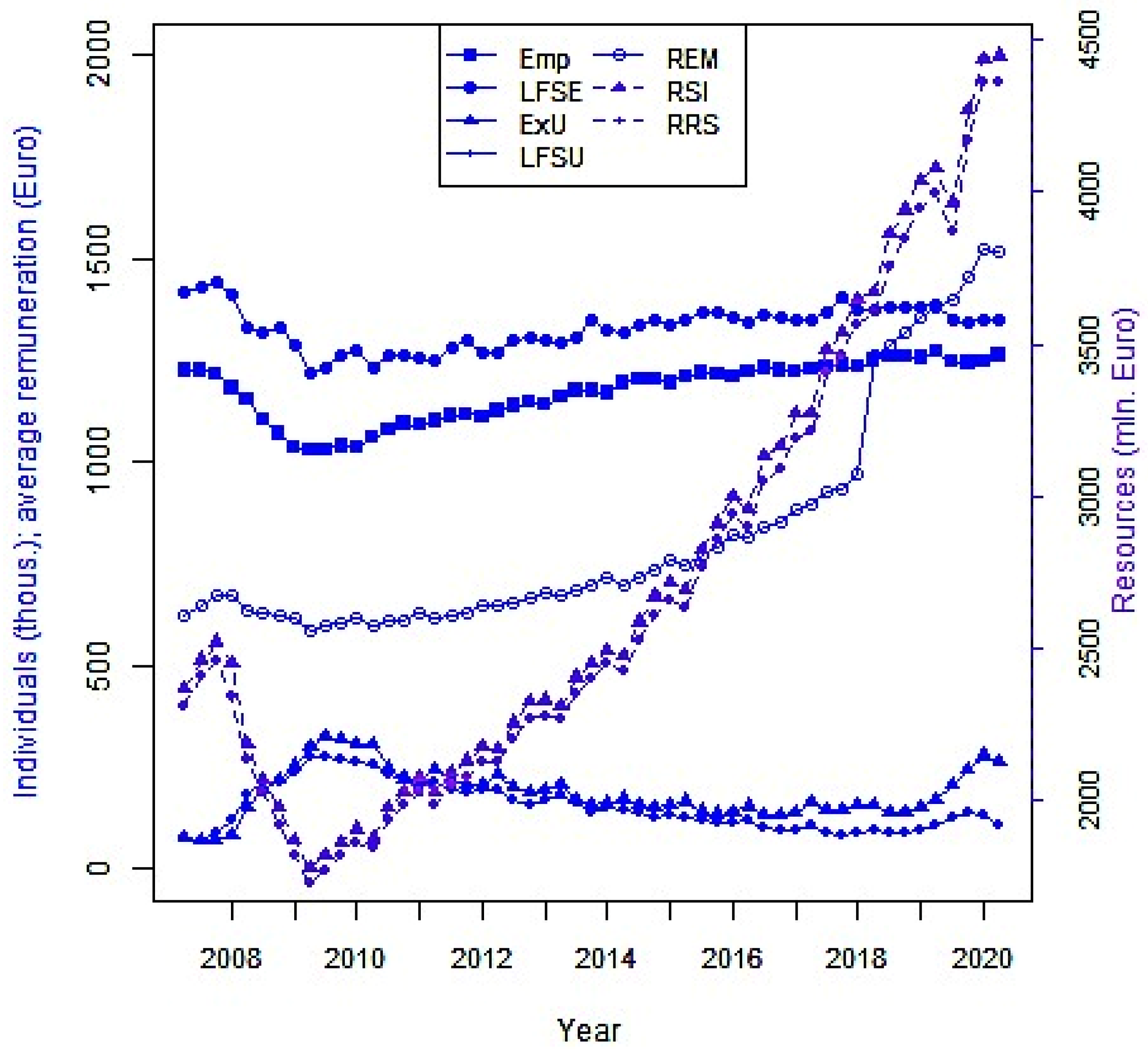
A dataset of quarterly aggregated statistics from different statistical surveys conducted by Statistics Lithuania in 2008–2021 and certain administrative data sources [37] are used for this case study. The dataset is presented in Table A1. It consists of 53 quarterly observations, ending with the 1st quarter of 2021. The seven indicators studied are as follows:

• Labour Force Survey variables: number of employed persons (LFSE); number of the unemployed (LFSU), in thousand;
• Labour Remuneration Survey data: number of employees (Emp), in thousand; enterprise resources for remuneration (RRS), in EUR million;
• Labour Exchange Office data: number of the registered unemployed (ExU), in thousand;
• Administrative data of the State Social Insurance Fund Board: enterprise remuneration from which taxes are paid (RSI), in EUR million; Average wages and salaries of employees, excluding individual enterprises (average remuneration), in EUR (REM).

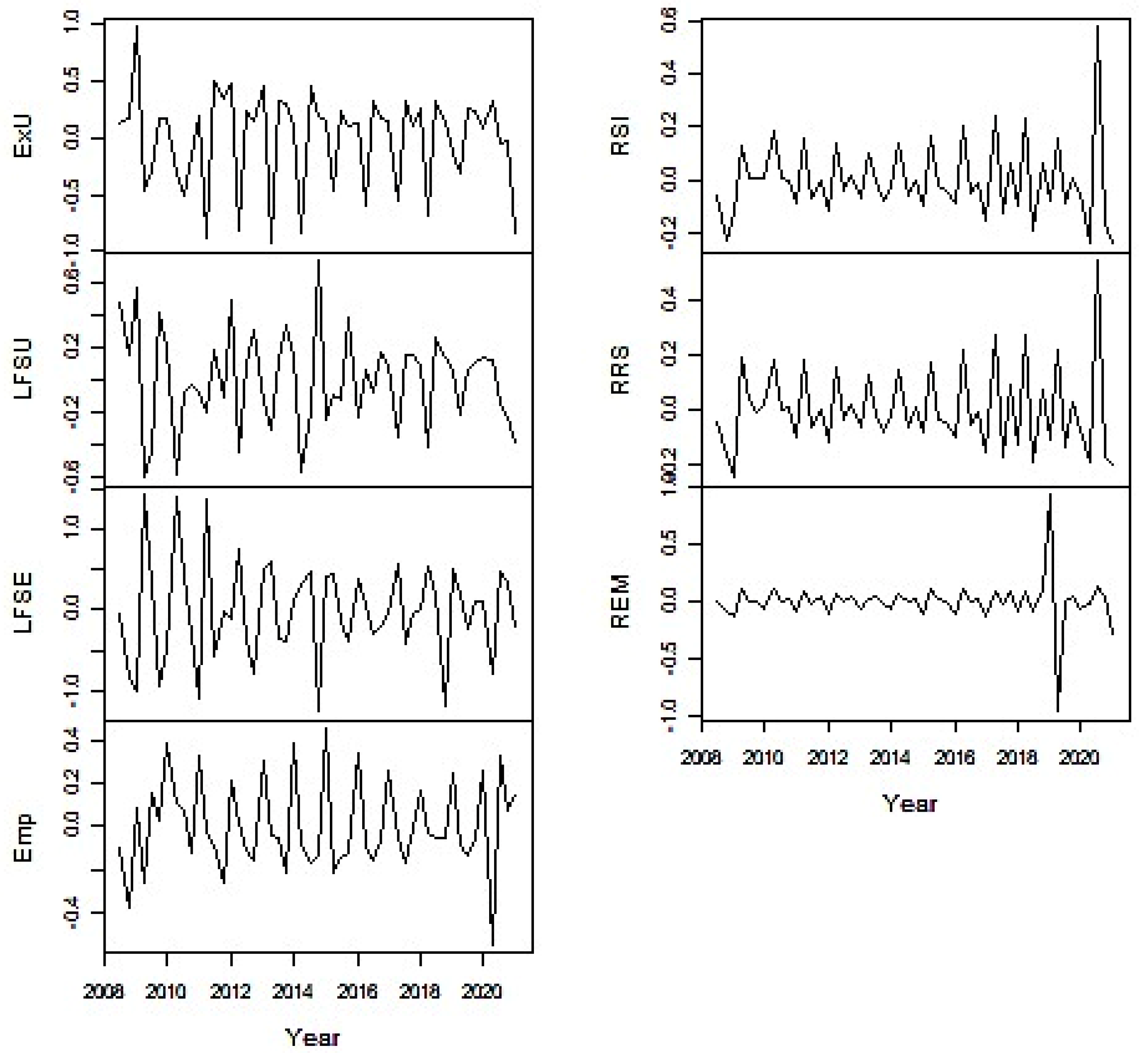
These time series are represented in Figure 2 using two vertical axes. The left-side vertical axis is for the indicators meaning the number of individuals (Emp, LFSU, ExU, LFSE) and average wages and salaries (REM). The right-side vertical axis is for the indicators expressed in EUR million (RSI, RRS).

The indicators have been chosen in order to ensure their diversity for further analysis. Figure 2 shows similar trends in the pairs of time series: the number of employed persons (LFSE) from the Labour Force Survey and the number of employees (Emp) from the Labour Remuneration Survey; the number of the unemployed (LFSU) from the Labour Force Survey and the number of the registered unemployed (ExU) from the Labour Exchange Office. These two pairs of indicators match each other well: as the number of employed persons increases, the number of the unemployed decreases, and vice versa. It would seem that they satisfy the definition of coherence provided in the OECD Glossary [6]. However, the coherence of the time series is not about their trends. Rather, it is about the linear dependency between the components of the Fourier transforms of the stationary time series corresponding to the same frequency.

4.2. Data Analysis for Ordinary Coherence

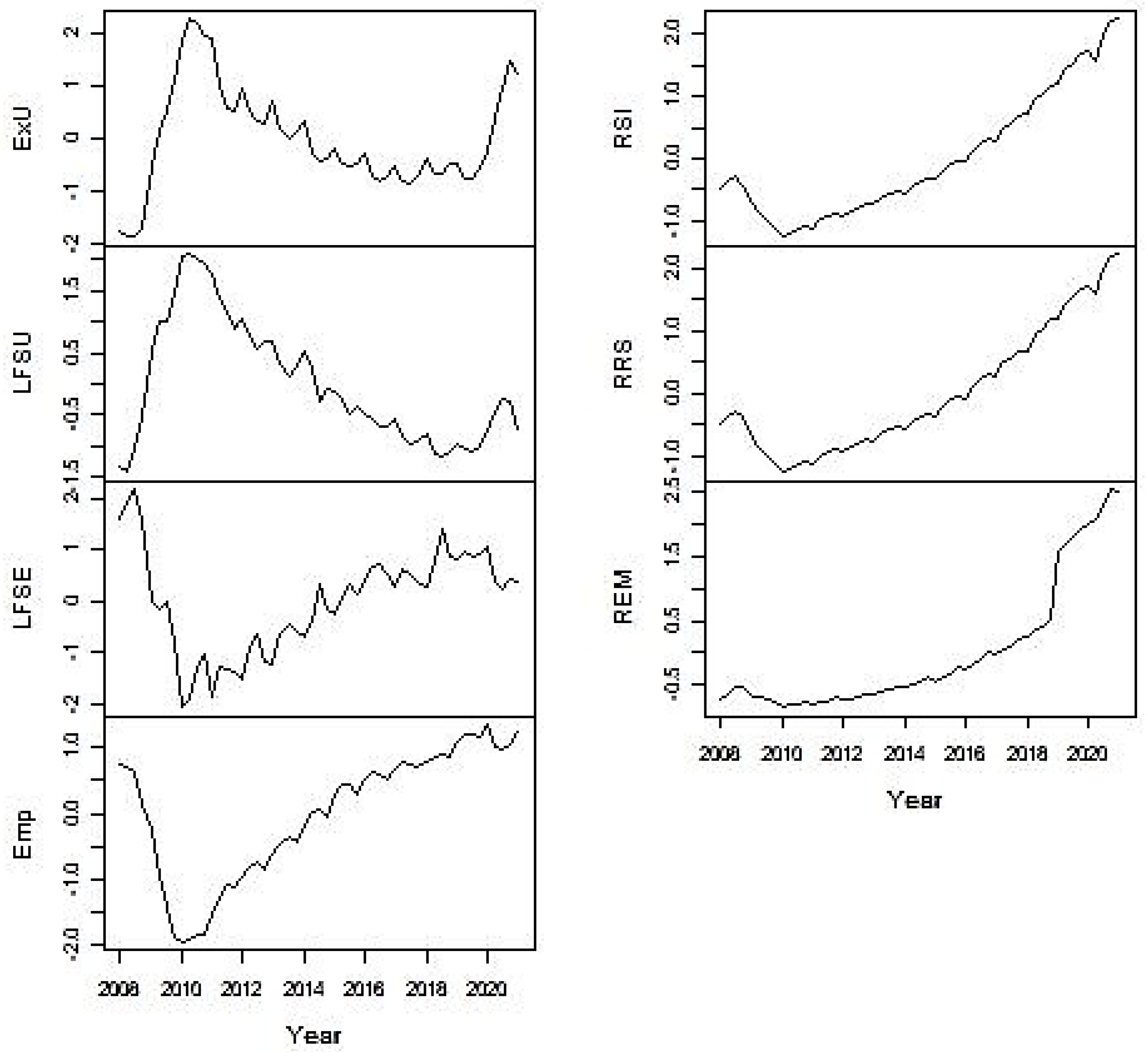
The data series used for this study are not stationary according to the augmented Dickey–Fuller test for the unit root [38]. In order to reach their stationarity, the third-order polynomial trend is excluded from the two time series of the unemployed, and the second-order polynomial trend is excluded from the remaining five time series using the least squares method. The standardised residuals are presented in Figure 3. Unfortunately, only three detrended time series have been recognized as stationary by the augmented Dickey–Fuller test: Emp (p = 0.08), RSI (p = 0.03), and RRS (p = 0.03). Some long-period waves can be observed in certain graphs of detrended and standardized time series in Figure 3, and they may determine the declination of the detrended time series from stationarity.

Signal processing researchers also face the problem of non-stationarity. One of the ways to wriggle out of this difficulty is to divide the signals into short time blocks, so as to capture the time dependency and, by restricting the signal to each of the individual blocks, enable it to be considered stationary (i.e., a pseudo-stationary approach). Then, one of the methods valid for stationary signals is applied to each block (Gonzales [39]). Our detrended time series are short: too short to be divided into the blocks. So, let us further assume that all of them are stationary.

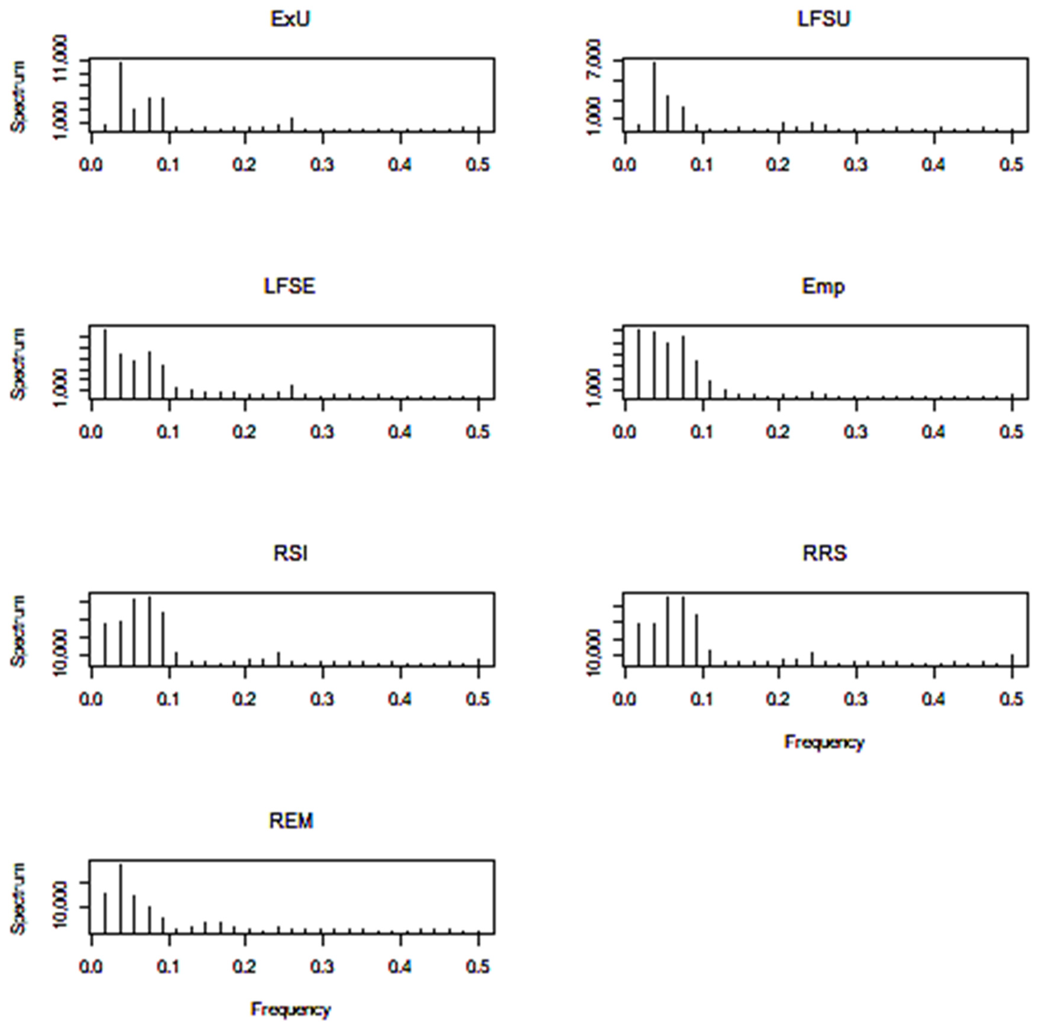
Periodograms—squared coefficients of the periodic components in the time series Fourier representation against frequencies—for all of the time series are calculated, and their graphs are presented in Figure 4. The R program function spec.pgram (R stats package [40]) with the nonparametric smoothing of the sample periodogram is used [16]. A modified Daniell kernel is used for this purpose.

All of the periodograms show high spectrum values corresponding to low frequencies. They inform us about the importance of the corresponding periodic components in the Fourier representation. Since we have quarterly data, we can expect to find in our time series periods equal to several years or 4k quarters, k = 1,2, …. One-, two-, four- or eight-year cycles correspond to the frequencies $\omega =1/4k$: 0.25, 0.125, 0.0625, 0.03275. Therefore, we see periodogram peaks for low frequencies and the eight-year cycle in some graphs of Figure 4. We also see a small peak in the periodogram at the obvious yearly cycle for the frequency ω = 0.25. It is a natural cycle in our quarterly data, and most of our further attention will be directed towards it.

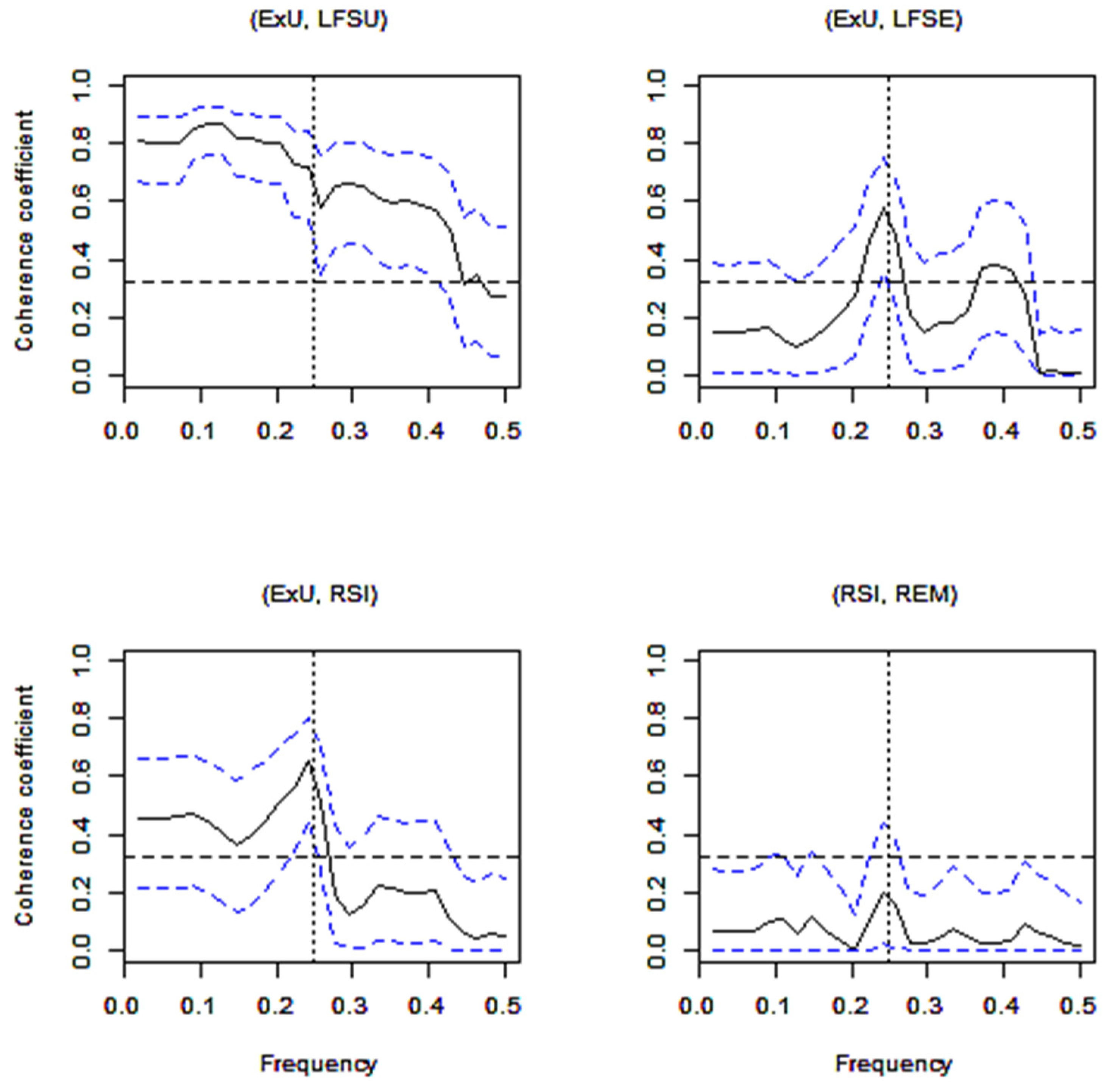
Some visualisations of the coherence coefficients are presented in Figure 5. Squared coherence is presented for frequencies $0\le \omega \le 0.5$. It is drawn in a black solid line. The 0.95-level confidence interval for the coherence coefficient is drawn in dashed blue lines. The hypothesis about the equality of the coherence coefficient to 0 is tested by the approximate F test [16] and is rejected for the coherence coefficient greater than $c=0.226$ with the significance level α = 0.01. The dashed black horizontal line on the graph means that the values of the coherence coefficient lower than c for any frequency are insignificant. Our interest lies mostly with the frequency $\omega =0.25$, and a vertical line is drawn at this frequency in order to address the reader to the value of the squared coherence at this frequency.

Figure 5 shows quite high coefficients of coherence for the frequencies ω ≤ 0.25 between the two indicators of unemployment ExU and LFSU, and between the indicators of the registered unemployed (ExU) and enterprise remuneration from which taxes are paid (RSI). The number of the registered unemployed (ExU) from the Labour Exchange Office and the number of employed persons (LFSE) from the Labour Force Survey have a significant coefficient of coherence only for ω = 0.25. Meanwhile, the indicators of enterprise remuneration from which taxes are paid (RSI) from the State Social Insurance Fund Board and average wages and salaries of employees (REM) do not have a significant coherence coefficient for all frequencies.

All of the coherence coefficients of the indicators studied at frequency $\omega =0.25$ are presented in

Table 1. Coherence matrix at frequency $\omega =0.25$.

	ExU	LFSU	LFSE	Emp	RSI	RRS	REM
ExU	1.000
LFSU	0.581	1.000
LFSE	0.482	0.347	1.000
Emp	0.466	(0.159)	0.590	1.000
RSI	0.513	0.312	0.573	0.497	1.000
RRS	0.517	0.317	0.590	0.505	0.985	1.000
REM	(0.186)	(0.054)	(0.034)	(0.045)	(0.154)	(0.145)	1.000

. Insignificant coefficients with the significance level α = 0.01 are taken into brackets. The indicator of average wages and salaries of employees (REM) does not have any significant coefficient of coherence with all of the indicators studied. A very high coefficient of coherence (0.985) is observed between RRS (enterprise resource for remuneration) and RSI (enterprise remuneration from which taxes are paid), that is, between survey data and administrative source data.

4.3. Data Analysis for Granger Causality

In order to satisfy an assumption on weakly stationary time series for the causality study, the initial variables were standardised and the second-order differences from the standardised variables were extracted. According to the augmented Dickey Fuller test with the significance level α = 0.05 all of the resulting variables become weakly stationary (Figure 6).

The lag size m included in (4), (5) is estimated applying Schwarz information criteria [41]. For almost all variables this statistic reaches its minimum value at $m=4$. Therefore, the Granger causality is tested with this lag value m = 4. The hypothesis H0: x_t is not the Granger cause for y_t against the alternative $H1:x_t\Rightarrow y_t$ is tested by an approximate F test using F(m,n-(2m + 1)) statistics. The results are presented in

Table 2. Coherence and causality at frequency ω = 0.25.

	ExU	LFSU	LFSE	Emp	RSI	RRS	REM
ExU	1			F = 4.0304 p = 0.0080 ⟸	F = 2.2583 p = 0.0808 ⟸
LFSU	0.5777	1	F = 2.9724 p = 0.0313 ⟸	F = 3.598 p = 0.0139 ⟸
LFSE	0.5458	0.5509	1
Emp	0.3540	(0.2115)	0.2765	1	F = 2.4902 p = 0.0593 ⟹	F = 2.7536 p = 0.0418 ⟹
RSI	(0.1235)	(0.1462)	0.2609	(0.0765)	1	F = 2.9798 p = 0.0310 ⟹ F2.1892 p = 0.0886 ⟸	F = 2.4902 p = 0.0593 ⟸
RRS	(0.2144)	(0.2125)	0.3209	(0.0720)	0.9554	1	F = 2.7536 p = 0.0418 ⟸
REM	(0.0190)	(0.0049)	(0.0533)	(0.0082)	(0.0209)	(0.0125)	1

. Its lower left triangle includes coherence coefficients. The upper right triangle includes the results of the Granger causality test. It includes in each cell the value of the empirical test statistics F, p-value and arrow. This arrow from left to right means that the indicator on the line is a cause for the indicator in the column. The arrow from the right to the left means that the column indicator is a cause for the line indicator.

Ordinary coherence coefficients for ω = 0.25 are presented in Table 2. Logical Granger causality cases are observed: the number of employed persons estimated based on the Labour Force Survey data is a Granger cause for the number of the unemployed estimated in the same survey; average wages and salaries is a cause for the resources for remuneration. It is seen that there is feedback relation between two indicators: RSI and RR, and their coherence coefficient is high for both methods. Let us compare the following results:

• LFSE ⟹ LFSU, $co{h}^2(\mathrm{LFSU},\mathrm{LFSE}|\omega =0.25)=0.577$;
• Emp ⟹ ExU, $co{h}^2(\mathrm{Emp},\mathrm{ExU}|\omega =0.25)=0.354$.

In these cases the hypothesis about no Granger causality is rejected, and coherence coefficients between the variables are also significant. Other cases:

3.

Emp ⟹ RSI, $co{h}^2(\mathrm{Emp},\mathrm{RSI}|\omega =0.25)=0.0765$;

4.

Emp ⟹ RSE, $co{h}^2(\mathrm{Emp},\mathrm{RSE}|\omega =0.25)=0.0720$.

In the last cases, coherence coefficients are not significant despite the fact that the hypothesis about no Granger causality is rejected. Now let us compare coherence coefficients with the corresponding ones in Table 1:

5.

$co{h}^2(\mathrm{LFSU},\mathrm{LFSE}|\omega =0.25)=0.347; co{h}^2(\mathrm{Emp},\mathrm{ExU}|\omega =0.25)=0.466$;

6.

$co{h}^2(\mathrm{Emp},\mathrm{RSI}|\omega =0.25)=0.497; co{h}^2(\mathrm{Emp},\mathrm{RSE}|\omega =0.25)=0.5$.

The estimated coefficients in Case 5 can be compared with the corresponding coefficients in cases 1 and 2. However, Case 6 differs from cases 3 and 4.

Two methodological approaches have been proposed to estimate ordinary coherence coefficient. The results of the coherence coefficient estimation have similarities, but there are also differences. Lack of the stationarity in the first case may be one of the reasons. Despite the fact that the time series in both cases have the same origin, they are different, which may be another reason for certain differences in the values of coherence coefficients. We see that an unambiguous conclusion about coherence coefficient estimation in both cases cannot be drawn. The validity of the Granger causality does not necessarily mean that the coherence coefficient is significant.

4.4. Visualization of the Time Series

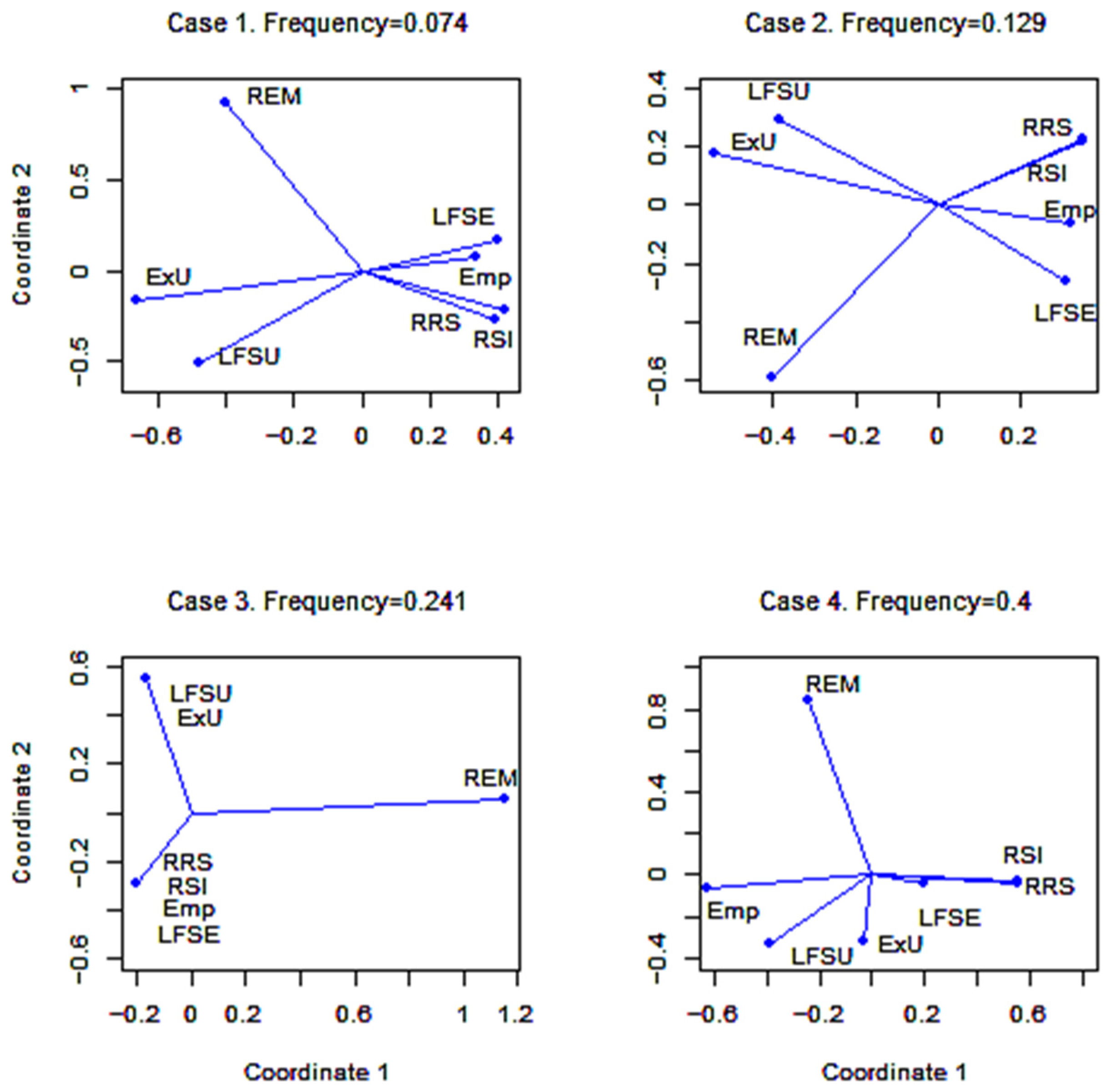
We will visualise seven time series described in Section 3.5 by applying multidimensional scaling. The four frequencies chosen are presented in

Table 3. Frequency choice for visualisation of the time series.

Case	Frequency ω	Period $\mathit{T}=1/\mathit{\omega }$ $(\mathbf{Quarters} \mathbf{of} \mathbf{the} \mathbf{Year})$	Meaning
1	0.074	13.5	3 years
2	0.129	7.75	2 years
3	0.241	4.15	1 year
4	0.4	2.5	7.5 months

.

Multidimensional scaling is implemented for the time series under study to visualize them on a plane (the dimension of the coordinate space X is $m=2$) and the four frequencies chosen. The value of the normalised stress function reached in the iterative procedure equals 0.009, which means satisfactory accuracy of the coordinates obtained. The projections of the time series to the two-dimensional space for selected frequencies are shown in Figure 7.

Each of the univariate time series is represented by a blue dot in a two-dimensional space. Rays connect these points with the origin point (0, 0). The proximity of the dot positions means the level of synchronicity of the time series at that frequency. Case 1 shows high synchronicity in two time series of the number of employed persons; two time series on resources for remuneration are also close. Two time series on the number of the unemployed are less synchronised than the previous pairs. Definitions of unemployed person in LFSU and ExU differ, and this difference is reflected in most of the cases of the Figure 7. Case 2 shows less synchronicity in the time series for employment, but perfect synchronicity in the resources for remuneration. Case 3, which corresponds to one-year period, demonstrates complete synchronicity between employment and remuneration, as well as between the time series on unemployment. The time series on average wages and salaries is separated from others in all cases. Case 4 corresponds to the period of 7.5 months, which is impossible in these time series, and the corresponding picture shows a mixture: no synchronicity between the time series on employed persons.

4.5. Software

All of the calculations are carried out with the R v. 4.1.2 software [39].

The coefficients of the second and third order polynomial trends in time series are estimated by the least squares method using the function polyfit, and the trend itself is calculated by the function polyval, both from the package pracma.

The evaluation of the presence of the unit roots in the time series and checking for their stationarity is tested by the augmented Dickey Fuller test using the function adf.test in the package tseries.

The function spec.pgram from the package stats is used to calculate the periodograms of the weakly stationary time series by the fast Fourier transform. The same function is used to smoothen the coherence with a modified Daniel smoother (using nine terms for the moving average method half interval and giving half of the weight to the smoothing interval end values), and to test the hypothesis about the significance of coherence using Fisher statistics.

The number of lags for the causality model is tested by the Schwarz’s SC statistic implemented in the function VARselect of the package vars. The Wald test for the frequency domain-based Granger causality of the time series is realized in the function grangertest of the package lmtest.

The function isoMDS of the R package MASS is used to implement multidimensional scaling.

5. Discussion

The problem of coherence has arisen to the author due to its unmeasurable usage in official statistics. The coherence of statistical output in official statistics is a very wide concept. Any of its aspects may have different measures to assess coherence strength: cross-domain, sub-annual, and annual statistics; in national accounts, internal, geographical, and over time. In the present article, a measure for coherence strength of social and economic indicators in time—a coherence coefficient known and used in other fields of science–is recalled.

The coherence coefficient is a correlation coefficient between the Fourier transforms of two statistical indicators indexed by the same frequency. It gives an undiluted measure of linear dependency of a swing in two weakly-stationary time series due to the specified frequency. This coefficient shows the level of synchrony between the Fourier transforms of the time series of the same frequency. The article reminds the definition of the ordinary coherence coefficient. The coherence matrix may show numerically meaningful relationships between the economic time series in specific frequencies, such as frequencies, corresponding to a one-year period. Besides, some examples of methods are given. One of them is a widely explored feature of the coherence to measure the strength of the causal effect between jointly weekly stationary time series, Granger causality [26,27,28,29], and it is demonstrated in the simulation study. This property can be applied in the construction of econometric models.

Coherence matrix is often used as a starting point for multivariate analysis of time series in a similar way as correlation matrix is used for multivariate analysis of random variables. Several publications illustrating this are noticed further. Principal component analysis is applied to the coherence matrix [30,31] for dimensionality reduction. Principal components analysis is applied to the cross-spectral density matrix, and coherence coefficients are calculated for the obtained principal components in [42]. A new electroencephalography coherence approach named magnitude squared coherence based on weighted canonical correlation analysis is proposed in [32]. It improves the accuracy in coherence estimation. A coherent change detection scheme using canonical correlation analysis to determine the linear dependence between the canonical coordinates of the input channels is explored in [43]. Coherence matrix-based metric is defined in [44] and used for hierarchical clustering of the random processes and to multivariate analysis of high frequency stock market values [45] since it is able to detect any possible linear relation between two times series, even at different time instants.

One of the aims of this article is to extend a range of multivariate analysis methods used together with the coherence matrix. Multidimensional scaling is a multivariate data visualisation method in a low dimensional space. This method for large genomic data set is applied in [46]. A standard Euclidean distance is used to measure the dissimilarity of the gene groups, and the main difficulty in the solution of this problem is high dimensionality of the data set. The authors in [47] study a musical opus from the point of view of three mathematical tools; multidimensional scaling is one of them. The method is applied based on two alternative metrics: the average mutual information and the fractal dimension. The results reveal significant differences in the musical styles, demonstrating the feasibility of the proposed strategy.

We propose a multidimensional scaling method of multivariate time series in frequency domain. The coherence coefficient matrix is used as a similarity matrix between the time series in the frequency domain for non-metric multidimensional scaling. This method allows following the visual changes in the time series due to the frequency change. The method may be applied to the time series classification. It can be further developed in order to improve the accuracy of the visual representation of the time series, especially for the high dimensional case. Time series visualization is studied also in [48]. Frobenius norm, generalized correlation coefficient between two matrices, principal component analysis similarity factor is used to construct the similarity measure between the time series themselves. The Fourier transform to the time series is not applied. Our proposal is new.

A matrix of ordinary coherence coefficients may serve as a basic matrix of association among the time series in frequency for other methods of multivariate analysis.

The ordinary coherence coefficient with possible applications is proposed for the usage in official statistics for quality assessment and deeper analysis of the statistical results.

References

- Li, F.F.; Cox, T.J. Digital Signal Processing in Audio and Acoustical Engineering; CRC Press: Boca Raton, FL, USA, 2019. [Google Scholar]
- Cohen, D.; Tsuchiya, N. The Effect of Common Signals on Power, Coherence and Granger Causality: Theoretical Review, Simulations, and Empirical Analysis of Fruit Fly LFPs Data. Front. Syst. Neurosci. 2018, 12, 30. [Google Scholar] [CrossRef] [PubMed]
- Sun, F.T.; Miller, L.M.; D’Esposito, M. Measuring interregional functional connectivity using coherence and partial coherence analyses of fMRI data. NeuroImage 2004, 21, 647–658. [Google Scholar] [CrossRef] [PubMed]
- Kock, W.E. Wave Coherence. In Engineering Applications of Lasers and Holography; Springer: Boston, MA, USA, 1975. [Google Scholar]
- Eurostat. European Statistics Code of Practice, 2nd ed.; Eurostat: Luxembourg, 2017; Available online: https://ec.europa.eu/eurostat/web/products-catalogues/-/KS-02-18-142 (accessed on 8 January 2022).
- OECD. Glossary of Statistical Terms. Available online: https://stats.oecd.org/glossary/ (accessed on 8 January 2022).
- Statistics Canada. Statistics Canada Quality Guidelines, 6th ed.; Statistics Canada: Ottawa, ON, Canada, 2019; pp. 14–15. Available online: https://www150.statcan.gc.ca/n1/pub/12-539-x/12-539-x2019001-eng.htm (accessed on 8 January 2022).
- Australian Bureau of Statistics. Available online: https://www.abs.gov.au/ (accessed on 8 January 2022).
- Eurostat. ESS Handbook for Quality Reports; Eurostat: Luxembourg, 2014; Available online: http://ec.europa.eu/eurostat/web/ess/-/the-ess-handbook-for-quality-reports-2014-edition (accessed on 8 January 2022).
- European Commission. ESSnet on Quality of Multisource Statistics—Komuso; Eurostat: Luxembourg, 2019; Available online: https://ec.europa.eu/eurostat/cros/content/essnet-quality-multisource-statistics-komuso_en/ (accessed on 8 January 2022).
- Pankūnas, V.; Janeiko, J.; Krapavickaitė, D. Coherence studies in time series. In Proceedings of the Workshop of Baltic-Nordic-Ukrainian Network on Survey Statistics, Jelgava, Latvia, 21–25 August 2018; pp. 66–69. Available online: http://www.statistikuasociacija.lv/workshop2018/files/papers/BNU2018-Pank%C5%ABnas-and-Janeiko.pdf (accessed on 3 March 2022).
- Till-Tentschert, U. Coherence Assessment of EU-SILC in Austria, 2006. In Proceedings of the Conference and Methodological Workshop “Comparative EU Statistics on Income and Living Conditions: Issues and Challenges”, Finland, Helsinki, 6–8 November 2006; Available online: https://www.stat.fi/eusilc/ws_5-2_till.pdf (accessed on 8 January 2022).
- African Development Bank. Labour Force Data Analysis: Guidelines with African Specificities; African Development Bank: Tunis, Tunisia, 2012; pp. 92–97. Available online: https://www.afdb.org/fileadmin/uploads/afdb/Documents/Publications/Labour%20Force%20Data%20Analysis_WEB.pdf (accessed on 8 January 2022).
- Eurostat. Quality Report of the European Union Labour Force Survey 2015; Eurostat: Luxembourg, 2017; pp. 28–32. Available online: http://ec.europa.eu/eurostat/documents/7870049/7887033/KS-FT-17-003-EN-N.pdf/22ed8f4e-9eb3-455c-924a-8df102620f89 (accessed on 8 January 2022).
- Wiener, N. Generalized harmonic analysis. Acta Math. 1930, 55, 117–258. [Google Scholar] [CrossRef]
- Shumway, R.H.; Stoffer, D.S. Time Series Analysis and Its Applications: With R Examples; Springer: Berlin/Heidelberg, Germany, 2006. [Google Scholar]
- Wei, W.W.S. Time Series Analysis: Univariate and Multivariate Methods; Pearson Education: London, UK, 2006. [Google Scholar]
- Bendat, J.S.; Piersol, A.G. Random Data. Analysis and Measurement Procedures; Wiley-Interscience: Hoboken, NJ, USA, 2010. [Google Scholar]
- Papana, A. Connectivity Analysis for Multivariate Time Series: Correlation vs. Causality. Entropy 2021, 23, 1570. [Google Scholar] [CrossRef] [PubMed]
- Yue, J.; Takaahara, G.; Franczak, B.; Burr, W.S. Time Series Clustering using Coherence. In Proceedings of the 2nd International Conference on Statistics: Theory and Applications (ICSTA’20), Prague, Czech Republic, 19–21 August 2020. [Google Scholar] [CrossRef]
- Euán, C.; Sun, Y.; Ombao, H. Coherence-based time series clustering for statistical inference and visualization of brain connectivity. Ann. Appl. Stat. 2019, 13, 990–1015. [Google Scholar] [CrossRef] [Green Version]
- Foster, M.R.; Guinzy, N.J. The Coefficient of Coherence: Its estimation and Use in Geophysical Data Processing. Geophysics 1967, 32, 602–616. [Google Scholar] [CrossRef]
- Koopmans, L.H. On the Coefficient of Coherence for Weakly Stationary Stochastic Processes. Ann. Math. Stat. 1964, 35, 532–549. [Google Scholar] [CrossRef]
- Granger, C.W. Investigating causal relations by econometric models and cross-spectral methods. Econometrica 1969, 37, 424–438. [Google Scholar] [CrossRef]
- Breitung, J.; Candelon, B. Testing for short- and long-run causality: A frequency-domain approach. J. Econom. 2006, 132, 363–378. [Google Scholar] [CrossRef]
- Contreras-Reyes, J.E.; Hernández-Santoro, C. Assessing Granger-causality in the southern Humboldt current ecosystem using cross-spectral methods. Entropy 2021, 22, 1071. [Google Scholar] [CrossRef]
- Borlaf-Mena, I.; Badea, O.; Tanase, M.A. Assessing the Utility of Sentinel-1 Coherence Time Series for Temperate and Tropical Forest Mapping. Remote Sens. 2021, 13, 4814. [Google Scholar] [CrossRef]
- Kayer, A.S.; Sun, T.C.; D’Esposito, M. A Comparison of Granger causality and Coherency in fMRI-Based Analysis of the Motor System. Hum. Brain Mapp. 2009, 30, 3475–3494. [Google Scholar]
- Faes, L.; Erla, S.; Porta, A.; Nollo, G. A framework for assessing frequency domain causality in physiological time series with instantaneous effects. Philos. Trans. R. Soc. A 2013, 371, 20110618. [Google Scholar] [CrossRef] [PubMed] [Green Version]
- Liu, Z.; Song, C.; Cai, H.; Yao, X.; Hu, G. Enhanced coherence using principal component analysis. Interpretation 2017, 5, T351–T359. [Google Scholar] [CrossRef]
- Le, N.; Song, S.; Zhang, Q.; Wang, R. Robust principal component analysis in optical micro-angiography. Quant. Imaging Med. Surg. 2017, 7, 654–667. Available online: https://qims.amegroups.com/article/view/17862 (accessed on 8 January 2022). [CrossRef] [PubMed] [Green Version]
- Cui, D.; Qi, S.; Gu, G.; Li, X.; Li, Z.; Wang, L.; Yin, S. Magnitude Squared Coherence Method based on Weighted Canonical Correlation Analysis for EEG Synchronization Analysis in Amnesic Mild Cognitive Impairment of Diabetes Mellitus. IEEE Trans. Neural Syst. Rehabil. Eng. 2018, 26, 1908–1917. [Google Scholar] [CrossRef]
- Zhao, Y.; Wachowski, N.; Azimi-Sadjadi, M.R. Target Coherence Analysis Using Canonical Correlation Decomposition for SAS Data. In Proceedings of the OCEANS 2009, Biloxi, MS, USA, 26–29 October 2009. [Google Scholar] [CrossRef]
- Nedungadi, A.G.; Ding, M.; Rangarajan, G. Block coherence: A method for measuring the interdependence between two blocks of neurobiological time series. Biol. Cybern. 2011, 104, 197–207. [Google Scholar] [CrossRef]
- Borg, I.; Groenen, P.J.F. Modern Multidimensional Scaling; Springer: Berlin/Heidelberg, Germany, 2005. [Google Scholar]
- Dzemyda, G.; Kurasova, O.; Žilinskas, J. Multidimensional Data Visualization, Methods and Applications; Springer: Berlin/Heidelberg, Germany, 2013. [Google Scholar]
- Statistics Lithuania: Official Statistics Portal. Available online: https://osp.stat.gov.lt/ (accessed on 20 January 2022).
- Dickey, D.A.; Fuller, W.A. Distribution of the estimates for autoregressive time series with a unit root. J. Am. Stat. Assoc. 1979, 74, 427–431. [Google Scholar]
- Gomez Gonzalez, A.; Rodrıguez, J.; Sagartzazu, X.; Schuhmacher, A.; Isasa, I. Multiple coherence method in time domain for the analysis of the transmission paths of noise and vibrations with non-stationary signals. In Proceedings of the ISMA2010 International Conference on Noise and Vibration Engineering including USD2010; Sas, P., Bergen, B., Eds.; Katholieke Universiteit Leuven: Leuven, Belgium, 2010; pp. 3927–3942. [Google Scholar]
- The Comprehensive R Archive Network. Available online: https://cran.r-project.org/ (accessed on 8 January 2022).
- Schwarz, G. Estimating the dimension of a model. Ann. Stat. 1978, 6, 461–464. [Google Scholar] [CrossRef]
- Huang, Y.; Fergusson, N. Principal component analysis of the cross-axis apparent mass nonlinearity during whole-body vibration. Mech. Syst. Signal Process. 2021, 146, 107008. [Google Scholar] [CrossRef]
- Tesfaye, G.-M.; Tucker, J.D. Canonical correlation analysis for coherent change detection in synthetic aperture Sonar Imagery. Inst. Acoust. Proc. 2010, 32, 117–122. [Google Scholar]
- Innocenti, G.; Materassi, D. Econometrics as Sorcery. Statistical Finance (q-fin.ST). arXiv 2008, arXiv:0801.3047. [Google Scholar] [CrossRef]
- Materassi, D.; Innocenti, G. Coherence-based multivariate analysis of high frequency stock market values. arXiv 2008, arXiv:0805.2713. [Google Scholar] [CrossRef]
- Tzeng, J.; Lu, H.H.S.; Li, W.H. Multidimensional scaling for large genomic data sets. BMC Bioinform. 2008, 9, 179. [Google Scholar] [CrossRef] [PubMed] [Green Version]
- Lima, M.F.M.; Machado, J.A.T.; Costa, A.C. A Multidimensional Scaling Analysis of Musical Sounds Based on Pseudo Phase Plane. Abstr. Appl. Anal. 2012, 2012, 436108. [Google Scholar] [CrossRef] [Green Version]
- Bernatavičienė, J.; Dzemyda, G.; Bazilevičius, G.; Medvedev, V.; Marcinkevičius, V.; Treigys, P. Method for visual detection of similarities in medical streaming data. Int. J. Comput. Commun. Control 2015, 10, 8–21. [Google Scholar] [CrossRef] [Green Version]
Figure 1.
Coherent and incoherent waves.
Figure 2.
Time series studied.
Figure 3.
Time series after the exclusion of polynomial trends and standardization.
Figure 4.
Periodograms.
Figure 5.
Visualisations of coherence coefficients (in black) and their 0.95-level confidence interval (in blue).