
Differential Elite Learning Particle Swarm Optimization for Global Numerical Optimization


School of Artificial Intelligence, Nanjing University of Information Science and Technology, Nanjing 210044, China
*
Author to whom correspondence should be addressed.
Mathematics 2022, 10(8), 1261; https://0-doi-org.brum.beds.ac.uk/10.3390/math10081261
Submission received: 12 March 2022
/
Revised: 4 April 2022
/
Accepted: 8 April 2022
/
Published: 11 April 2022
(This article belongs to the Special Issue Recent Advances in Computational Intelligence and Its Applications)
Abstract
:Although particle swarm optimization (PSO) has been successfully applied to solve optimization problems, its optimization performance still encounters challenges when dealing with complicated optimization problems, especially those with many interacting variables and many wide and flat local basins. To alleviate this issue, this paper proposes a differential elite learning particle swarm optimization (DELPSO) by differentiating the two guiding exemplars as much as possible to direct the update of each particle. Specifically, in this optimizer, particles in the current swarm are divided into two groups, namely the elite group and non-elite group, based on their fitness. Then, particles in the non-elite group are updated by learning from those in the elite group, while particles in the elite group are not updated and directly enter the next generation. To comprise fast convergence and high diversity at the particle level, we let each particle in the non-elite group learn from two differential elites in the elite group. In this way, the learning effectiveness and the learning diversity of particles is expectedly improved to a large extent. To alleviate the sensitivity of the proposed DELPSO to the newly introduced parameters, dynamic adjustment strategies for parameters were further designed. With the above two main components, the proposed DELPSO is expected to compromise the search intensification and diversification well to explore and exploit the solution space properly to obtain promising performance. Extensive experiments conducted on the widely used CEC 2017 benchmark set with three different dimension sizes demonstrated that the proposed DELPSO achieves highly competitive or even much better performance than state-of-the-art PSO variants.
Keywords:
particle swarm optimization; differential elite learning; swarm intelligence; global optimization; multimodal problemsMSC:
68-04; 65-041. Introduction
Particle swarm optimization (PSO) has received extensive attention since it was proposed by Eberhart and Kennedy in 1995 [1]. By means of its easiness in implementation, strong global search ability, and no requirement for the mathematical properties of optimization problems, it has been widely used to solve various optimization problems [2] and has been widely used to solve real-world engineering problems, such as influence spread [3] and Hilbert transform [4].
In PSO, the most critical part is the learning strategy to update particles. In the classical PSO, each particle learns from its own historical best position and the global best position of the swarm discovered so far [1,5]. Such a learning strategy has two limitations [6,7]. On the one hand, the global best position is too greedy. On the other hand, the global best position is shared by all particles. These two limitations lead to a low learning diversity of particles. Therefore, the classical PSO loses its effectiveness when solving multimodal problems [8]. To improve the optimization performance of PSO, many researchers have been devoted to designing novel learning strategies to improve the learning effectiveness and the learning diversity of particles. As a result, many remarkable advanced learning strategies [9,10,11,12,13,14] have been developed. Roughly speaking, existing learning strategies of PSO can be divided into two main categories, namely topology-based learning strategies [15,16,17] and exemplar construction based learning strategies [18,19,20].
Topology-based learning strategies [5,15,21,22,23] mainly utilize different topologies to communicate with other particles and find suitable guiding exemplars for each particle. To avoid falling into local regions and premature convergence, neighborhood topology structures are commonly employed to increase the learning diversity of particles to explore the solution space. In this research direction, many topologies have been developed, such as the ring topology [24], the star topology [25], the wheel topology [5], the random topology [26,27], and the dynamic topology [28].
Different from topology-based learning strategies, exemplar construction-based strategies [10,29,30,31] mainly construct a new guiding exemplar for each particle by using various dimension recombination techniques. In general, the constructed exemplar is not visited by particles in the swarm. In this research direction, the most representative method is the comprehensive learning PSO (CLPSO) [10], which constructs a guiding exemplar dimension by dimension based on the personal best positions of all particles. Since the advent of CLPSO, many other effective recombination techniques have been devised, such as the orthogonal learning PSO (OLPSO) [29], which designs an orthogonal matrix to roughly seek for the effective recombination of dimensions, and the genetic learning PSO (GLPSO) [31], which uses operators in genetic algorithms to construct a guiding exemplar for each particle.
The above two main kinds of learning strategies mainly utilize the historical best positions, such as the personal best positions, the global best position, and the neighbor best positions, to direct the update of particles. These historical best positions usually remain unchanged for many generations, especially in the late stage of the evolution, leading to the learning effectiveness and the learning diversity of particles being improved limitedly. To alleviate this issue, in recent years, many researchers have attempted to abandon the use of this historical information to direct the update of particles, but turn to utilizing the predominant particles in the current swarm to direct the update of inferior ones. Along this line, many novel PSO variants have been developed [9,32,33,34], such as the competitive swarm optimizer (CSO) [33], and the level-based learning swarm optimizer (LLSO) [35]. When compared with traditional PSO variants utilizing historical information to direct the update of particles, these new PSO variants preserve higher search diversity because particles in the current swarm are updated generation-by-generation, and thus the predominant particles in the current swarm used to direct the update of inferior ones are different in different generations.
Taking inspiration from the idea of employing predominant particles in the current swarm to guide the update of particles, this paper proposes a differential elite learning particle swarm optimization (DELPSO) algorithm to further improve the optimization performance of PSO. Specifically, instead of randomly adopting predominant particles in the swarm to guide the update of inferior one in existing studies [33,34,36,37], the proposed DELPSO adopts two very differential predominant particles to update inferior ones, so that each particle could learn from two very different exemplars, and thus the learning diversity of particles is further improved largely. In particular, the main features and main components are summarized as follows:
- (1)
- A differential elite learning strategy (DEL) is devised to update particles. Specifically, this strategy first divides the swarm into two exclusive sets, namely the elite group (EG) containing the top best egs (egs is the size of EG) particles and the non-elite group (NEG) containing the rest. Then, particles in the elite group are not updated, and only particles in the non-elite group are updated by learning from those in the elite group. To compromise a promising balance between fast convergence and high diversity, we let each particle in the non-elite group learn from two very differential exemplars. In this way, the learning diversity and the learning effectiveness of particles could be promoted largely.
- (2)
- A dynamic partition strategy for separating the swarm into the two groups is further devised by dynamically adjusting the elite group size. Specifically, the elite group size is gradually decreased from a large value to a small value. In this way, more and more particles come into the non-elite group and then are updated by learning from fewer and fewer elites in the elite group. With this mechanism, the swarm gradually changes from exploring the solution space to exploiting the promising areas.
With the above mechanisms, the proposed DELPSO is expected to balance high search diversity and fast convergence well, in order to explore and exploit the solution space to achieve satisfactory performance. To verify its effectiveness, extensive experiments were carried out on the CEC 2017 benchmark problem set [38] with three dimension sizes (namely 30, 50, and 100) by comparing DELPSO with several state-of-the-art PSO variants. In addition, deep investigations on the effectiveness of each component in DELPSO were also performed to find what contributes to its promising performance in solving optimization problems.
The rest of this paper is organized as follows. In Section 2, the closely related work is briefly reviewed. Section 3 elaborates the proposed DELPSO in details, and Section 4 carries out extensive experiments to validate the effectiveness of DELPSO. At last, the conclusion of this paper is given in Section 5.
2. Related Work
2.1. Canonical Particle Swarm Optimization
In PSO [1], each particle is represented by two vectors, namely the position vector and the velocity vector , where , is the population size and is the dimension size. In the classical PSO, each particle cognitively learns from its own experience and socially learns from the social experience of the whole swarm. In particular, each particle is updated as follows:
where is the personal best position of the th particle and is the global best position found so far by the whole swarm. In terms of the parameters, ω is the inertia weight, and are two acceleration coefficients, and are two real random numbers uniformly sampled within (0,1).
In Equation (1), it is found that in the classical PSO, all particles share one same guiding exemplar, namely the global best position of the swarm . Besides, such a guiding exemplar is too greedy. These two limitations lead to the classical PSO preserving low search diversity but having fast convergence. Hence, it usually obtains promising performance on unimodal problems, but loses its effectiveness on multimodal problems [6,39].
2.2. Development of PSO
To improve the optimization performance of PSO, researchers have been devoted to designing novel PSO variants from different perspectives. For example, to alleviate the sensitivity of PSO to the parameters in Equation (1), researchers have devised many adaptive parameter adjustment strategies [40,41,42]. To improve the learning effectiveness of particles, researchers have proposed a lot of novel and effective learning strategies for PSO [10,34,43,44].
Among the extensive research of PSO, the most widely researched direction is the learning strategies for PSO, which play a vital role in helping PSO achieve good performance. In a broad sense, existing learning strategies for PSO can be classified into two main categories, namely topology-based learning strategies [15,21,28,45,46] and constructive learning strategies [10,18,29,47,48].
Topology-based learning strategies mainly make use of different topological structures to communicate with other particles to find appropriate exemplars to guide the updating of each particle. In fact, the learning strategy in classical PSO [1,5] is a global topology based one, where all particles are connected to interchange information. Such a full topology usually leads to greedy attraction of the second guiding exemplar in Equation (1), which likely results in premature convergence of PSO in solving multimodal problems. To alleviate this issue and to reduce the greedy attraction of the second guiding exemplar, researchers have developed many neighborhood topologies to increase the diversity of the second exemplar in Equation (1), in order to improve the performance of PSO [5,22,23]. For instance, in [15], a ring topology along with a local search method was introduced into PSO to maintain the balance between exploration and exploitation. Specifically, the ring topology was used to construct a neighbor region for each particle to determine a less greedy exemplar for the associated particle, so that high swarm diversity could be maintained, and the possibility of particles being trapped in local optima could be expectedly reduced. Except for the ring topology, the star topology [5] and the wheel topology [5] were also employed to connect particles and determine a promising exemplar to replace in Equation (1) for each particle. In [49], Shi et al. adopted the cellular automata (CA) with the lattice and the “smart-cell” structure to connect particles to select the second guiding exemplar for each particles.
Since different topologies preserve different properties, to take advantage of the merits of different topologies, researchers have attempted to use multiple topologies to select guiding exemplars for particles [50,51]. For instance, Du et al. proposed a heterogeneous strategy PSO (HSPSO) [52] by using different topological structures for different particles. Specifically, some particles adopt the global topology to achieve fast convergence, while some particles adopt the local topology to maintain high diversity. In addition, instead of using fixed topologies, some researchers have even proposed to use dynamic topologies to find promising exemplars to direct the update of particles. For instance, Zeng et al. proposed a dynamic-neighborhood-based switching PSO (DNSPSO) algorithm [28] by devising a distance-based dynamic topology and a novel switching learning strategy to adaptively adjust the topology based on the state of the swarm. In [53], a small-world network based topology was designed to let each particle interact with its nearest neighbors with a high probability and to communicate with some distant particles with a low probability.
Instead of selecting exemplars from existing personal best positions of particles, constructive learning strategies [10,30,47,48,54] mainly construct promising guiding exemplars for particles by recombining dimensions of historical best positions. In this research direction, the most representative algorithm is the comprehensive learning particle swarm optimizer (CLPSO) [10]. Specifically, in this algorithm, a guiding exemplar is constructed dimension-by-dimension, based on the selected personal best positions. Due to the randomness in the selection of the personal best positions, the constructed exemplars are likely different for different particles, and thus CLPSO shows good performance in solving multimodal problems. To further improve the optimization performance of CLPSO, many effective techniques have been additionally proposed to cooperate with CLPSO to achieve more promising performance [30,54,55]. For instance, Lynn et al. proposed a heterogeneous CLPSO in [47]. Specifically, this algorithm first divides the swarm into two subgroups. Then, one subgroup adopts the comprehensive learning strategy to generate diversified exemplars by using the personal best positions of particle only in this subgroup, while another subgroup utilizes the comprehensive learning strategy to generate promising exemplars by the personal best positions of all particles in the entire swarm. To obtain high-quality solutions, Cao et al. proposed a CLPSO variant embedded with local search (CLPSO-LS) [48] by executing the Broyden–Fletch–Goldfarb–Shanno (BFGS) local search method adaptively during the evolution of CLPSO. With the help of the local search method, the accuracy of the solutions obtained by CLPSO is improved.
The above CLPSO variants have shown promising performance in solving multimodal problems. However, the construction of the guiding exemplars is inefficient due to the random recombination of dimensions. Therefore, to construct effective guiding exemplars, many researchers have designed various efficient recombination techniques [29,31]. For instance, in [29], Zhan et al. proposed an orthogonal learning PSO (OLPSO) by the orthogonal experimental design. Specifically, in this algorithm, an orthogonal matrix is maintained to discover potentially useful recombination of dimensions. Though this recombination of dimensions is efficient to construct promising exemplars, it takes too many fitness evaluations in the orthogonal experimental design. In [31], Gong et al. utilized the genetic operators, such as crossover, mutation, and selection, to construct guiding exemplars. By means of this method, the constructed guiding exemplars are expectedly not only well diversified, but also of high quality.
The above two main kinds of learning strategies mainly determine or construct guiding exemplars based on the historical information, such as the personal best positions of particles and the global best position of the swarm. However, it is well known that these historical best positions likely remain unchanged for many generations, especially in the late stage of the evolution. Therefore, the learning diversity of particles is improved limitedly to help the swarm escape from wide and flat local regions. To alleviate this issue, many researchers have attempted to abandon the use of historical best positions but turned to utilizing predominant particles in the current swarm to direct the update of inferior particles. As a result, many novel effective PSO variants have been developed [33,34,35]. For instance, inspired from the social learning behavior among social animals, a social learning PSO (SL-PSO) [21] was developed by letting each updated particle learn from a predominant one, randomly selected from those which are better than the updated particle. In [33]. Cheng et al. proposed a competitive swarm optimizer (CSO) to tackle complicated optimization problems. Specifically, this algorithm first arranges particles into pairs. Then, each pair of particles competes with each other. After competition, the loser is updated by learning from the winner, while the winner is not updated. To further improve the learning effectiveness and the learning diversity of particles, a level-based learning swarm optimizer (LLSO) [35] was designed. This algorithm first partitions particles into several levels and then lets particles in lower levels learn from those in higher levels. In this way, each particle is guided by two different predominant ones, and different particles preserve different guiding exemplars. Therefore, the learning diversity of particles is improved largely, which is beneficial for the swarm to escape from local regions.
The above predominant particle guided learning strategies help PSO achieve very promising performance in problem optimization. However, these learning strategies randomly choose predominant particles to direct the update of inferior ones. The random selection of predominant particles may lead to the two guiding exemplars being close to each other. Once the two guiding exemplars fall into local regions, the updated particle likely falls into local areas as well. In this situation, the learning effectiveness of particles may degrade. To alleviate this issue, this paper proposes a differential elite learning particle swarm optimization (DELPSO), by trying to select two very differential predominant particles to guide the update of inferior ones.
3. Proposed DELPSO
To improve the learning diversity of particles, the two guiding exemplars directing the update of the velocity of each particle should be as different as possible, so that particles could search the solution space in different directions. Bearing this in mind, we propose a differential elite learning particle swarm optimization (DELPSO) to tackle complicated optimization problems. The concrete elucidation of each component is presented as follows.
3.1. Differential Elite Learning Strategy
To let each particle learn from two very different predominant elites, we propose a differential elite learning strategy (DEL) for PSO to direct the update of inferior particles. Specifically, given that NP particles are maintained in the swarm, the strategy first partitions particles in the swarm into two exclusive groups, namely the elite group (EG), containing the top best egs particles (where egs is the elite group size), and the non-elite group (NEG), consisting of the rest (NP-egs) particles. Then, similar to [9,33,34,35], we employed the predominant particles in EG to guide the update of those in NEG. As for particles in EG, they are not updated and directly enter the next generation, so that valuable evolutionary information could be preserved and prevented from being destroyed. In this manner, particles in EG become better and better, and thus the convergence of the swarm could be guaranteed.
Specifically, each particle in NEG is updated as follows:
where and are the position and the velocity of the th particle in NEG respectively. and are two randomly selected predominant particles in EG. , and are three real random numbers uniformly sampled within . is a control parameter within in charge of the learning preference of the second exemplar.
With respect to the selection of the two guiding exemplars, unlike existing studies [9,33,34,35], which randomly select predominant particles with the uniform distribution (which means that all predominant particles have the same probability to be selected), we selected the two guiding exemplars based on the two different roulette wheel selection strategies, so as to differentiate the two selected exemplars as much as possible to compromise fast convergence and high diversity at the particle level.
Specifically, in Equation (3), we consider that the first exemplar is responsible for fast convergence, while the second exemplar is in charge of the swarm diversity, which prevents the updated particle from being greedily attracted by the first exemplar. Based on this consideration, we consider that the first exemplar should be better than the second exemplar. However, if the two selected exemplars are too similar to each other, then the updated particle likely approaches the areas where the two exemplars are located. Once the two similar exemplars fall into local basins, the updated particle also likely falls into the local areas. To prevent this situation, by taking inspiration from [56,57], we defined two very different roulette wheel selection strategies to select the two guiding exemplars for each particle.
First, for the first exemplar, since it is expectedly better than the second one, we calculated the selection probabilities of particles in EG as follows:
where is the selection probability of the th particle in EG, egs is the size of EG, and is the weight of the th particle in EG, which is computed as follows:
where is the rank of the th particle in EG after sorting particles in EG from the best to the worst.
After the calculation of the selection probability of each particle in EG, we randomly selected a guiding exemplar from EG based on the roulette wheel selection strategy with the calculated probabilities. From Equations (5) and (6), we can see that the better one particle in EG is, the larger its weight is as computed by Equation (6), and thus, the larger its selection probability is as calculated by Equation (5). In this way, better particles in EG are preferred to be selected as the first guiding exemplar in Equation (3).
Second, as for the second exemplar, to differentiate it from the first exemplar, we propose another selection probability calculation method for particles in EG. Specifically, the selection probability of each particle in EG as the second guiding exemplar is calculated as follows:
From Equations (7) and (8), we can see that the worse one particle in EG is, the larger its weight is as computed by Equation (8), and thus the larger its selection probability is as calculated by Equation (7). In this way, worse particles in EG are preferred to be selected as the second guiding exemplar in Equation (3). However, it should be mentioned that the selected particle in EG as the second guiding exemplar is still better than the updated particle in NEG, because we separated particles in the swarm into the two exclusive sets based on their fitness.
With the above defined roulette wheel selection strategies, the two guiding exemplars in Equation (3) are likely different from each other. On the one hand, the updated particle learns from two predominant ones in EG, and thus the learning effectiveness is expectedly guaranteed. Therefore, fast convergence could be maintained. On the other hand, the two very different exemplars could afford diverse learning directions for each updated particle. As a result, the greedy attraction of the first guiding exemplar is expectedly prevented, which is beneficial for particles to explore the solution space. Therefore, high swarm diversity is expectedly maintained as well. Overall, we can see that a promising balance between exploration and exploitation could be maintained at the particle level.
In addition, it should be mentioned that, when compared with the classical updating strategy as shown in Equation (1), we used a random real number, , to replace the inertia weight . This brings two benefits for the proposed method. Firstly, with this random setting, different particles in NEG have different settings of the inertia weight in the same generation, and the same particle has different settings of this parameter in different generations. This is beneficial for improving the learning diversity of particles, and thus the swarm diversity is likely improved, which is advantageous for escaping from local areas. Besides, we also adopted and in the proposed DELPSO. This reduces the number of parameters from two to only one, and thus the parameter fine-tuning process becomes easier to adjust the optimal settings.
3.2. Dynamic Partition of the Swarm
In DELPSO, particles in NEG are updated by learning from those in EG. Therefore, the partition of the swarm into the two groups is crucial for DELPSO to achieve promising performance. In particular, a large EG leads to a large number of elite particles being preserved, and only a small number of particles in NEG being updated. In this case, particles in NEG have a large range to learn from, and thus this is beneficial for the swarm to explore the solution space. On the contrary, a small EG leads to a small number of elite particles being preserved and a large number of particles in NEG being updated. In this situation, particles in NEG have a narrow range to learn from. Therefore, this is advantageous for the swarm to exploit the found promising areas.
Based on the above analysis, it is not suitable to keep the size of EG, namely egs, fixed during the evolution. Instead, we devised the following dynamic adjustment of egs to realize the dynamic partition of the swarm into the two groups:
where represents the number of fitness evaluations used so far, is the maximum fitness evaluations. It should be mentioned here that we set egs in the range of [0.2 * NP, 0.8 * NP] by borrowing thought from the “Pareto Principle” theory [58], which is also popularly recognized as the 80—20 rule, namely that 80% of the consequences can be attributed to 20% of the causes.
From Equation (9), we get the following findings:
- (1)
- The size of EG (egs) decreases from 0.8 * NP to 0.2 * NP as the iteration proceeds. This indicates that as the evolution goes, fewer and fewer elite particles are preserved in EG, while more and more particles are updated in NEG. In this way, the swarm gradually changes its evolution from exploring the solution space to exploiting the found promising areas.
- (2)
- In the early stage, a large egs is maintained, while in the late stage, a small egs is preserved. This just matches the expectation that in the early stage, the swarm should explore the solution space, while in the late stage, the swarm should exploit the found promising areas.
- (3)
- Based on the above analysis, a promising balance between exploration and exploitation could be maintained during the evolution at the swarm level.
The effectiveness of this dynamic adjustment scheme was verified by the experiments in Section 4.3.
3.3. Difference between DELPSO and Existing PSO Variants
When compared with existing PSO variants [28,42,47,48,59], the proposed DELPSO distinguishes them in the following aspects:
- (1)
- Different from traditional PSOs [28,42], which utilize the historical best positions to update particles, the proposed DELPSO abandons the historical best positions, but directly employs predominant particles in the swarm to update inferior ones (as shown in Line 8–23 in Algorithm 1). The historical best positions may remain unchanged for many generations, especially in the late stage of the evolution. However, particles in the current swarm are updated generation by generation. Therefore, when compared with traditional PSO variants, the proposed DELPSO is expected to preserve higher diversity and thus have more chances to escape from local areas. In addition, when compared with the selection method in [60], the proposed DELPSO selects two very different predominant exemplars for each particle based on two different roulette wheel selection strategies (as shown in Line 15–18 in Algorithm 1). Although in [60] the selection method considers both the fitness of individuals and the distance between individuals and the global best position to select exemplars to direct the update of each individual, it does not take the difference between the selected exemplars into account. Nevertheless, the proposed DELPSO considers selecting two very different elite individuals in EG with respect to the fitness to direct the update of inferior individuals. Using the fitness difference to roughly measure the difference between the selected two exemplars, DELPSO avoids the pairwise Euclidean distance calculation, and thus is more efficient.
- (2)
- Different from existing studies like CSO [33] and SL-PSO [34], which only employ one predominant particle to direct the update of each inferior one, the proposed DELPSO utilizes two predominant particles in EG to direct the update of each inferior one in NEG (as shown in Line 15–18 in Algorithm 1). In this way, the two guiding exemplars for different particles are expectedly different and thus DELPSO is expected to preserve higher diversity and thus have more chances to jump out of local basins.
- (3)
- Different from existing studies such as LLSO [35] and SDLSO [36], which randomly choose two different predominant particles to update inferior ones, the proposed DELSPO tries to differentiate the two selected predominant particles as much as possible and then uses them to direct the update of inferior particles (as shown in Line 15–18 in Algorithm 1). In this way, each updated particle could be guided by two different directions, which is beneficial in enhancing the learning diversity of particles. As a result, the updated particles could explore the solution space in different directions, and thus the probability of falling into local areas could be reduced.
| Algorithm 1: General steps of the search process in DELPSO | |
| Input: NP : population size, FESmax : maximum fitness evaluations, α: control parameter; | |
| 1: | P: create a population of solution candidates randomly; |
| 2: | fes: record the used number of fitness evaluations; |
| 3: | For = 1 : NP do |
| 4: | F: evaluate the fitness of each member in P; |
| 5: | fes ++ |
| 6: | End For |
| 7: | While (fes ≤ FESmax) do |
| 8: | Population partition process: |
| 9: | Calculate egs ( the elite group size) according to Equation (9); |
| 10: | Sort P by F from the best to the worst; |
| 11: | The top ranked egs individuals of P are placed into the elite group, namely EG; |
| 12: | The rest (NP-egs) individuals of P are put into the none-elite group, namely NEG |
| 13: | For = 1 : NP-egs (the size of NEG) do |
| 14: | Selection process: |
| 15: | : Calculate the selection probability (with respect to the first exemplar) of each individual in EG according to Equations (5) and (6); |
| 16: | : Calculate another selection probability (with respect to the second exemplar) of each individual in EG according to Equations (7) and (8); |
| 17: | Randomly select an exemplar based on ; |
| 18: | Randomly select an exemplar based on ; |
| 19: | Update process: |
| 20: | Update in NEG by and based on Equation (3) and Equation (4); |
| 21: | Evaluate the fitness of the updated ; |
| 22: | fes ++; |
| 23: | End For |
| 24: | End While |
| 25: | Obtain the global best solution gbest and its fitness F(gbest); |
| Output: F(gbest) and gbest | |
3.4. Overall Procedure of DELPSO
Integrating the above components together, we obtained the complete procedure of the proposed DELPSO, whose general steps are shown in Algorithm 1.
The first stage of the proposed DELPSO is to create a population P, consisting of NP members. Once the population is generated, the fitness of each individual in the population P is calculated, with the used number of fitness evaluations being recorded by fes.
The second stage is the iterative search process. The first step in this stage is the population division (Lines 8–12). After the elite group size egs is calculated according to Equation (9), the population P is sorted from the best to the worst. Then, the top ranked egs individuals are placed into the elite group (EG), and the rest (NP-egs) individuals are put into the none-elite group (NEG). Subsequently, individuals in NEG are updated. For each individual in NEG, two operations are performed, namely the exemplar selection process (Lines 14–18) and the updating process (Lines 19–22). In the exemplar selection process, two kinds of selection probabilities of individuals in EG ( and ) are first calculated according to Equations (5)–(8) respectively (Line 15 and Line 16). Then, based on the two kinds of calculated probabilities, the roulette wheel selection strategy is used to pick up two very different exemplars (Line 17 and Line 18). After the selection of the two exemplars, the velocity of particle is updated according to Equation (3) and the position of particle is updated according to Equation (4). Then, the fitness of the updated particle is calculated and fes is updated. The above iteration process continues until the maximum number of fitness evaluations is exhausted. At last, at the end of the algorithm, the global best solution is obtained along with its fitness as the output (Line 25).
In Algorithm 1, the main differences between the proposed DELPSO and existing PSO variants lie in two aspects. The first is the population partition, where the current swarm is separated into two groups. Between the two groups, the only particles in NEG are updated by learning from those in EG, while particles in EG are not updated and directly enter the next generation. The second is the selection process, where two kinds of selection probabilities of individuals in EG ( and ) are calculated to select two very different guiding exemplars for each particle in NEG. These two differences contribute to the main unique advantages of the proposed DELPSO and its good performance.
From Algorithm 1, we can see that in each generation, except for the function evaluation time, DELPSO takes O(NPlogNP) to sort the swarm and O(NP) to partition the swarm into two groups. Then, it takes O(egs) to calculate the two kinds of probabilities. After that, O(NP*egs) is needed to select two exemplars for each particle in NEG and O(NP*D) is required to update them. As a whole, the time complexity of the proposed DELPSO is O(NP*D), which is the same as the classical PSO.
With respect to the space complexity, we found that DELPSO needs O(NP*D) to store the position of all particles, and another O(NP*D) to store their velocities. Except for that, O(NP) space is needed to store the particle index of the two groups, and another O(NP) is needed to compute the selection probabilities of particles in EG. When compared with the classical PSO, O(NP*D) space can be saved because it does not need to store the personal best positions of particles. Therefore, DELPSO preserves slightly less space.
4. Experiments
In this section, we conducted extensive experiments on the widely used CEC 2017 benchmark set [38] to verify the effectiveness of the proposed DELPSO. Specifically, this benchmark set contains 29 optimization problems with four types, namely the unimodal problems (F1 and F3), the simple multimodal problems (F4–F10), the hybrid problems (F11–F20), and the composition problems (F21–F30). For more information about this benchmark set, please refer to [38].
4.1. Experimental Setup
To comprehensively verify the effectiveness of DELPSO, we compared it with several state-of-the-art PSO algorithms. Specifically, we selected nine representative and state-of-the-art PSO variants, namely XPSO [59], TCSPSO [61], DNSPSO [28], AWPSO [42], CLPSO_LS [48], HCLPSO [47], DPLPSO [62], SCDLPSO [6], and TLBO-FL [63]. Among these compared algorithms, XPSO, DNSPSO, AWPSO, DPLPSO, SCDLPSO, and TLBO-FL are topology-based PSO variants, while TCSPSO, CLPSO-LS and HCLPSO are constructive learning-based PSO variants. To fully compare the proposed DELPSO with the compared PSO variants, we evaluated their performance on the CEC 2017 benchmark set with three different dimension sizes, namely 30-D, 50-D, and 100-D. For fairness, the maximum of fitness evaluations () was set as 10,000 * D (where D is the dimension size) for all algorithms.
To make fair comparisons, we fine-tuned the swarm size of all algorithms on the CEC 2017 benchmark set with different dimension sizes. As for other key parameters, we directly used the recommended settings in the associated papers. After preliminary fine-tuning experiments, the parameter settings of the swarm size for all algorithms along with the directly adopted settings of other parameters in all algorithms are shown in Table 1.
Furthermore, to evaluate each algorithm comprehensively and fairly, we ran each algorithm independently 30 times, and evaluated its optimization performance by using the median, the mean, and the standard deviation over the 30 independent runs. In addition, the Wilcoxon rank sum test was performed at the significance level α = 0.05 to tell the statistical difference between two algorithms. Besides, to examine the overall performance of each algorithm on the whole CEC 2017 benchmark set, the Friedman test was also performed at the significance level α = 0.05 to obtain the average rank of each algorithm.
At last, it is worth mentioning that we implemented the proposed DELPSO in Py-thon and ran all algorithms on the same computer with 8 Intel Core i7-10700 2.90-GHz CPUs, 8-GB memory and the 64-bit Ubuntu 12.04 LTS system.
4.2. Comparison with State-Of-The-Art PSO Variants
In this section, we conducted extensive comparative experiments on the CEC 2017 benchmark set with three dimension sizes, to compare the proposed DELPSO with the nine state-of-the-art PSO variants. Table 2, Table 3 and Table 4 respectively show the detailed comparison results on the 30-D, 50-D, and 100-D CEC 2017 benchmark problems. In these tables, the symbols “+”, “−”, and “=“ behind the p-values imply that DELPSO is significantly superior to, significantly inferior to, and equivalent to the compared algorithms on the relevant problems, respectively. In the second to last row of these tables, “w/t/l” counts the number of problems in which the designed DELPSO achieves significantly better, equivalent, and significantly worse performance than the associated compared algorithm. In the last row of these tables, the average rank of each algorithm obtained by the Friedman test is given. In addition, Table 5 summarizes the statistical results with respect to “w/t/l” between DELPSO and the nine PSO variants on the CEC 2017 benchmark set with three dimension sizes.
As shown in Table 2, the comparison results on the 30-D CEC 2017 benchmark problems can be summarized as follows:
- (1)
- As can be seen from the last row of Table 2, the proposed DELPSO has the lowest rank among all algorithms, and its rank value (1.79) is much smaller than those of the other algorithms. This indicates that DELPSO achieves the best overall performance on the 30-D CEC 2017 benchmark set, and its overall performance is significantly better than the compared algorithms.
- (2)
- As can be seen from the second to last row of Table 2, except for SCDLPSO and XPSO, DELPSO significantly outperforms the other seven comparison algorithms on at least 23 problems and is inferior to them on at most 4 problems. When compared with XPSO, DELPSO shows significant superiority on 16 problems and displays inferiority on only 4 problems. In comparison with SCDLPSO, DELPSO achieves highly competitive performance with it.
- (3)
- From the comparison results on different types of optimization problems, DELPSO is superior to DNSPSO, CLPSO-LS, AWPSO, DPLPSO, and TLBO-FL on the two unimodal problems, but achieves highly competitive performance with XPSO, TCSPSO, HCLPSO, and SCDLPSO. On the seven simple multimodal problems, DELPSO was significantly superior to CLPSO-LS and DPLPSO on all the seven problems, and beats DNSPSO, AWPSO, HCLPSO, and TLBO-FL all on five problems. When compared with XPSO, TCSPSO, and SCDLPSO, DELPSO achieves very similar performance with them. On the ten hybrid problems, DELPSO achieves significant superiority to AWPSO, DPLPSO, and HCLPSO on all the ten problems, and outperforms DNSPSO, TCSPSO, CLPSO-LS, and TLBO-FL on eight, nine, eight, and nine problems, respectively. When compared with XPSO, it obtains significantly better performance on five problems and shows no failure to XPSO on these problems. In comparison with SCDLPSO, DELPSO shows slightly worse performance on this kind of optimization problem. In terms of the ten composition problems, DELPSO performs significantly better than the nine compared PSO variants on at least five problem and shows inferiority to them on at most two problems. In particular, DELPSO significantly outperforms TCSPSO, AWPSO, and DPLPSO on all the ten problems.
According to the comparison results between DELPSO and the compared algorithms on the 50-D CEC 2017 benchmark problems as shown in Table 3, the following conclusions can be drawn:
- (1)
- As can be seen from the last row of Table 3, the proposed DELPSO still has the lowest rank among all algorithms, and its rank (1.79) is still much smaller than those of the other algorithms. This demonstrates that DELPSO still achieves the best overall performance on the 50-D CEC 2017 benchmark set, and its performance is still significantly superior to the compared algorithms.
- (2)
- As can be seen from the second to last row of Table 3, DELPSO achieves significantly better performance than the nine compared algorithms on at least sixteen problems and shows inferiority to them on at most five problems. In particular, when compared with TCSPSO, CLPSO_LS, and DPLPSO, DELPSO displays no inferiority to them on all problems.
- (3)
- From the comparison results on different types of optimization problems, DELPSO is superior to DNSPSO, AWPSO, and DPLPSO on the two unimodal problems, but achieves highly competitive performance with XPSO, TCSPSO, CLPSO-LS, HCLPSO, SCDLPSO, and TLBO-FL. In particular, on the two unimodal problems, DELPSO shows no inferiority to the nine compared algorithms. On the seven simple multimodal problems, DELPSO is significantly better than the nine compared PSO variants on at least four problems. In particular, it significantly outperforms CLPSO-LS and DPLPSO on all the seven problems. On the ten hybrid problems, DELPSO achieves significant superiority to the nine compared algorithms on at least six problems and shows inferiority to them on at most one problem. In particular, DELPSO beats AWPSO on all the ten problems, and outperforms DNSPSO, DPLPSO, and HCLPSO all on nine problems. In terms of the ten composition problems, except for SCDLPSO, DELPSO performs significantly better than the other eight compared PSO variants on at least seven problem and shows inferiority to them on at most two problems. In particular, DELPSO significantly outperforms TCSPSO, CLPSO-LS, AWPSO, DPLPSO, and TLBO-FL on all the ten problems. When compared with SCDLPSO, DELPSO is significantly better on five problems and displays inferiority on only two problems.
At last, the following conclusions can be drawn from the comparison results between DELPSO and the seven state-of-the-art PSO variants on the 100-D CEC 2017 benchmark problems as shown in Table 4.
- (1)
- As can be seen from the last row of Table 4, the proposed DELPSO still has the lowest rank among all algorithms. This indicates that DELPSO still achieves the best overall performance on the 100-D CEC 2017 benchmark set.
- (2)
- As can be seen from the second to last row of Table 4, except for XPSO and SCDLPSO, DELPSO is significantly better than the other seven compared algorithms on at least twenty-two problems and is inferior to them on at most four problems. In particular, DELPSO achieves significantly better performance than DPLPSO and TLBO-FL on all the 29 problems. In competition with SCDLPSO, DELPSO significantly wins the competition on fifteen problems and fails on only four problems. Compared with XPSO, DELPSO achieves slightly better performance.
- (3)
- From the comparison results on different types of optimization problems, DELPSO is superior to AWPSO, DPLPSO, and TLBO-FL on the two unimodal problems and achieves highly competitive performance with the other algorithms. In particular, on the two unimodal problems, DELPSO achieves no worse performance than the nine compared algorithms. On the seven simple multimodal problems, except for XPSO and SCDLPSO, DELPSO is significantly superior to the other seven compared PSO variants on at least five problems and is inferior to them on at most one problem. In particular, it significantly outperforms CLPSO-LS, DPLPSO, and TLBO-FL on all the seven problems. When compared with XPSO and SCDLPSO, DELPSO achieves highly competitive performance. On the ten hybrid problems, DELPSO achieves significant superiority to DNSPSO, TCSPSO, AWPSO, DPLPSO, HCLPSO, and TLBO-FL on at least nine problems, and shows no inferiority to them on these problems. In comparison with SCDLPSO, DELPSO performs significantly better on six problems and shows no inferiority on this kind of problems. When compared with XPSO, DELPSO achieves slightly worse performance on these problems. In terms of the ten composition problems, DELPSO performs significantly better than TCSPSO, CLPSO-LS, AWPSO, DPLPSO, HCLPSO, and TLBO-FL on at least nine problems and shows no inferiority to them on these problems.
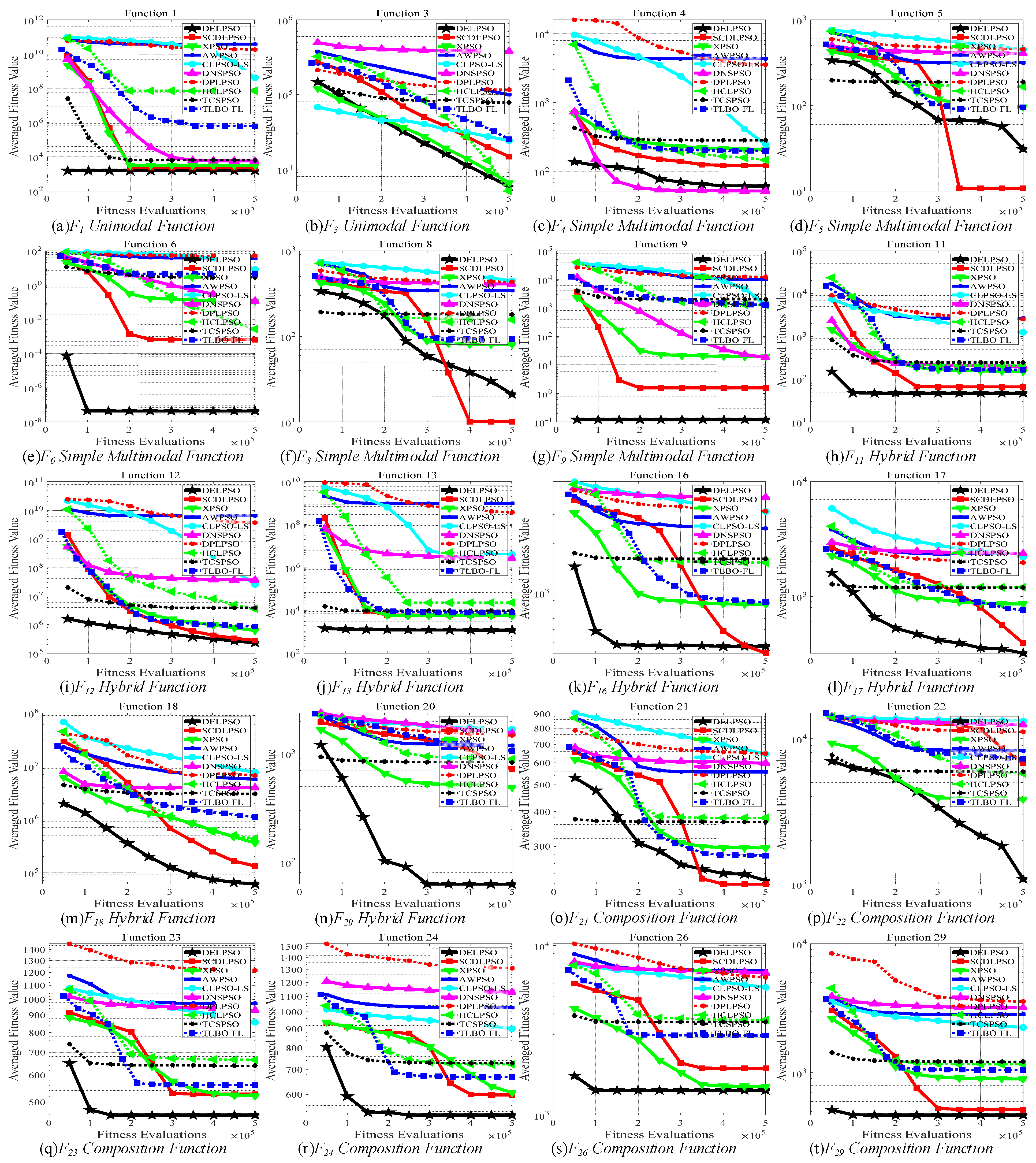
The above comparative experiments have proven the effectiveness of DELPSO with respect to the solution quality. In order to further prove its efficiency in solving complex optimization problems, experiments were carried out on the 50-D CEC 2017 benchmark set to investigate the convergence behavior comparison between the proposed DELPSO and the nine compared algorithms. Figure 1 shows the comparison results on the twenty 50-D CEC 2017 benchmark problems.
From Figure 1, the following observations can be obtained: (1) At the first look on Figure 1, we find that the proposed DELPSO achieves faster convergence speed and higher solution quality than all the nine algorithms on 16 problems. (2) In-depth observation shows that on F4, F5, F8, F16. and F21, DELPSO obtains both faster convergence speed and higher solution quality than eight compared algorithms and shows inferiority to only one compared method. (3) These two observations demonstrate the superiority of DELPSO in both the convergence speed and the solution quality, which verifies that DELPSO is efficient and effective to solve optimization problems.
To summarize, as shown in Table 5 and Figure 1, we found that the proposed DELPSO consistently shows significant superiority over most of the nine compared PSO variants on the CEC 2017 benchmark set with three dimension sizes. On the one hand, from a comprehensive point of view, the above comparative experiments verify that DELPSO maintains a good scalability when solving optimization problems. On the other hand, through the in-depth comparisons on different types of optimization problems, we found that the performance of DELPSO is significantly better than that of the compared algorithms on complicated problems, such as the multimodal problems, the hybrid problems, and the composition problems. This demonstrates that DELPSO is promising for solving complicated optimization problems. The superiority of DELPSO mainly benefits from the proposed differential elite learning strategy and the dynamic swarm partition strategy. The former selects two very different predominant particles to direct the update of each inferior one. As a result, a promising balance between fast convergence and high diversity could be maintained at the particle level. The latter strategy dynamically adjusts the number of particles in the elite group, which lets the swarm gradually change from exploring solution space to exploiting the found promising areas. As a consequence, a promising balance between exploration and exploitation at the swarm level could be maintained. With the above two techniques, the proposed DELPSO is expected to compromise search diversification and intensification well at both the particle level and the swarm level to explore and exploit the solution space properly. Therefore, DELPSO expectedly achieves promising performance in solving optimization problems.
4.3. Deep Investigation on DELPSO
In this section, we conducted extensive experiments on the 50-D CEC 2017 benchmark set, to undertake deep investigations on the proposed DELPSO. Specifically, we mainly conducted experiments to validate the effectiveness of the two main components in DELPSO, namely the proposed DEL strategy and the proposed dynamic swarm partition strategy.
4.3.1. Effectiveness of the Proposed DEL
First, we conducted experiments to investigate the effectiveness of the proposed DEL strategy. To this end, we first adopted the same roulette wheel selection strategy for the selection of the first exemplar to select the second exemplar. That is to say, better particles in EG are preferred to be selected as the two guiding exemplars. With this selection mechanism, a variant of DELPSO was developed, which we named as “DELPSO-A”. On the contrary, we also adopted the same roulette wheel selection strategy for the selection of the second exemplar to select the first exemplar. That is to say, worse particles in EG are preferred to be selected as the two guiding exemplars. With this selection mechanism, another variant of DELPSO was developed, which we named as “DELPSO-D”. At last, instead of using the devised ranking weight based roulette wheel selection strategy, we used the rankings of particles in EG to calculate the two probabilities and then select the two exemplars based the associated roulette wheel selection strategies. This variant of EDLPSO was named as “DELPSO-R”.
After the above preparation, we then conducted experiments on the 50-D CEC 2017 benchmark set to compare the four versions of DELPSO mentioned above. Table 6 shows the comparison results among the four versions of DELPSO. In this table, the best results are highlighted in bold.
From Table 6, the following observations can be obtained. (1) From the perspective of the Friedman test, the rank value of DELPSO is the smallest among the four versions of DELPSO. This demonstrates that DELPSO achieves the best overall performance. (2) Specifically, when compared with DELPSO-A and DELPSO-D, we can see that DELPSO is much better. This demonstrates that using two very different guiding exemplars based on the proposed DEL is much more effective than randomly selection of the two exemplars without considering making the two exemplars as different as possible. (3) When compared with DELPSO-R, DELPSO presents great superiority. This demonstrates the effectiveness of the probability computation as shown in Equations (6) and (8).
Based on the above observations, it was found that the proposed DEL strategy is effective and plays a key role in helping DELPSO achieve good performance.
4.3.2. Effectiveness of the Dynamic Swarm Partition Strategy
In this section, we verified the effectiveness of the proposed dynamic swarm partition strategy by adjusting the elite group size (egs) dynamically based on Equation (9). To this end, we first set egs with different fixed values by ranging from 0.2 * NP to 0.8 * NP. Then, we conducted experiments on the 50-D CEC 2017 benchmark set to compare DELPSO with the dynamic strategy and the ones with fixed values of egs. Table 7 shows the comparison results with respect to the mean fitness results over 30 independent runs. In this table, the best results are highlighted in bold.
From Table 7, the following conclusions can be drawn. (1) No matter whether it is from the perspective of the Friedman test results or in view of the number of problems where the associated algorithms achieve the best results, we can see that DELPSO with the dynamic strategy achieves much better performance than the ones with fixed settings. (2) By undertaking deep investigations, we found that the optimal setting of egs is different for different problems. Further, we found that the results obtained by DELPSO with the dynamic strategy on the problems where it does not obtain the best results are very close to the results obtained by DELPSO with the associated optimal setting of egs.
Based on the above experiments, it is verified that the dynamic partition strategy is helpful for DELPSO to achieve good performance.
5. Conclusions
This paper has proposed a differential elite learning particle swarm optimization (DELPSO) algorithm to tackle optimization problems effectively. Unlike traditional PSO variants that utilize historical best positions to direct the update of particles, DELPSO employs predominant particles in the swarm to guide the update of inferior ones. Specifically, the swarm is first dynamically divided into two groups, namely the elite group and the non-elite group, based on the devised dynamic swarm partition strategy. Then, particles in the non-elite group are updated by learning from those in the elite group, while particles in the elite group are not updated and directly enter the next generation. To let each updated particle learn from different exemplars with diverse direction, we devised two kinds of selection probabilities of particles in the elite group and then selected two very different guiding exemplars for each particle in the non-elite group. With the proposed differential elite learning strategy and the devised dynamic swarm partition strategy, the proposed DELPSO is expected to compromise exploration and exploitation well at both the swarm level and the particle level to obtain promising performance.
Extensive comparative experiments have been conducted on the widely used CEC 2017 benchmark problem set with three dimension sizes to demonstrate the effectiveness of the proposed DELPSO. By comparing with nine state-of-the-art and representative PSO variants, experimental results have demonstrated that DELPSO achieves much better performance than the compared peer algorithms. In particular, it was found that the proposed DELPSO shows particular superiority on complicated optimization problems, such as the multimodal problems, the hybrid problems, and the composition problems. At last, deep investigation on DELPSO has also been conducted to verify the effectiveness of the proposed DEL strategy and the devised dynamic swarm partition strategy.
In the future, we will apply the proposed DELPSO to solve other optimization problems, such as constrained optimization problems, multimodal optimization problems, and real-world engineering optimization problems.
Author Contributions
Q.Y.: Conceptualization, supervision, methodology, formal analysis, and writing—original draft preparation. X.G.: Implementation, formal analysis, and writing—original draft preparation. X.-D.G.: Methodology, and writing—review and editing. D.-D.X.: Methodology, and writing—review and editing. Z.-Y.L.: Writing—review and editing, and funding acquisition. All authors have read and agreed to the published version of the manuscript.
Funding
This work was supported in part by the National Natural Science Foundation of China under Grant 62006124 and U20B2061, in part by the Natural Science Foundation of Jiangsu Province under Project BK20200811, in part by the Natural Science Foundation of the Jiangsu Higher Education Institutions of China under Grant 20KJB520006, and in part by the Startup Foundation for Introducing Talent of NUIST.
Institutional Review Board Statement
Not applicable.
Informed Consent Statement
Not applicable.
Data Availability Statement
Not applicable.
Conflicts of Interest
The authors declare no conflict of interest.
References
- Eberhart, R.; Kennedy, J. A New Optimizer Using Particle Swarm Theory. In Proceedings of the Sixth International Symposium on Micro Machine and Human Science, Nagoya, Japan, 4–6 October 1995; pp. 39–43. [Google Scholar]
- Zhan, Z.H.; Shi, L.; Tan, K.C.; Zhang, J. A Survey on Evolutionary Computation for Complex Continuous Optimization. Artif. Intell. Rev. 2022, 55, 59–110. [Google Scholar] [CrossRef]
- Kundu, G.; Choudhury, S. A Discrete Genetic Learning Enabled PSO for Targeted Positive Influence Maximization in Consumer Review Networks. Innov. Syst. Softw. Eng. 2021, 17, 247–259. [Google Scholar] [CrossRef]
- Kumar, A.; Agrawal, N.; Sharma, I.; Lee, S.; Lee, H. Hilbert Transform Design Based on Fractional Derivatives and Swarm Optimization. IEEE Trans. Cybern. 2020, 50, 2311–2320. [Google Scholar] [CrossRef] [PubMed]
- Kennedy, J. Small Worlds and Mega-minds: Effects of Neighborhood Topology on Particle Swarm Performance. In Proceedings of the IEEE 1999 Congress on Evolutionary Computation, Washington, DC, USA, 6–9 July 1999; pp. 1931–1938. [Google Scholar]
- Yang, Q.; Hua, L.T.; Gao, X.D.; Xu, D.D.; Lu, Z.Y.; Jeon, S.-W.; Zhang, J. Stochastic Cognitive Dominance Leading Particle Swarm Optimization for Multimodal Problems. Mathematics 2022, 10, 761. [Google Scholar] [CrossRef]
- Li, W.; Meng, X.; Huang, Y. Differential Learning Particle Swarm Optimization with Full Dimensional Information. In Proceedings of the 2019 15th International Conference on Computational Intelligence and Security, Macao, China, 13–16 December 2019; pp. 31–35. [Google Scholar]
- Parsopoulos, K.E.; Vrahatis, M.N. On The Computation of All Global Minimizers Through Particle Swarm Optimization. IEEE Trans. Evol. Comput. 2004, 8, 211–224. [Google Scholar] [CrossRef]
- Yang, Q.; Chen, W.N.; Gu, T.; Jin, H.; Mao, W.; Zhang, J. An Adaptive Stochastic Dominant Learning Swarm Optimizer for High-Dimensional Optimization. IEEE Trans. Cybern. 2020, 52, 1960–1976. [Google Scholar] [CrossRef] [PubMed]
- Liang, J.J.; Qin, A.K.; Suganthan, P.N.; Baskar, S. Comprehensive Learning Particle Swarm Optimizer for Global Optimization of Multimodal Functions. IEEE Trans. Evol. Comput. 2006, 10, 281–295. [Google Scholar] [CrossRef]
- Meerza, S.I.A.; Islam, M.; Uzzal, M.M. Q-Learning Based Particle Swarm Optimization Algorithm for Optimal Path Planning of Swarm of Mobile Robots. In Proceedings of the 2019 1st International Conference on Advances in Science, Engineering and Robotics Technology, Dhaka, Bangladesh, 3–5 May 2019; pp. 1–5. [Google Scholar]
- Panda, A.; Ghoshal, S.; Konar, A.; Banerjee, B.; Nagar, A.K. Static Learning Particle Swarm Optimization with Enhanced Exploration and Exploitation Using Adaptive Swarm Size. In Proceedings of the 2016 IEEE Congress on Evolutionary Computation, Vancouver, BC, Canada, 24–29 July 2016; pp. 1869–1876. [Google Scholar]
- Panda, A.; Mallipeddi, R.; Das, S. Particle Swarm Optimization with A Modified Learning Strategy and Blending Crossover. In Proceedings of the 2017 IEEE Symposium Series on Computational Intelligence, Honolulu, HI, USA, 27 November–1 December 2017. [Google Scholar]
- Srimakham, S.; Jearanaitanakij, K. Improving Particle Swarm Optimization by Using Incremental Attribute Learning and Centroid of Particle’s Best Positions. In Proceedings of the 2017 14th International Conference on Electrical Engineering/Electronics, Computer, Telecommunications and Information Technology, Phuket, Thailand, 27–30 June 2017. [Google Scholar]
- Xu, G.; Zhao, X.; Wu, T.; Li, R.; Li, X. An Elitist Learning Particle Swarm Optimization With Scaling Mutation and Ring Topology. IEEE Access 2018, 6, 78453–78470. [Google Scholar] [CrossRef]
- Tang, Y.; Wei, B.; Xia, X.; Gui, L. Dynamic Multi-swarm Particle Swarm Optimization Based on Elite Learning. In Proceedings of the 2019 IEEE Symposium Series on Computational Intelligence, Xiamen, China, 6–9 December 2019; pp. 2311–2318. [Google Scholar]
- Mabaso, R.; Cleghorn, C.W. Topology-Linked Self-Adaptive Quantum Particle Swarm Optimization for Dynamic Environments. In Proceedings of the 2020 IEEE Symposium Series on Computational Intelligence, Canberra, Australia, 1–4 December 2020; pp. 1565–1572. [Google Scholar]
- Wei, L.; Fan, R.; Li, X. A Novel Multi-objective Decomposition Particle Swarm Optimization Based on Comprehensive Learning Strategy. In Proceedings of the 2017 36th the Chinese Control Conference, Dalian, China, 26–28 July 2017; pp. 2761–2766. [Google Scholar]
- Liu, S.; Lin, Q.; Li, Q.; Tan, K.C. A Comprehensive Competitive Swarm Optimizer for Large-Scale Multiobjective Optimization. IEEE Trans. Syst. Man Cybern. Syst. 2021, 1–14. [Google Scholar] [CrossRef]
- Song, W.; Hua, Z. Multi-Exemplar Particle Swarm Optimization. IEEE Access 2020, 8, 176363–176374. [Google Scholar] [CrossRef]
- Chen, Z.G.; Zhan, Z.H.; Liu, D.; Kwong, S.; Zhang, J. Particle Swarm Optimization with Hybrid Ring Topology for Multimodal Optimization Problems. In Proceedings of the 2020 IEEE International Conference on Systems, Man, and Cybernetics, Toronto, ON, Canada, 11–14 October 2020; pp. 2044–2049. [Google Scholar]
- Blackwell, T.; Kennedy, J. Impact of Communication Topology in Particle Swarm Optimization. IEEE Trans. Evol. Comput. 2019, 23, 689–702. [Google Scholar] [CrossRef] [Green Version]
- Kennedy, J.; Mendes, R. Population Structure and Particle Swarm Performance. In Proceedings of the IEEE 2002 Congress on Evolutionary Computation, Honolulu, HI, USA, 12–17 May 2002; pp. 1671–1676. [Google Scholar]
- Borowska, B. Genetic Learning Particle Swarm Optimization with Interlaced Ring Topology. In Proceedings of the Computational Science, Amsterdam, The Netherlands, 3–5 June 2020; pp. 136–148. [Google Scholar]
- Miranda, V.; Keko, H.; Jaramillo Duque, Á. Stochastic Star Communication Topology in Evolutionary Particle Swarms. Int. J. Comput. Intell. Res. 2008, 4, 105–116. [Google Scholar] [CrossRef]
- Liu, Q.; Wei, W.; Yuan, H.; Zhan, Z.-H.; Li, Y. Topology Selection for Particle Swarm Optimization. Inf. Sci. 2016, 363, 154–173. [Google Scholar] [CrossRef]
- Elsayed, S.M.; Sarker, R.A.; Essam, D.L. Memetic Multi-Topology Particle Swarm Optimizer for Constrained Optimization. In Proceedings of the 2012 IEEE Congress on Evolutionary Computation, Brisbane, Australia, 10–15 June 2012; pp. 1–8. [Google Scholar]
- Zeng, N.; Wang, Z.; Liu, W.; Zhang, H.; Hone, K.; Liu, X. A Dynamic Neighborhood-Based Switching Particle Swarm Optimization Algorithm. IEEE Trans. Cybern. 2020, 1–12. [Google Scholar] [CrossRef]
- Zhan, Z.; Zhang, J.; Li, Y.; Shi, Y. Orthogonal Learning Particle Swarm Optimization. IEEE Trans. Evol. Comput. 2011, 15, 832–847. [Google Scholar] [CrossRef] [Green Version]
- Liang, J.J.; Zhigang, S.; Zhihui, L. Coevolutionary Comprehensive Learning Particle Swarm Optimizer. In Proceedings of the IEEE Congress on Evolutionary Computation, Barcelona, Spain, 18–23 July 2010; pp. 1–8. [Google Scholar]
- Gong, Y.J.; Li, J.J.; Zhou, Y.; Li, Y.; Chung, H.S.H.; Shi, Y.H.; Zhang, J. Genetic Learning Particle Swarm Optimization. IEEE Trans. Cybern. 2016, 46, 2277–2290. [Google Scholar] [CrossRef] [Green Version]
- Yang, Q.; Chen, W.N.; Gu, T.; Zhang, H.; Yuan, H.; Kwong, S.; Zhang, J. A Distributed Swarm Optimizer With Adaptive Communication for Large-Scale Optimization. IEEE Trans. Cybern. 2020, 50, 3393–3408. [Google Scholar] [CrossRef]
- Cheng, R.; Jin, Y. A Competitive Swarm Optimizer for Large Scale Optimization. IEEE Trans. Cybern. 2015, 45, 191–204. [Google Scholar] [CrossRef]
- Cheng, R.; Jin, Y. A Social Learning Particle Swarm Optimization Algorithm for Scalable Optimization. Inf. Sci. 2015, 291, 43–60. [Google Scholar] [CrossRef]
- Yang, Q.; Chen, W.; Deng, J.D.; Li, Y.; Gu, T.; Zhang, J. A Level-Based Learning Swarm Optimizer for Large-Scale Optimization. IEEE Trans. Evol. Comput. 2018, 22, 578–594. [Google Scholar] [CrossRef]
- Yang, Q.; Chen, W.N.; Gu, T.; Zhang, H.; Deng, J.D.; Li, Y.; Zhang, J. Segment-Based Predominant Learning Swarm Optimizer for Large-Scale Optimization. IEEE Trans. Cybern. 2017, 47, 2896–2910. [Google Scholar] [CrossRef] [PubMed] [Green Version]
- Song, G.W.; Yang, Q.; Gao, X.D.; Ma, Y.Y.; Lu, Z.Y.; Zhang, J. An Adaptive Level-Based Learning Swarm Optimizer for Large-Scale Optimization. In Proceedings of the 2021 IEEE International Conference on Systems, Man, and Cybernetics, Melbourne, Australia, 17–20 October 2021; pp. 152–159. [Google Scholar]
- Wu, G.; Mallipeddi, R.; Suganthan, P. Problem Definitions and Evaluation Criteria for the CEC 2017 Competition and Special Session on Constrained Single Objective Real-Parameter Optimization; Technical Report; Nanyang Technological University: Singapore, 2016; pp. 1–16. [Google Scholar]
- Liang, J.; Ban, X.; Yu, K.; Qu, B.; Qiao, K.; Yue, C.; Chen, K.; Tan, K.C. A Survey on Evolutionary Constrained Multi-objective Optimization. IEEE Trans. Evol. Comput. 2022, 1. [Google Scholar] [CrossRef]
- Chen, K.; Zhou, F.; Liu, A. Chaotic Dynamic Weight Particle Swarm Optimization for Numerical Function Optimization. Knowl.-Based Syst. 2018, 139, 23–40. [Google Scholar] [CrossRef]
- Nickabadi, A.; Ebadzadeh, M.M.; Safabakhsh, R. A Novel Particle Swarm Optimization Algorithm with Adaptive Inertia Weight. Appl. Soft Comput. 2011, 11, 3658–3670. [Google Scholar] [CrossRef]
- Liu, W.; Wang, Z.; Yuan, Y.; Zeng, N.; Hone, K.; Liu, X. A Novel Sigmoid-Function-Based Adaptive Weighted Particle Swarm Optimizer. IEEE Trans. Cybern. 2021, 51, 1085–1093. [Google Scholar] [CrossRef]
- Xie, H.Y.; Yang, Q.; Hu, X.M.; Chen, W.N. Cross-generation Elites Guided Particle Swarm Optimization for large scale optimization. In Proceedings of the 2016 IEEE Symposium Series on Computational Intelligence, Athens, Greece, 6–9 December 2016; pp. 1–8. [Google Scholar]
- Song, A.; Chen, W.N.; Gu, T.; Zhang, H.; Zhang, J. A Constructive Particle Swarm Optimizer for Virtual Network Embedding. IEEE Trans. Netw. Sci. Eng. 2020, 7, 1406–1420. [Google Scholar] [CrossRef]
- Zhang, Y.H.; Lin, Y.; Gong, Y.J.; Zhang, J. Particle Swarm Optimization with Minimum Spanning Tree Topology for Multimodal Optimization. In Proceedings of the 2015 IEEE Symposium Series on Computational Intelligence, Cape Town, South Africa, 7–10 December 2015; pp. 234–241. [Google Scholar]
- Chen, R.M.; Huang, H.T. Particle Swarm Optimization Enhancement by Applying Global Ratio Based Communication Topology. In Proceedings of the Tenth International Conference on Intelligent Information Hiding and Multimedia Signal Processing, Kitakyushu, Japan, 27–29 August 2014; pp. 443–446. [Google Scholar]
- Lynn, N.; Suganthan, P.N. Heterogeneous Comprehensive Learning Particle Swarm Optimization with Enhanced Exploration and Exploitation. Swarm Evol. Comput. 2015, 24, 11–24. [Google Scholar] [CrossRef]
- Cao, Y.; Zhang, H.; Li, W.; Zhou, M.; Zhang, Y.; Chaovalitwongse, W.A. Comprehensive Learning Particle Swarm Optimization Algorithm With Local Search for Multimodal Functions. IEEE Trans. Evol. Comput. 2019, 23, 718–731. [Google Scholar] [CrossRef]
- Shi, Y.; Liu, H.; Gao, L.; Zhang, G. Cellular Particle Swarm Optimization. Inf. Sci. 2011, 181, 4460–4493. [Google Scholar] [CrossRef]
- Oca, M.A.M.d.; Pena, J.; Stutzle, T.; Pinciroli, C.; Dorigo, M. Heterogeneous Particle Swarm Optimizers. In Proceedings of the 2009 IEEE Congress on Evolutionary Computation, Trondheim, Norway, 18–21 May 2009; pp. 698–705. [Google Scholar]
- Engelbrecht, A.P. Scalability of A Heterogeneous Particle Swarm Optimizer. In Proceedings of the 2011 IEEE Symposium on Swarm Intelligence, Paris, France, 11–15 April 2011; pp. 1–8. [Google Scholar]
- Du, W.B.; Ying, W.; Yan, G.; Zhu, Y.B.; Cao, X.B. Heterogeneous Strategy Particle Swarm Optimization. IEEE Trans. Circuits Syst. II: Express Briefs 2017, 64, 467–471. [Google Scholar] [CrossRef] [Green Version]
- Gong, Y.-J.; Zhang, J. Small-World Particle Swarm Optimization with Topology Adaptation. In Proceedings of the 15th Annual Conference on Genetic and Evolutionary Computation, Amsterdam, The Netherlands, 6–10 July 2013; pp. 25–32. [Google Scholar]
- Lynn, N.; Suganthan, P.N. Comprehensive Learning Particle Swarm Optimizer with Guidance Vector Selection. In Proceedings of the 2013 IEEE Symposium on Swarm Intelligence, Singapore, 16–19 April 2013; pp. 80–84. [Google Scholar]
- Jin, Q.; Bin, X.; Kun, W.; Xi, Y.; Xiaoxuan, H.; Yanfei, S. Comprehensive Learning Particle Swarm Optimization with Tabu Operator Based on Ripple Neighborhood for Global Optimization. In Proceedings of the 2015 11th International Conference on Heterogeneous Networking for Quality, Reliability, Security and Robustness, Taipei, Taiwan, 19–20 August 2015; pp. 280–286. [Google Scholar]
- Yang, Q.; Chen, W.N.; Yu, Z.; Gu, T.; Li, Y.; Zhang, H.; Zhang, J. Adaptive Multimodal Continuous Ant Colony Optimization. IEEE Trans. Evol. Comput. 2017, 21, 191–205. [Google Scholar] [CrossRef] [Green Version]
- Socha, K.; Dorigo, M. Ant Colony Optimization for Continuous Domains. Eur. J. Oper. Res. 2008, 185, 1155–1173. [Google Scholar] [CrossRef] [Green Version]
- Erridge, P. The Pareto Principle. Br. Dent. J. 2006, 201, 419. [Google Scholar] [CrossRef] [PubMed] [Green Version]
- Xia, X.; Gui, L.; He, G.; Wei, B.; Zhang, Y.; Yu, F.; Wu, H.; Zhan, Z.-H. An Expanded Particle Swarm Optimization Based on Multi-Exemplar and Forgetting Ability. Inf. Sci. 2020, 508, 105–120. [Google Scholar] [CrossRef]
- Kahraman, H.T.; Aras, S.; Gedikli, E. Fitness-Distance Balance (FDB): A New Selection Method for Meta-Heuristic Search Algorithms. Knowl.-Based Syst. 2020, 190, 105169. [Google Scholar] [CrossRef]
- Zhang, X.; Liu, H.; Zhang, T.; Wang, Q.; Wang, Y.; Tu, L. Terminal Crossover and Steering-based Particle Swarm Optimization Algorithm with Disturbance. Appl. Soft Comput. 2019, 85, 105841. [Google Scholar] [CrossRef]
- Shen, Y.; Wei, L.; Zeng, C.; Chen, J. Particle Swarm Optimization with Double Learning Patterns. Comput. Intell. Neurosci. 2016, 2016, 6510303. [Google Scholar] [CrossRef] [PubMed] [Green Version]
- Kommadath, R.; Kotecha, P. Teaching Learning Based Optimization with Focused Learning and Its Performance on CEC2017 Functions. In Proceedings of the 2017 IEEE Congress on Evolutionary Computation, Donostia, Spain, 5–8 June 2017; pp. 2397–2403. [Google Scholar]
Figure 1.
Convergence behavior comparison between DELPSO and the nine compared algorithms on the twenty 50-D CEC 2017 benchmark problems.
Figure 1.
Convergence behavior comparison between DELPSO and the nine compared algorithms on the twenty 50-D CEC 2017 benchmark problems.


Table 1.
Parameters settings of all algorithms.
| Algorithms | D | Parameter Settings | |
|---|---|---|---|
| DELPSO | 30 | NP = 200 | α = 0.4 egs = 0.8 * NP~0.2 * NP |
| 50 | NP = 180 | ||
| 100 | NP = 180 | ||
| XPSO | 30 | NP = 200 | η = 0.2 p = 0.5 Stagemax = 5 |
| 50 | NP = 200 | ||
| 100 | NP = 150 | ||
| DNSPSO | 30 | NP = 50 | w = 0.9~0.4 k = 5 F = 0.5 CR = 0.9 |
| 50 | NP = 50 | ||
| 100 | NP = 50 | ||
| TCSPSO | 30 | NP = 150 | w = 0.9~0.4 c1 = c2 = 2 |
| 50 | NP = 150 | ||
| 100 | NP = 80 | ||
| CLPSO-LS | 30 | NP = 50 | c = 1.4945 w = 0.9~0.4 β = 1/3 θ = 0.94 Pc = 0.05~0.5 |
| 50 | NP = 50 | ||
| 100 | NP = 50 | ||
| AWPSO | 30 | NP = 150 | w = 0.9~0.4 b = 0.5 c = 0 d = 1.5 |
| 50 | NP = 200 | ||
| 100 | NP = 200 | ||
| DPLPSO | 30 | NP = 40 | w = 0.9~0.3 c1s = c2s = c1m = c2m = 2.0 L = 50 |
| 50 | NP = 40 | ||
| 100 | NP = 40 | ||
| HCLPSO | 30 | NP = 200 | w = 0.99~0.2 c1 = 2.5~0.5 c2 = 0.5~2.5 c = 3~1.5 |
| 50 | NP = 180 | ||
| 100 | NP = 160 | ||
| SCDLPSO | 30 | NP = 100 | w = 0.9~0.4 β = 0.5 |
| 50 | NP = 100 | ||
| 100 | NP = 150 | ||
| TLBO-FL | 30 | NP = 100 | - |
| 50 | NP = 100 | ||
| 100 | NP = 100 | ||
Table 2.
Comparison results between DELPSO and seven state-of-the-art PSO variants on the 30-D CEC 2017 benchmark functions. The symbols “+”, “−”, and “=“behind the p-values imply that DELPSO is significantly superior to, significantly inferior to, and equivalent to the compared algorithms on the relevant problems.
| F | Category | Quality | DELPSO | XPSO | DNSPSO | TCSPSO | CLPSO-LS | AWPSO | DPLPSO | HCLPSO | SCDLPSO | TLBO-FL |
|---|---|---|---|---|---|---|---|---|---|---|---|---|
| F1 | Unimodal Functions | median | 1.76 × 10³ | 2.57 × 10³ | 1.24 × 10⁵ | 1.70 × 10³ | 1.63 × 10⁴ | 7.64 × 10⁹ | 3.19 × 10⁹ | 5.49 × 10³ | 2.28 × 10³ | 2.81 × 10³ |
| mean | 2.19 × 10³ | 3.57 × 10³ | 1.58 × 10⁵ | 3.34 × 10³ | 2.01 × 10⁴ | 8.47 × 10⁹ | 3.22 × 10⁹ | 9.72 × 10³ | 3.11 × 10³ | 3.72 × 10³ | ||
| std | 2.31 × 10³ | 3.37 × 10³ | 1.33 × 10⁵ | 3.81 × 10³ | 1.08 × 10⁴ | 4.61 × 10⁹ | 1.19 × 10⁹ | 7.90 × 10³ | 3.15 × 10³ | 3.23 × 10³ | ||
| p-value | - | 7.25 × 10−2 = | 5.29 × 10⁻⁸ + | 1.68 × 10−1 = | 3.66× 10⁻¹² + | 4.55× 10⁻¹⁴ + | 4.82× 10⁻²¹ + | 7.26× 10⁻⁶ + | 2.09 × 10−1 = | 4.18× 10⁻² + | ||
| F3 | median | 3.22 × 10² | 4.32 × 101 | 1.57 × 10⁵ | 2.10 × 10⁴ | 7.68 × 10⁻¹¹ | 2.02 × 10⁴ | 3.55 × 10⁴ | 5.86 × 101 | 2.66 × 10² | 3.00 × 10³ | |
| mean | 4.16 × 10² | 6.64 × 101 | 1.54 × 10⁵ | 2.15 × 10⁴ | 1.11 × 10⁴ | 2.03 × 10⁴ | 3.70 × 10⁴ | 1.21 × 10² | 4.82 × 10² | 3.10 × 10³ | ||
| std | 3.60 × 10² | 5.70 × 101 | 2.97 × 10⁴ | 6.19 × 10³ | 2.26 × 10⁴ | 1.53 × 10⁴ | 6.91 × 10³ | 1.47 × 10² | 5.86 × 10² | 1.09 × 10³ | ||
| p-value | - | 3.09 × 10⁻⁶ − | 1.06× 10⁻³⁵ + | 9.32× 10⁻²⁶ + | 1.35× 10⁻² + | 2.92× 10⁻⁹ + | 8.25× 10−36 + | 1.36 × 10⁻⁴ − | 2.09 × 10−1 = | 2.65× 10⁻¹⁸ + | ||
| F1,3 | w/t/l | - | 0/1/1 | 2/0/0 | 1/1/0 | 2/0/0 | 2/0/0 | 2/0/0 | 1/0/1 | 0/2/0 | 2/0/0 | |
| F4 | Simple Multimodal Functions | median | 8.20 × 101 | 1.23 × 10² | 2.55 × 101 | 1.26 × 10² | 8.89 × 101 | 5.35 × 10² | 8.17 × 10² | 8.56 × 101 | 8.33 × 101 | 8.58 × 101 |
| mean | 7.60 × 101 | 1.22 × 10² | 2.55 × 101 | 1.26 × 10² | 8.93 × 101 | 8.27 × 10² | 8.51 × 10² | 8.66 × 101 | 7.66 × 101 | 8.88 × 101 | ||
| std | 9.90 × 100 | 1.23 × 101 | 9.55 × 10⁻¹ | 4.70 × 101 | 1.88 × 100 | 5.36 × 10² | 3.89 × 10² | 8.64 × 100 | 1.11 × 101 | 2.01 × 101 | ||
| p-value | - | 1.11× 10⁻²² + | 1.28 × 10⁻³⁵ − | 4.97× 10⁻⁷ + | 2.21× 10⁻⁹ + | 3.54 × 10⁻¹⁰ + | 2.13 × 10⁻¹⁵ + | 6.23 × 10⁻⁵ + | 8.53 × 10−1 = | 3.35 × 10⁻³ + | ||
| F5 | median | 8.95 × 100 | 4.03 × 101 | 1.97 × 10² | 7.32 × 101 | 2.20 × 10² | 1.44 × 10² | 2.05 × 10² | 6.31 × 101 | 4.97 × 100 | 3.52 × 101 | |
| mean | 3.42 × 101 | 4.15 × 101 | 1.97 × 10² | 7.31 × 101 | 2.19 × 10² | 1.40 × 10² | 2.02 × 10² | 6.72 × 101 | 5.14 × 100 | 3.74 × 101 | ||
| std | 5.08 × 101 | 1.20 × 101 | 1.07 × 101 | 1.97 × 101 | 9.81 × 100 | 2.75 × 101 | 2.82 × 101 | 1.63 × 101 | 1.84 × 100 | 1.80 × 101 | ||
| p-value | - | 4.53 × 10−1 = | 9.80× 10⁻²⁵ + | 2.96 × 10⁻⁴ + | 7.66× 10⁻²⁷ + | 4.28× 10⁻¹⁴ + | 2.10× 10⁻²² + | 1.48 × 10⁻³ + | 3.17 × 10⁻³ − | 7.45 × 10−1 = | ||
| F6 | median | 1.14 × 10⁻¹³ | 2.63 × 10⁻³ | 1.76 × 10⁻¹ | 1.88 × 10⁻² | 3.66 × 10⁻¹ | 1.48 × 101 | 3.02 × 101 | 3.36 × 10⁻⁴ | 1.11 × 10⁻⁶ | 3.75 × 10⁻¹ | |
| mean | 1.10 × 10⁻¹³ | 1.04 × 10⁻² | 1.83 × 10⁻¹ | 1.47 × 10⁻¹ | 4.53 × 10⁻¹ | 1.70 × 101 | 3.06 × 101 | 1.11 × 10⁻³ | 8.31 × 10⁻⁶ | 4.65 × 10⁻¹ | ||
| std | 2.04 × 10⁻¹⁴ | 2.95 × 10⁻² | 6.57 × 10⁻² | 4.12 × 10⁻¹ | 5.13 × 10⁻¹ | 7.60 × 100 | 4.93 × 100 | 1.60 × 10⁻³ | 1.41 × 10⁻⁵ | 4.07 × 10⁻¹ | ||
| p-value | - | 6.19 × 10−2 = | 9.16× 10⁻²² + | 5.90 × 10−2 = | 1.33× 10⁻⁵ + | 2.14× 10⁻¹⁷ + | 1.27 × 10−39 + | 4.11 × 10⁻⁴ + | 2.42× 10⁻³ + | 7.76× 10⁻⁸ + | ||
| F7 | median | 1.69 × 10² | 7.73 × 101 | 2.39 × 10² | 1.14 × 10² | 2.38 × 10² | 1.44 × 10² | 2.88 × 10² | 9.32 × 101 | 3.48 × 101 | 1.37 × 10² | |
| mean | 1.65 × 10² | 7.99 × 101 | 2.36 × 10² | 1.18 × 10² | 2.41 × 10² | 1.77 × 10² | 2.92 × 10² | 9.38 × 101 | 3.94 × 101 | 1.34 × 10² | ||
| std | 2.65 × 101 | 1.96 × 101 | 1.13 × 101 | 2.65 × 101 | 1.88 × 101 | 8.15 × 101 | 2.82 × 101 | 1.92 × 101 | 2.05 × 101 | 4.75 × 101 | ||
| p-value | - | 4.55 × 10⁻²⁰ − | 1.10× 10⁻¹⁹ + | 6.99 × 10⁻⁹ − | 2.56× 10⁻¹⁸ + | 4.34 × 10−1 = | 6.16× 10⁻²⁵ + | 6.83 × 10⁻¹⁷ − | 7.19 × 10⁻²⁸ − | 3.02 × 10⁻³ − | ||
| F8 | median | 8.46 × 100 | 4.03 × 101 | 2.02 × 10² | 7.51 × 101 | 2.15 × 10² | 1.39 × 10² | 1.91 × 10² | 6.47 × 101 | 3.98 × 100 | 3.04 × 101 | |
| mean | 1.72 × 101 | 4.29 × 101 | 2.00 × 10² | 8.04 × 101 | 2.15 × 10² | 1.39 × 10² | 1.91 × 10² | 6.49 × 101 | 4.58 × 100 | 3.21 × 101 | ||
| std | 3.08 × 101 | 1.29 × 101 | 1.06 × 101 | 2.46 × 101 | 1.20 × 101 | 3.06 × 101 | 2.20 × 101 | 1.84 × 101 | 1.33 × 100 | 8.44 × 100 | ||
| p-value | - | 1.12× 10⁻⁴ + | 1.01× 10−37 + | 3.06× 10⁻¹² + | 8.85× 10−39 + | 9.49× 10⁻²² + | 1.50× 10⁻³² + | 1.61× 10⁻⁹ + | 3.12 × 10⁻² − | 1.46× 10⁻² + | ||
| F9 | median | 0.00 × 100 | 9.98 × 10⁻¹ | 1.96 × 100 | 1.31 × 10² | 1.23 × 101 | 2.20 × 10³ | 1.34 × 10³ | 5.00 × 101 | 1.14 × 10⁻¹³ | 3.29 × 101 | |
| mean | 0.00 × 100 | 1.15 × 100 | 2.57 × 100 | 1.66 × 10² | 2.19 × 101 | 2.54 × 10³ | 1.42 × 10³ | 8.07 × 101 | 2.11 × 10⁻² | 3.87 × 101 | ||
| std | 0.00 × 100 | 1.00 × 100 | 2.31 × 100 | 1.73 × 10² | 3.23 × 101 | 1.40 × 10³ | 3.89 × 10² | 1.41 × 10² | 8.34 × 10⁻² | 2.94 × 101 | ||
| p-value | - | 6.67× 10⁻⁸ + | 2.59× 10⁻⁷ + | 3.00× 10⁻⁶ + | 5.84× 10⁻⁴ + | 7.69× 10⁻¹⁴ + | 2.29× 10⁻²⁷ + | 3.11× 10⁻³ + | 1.78 × 10−1 = | 2.16× 10⁻⁹ + | ||
| F10 | median | 5.68 × 10³ | 2.79 × 10³ | 5.59 × 10³ | 2.67 × 10³ | 6.20 × 10³ | 3.83 × 10³ | 6.39 × 10³ | 2.83 × 10³ | 6.32 × 10³ | 6.74 × 10³ | |
| mean | 5.13 × 10³ | 2.71 × 10³ | 5.49 × 10³ | 2.74 × 10³ | 6.11 × 10³ | 3.98 × 10³ | 6.34 × 10³ | 2.88 × 10³ | 5.97 × 10³ | 6.71 × 10³ | ||
| std | 1.77 × 10³ | 7.34 × 10² | 9.03 × 10² | 5.83 × 10² | 4.91 × 10² | 6.95 × 10² | 5.07 × 10² | 5.16 × 10² | 1.35 × 10³ | 2.65 × 10² | ||
| p-value | - | 6.27 × 10⁻⁹ − | 3.57 × 10−1 = | 4.01 × 10⁻⁹ − | 5.75× 10⁻³ + | 1.90 × 10⁻³ − | 7.85× 10⁻⁴ + | 1.45 × 10⁻⁸ − | 4.66× 10⁻² + | 1.30× 10⁻⁵ + | ||
| F4–10 | w/t/l | - | 3/2/2 | 5/1/1 | 4/1/2 | 7/0/0 | 5/1/1 | 7/0/0 | 5/0/2 | 2/2/3 | 5/1/1 | |
| F11 | Hybrid Functions | median | 1.41 × 101 | 8.70 × 101 | 8.91 × 101 | 1.12 × 10² | 1.75 × 10² | 5.96 × 10² | 3.89 × 10² | 6.80 × 101 | 1.28 × 101 | 7.90 × 101 |
| mean | 2.22 × 101 | 8.04 × 101 | 8.89 × 101 | 1.15 × 10² | 1.78 × 10² | 7.06 × 10² | 4.24 × 10² | 8.31 × 101 | 3.41 × 101 | 8.37 × 101 | ||
| std | 2.21 × 101 | 3.18 × 10+ | 9.01 × 100 | 5.90 × 101 | 4.71 × 101 | 3.55 × 10² | 1.16 × 10² | 4.33 × 101 | 2.95 × 101 | 4.43 × 101 | ||
| p-value | - | 4.18 × 10⁻¹¹ + | 2.89 × 10⁻²² + | 8.29 × 10⁻¹¹ + | 4.75 × 10⁻²³ + | 8.32 × 10⁻¹⁵ + | 9.20 × 10⁻²⁶ + | 7.50 × 10⁻⁹ + | 8.52 × 10−2 = | 9.71 × 10⁻⁹ + | ||
| F12 | median | 2.18 × 10⁴ | 2.40 × 10⁴ | 6.10 × 10⁷ | 3.87 × 10⁵ | 4.35 × 10⁵ | 2.90 × 10⁸ | 1.86 × 10⁸ | 1.86 × 10⁵ | 2.68 × 10⁴ | 3.55 × 10⁴ | |
| mean | 2.70 × 10⁴ | 1.39 × 10⁵ | 6.69 × 10⁷ | 5.47 × 10⁵ | 8.38 × 10⁵ | 4.34 × 10⁸ | 1.81 × 10⁸ | 2.81 × 10⁵ | 2.72 × 10⁴ | 4.95 × 10⁴ | ||
| std | 1.29 × 10⁴ | 3.86 × 10⁵ | 2.84 × 10⁷ | 6.21 × 10⁵ | 7.93 × 10⁵ | 5.07 × 10⁸ | 9.20 × 10⁷ | 2.59 × 10⁵ | 1.47 × 10⁴ | 7.14 × 10⁴ | ||
| p-value | - | 1.22 × 10−1 = | 2.38 × 10⁻¹⁸ + | 3.23 × 10⁻⁵ + | 8.85 × 10⁻⁷ + | 2.36 × 10⁻⁵ + | 3.64 × 10⁻¹⁵ + | 2.14 × 10⁻⁶ + | 9.74 × 10−1 = | 1.01 × 10−1 = | ||
| F13 | median | 1.06 × 10⁴ | 7.43 × 10³ | 1.45 × 10⁶ | 5.98 × 10³ | 6.55 × 10³ | 4.59 × 10⁶ | 4.97 × 10⁶ | 4.02 × 10⁴ | 8.46 × 10³ | 1.61 × 10⁴ | |
| mean | 1.12 × 10⁴ | 1.52 × 10⁴ | 1.64 × 10⁶ | 1.88 × 10⁴ | 1.38 × 10⁴ | 2.31 × 10⁷ | 1.19 × 10⁷ | 3.36 × 10⁴ | 1.80 × 10⁴ | 2.13 × 10⁴ | ||
| std | 5.69 × 10³ | 1.45 × 10⁴ | 6.42 × 10⁵ | 3.42 × 10⁴ | 1.85 × 10⁴ | 3.20 × 10⁷ | 2.24 × 10⁷ | 2.49 × 10⁴ | 1.79 × 10⁴ | 1.96 × 10⁴ | ||
| p-value | - | 1.67 × 10−1 = | 7.97 × 10⁻²⁰ + | 2.39 × 10−1 = | 4.67 × 10−1 = | 2.70 × 10⁻⁴ + | 5.80 × 10⁻³ + | 1.42 × 10⁻⁵ + | 5.38 × 10−2 = | 1.00 × 10⁻² + | ||
| F14 | median | 2.65 × 10³ | 2.97 × 10³ | 1.70 × 10² | 2.34 × 10⁴ | 9.37 × 10⁴ | 3.61 × 10⁴ | 1.19 × 10⁵ | 1.78 × 10⁴ | 1.92 × 10³ | 6.75 × 10³ | |
| mean | 3.25 × 10³ | 4.79 × 10³ | 1.76 × 10² | 4.22 × 10⁴ | 9.42 × 10⁴ | 7.51 × 10⁴ | 1.15 × 10⁵ | 2.11 × 10⁴ | 3.19 × 10³ | 7.81 × 10³ | ||
| std | 2.43 × 10³ | 5.22 × 10³ | 3.03 × 101 | 5.53 × 10⁴ | 6.01 × 10⁴ | 8.59 × 10⁴ | 9.80 × 10⁴ | 2.01 × 10⁴ | 3.20 × 10³ | 6.54 × 10³ | ||
| p-value | - | 1.57 × 10−1 = | 5.81 × 10⁻⁹ − | 3.69 × 10⁻⁴ + | 3.66 × 10⁻¹¹ + | 3.28 × 10⁻⁵ + | 7.20 × 10⁻⁸ + | 1.44 × 10⁻⁵ + | 9.36 × 10−1 = | 8.50 × 10⁻⁴ + | ||
| F15 | median | 3.18 × 10² | 5.82 × 10³ | 3.74 × 10⁴ | 8.01 × 10³ | 2.94 × 10⁴ | 9.92 × 10⁴ | 1.42 × 10⁴ | 1.13 × 10⁴ | 6.60 × 10² | 1.73 × 10⁴ | |
| mean | 1.03 × 10³ | 6.93 × 10³ | 4.17 × 10⁴ | 9.89 × 10³ | 3.15 × 10⁴ | 1.28 × 10⁵ | 2.78 × 10⁴ | 1.51 × 10⁴ | 1.70 × 10³ | 2.56 × 10⁴ | ||
| std | 1.50 × 10³ | 6.25 × 10³ | 1.70 × 10⁴ | 8.86 × 10³ | 9.88 × 10³ | 9.79 × 10⁴ | 6.34 × 10⁴ | 1.26 × 10⁴ | 2.38 × 10³ | 2.67 × 10⁴ | ||
| p-value | - | 7.02 × 10⁻⁶ + | 1.37 × 10⁻¹⁸ + | 1.81 × 10⁻⁶ + | 2.01 × 10⁻²³ + | 3.34 × 10⁻⁹ + | 2.69 × 10⁻² + | 1.73 × 10⁻⁷ + | 2.05 × 10−1 = | 7.06 × 10⁻⁶ + | ||
| F16 | median | 1.36 × 10² | 5.86 × 10² | 1.88 × 10³ | 9.22 × 10² | 1.28 × 10³ | 1.37 × 10³ | 1.57 × 10³ | 6.92 × 10² | 2.21 × 101 | 4.27 × 10² | |
| mean | 1.96 × 10² | 5.70 × 10² | 1.84 × 10³ | 9.00 × 10² | 1.10 × 10³ | 1.32 × 10³ | 1.61 × 10³ | 6.74 × 10² | 9.21 × 101 | 5.50 × 10² | ||
| std | 2.30 × 10² | 1.44 × 10² | 2.22 × 10² | 3.06 × 10² | 4.51 × 10² | 3.54 × 10² | 2.80 × 10² | 2.64 × 10² | 1.21 × 10² | 3.92 × 10² | ||
| p-value | - | 5.27 × 10⁻¹⁰ + | 3.89 × 10⁻³⁵ + | 4.35 × 10⁻¹⁴ + | 1.32 × 10⁻¹³ + | 1.11 × 10⁻²⁰ + | 7.90 × 10⁻²⁹ + | 7.17 × 10⁻¹⁰ + | 3.61 × 10⁻² − | 9.22 × 10⁻⁵ + | ||
| F17 | median | 3.46 × 101 | 1.45 × 10² | 8.28 × 10² | 3.18 × 10² | 7.31 × 10² | 5.99 × 10² | 4.96 × 10² | 2.98 × 10² | 5.11 × 101 | 1.03 × 10² | |
| mean | 4.51 × 101 | 1.37 × 10² | 8.28 × 10² | 3.30 × 10² | 1.02 × 10³ | 5.64 × 10² | 4.81 × 10² | 2.97 × 10² | 5.80 × 101 | 1.33 × 10² | ||
| std | 3.76 × 101 | 7.78 × 101 | 1.59 × 10² | 1.60 × 10² | 7.09 × 10² | 2.19 × 10² | 1.53 × 10² | 1.54 × 10² | 2.44 × 101 | 6.50 × 101 | ||
| p-value | - | 3.97 × 10⁻⁷ + | 5.09 × 10⁻²⁹ + | 3.79 × 10⁻¹³ + | 6.29 × 10⁻¹⁰ + | 2.87 × 10⁻¹⁸ + | 1.97 × 10⁻²¹ + | 6.63 × 10⁻¹² + | 1.28 × 10−1 = | 4.83 × 10⁻⁸ + | ||
| F18 | median | 9.53 × 10⁴ | 1.15 × 10⁵ | 2.04 × 10⁵ | 2.08 × 10⁵ | 6.65 × 10⁵ | 6.21 × 10⁵ | 5.81 × 10⁵ | 1.58 × 10⁵ | 8.54 × 10⁴ | 3.52 × 10⁵ | |
| mean | 1.03 × 10⁵ | 1.37 × 10⁵ | 2.08 × 10⁵ | 3.19 × 10⁵ | 2.18 × 10⁶ | 1.63 × 10⁶ | 1.04 × 10⁶ | 2.01 × 10⁵ | 1.16 × 10⁵ | 3.86 × 10⁵ | ||
| std | 5.13 × 10⁴ | 8.19 × 10⁴ | 8.98 × 10⁴ | 2.64 × 10⁵ | 2.84 × 10⁶ | 2.81 × 10⁶ | 1.18 × 10⁶ | 1.24 × 10⁵ | 9.74 × 10⁴ | 1.81 × 10⁵ | ||
| p-value | - | 6.40 × 10−2 = | 9.45 × 10⁻⁷ + | 5.93 × 10⁻⁵ + | 2.24 × 10⁻⁴ + | 4.80 × 10⁻³ + | 7.08 × 10⁻⁵ + | 2.41 × 10⁻⁴ + | 5.21 × 10−1 = | 4.28 × 10⁻¹¹ + | ||
| F19 | median | 2.74 × 10³ | 2.32 × 10³ | 2.06 × 10³ | 9.93 × 10³ | 1.57 × 10⁴ | 1.16 × 10⁶ | 1.52 × 10⁴ | 1.07 × 10⁴ | 1.72 × 10³ | 6.75 × 10³ | |
| mean | 3.34 × 10³ | 3.67 × 10³ | 2.44 × 10³ | 1.31 × 10⁴ | 2.49 × 10⁶ | 2.35 × 10⁷ | 2.95 × 10⁴ | 1.77 × 10⁴ | 3.58 × 10³ | 1.18 × 10⁴ | ||
| std | 2.49 × 10³ | 3.04 × 10³ | 1.28 × 10³ | 1.25 × 10⁴ | 1.33 × 10⁷ | 4.77 × 10⁷ | 5.66 × 10⁴ | 1.99 × 10⁴ | 3.83 × 10³ | 1.30 × 10⁴ | ||
| p-value | - | 6.59 × 10−1 = | 8.63 × 10−2 = | 5.33 × 10⁻⁵ + | 3.17 × 10−1 = | 1.02 × 10⁻² + | 1.57 × 10⁻² + | 2.97 × 10⁻⁴ + | 7.75 × 10−1 = | 1.01 × 10⁻³ + | ||
| F20 | median | 1.42 × 10² | 1.74 × 10² | 3.64 × 10² | 3.31 × 10² | 5.75 × 10² | 4.28 × 10² | 3.75 × 10² | 1.78 × 10² | 4.23 × 101 | 2.16 × 10² | |
| mean | 1.16 × 10² | 1.86 × 10² | 3.95 × 10² | 3.44 × 10² | 5.18 × 10² | 4.37 × 10² | 3.95 × 10² | 1.89 × 10² | 6.38 × 101 | 2.27 × 10² | ||
| std | 4.69 × 101 | 5.72 × 101 | 1.84 × 10² | 1.18 × 10² | 1.90 × 10² | 1.80 × 10² | 1.24 × 10² | 1.18 × 10² | 7.20 × 101 | 1.11 × 10² | ||
| p-value | - | 4.98 × 10⁻⁶ + | 8.70 × 10⁻¹¹ + | 1.23 × 10⁻¹³ + | 6.52 × 10⁻¹⁶ + | 5.01 × 10⁻¹³ + | 2.51 × 10⁻¹⁶ + | 3.21 × 10⁻³ + | 1.64 × 10⁻³ − | 6.19 × 10⁻⁶ + | ||
| F11–20 | w/t/l | - | 5/5/0 | 8/1/1 | 9/1/0 | 8/2/0 | 10/0/0 | 10/0/0 | 10/0/0 | 0/8/2 | 9/1/0 | |
| F21 | Composition Functions | median | 2.09 × 10² | 2.42 × 10² | 3.99 × 10² | 2.77 × 10² | 4.06 × 10² | 3.44 × 10² | 4.09 × 10² | 2.73 × 10² | 2.09 × 10² | 2.34 × 10² |
| mean | 2.24 × 10² | 2.43 × 10² | 3.99 × 10² | 2.83 × 10² | 4.04 × 10² | 3.53 × 10² | 4.05 × 10² | 2.72 × 10² | 2.09 × 10² | 2.34 × 10² | ||
| std | 3.93 × 101 | 1.23 × 101 | 1.11 × 101 | 2.02 × 101 | 9.77 × 100 | 3.66 × 101 | 2.10 × 101 | 1.53 × 101 | 2.82 × 100 | 1.06 × 101 | ||
| p-value | - | 1.63 × 10⁻² + | 8.00 × 10⁻³¹ + | 1.96 × 10⁻⁹ + | 1.17 × 10⁻³¹ + | 1.20 × 10⁻¹⁸ + | 1.22 × 10⁻²⁹ + | 8.06 × 10⁻⁸ + | 4.85 × 10⁻² - | 1.81 × 10−1 = | ||
| F22 | median | 1.00 × 10² | 1.00 × 10² | 6.45 × 10³ | 1.00 × 10² | 7.00 × 10³ | 3.90 × 10³ | 5.41 × 10² | 1.00 × 10² | 1.00 × 10² | 1.00 × 10² | |
| m × 10an | 1.00 × 10² | 2.40 × 10² | 6.28 × 10³ | 1.04 × 10³ | 6.98 × 10³ | 3.36 × 10³ | 5.63 × 10² | 1.88 × 10² | 2.73 × 10² | 1.01 × 10² | ||
| std | 0.00 × 100 | 5.29 × 10² | 6.67 × 10² | 1.46 × 10³ | 3.01 × 10² | 1.28 × 10³ | 1.30 × 10² | 4.72 × 10² | 9.33 × 10² | 1.47 × 100 | ||
| p-value | - | 1.61 × 10−1 = | 2.30 × 10−49 + | 9.84 × 10⁻⁴ + | 7.93 × 10−72 + | 7.66 × 10⁻²⁰ + | 8.89 × 10⁻²⁷ + | 3.17 × 10−1 = | 3.21 × 10−1 = | 2.82 × 10⁻³ + | ||
| F23 | median | 3.63 × 10² | 3.91 × 10² | 5.74 × 10² | 4.41 × 10² | 5.56 × 10² | 5.60 × 10² | 6.77 × 10² | 4.49 × 10² | 3.92 × 10² | 3.92 × 10² | |
| mean | 3.63 × 10² | 3.93 × 10² | 5.86 × 10² | 4.43 × 10² | 5.54 × 10² | 5.63 × 10² | 6.85 × 10² | 4.51 × 10² | 3.91 × 10² | 3.96 × 10² | ||
| std | 4.89 × 100 | 1.34 × 101 | 4.21 × 101 | 3.10 × 101 | 1.14 × 101 | 4.09 × 101 | 3.69 × 101 | 1.97 × 101 | 9.71 × 100 | 1.51 × 101 | ||
| p-value | - | 7.10 × 10⁻¹⁶ + | 1.27 × 10⁻³⁵ + | 9.05 × 10⁻²⁰ + | 6.78 × 10−62 + | 8.34 × 10⁻³⁴ + | 1.19 × 10−47 + | 5.27 × 10⁻³¹ + | 8.69 × 10⁻²⁰ + | 1.08 × 10⁻¹⁵ + | ||
| F24 | median | 4.32 × 10² | 4.56 × 10² | 6.61 × 10² | 5.04 × 10² | 6.21 × 10² | 6.48 × 10² | 7.31 × 10² | 5.38 × 10² | 4.66 × 10² | 4.64 × 10² | |
| mean | 4.32 × 10² | 4.58 × 10² | 6.73 × 10² | 5.19 × 10² | 6.22 × 10² | 6.52 × 10² | 7.35 × 10² | 5.41 × 10² | 4.70 × 10² | 4.68 × 10² | ||
| std | 3.12 × 100 | 1.23 × 101 | 4.38 × 101 | 4.73 × 101 | 1.14 × 101 | 3.91 × 101 | 4.60 × 101 | 2.46 × 101 | 1.60 × 101 | 1.57 × 101 | ||
| p-value | - | 8.36 × 10⁻¹⁶ + | 1.17 × 10−36 + | 5.08 × 10⁻¹⁴ + | 5.57 × 10−63 + | 4.29 × 10−37 + | 6.94 × 10−41 + | 2.05 × 10⁻³¹ + | 4.49 × 10⁻¹⁸ + | 4.17 × 10⁻¹⁷ + | ||
| F25 | median | 3.88 × 10² | 3.91 × 10² | 3.79 × 10² | 4.16 × 10² | 3.88 × 10² | 5.41 × 10² | 5.86 × 10² | 3.89 × 10² | 3.88 × 10² | 3.95 × 10² | |
| mean | 3.88 × 10² | 3.93 × 10² | 3.78 × 10² | 4.13 × 10² | 3.88 × 10² | 6.37 × 10² | 6.06 × 10² | 3.89 × 10² | 3.88 × 10² | 4.03 × 10² | ||
| std | 3.98 × 10⁻¹ | 6.41 × 100 | 6.16 × 10⁻¹ | 2.16 × 101 | 1.28 × 10⁻¹ | 1.95 × 10² | 6.43 × 101 | 6.58 × 100 | 5.00 × 10⁻¹ | 1.62 × 101 | ||
| p-value | - | 2.90 × 10⁻⁵ + | 2.98 × 10−51 - | 2.62 × 10⁻⁸ + | NAN = | 4.17 × 10⁻⁹ + | 1.07 × 10⁻²⁵ + | 1.29 × 10−1 = | 9.79 × 10−1 = | 3.98 × 10⁻⁶ + | ||
| F26 | median | 1.09 × 10³ | 3.00 × 10² | 3.20 × 10³ | 2.05 × 10³ | 3.18 × 10³ | 3.27 × 10³ | 1.62 × 10³ | 1.93 × 10³ | 1.33 × 10³ | 1.48 × 10³ | |
| mean | 1.07 × 10³ | 5.95 × 10² | 3.27 × 10³ | 2.02 × 10³ | 3.16 × 10³ | 3.23 × 10³ | 2.21 × 10³ | 1.77 × 10³ | 1.33 × 10³ | 1.39 × 10³ | ||
| std | 1.60 × 10² | 5.28 × 10² | 3.88 × 10² | 4.75 × 10² | 1.19 × 10² | 6.87 × 10² | 1.16 × 10³ | 6.07 × 10² | 1.15 × 10² | 4.67 × 10² | ||
| p-value | - | 2.06 × 10⁻⁵ - | 1.57 × 10⁻³⁵ + | 1.40 × 10⁻¹⁴ + | 1.93 × 10−52 + | 1.45 × 10⁻²³ + | 2.53 × 10⁻⁶ + | 1.35 × 10⁻⁷ + | 1.45 × 10⁻⁹ + | 9.01 × 10⁻⁴ + | ||
| F27 | median | 5.10 × 10² | 5.36 × 10² | 5.00 × 10² | 5.63 × 10² | 5.12 × 10² | 5.85 × 10² | 7.96 × 10² | 5.13 × 10² | 5.14 × 10² | 5.33 × 10² | |
| mean | 5.12 × 10² | 5.37 × 10² | 5.00 × 10² | 5.64 × 10² | 5.18 × 10² | 6.02 × 10² | 8.01 × 10² | 5.15 × 10² | 5.15 × 10² | 5.34 × 10² | ||
| std | 8.45 × 100 | 1.68 × 101 | 7.67 × 10⁻⁵ | 1.99 × 101 | 1.48 × 101 | 5.52 × 101 | 4.09 × 101 | 1.40 × 101 | 9.77 × 100 | 2.08 × 101 | ||
| p-value | - | 1.65 × 10⁻⁹ + | 1.90 × 10⁻¹⁰ - | 1.13 × 10⁻¹⁸ + | 5.10 × 10−2 = | 5.05 × 10⁻¹² + | 3.46 × 10−42 + | 3.03 × 10−1 = | 1.82 × 10−1 = | 2.10 × 10⁻⁶ + | ||
| F28 | median | 3.17 × 10² | 4.04 × 10² | 5.00 × 10² | 4.28 × 10² | 3.52 × 10³ | 9.04 × 10² | 8.91 × 10² | 4.45 × 10² | 4.08 × 10² | 4.24 × 10² | |
| mean | 3.44 × 10² | 3.84 × 10² | 5.00 × 10² | 4.49 × 10² | 3.00 × 10³ | 1.24 × 10³ | 9.21 × 10² | 4.49 × 10² | 4.15 × 10² | 4.30 × 10² | ||
| std | 4.93 × 101 | 6.17 × 101 | 7.50 × 10⁻⁵ | 5.53 × 101 | 9.61 × 10² | 7.22 × 10² | 1.46 × 10² | 3.77 × 101 | 3.61 × 101 | 2.52 × 101 | ||
| p-value | - | 8.41 × 10⁻³ + | 3.09 × 10⁻²⁴ + | 2.81 × 10⁻¹⁰ + | 1.99 × 10⁻²¹ + | 1.06 × 10⁻⁸ + | 6.68 × 10⁻²⁸ + | 1.03 × 10⁻¹² + | 5.79 × 10⁻⁸ + | 1.47 × 10⁻¹¹ + | ||
| F29 | median | 4.34 × 10² | 5.39 × 10² | 1.72 × 10³ | 8.34 × 10² | 9.84 × 10² | 1.10 × 10³ | 1.22 × 10³ | 6.50 × 10² | 4.80 × 10² | 5.88 × 10² | |
| mean | 4.46 × 10² | 5.50 × 10² | 1.67 × 10³ | 8.19 × 10² | 1.08 × 10³ | 1.11 × 10³ | 1.28 × 10³ | 7.08 × 10² | 4.80 × 10² | 6.19 × 10² | ||
| std | 4.30 × 101 | 7.92 × 101 | 2.74 × 10² | 1.72 × 10² | 5.52 × 10² | 2.96 × 10² | 2.19 × 10² | 2.01 × 10² | 2.24 × 101 | 9.51 × 101 | ||
| p-value | - | 6.02 × 10⁻⁸ + | 1.75 × 10⁻³¹ + | 2.36 × 10⁻¹⁶ + | 6.78 × 10⁻⁸ + | 2.72 × 10⁻¹⁷ + | 7.08 × 10⁻²⁸ + | 4.98 × 10⁻⁹ + | 3.84 × 10⁻⁴ + | 1.87 × 10⁻¹² + | ||
| F30 | median | 3.33 × 10³ | 7.33 × 10³ | 5.18 × 10⁴ | 1.15 × 10⁴ | 1.38 × 10⁴ | 1.39 × 10⁶ | 1.86 × 10⁶ | 6.27 × 10³ | 3.90 × 10³ | 1.57 × 10⁴ | |
| mean | 3.63 × 10³ | 8.63 × 10³ | 5.96 × 10⁴ | 1.55 × 10⁴ | 1.38 × 10⁴ | 2.79 × 10⁶ | 3.35 × 10⁶ | 8.22 × 10³ | 5.05 × 10³ | 2.93 × 10⁴ | ||
| std | 9.10 × 10² | 4.01 × 10³ | 3.90 × 10⁴ | 1.30 × 10⁴ | 1.36 × 10³ | 3.17 × 10⁶ | 3.00 × 10⁶ | 5.02 × 10³ | 2.81 × 10³ | 3.45 × 10⁴ | ||
| p-value | - | 1.71 × 10⁻⁸ + | 1.79 × 10⁻¹⁰ + | 7.93 × 10⁻⁶ + | 1.35 × 10−39 + | 1.45 × 10⁻⁵ + | 1.28 × 10⁻⁷ + | 9.64 × 10⁻⁶ + | 1.18 × 10⁻² + | 1.77 × 10⁻⁴ + | ||
| F21–30 | w/t/l | - | 8/1/1 | 8/0/2 | 10/0/0 | 8/2/0 | 10/0/0 | 10/0/0 | 7/3/0 | 6/3/1 | 9/1/0 | |
| w/t/l | - | 16/9/4 | 23/2/4 | 24/3/2 | 25/4/0 | 27/1/1 | 29/0/0 | 23/3/3 | 8/15/6 | 25/3/1 | ||
| Rank | 1.79 | 3.48 | 6.76 | 5.93 | 7.59 | 8.52 | 8.83 | 4.72 | 2.48 | 4.90 | ||
Table 3.
Comparison results between DELPSO and seven state-of-the-art PSO variants on the 50-D CEC 2017 benchmark functions. The symbols “+”, “−”, and “=“behind the p-values imply that DELPSO is significantly superior to, significantly inferior to, and equivalent to the compared algorithms on the relevant problems.
| F | Category | Quality | DELPSO | XPSO | DNSPSO | TCSPSO | CLPSO-LS | AWPSO | DPLPSO | HCLSPO | SCDLPSO | TLBO-FL |
|---|---|---|---|---|---|---|---|---|---|---|---|---|
| F1 | Unimodal Functions | median | 1.46 × 10³ | 1.99 × 10³ | 1.72 × 10³ | 3.79 × 10³ | 4.97 × 10⁷ | 3.84 × 10¹⁰ | 1.86 × 10¹⁰ | 9.83 × 10³ | 1.01 × 10³ | 1.77 × 10⁴ |
| mean | 2.86 × 10³ | 3.17 × 10³ | 5.68 × 10³ | 6.30 × 10³ | 3.73 × 10⁸ | 3.81 × 10¹⁰ | 1.82 × 10¹⁰ | 7.17 × 10⁷ | 2.32 × 10³ | 6.09 × 10⁵ | ||
| std | 3.17 × 10³ | 3.47 × 10³ | 7.60 × 10³ | 6.91 × 10³ | 1.34 × 10⁹ | 7.86 × 10⁹ | 4.26 × 10⁹ | 2.73 × 10⁸ | 2.71 × 10³ | 2.49 × 10⁶ | ||
| p-value | - | 2.68 × 10⁻² + | 5.88 × 10⁻³ + | 1.65 × 10−1 = | 1.40 × 10−1 = | 1.01 × 10⁻³³ + | 8.00 × 10⁻³¹ + | 1.63 × 10−1 = | 1.93 × 10−1 = | 1.95 × 10−1 = | ||
| F3 | median | 6.00 × 10³ | 6.14 × 10³ | 3.80 × 10⁵ | 7.83 × 10⁴ | 5.36 × 10⁻¹⁰ | 9.79 × 10⁴ | 1.16 × 10⁵ | 4.71 × 10³ | 1.38 × 10⁴ | 2.43 × 10⁴ | |
| mean | 6.46 × 10³ | 6.56 × 10³ | 3.79 × 10⁵ | 7.79 × 10⁴ | 1.52 × 10⁴ | 9.87 × 10⁴ | 1.16 × 10⁵ | 5.11 × 10³ | 1.44 × 10⁴ | 2.53 × 10⁴ | ||
| std | 1.98 × 10³ | 2.57 × 10³ | 3.68 × 10⁴ | 1.21 × 10⁴ | 4.57 × 10⁴ | 2.62 × 10⁴ | 1.82 × 10⁴ | 2.40 × 10³ | 3.94 × 10³ | 4.79 × 10³ | ||
| p-value | - | 2.41 × 10−1 = | 1.65 × 10−51 + | 1.50 × 10−39 + | 2.75 × 10−1 = | 6.46 × 10⁻²⁸ + | 8.84 × 10−39 + | 1.92 × 10−1 = | 4.79 × 10⁻¹⁵ + | 4.55 × 10⁻²⁸ + | ||
| F1,3 | w/t/l | - | 1/1/0 | 2/0/0 | 1/1/0 | 0/2/0 | 2/0/0 | 2/0/0 | 0/2/0 | 1/1/0 | 1/1/0 | |
| F4 | Simple Multimodal Functions | median | 2.85 × 101 | 2.14 × 10² | 4.56 × 101 | 2.90 × 10² | 2.40 × 10² | 2.97 × 10³ | 3.55 × 10³ | 1.61 × 10² | 1.33 × 10² | 2.18 × 10² |
| mean | 5.65 × 101 | 2.10 × 10² | 5.25 × 101 | 2.86 × 10² | 2.39 × 10² | 4.33 × 10³ | 3.55 × 10³ | 1.48 × 10² | 1.23 × 10² | 2.00 × 10² | ||
| std | 3.96 × 101 | 5.38 × 101 | 1.80 × 101 | 7.76 × 101 | 9.77 × 100 | 2.53 × 10³ | 8.41 × 10² | 5.23 × 101 | 5.20 × 101 | 4.52 × 101 | ||
| p-value | - | 4.04 × 10⁻¹⁶ + | 3.09 × 10−1 = | 7.71 × 10⁻¹⁸ + | 8.41 × 10⁻²⁸ + | 1.09 × 10⁻¹² + | 4.03 × 10⁻³⁰ + | 1.28 × 10⁻⁸ + | 1.70 × 10⁻⁵ + | 1.76 × 10⁻¹⁶ + | ||
| F5 | median | 1.94 × 101 | 9.25 × 101 | 4.10 × 10² | 1.87 × 10² | 4.47 × 10² | 3.11 × 10² | 4.61 × 10² | 1.65 × 10² | 1.04 × 101 | 9.65 × 101 | |
| mean | 2.65 × 101 | 9.59 × 101 | 4.06 × 10² | 1.88 × 10² | 4.47 × 10² | 3.15 × 10² | 4.55 × 10² | 1.66 × 10² | 1.08 × 101 | 9.52 × 101 | ||
| std | 3.59 × 101 | 2.36 × 101 | 2.60 × 101 | 4.08 × 101 | 1.31 × 101 | 4.96 × 101 | 3.04 × 101 | 3.23 × 101 | 3.61 × 100 | 1.60 × 101 | ||
| p-value | - | 5.62 × 10⁻⁹ + | 4.60 × 10−43 + | 1.99 × 10⁻¹⁸ + | 3.79 × 10−48 + | 4.64 × 10⁻²⁹ + | 5.35 × 10−45 + | 6.78 × 10⁻¹⁹ + | 1.97 × 10⁻² − | 1.39 × 10⁻⁹ + | ||
| F6 | median | 1.14 × 10⁻¹³ | 6.53 × 10⁻² | 1.03 × 10⁻¹ | 2.04 × 100 | 6.61 × 100 | 3.65 × 101 | 5.06 × 101 | 1.85 × 10⁻³ | 5.14 × 10⁻⁴ | 4.43 × 100 | |
| mean | 3.52 × 10⁻⁸ | 1.14 × 10⁻¹ | 1.14 × 10⁻¹ | 2.82 × 100 | 6.96 × 100 | 3.79 × 101 | 5.02 × 101 | 2.65 × 10⁻³ | 6.37 × 10⁻⁴ | 4.51 × 100 | ||
| std | 1.15 × 10⁻⁷ | 1.42 × 10⁻¹ | 4.30 × 10⁻² | 2.67 × 100 | 1.66 × 100 | 7.15 × 100 | 4.23 × 100 | 2.37 × 10⁻³ | 5.24 × 10⁻⁴ | 1.76 × 100 | ||
| p-value | - | 6.06 × 10⁻⁵ + | 1.22 × 10⁻²⁰ + | 6.40 × 10⁻⁸ + | 2.18 × 10⁻³⁰ + | 8.42 × 10−36 + | 1.70 × 10−55 + | 1.24 × 10⁻⁷ + | 1.64 × 10⁻⁸ + | 5.22 × 10⁻²⁰ + | ||
| F7 | median | 3.40 × 10² | 1.41 × 10² | 4.67 × 10² | 2.98 × 10² | 5.06 × 10² | 6.87 × 10² | 7.56 × 10² | 1.94 × 10² | 6.18 × 101 | 1.75 × 10² | |
| mean | 3.26 × 10² | 1.47 × 10² | 4.66 × 10² | 2.91 × 10² | 5.07 × 10² | 6.94 × 10² | 7.61 × 10² | 2.02 × 10² | 6.22 × 101 | 1.77 × 10² | ||
| std | 5.19 × 101 | 2.36 × 101 | 1.69 × 101 | 4.53 × 101 | 3.91 × 101 | 1.95 × 10² | 6.56 × 101 | 3.06 × 101 | 2.31 × 100 | 4.21 × 101 | ||
| p-value | - | 6.62 × 10⁻¹¹ − | 1.03 × 10⁻¹³ + | 7.17 × 10−1 = | 3.56 × 10⁻¹⁶ + | 6.88 × 10⁻²¹ + | 1.16 × 10⁻²⁹ + | 9.74 × 10⁻⁶ − | 8.03 × 10⁻¹⁹ − | 1.77 × 10⁻⁷ − | ||
| F8 | median | 1.89 × 101 | 7.71 × 101 | 4.05 × 10² | 1.76 × 10² | 4.40 × 10² | 3.47 × 10² | 4.35 × 10² | 1.56 × 10² | 9.45 × 100 | 8.66 × 101 | |
| mean | 5.54 × 101 | 8.07 × 101 | 4.11 × 10² | 1.80 × 10² | 4.40 × 10² | 3.44 × 10² | 4.33 × 10² | 1.56 × 10² | 1.01 × 101 | 9.28 × 101 | ||
| std | 8.62 × 101 | 1.93 × 101 | 1.83 × 101 | 4.21 × 101 | 1.81 × 101 | 5.59 × 101 | 2.37 × 101 | 2.67 × 101 | 3.34 × 100 | 1.51 × 101 | ||
| p-value | - | 2.37 × 10⁻²³ + | 3.55 × 10−96 + | 7.62 × 10⁻²³ + | 1.14 × 10−71 + | 5.42 × 10⁻³⁵ + | 1.02 × 10−64 + | 1.43 × 10⁻³⁴ + | 6.55 × 10⁻¹⁷ − | 1.48 × 10⁻³² + | ||
| F9 | median | 1.14 × 10⁻¹³ | 1.13 × 101 | 1.14 × 101 | 1.72 × 10³ | 9.87 × 10² | 9.41 × 10³ | 1.15 × 10⁴ | 1.25 × 10³ | 5.89 × 10⁻¹ | 7.96 × 10² | |
| mean | 2.11 × 10⁻² | 1.96 × 101 | 1.69 × 101 | 1.98 × 10³ | 1.05 × 10³ | 9.96 × 10³ | 1.21 × 10⁴ | 1.26 × 10³ | 1.57 × 100 | 1.28 × 10³ | ||
| std | 8.35 × 10⁻² | 3.02 × 101 | 2.48 × 101 | 1.09 × 10³ | 3.18 × 10² | 4.02 × 10³ | 2.22 × 10³ | 5.35 × 10² | 3.67 × 100 | 1.12 × 10³ | ||
| p-value | - | 9.62 × 10⁻⁴ + | 5.95 × 10⁻⁴ + | 4.85 × 10⁻¹⁰ + | 4.03 × 10⁻²⁵ + | 2.42 × 10⁻¹⁹ + | 1.52 × 10−36 + | 2.26 × 10⁻¹⁸ + | 3.80 × 10⁻² + | 7.55 × 10⁻⁸ + | ||
| F10 | median | 1.05 × 10⁴ | 5.17 × 10³ | 1.13 × 10⁴ | 5.62 × 10³ | 1.32 × 10⁴ | 8.09 × 10³ | 1.24 × 10⁴ | 5.58 × 10³ | 1.20 × 10⁴ | 1.27 × 10⁴ | |
| mean | 8.27 × 10³ | 5.20 × 10³ | 1.13 × 10⁴ | 5.61 × 10³ | 1.31 × 10⁴ | 7.57 × 10³ | 1.24 × 10⁴ | 5.57 × 10³ | 9.87 × 10³ | 1.26 × 10⁴ | ||
| std | 4.48 × 10³ | 7.20 × 10² | 1.17 × 10³ | 9.05 × 10² | 4.43 × 10² | 1.26 × 10³ | 6.48 × 10² | 6.11 × 10² | 3.77 × 10³ | 4.32 × 10² | ||
| p-value | - | 7.92 × 10−2 = | 7.63 × 10⁻⁶ + | 1.43 × 10−1 = | 2.17 × 10⁻⁹ + | 1.07 × 10⁻⁷ − | 5.72 × 10⁻⁸ + | 1.75 × 10−1 = | 8.85 × 10⁻³ + | 1.75 × 10⁻⁸ + | ||
| F4–10 | w/t/l | - | 5/1/1 | 6/1/0 | 5/2/0 | 7/0/0 | 6/0/1 | 7/0/0 | 5/1/1 | 4/0/3 | 6/0/1 | |
| F11 | Hybrid Functions | median | 4.16 × 101 | 1.56 × 10² | 2.01 × 10² | 2.37 × 10² | 2.75 × 10² | 1.44 × 10³ | 2.45 × 10³ | 2.08 × 10² | 6.05 × 101 | 1.68 × 10² |
| mean | 4.20 × 101 | 1.51 × 10² | 2.00 × 10² | 2.45 × 10² | 2.71 × 10² | 2.66 × 10³ | 2.55 × 10³ | 2.07 × 10² | 6.61 × 101 | 1.67 × 10² | ||
| std | 9.17 × 100 | 3.32 × 101 | 1.66 × 101 | 1.02 × 10² | 7.06 × 101 | 2.26 × 10³ | 7.55 × 10² | 6.30 × 101 | 1.85 × 101 | 4.80 × 101 | ||
| p-value | - | 4.53 × 10⁻²³ + | 1.11 × 10−45 + | 8.92 × 10⁻¹³ + | 4.31 × 10⁻²⁴ + | 4.42 × 10⁻⁸ + | 2.99 × 10⁻²⁵ + | 1.40 × 10⁻¹⁹ + | 8.60 × 10⁻⁶ + | 5.13 × 10⁻¹⁹ + | ||
| F12 | median | 2.09 × 10⁵ | 3.27 × 10⁵ | 3.05 × 10⁷ | 2.45 × 10⁶ | 2.02 × 10⁷ | 5.67 × 10⁹ | 3.43 × 10⁹ | 2.94 × 10⁶ | 2.22 × 10⁵ | 6.12 × 10⁵ | |
| mean | 2.29 × 10⁵ | 6.22 × 10⁵ | 3.60 × 10⁷ | 3.89 × 10⁶ | 2.37 × 10⁷ | 6.39 × 10⁹ | 3.65 × 10⁹ | 3.61 × 10⁶ | 2.78 × 10⁵ | 8.59 × 10⁵ | ||
| std | 1.00 × 10⁵ | 8.04 × 10⁵ | 2.33 × 10⁷ | 5.41 × 10⁶ | 1.20 × 10⁷ | 2.91 × 10⁹ | 1.16 × 10⁹ | 2.48 × 10⁶ | 1.61 × 10⁵ | 9.08 × 10⁵ | ||
| p-value | - | 1.18 × 10⁻² + | 2.05 × 10⁻¹⁵ + | 1.92 × 10⁻⁹ + | 4.07 × 10⁻¹⁵ + | 4.53 × 10⁻¹⁷ + | 3.63 × 10⁻²⁴ + | 7.90 × 10⁻¹⁰ + | 1.91 × 10−1 = | 4.77 × 10⁻⁴ + | ||
| F13 | median | 1.12 × 10³ | 3.06 × 10³ | 2.02 × 10⁶ | 7.19 × 10³ | 3.78 × 10⁴ | 6.36 × 10⁸ | 3.74 × 10⁸ | 2.14 × 10⁴ | 3.29 × 10³ | 6.37 × 10³ | |
| mean | 2.61 × 10³ | 5.58 × 10³ | 2.59 × 10⁶ | 9.61 × 10³ | 4.00 × 10⁶ | 9.74 × 10⁸ | 3.68 × 10⁸ | 2.29 × 10⁴ | 5.90 × 10³ | 7.86 × 10³ | ||
| std | 4.15 × 10³ | 5.99 × 10³ | 1.78 × 10⁶ | 8.94 × 10³ | 1.01 × 10⁷ | 1.22 × 10⁹ | 2.55 × 10⁸ | 1.32 × 10⁴ | 6.31 × 10³ | 4.11 × 10³ | ||
| p-value | - | 4.04 × 10⁻⁴ + | 1.22 × 10⁻¹⁰ + | 8.43 × 10⁻⁶ + | 3.75 × 10⁻² + | 6.92 × 10⁻⁵ + | 1.48 × 10⁻¹⁰ + | 2.76 × 10⁻¹² + | 3.06 × 10⁻⁴ + | 7.83 × 10⁻¹¹ + | ||
| F14 | median | 2.35 × 10⁴ | 3.05 × 10⁴ | 7.46 × 10³ | 7.62 × 10⁴ | 2.69 × 10⁵ | 5.86 × 10⁵ | 1.76 × 10⁶ | 8.86 × 10⁴ | 2.21 × 10⁴ | 7.62 × 10⁴ | |
| mean | 2.35 × 10⁴ | 3.70 × 10⁴ | 9.07 × 10³ | 1.44 × 10⁵ | 3.59 × 10⁵ | 1.63 × 10⁶ | 2.14 × 10⁶ | 1.22 × 10⁵ | 3.49 × 10⁴ | 8.69 × 10⁴ | ||
| std | 1.21 × 10⁴ | 2.59 × 10⁴ | 3.81 × 10³ | 2.22 × 10⁵ | 4.60 × 10⁵ | 2.71 × 10⁶ | 1.86 × 10⁶ | 1.15 × 10⁵ | 2.94 × 10⁴ | 4.88 × 10⁴ | ||
| p-value | - | 2.99 × 10⁻³ + | 1.56 × 10⁻⁵ − | 4.23 × 10⁻³ + | 2.01 × 10⁻⁴ + | 2.00 × 10⁻³ + | 8.29 × 10⁻⁸ + | 1.45 × 10⁻⁵ + | 1.85 × 10⁻² + | 1.99 × 10⁻⁹ + | ||
| F15 | median | 3.72 × 10³ | 3.52 × 10³ | 4.60 × 10⁵ | 4.35 × 10³ | 3.16 × 10⁴ | 7.13 × 10⁷ | 7.51 × 10⁶ | 1.81 × 10⁴ | 7.16 × 10³ | 6.01 × 10³ | |
| mean | 4.91 × 10³ | 5.14 × 10³ | 5.72 × 10⁵ | 6.99 × 10³ | 4.42 × 10⁷ | 1.13 × 10⁸ | 3.51 × 10⁷ | 1.92 × 10⁴ | 6.48 × 10³ | 7.25 × 10³ | ||
| std | 3.23 × 10³ | 5.10 × 10³ | 3.08 × 10⁵ | 6.66 × 10³ | 1.25 × 10⁸ | 2.03 × 10⁸ | 1.03 × 10⁸ | 1.02 × 10⁴ | 4.35 × 10³ | 6.70 × 10³ | ||
| p-value | - | 9.66 × 10−1 = | 4.27 × 10⁻¹⁴ + | 6.12 × 10−2 = | 6.24 × 10−2 = | 3.99 × 10⁻³ + | 7.06 × 10−2 = | 2.69 × 10⁻⁹ + | 2.02 × 10−1 = | 1.37 × 10−1 = | ||
| F16 | median | 3.72 × 10² | 8.50 × 10² | 3.86 × 10³ | 1.66 × 10³ | 3.13 × 10³ | 2.54 × 10³ | 3.21 × 10³ | 1.51 × 10³ | 4.14 × 10² | 8.76 × 10² | |
| mean | 4.11 × 10² | 8.53 × 10² | 3.82 × 10³ | 1.61 × 10³ | 3.10 × 10³ | 2.47 × 10³ | 3.14 × 10³ | 1.53 × 10³ | 4.29 × 10² | 8.80 × 10² | ||
| std | 1.60 × 10² | 3.19 × 10² | 2.12 × 10² | 4.35 × 10² | 2.31 × 10² | 5.37 × 10² | 4.56 × 10² | 3.56 × 10² | 2.14 × 10² | 3.38 × 10² | ||
| p-value | - | 8.28 × 10⁻⁷ + | 3.90 × 10−55 + | 1.13 × 10⁻¹⁹ + | 5.31 × 10−48 + | 1.08 × 10⁻²⁸ + | 2.90 × 10−36 + | 2.66 × 10⁻²⁰ + | 4.25 × 10⁻¹ + | 5.10 × 10⁻⁷ + | ||
| F17 | median | 1.99 × 10² | 8.41 × 10² | 2.41 × 10³ | 1.22 × 10³ | 2.03 × 10³ | 2.21 × 10³ | 1.96 × 10³ | 1.30 × 10³ | 2.48 × 10² | 7.17 × 10² | |
| mean | 3.23 × 10² | 8.60 × 10² | 2.36 × 10³ | 1.19 × 10³ | 2.20 × 10³ | 2.30 × 10³ | 1.97 × 10³ | 1.20 × 10³ | 3.70 × 10² | 7.61 × 10² | ||
| std | 3.03 × 10² | 2.55 × 10² | 2.22 × 10² | 2.66 × 10² | 9.10 × 10² | 4.58 × 10² | 2.68 × 10² | 3.24 × 10² | 2.98 × 10² | 3.56 × 10² | ||
| p-value | - | 1.11 × 10⁻¹⁰ + | 4.90 × 10−38 + | 8.36 × 10⁻¹³ + | 2.54 × 10⁻¹⁵ + | 5.66 × 10⁻³⁴ + | 4.02 × 10⁻³¹ + | 2.88 × 10⁻¹⁶ + | 4.97 × 10−1 = | 1.74 × 10⁻⁶ + | ||
| F18 | median | 6.00 × 10⁴ | 2.29 × 10⁵ | 3.65 × 10⁶ | 1.93 × 10⁶ | 4.85 × 10⁶ | 3.10 × 10⁶ | 5.53 × 10⁶ | 3.18 × 10⁵ | 9.30 × 10⁴ | 9.73 × 10⁵ | |
| mean | 6.39 × 10⁴ | 3.58 × 10⁵ | 3.93 × 10⁶ | 2.99 × 10⁶ | 7.57 × 10⁶ | 5.65 × 10⁶ | 6.67 × 10⁶ | 4.33 × 10⁵ | 1.30 × 10⁵ | 1.11 × 10⁶ | ||
| std | 2.75 × 10⁴ | 4.64 × 10⁵ | 1.51 × 10⁶ | 2.73 × 10⁶ | 6.29 × 10⁶ | 6.53 × 10⁶ | 4.64 × 10⁶ | 3.39 × 10⁵ | 8.55 × 10⁴ | 5.29 × 10⁵ | ||
| p-value | - | 1.04 × 10⁻³ + | 5.46 × 10⁻²⁰ + | 5.90 × 10⁻⁸ + | 2.71 × 10⁻⁸ + | 2.54 × 10⁻⁵ + | 2.15 × 10⁻¹⁰ + | 1.92 × 10⁻⁷ + | 7.63 × 10⁻⁵ + | 2.91 × 10⁻¹⁵ + | ||
| F19 | median | 1.30 × 10⁴ | 1.51 × 10⁴ | 2.38 × 10⁴ | 8.95 × 10³ | 2.52 × 10³ | 1.08 × 10⁷ | 1.16 × 10⁶ | 1.03 × 10⁴ | 1.43 × 10⁴ | 1.10 × 10⁴ | |
| mean | 1.29 × 10⁴ | 1.43 × 10⁴ | 2.77 × 10⁴ | 1.35 × 10⁴ | 4.84 × 10⁵ | 2.63 × 10⁷ | 2.40 × 10⁶ | 1.48 × 10⁴ | 1.43 × 10⁴ | 1.28 × 10⁴ | ||
| std | 4.48 × 10³ | 7.86 × 10³ | 1.29 × 10⁴ | 1.31 × 10⁴ | 1.44 × 10⁶ | 5.21 × 10⁷ | 3.75 × 10⁶ | 1.36 × 10⁴ | 7.16 × 10³ | 9.41 × 10³ | ||
| p-value | - | 7.06 × 10−1 = | 5.81 × 10⁻⁶ + | 1.01 × 10−1 = | 8.47 × 10−2 = | 8.69 × 10⁻³ + | 1.12 × 10⁻³ + | 9.50 × 10−1 = | 6.95 × 10−1 = | 2.90 × 10−1 = | ||
| F20 | median | 4.11 × 101 | 4.58 × 10² | 1.56 × 10³ | 8.76 × 10² | 1.70 × 10³ | 1.19 × 10³ | 1.57 × 10³ | 9.47 × 10² | 8.70 × 10² | 1.08 × 10³ | |
| mean | 5.60 × 101 | 4.89 × 10² | 1.55 × 10³ | 8.36 × 10² | 1.69 × 10³ | 1.18 × 10³ | 1.48 × 10³ | 8.97 × 10² | 7.04 × 10² | 1.07 × 10³ | ||
| std | 3.97 × 101 | 2.29 × 10² | 3.09 × 10² | 2.65 × 10² | 1.28 × 10² | 1.95 × 10² | 2.95 × 10² | 2.33 × 10² | 5.18 × 10² | 3.34 × 10² | ||
| p-value | - | 6.07 × 10⁻¹⁴ + | 2.40 × 10⁻³³ + | 2.85 × 10⁻²⁴ + | 9.97 × 10−56 + | 6.25 × 10−36 + | 3.42 × 10⁻³³ + | 1.92 × 10⁻²⁶ + | 1.17 × 10⁻⁸ + | 5.23 × 10⁻²³ + | ||
| F11–20 | w/t/l | - | 8/2/0 | 9/0/1 | 8/2/0 | 8/2/0 | 10/0/0 | 9/1/0 | 9/1/0 | 6/4/0 | 8/2/0 | |
| F21 | Composition Functions | median | 2.20 × 10² | 2.92 × 10² | 6.00 × 10² | 3.61 × 10² | 6.48 × 10² | 5.63 × 10² | 6.52 × 10² | 3.85 × 10² | 2.18 × 10² | 2.79 × 10² |
| mean | 2.28 × 10² | 2.96 × 10² | 5.99 × 10² | 3.67 × 10² | 6.45 × 10² | 5.57 × 10² | 6.48 × 10² | 3.80 × 10² | 2.19 × 10² | 2.78 × 10² | ||
| std | 4.63 × 101 | 2.74 × 101 | 1.40 × 101 | 3.48 × 101 | 1.30 × 101 | 4.78 × 101 | 3.77 × 101 | 2.91 × 101 | 4.32 × 100 | 1.51 × 101 | ||
| p-value | - | 2.32 × 10⁻¹⁴ + | 4.06 × 10−57 + | 5.84 × 10⁻²⁴ + | 1.93 × 10−60 + | 3.85 × 10−36 + | 2.92 × 10−49 + | 4.02 × 10⁻²⁹ + | 1.83 × 10−1 = | 3.68 × 10⁻¹³ + | ||
| F22 | median | 1.24 × 10³ | 4.83 × 10³ | 1.25 × 10⁴ | 6.04 × 10³ | 1.33 × 10⁴ | 8.29 × 10³ | 1.27 × 10⁴ | 6.24 × 10³ | 3.76 × 10³ | 1.23 × 10⁴ | |
| mean | 2.50 × 10³ | 3.84 × 10³ | 1.24 × 10⁴ | 5.93 × 10³ | 1.32 × 10⁴ | 8.26 × 10³ | 1.11 × 10⁴ | 5.76 × 10³ | 6.52 × 10³ | 7.30 × 10³ | ||
| std | 3.90 × 10³ | 2.82 × 10³ | 1.02 × 10³ | 1.41 × 10³ | 3.45 × 10² | 9.72 × 10² | 3.69 × 10³ | 1.63 × 10³ | 4.14 × 10³ | 6.30 × 10³ | ||
| p-value | - | 4.06 × 10⁻⁵ + | 9.95 × 10−37 + | 1.71 × 10⁻¹⁶ + | 2.56 × 10−41 + | 5.95 × 10−47 + | 3.84 × 10⁻¹⁹ + | 6.71 × 10⁻¹⁵ + | 2.09 × 10⁻⁸ + | 3.71 × 10⁻⁶ + | ||
| F23 | median | 4.56 × 10² | 5.17 × 10² | 8.84 × 10² | 6.19 × 10² | 8.59 × 10² | 9.55 × 10² | 1.21 × 10³ | 6.66 × 10² | 5.21 × 10² | 5.53 × 10² | |
| mean | 4.57 × 10² | 5.21 × 10² | 9.31 × 10² | 6.39 × 10² | 8.57 × 10² | 9.74 × 10² | 1.22 × 10³ | 6.65 × 10² | 5.27 × 10² | 5.61 × 10² | ||
| std | 8.55 × 100 | 3.48 × 101 | 1.16 × 10² | 5.75 × 101 | 1.30 × 101 | 9.15 × 101 | 6.75 × 101 | 4.00 × 101 | 3.04 × 101 | 3.69 × 101 | ||
| p-value | - | 4.84 × 10⁻¹³ + | 1.10 × 10⁻²⁹ + | 8.94 × 10⁻²⁰ + | 3.82 × 10−72 + | 3.17 × 10−41 + | 7.67 × 10−54 + | 1.98 × 10⁻³⁴ + | 1.21 × 10⁻¹⁶ + | 7.06 × 10⁻²¹ + | ||
| F24 | median | 5.27 × 10² | 5.96 × 10² | 1.09 × 10³ | 7.13 × 10² | 9.04 × 10² | 1.03 × 10³ | 1.32 × 10³ | 7.27 × 10² | 5.91 × 10² | 6.68 × 10² | |
| mean | 5.27 × 10² | 6.07 × 10² | 1.13 × 10³ | 7.28 × 10² | 9.01 × 10² | 1.03 × 10³ | 1.31 × 10³ | 7.23 × 10² | 5.98 × 10² | 6.68 × 10² | ||
| std | 5.82 × 100 | 3.97 × 101 | 1.58 × 10² | 7.54 × 101 | 1.07 × 101 | 1.04 × 10² | 6.66 × 101 | 3.46 × 101 | 3.21 × 101 | 4.26 × 101 | ||
| p-value | - | 3.75 × 10⁻¹⁵ + | 2.85 × 10⁻²⁸ + | 5.43 × 10⁻¹⁸ + | 9.29 × 10−79 + | 1.32 × 10−37 + | 2.54 × 10−55 + | 5.54 × 10−37 + | 1.07 × 10⁻¹⁶ + | 6.01 × 10⁻²⁵ + | ||
| F25 | median | 5.54 × 10² | 5.88 × 10² | 4.31 × 10² | 6.56 × 10² | 5.54 × 10² | 2.54 × 10³ | 2.75 × 10³ | 4.80 × 10² | 4.80 × 10² | 6.24 × 10² | |
| mean | 5.39 × 10² | 5.90 × 10² | 4.37 × 10² | 6.70 × 10² | 5.55 × 10² | 2.87 × 10³ | 2.82 × 10³ | 5.01 × 10² | 5.08 × 10² | 6.24 × 10² | ||
| std | 3.07 × 101 | 3.49 × 101 | 1.40 × 101 | 6.82 × 101 | 4.22 × 100 | 1.31 × 10³ | 6.19 × 10² | 3.53 × 101 | 3.86 × 101 | 2.58 × 101 | ||
| p-value | - | 1.58 × 10⁻⁷ + | 4.34 × 10⁻¹⁷ − | 2.67 × 10⁻¹³ + | 2.32 × 10⁻⁵ + | 1.40 × 10⁻¹⁴ + | 1.62 × 10⁻²⁷ + | 3.46 × 10⁻³ − | 2.95 × 10⁻² − | 6.77 × 10⁻¹⁵ + | ||
| F26 | median | 1.36 × 10³ | 1.87 × 10³ | 6.33 × 10³ | 3.48 × 10³ | 5.67 × 10³ | 7.21 × 10³ | 6.23 × 10³ | 3.69 × 10³ | 1.84 × 10³ | 2.88 × 10³ | |
| mean | 1.30 × 10³ | 1.48 × 10³ | 6.91 × 10³ | 3.55 × 10³ | 5.65 × 10³ | 7.14 × 10³ | 6.53 × 10³ | 3.64 × 10³ | 1.89 × 10³ | 2.95 × 10³ | ||
| std | 2.21 × 10² | 8.59 × 10² | 1.57 × 10³ | 4.92 × 10² | 1.70 × 10² | 1.14 × 10³ | 1.93 × 10³ | 3.13 × 10² | 1.65 × 10² | 6.92 × 10² | ||
| p-value | - | 6.20 × 10−1 = | 2.35 × 10⁻²⁶ + | 1.05 × 10⁻²⁵ + | 2.54 × 10−71 + | 1.11 × 10⁻³⁵ + | 1.17 × 10⁻²⁰ + | 3.46 × 10−42 + | 1.30 × 10⁻²⁰ + | 2.60 × 10⁻¹⁷ + | ||
| F27 | median | 5.92 × 10² | 7.15 × 10² | 5.00 × 10² | 8.94 × 10² | 7.25 × 10² | 1.02 × 10³ | 1.99 × 10³ | 6.53 × 10² | 6.66 × 10² | 9.10 × 10² | |
| mean | 5.96 × 10² | 7.22 × 10² | 5.00 × 10² | 9.11 × 10² | 7.44 × 10² | 1.04 × 10³ | 1.95 × 10³ | 6.89 × 10² | 6.79 × 10² | 8.78 × 10² | ||
| std | 3.26 × 101 | 6.57 × 101 | 5.42 × 10⁻⁵ | 1.04 × 10² | 7.62 × 101 | 1.65 × 10² | 1.69 × 10² | 1.06 × 10² | 6.07 × 101 | 1.78 × 10² | ||
| p-value | - | 8.11 × 10⁻¹⁰ + | 1.37 × 10⁻¹⁹ − | 3.50 × 10⁻²² + | 6.96 × 10⁻¹¹ + | 2.73 × 10⁻²⁴ + | 1.01 × 10−44 + | 7.60 × 10⁻⁴ + | 1.57 × 10⁻⁵ + | 1.37 × 10⁻¹⁰ + | ||
| F28 | median | 5.08 × 10² | 5.55 × 10² | 5.00 × 10² | 6.80 × 10² | 5.56 × 10³ | 5.07 × 10³ | 2.91 × 10³ | 4.92 × 10² | 4.59 × 10² | 6.07 × 10² | |
| mean | 4.98 × 10² | 5.53 × 10² | 5.00 × 10² | 6.77 × 10² | 5.54 × 10³ | 4.74 × 10³ | 2.94 × 10³ | 4.92 × 10² | 4.74 × 10² | 6.10 × 10² | ||
| std | 1.88 × 101 | 2.62 × 101 | 6.98 × 10⁻⁵ | 7.93 × 101 | 3.01 × 10² | 1.64 × 10³ | 4.42 × 10² | 3.40 × 101 | 2.69 × 101 | 4.34 × 101 | ||
| p-value | - | 4.28 × 10⁻¹³ + | 1.91 × 10−1 = | 4.61 × 10⁻¹⁵ + | 4.98 × 10−64 + | 8.52 × 10⁻²¹ + | 8.27 × 10−37 + | 7.45 × 10−1 = | 1.93 × 10⁻³ − | 1.42 × 10⁻¹⁸ + | ||
| F29 | median | 4.60 × 10² | 8.42 × 10² | 3.28 × 10³ | 1.15 × 10³ | 2.07 × 10³ | 2.80 × 10³ | 3.37 × 10³ | 1.19 × 10³ | 4.98 × 10² | 1.02 × 10³ | |
| mean | 4.67 × 10² | 8.92 × 10² | 3.20 × 10³ | 1.22 × 10³ | 3.13 × 10³ | 2.83 × 10³ | 3.57 × 10³ | 1.16 × 10³ | 5.17 × 10² | 1.05 × 10³ | ||
| std | 1.16 × 10² | 2.07 × 10² | 2.63 × 10² | 2.71 × 10² | 3.09 × 10³ | 5.96 × 10² | 6.55 × 10² | 3.49 × 10² | 1.27 × 10² | 2.41 × 10² | ||
| p-value | - | 2.02 × 10⁻¹³ + | 8.44 × 10−50 + | 1.04 × 10⁻¹⁹ + | 2.08 × 10⁻⁵ + | 2.45 × 10⁻²⁹ + | 8.42 × 10⁻³³ + | 1.96 × 10⁻¹⁴ + | 1.50 × 10−1 = | 1.09 × 10⁻¹⁶ + | ||
| F30 | median | 7.99 × 10⁵ | 1.78 × 10⁶ | 2.28 × 10⁶ | 2.40 × 10⁶ | 1.61 × 10⁶ | 5.53 × 10⁷ | 1.90 × 10⁸ | 1.16 × 10⁶ | 7.96 × 10⁵ | 1.02 × 10⁶ | |
| mean | 8.08 × 10⁵ | 1.85 × 10⁶ | 2.70 × 10⁶ | 2.68 × 10⁶ | 1.65 × 10⁶ | 1.03 × 10⁸ | 1.87 × 10⁸ | 1.23 × 10⁶ | 8.26 × 10⁵ | 1.18 × 10⁶ | ||
| std | 6.94 × 10⁴ | 3.57 × 10⁵ | 1.30 × 10⁶ | 1.30 × 10⁶ | 2.21 × 10⁵ | 1.12 × 10⁸ | 7.64 × 10⁷ | 4.15 × 10⁵ | 1.11 × 10⁵ | 3.35 × 10⁵ | ||
| p-value | - | 9.65 × 10⁻²² + | 1.96 × 10⁻¹⁰ + | 2.56 × 10⁻¹⁰ + | 1.22 × 10⁻²⁶ + | 7.44 × 10⁻⁶ + | 4.79 × 10⁻¹⁹ + | 4.56 × 10⁻⁶ + | 5.82 × 10−1 = | 1.08 × 10⁻⁶ + | ||
| F21–30 | w/t/l | - | 9/1/0 | 7/1/2 | 10/0/0 | 10/0/0 | 10/0/0 | 10/0/0 | 8/1/1 | 5/3/2 | 10/0/0 | |
| w/t/l | - | 23/5/1 | 24/2/3 | 22/5/0 | 25/4/0 | 28/0/1 | 28/1/0 | 22/5/2 | 16/8/5 | 25/3/1 | ||
| Rank | 1.79 | 3.41 | 6.52 | 5.79 | 7.86 | 8.55 | 9.10 | 4.66 | 2.52 | 4.79 | ||
Table 4.
Comparison results between DELPSO and seven state-of-the-art PSO variants on the 100-D CEC 2017 benchmark functions. The symbols “+”, “−”, and “=“behind the p-values imply that DELPSO is significantly superior to, significantly inferior to, and equivalent to the compared algorithms on the relevant problems.
| F | Category | Quality | DELPSO | XPSO | DNSPSO | TCSPSO | CLPSO-LS | AWPSO | DPLPSO | HCLPSO | SCDLPSO | TLBO-FL |
|---|---|---|---|---|---|---|---|---|---|---|---|---|
| F1 | Unimodal functions | median | 2.77 × 10³ | 1.90 × 10² | 5.48 × 10³ | 3.04 × 10³ | 1.24 × 10¹⁰ | 1.57 × 10¹¹ | 1.12 × 10¹¹ | 1.37 × 10⁴ | 1.94 × 10³ | 6.69 × 10⁸ |
| mean | 4.62 × 10³ | 3.97 × 10² | 9.34 × 10³ | 1.11 × 10⁶ | 1.22 × 10¹⁰ | 1.63 × 10¹¹ | 1.08 × 10¹¹ | 2.79 × 10⁴ | 5.40 × 10³ | 8.93 × 10⁸ | ||
| std | 5.68 × 10³ | 4.39 × 10² | 1.23 × 10⁴ | 5.95 × 10⁶ | 1.32 × 10⁹ | 3.24 × 10¹⁰ | 1.20 × 10¹⁰ | 2.52 × 10⁴ | 4.91 × 10³ | 5.81 × 10⁸ | ||
| p-value | - | 8.47 × 10−2 = | 6.57 × 10−2 = | 3.19 × 10−1 = | 2.43 × 10−49 + | 1.22 × 10⁻³⁴ + | 8.76 × 10−49 + | 9.40 × 10⁻⁶ + | 7.51 × 10−1 = | 2.09 × 10⁻¹¹ + | ||
| F3 | median | 6.61 × 10⁴ | 2.72 × 10³ | 1.04 × 10⁶ | 2.73 × 10⁵ | 2.75 × 10⁻⁸ | 4.85 × 10⁵ | 3.71 × 10⁵ | 7.13 × 10⁴ | 1.74 × 10⁵ | 1.78 × 10⁵ | |
| mean | 6.50 × 10⁴ | 6.26 × 10³ | 1.04 × 10⁶ | 2.69 × 10⁵ | 4.92 × 10⁹ | 4.83 × 10⁵ | 3.69 × 10⁵ | 7.37 × 10⁴ | 1.72 × 10⁵ | 1.76 × 10⁵ | ||
| std | 1.06 × 10⁴ | 7.18 × 10³ | 9.19 × 10⁴ | 3.09 × 10⁴ | 2.64 × 10¹⁰ | 8.88 × 10⁴ | 3.97 × 10⁴ | 2.17 × 10⁴ | 2.09 × 10⁴ | 2.27 × 10⁴ | ||
| p-value | - | 1.06 × 10−1 = | 1.95 × 10−52 + | 9.46 × 10−40 + | 3.20 × 10−1 = | 7.16 × 10⁻³³ + | 7.12 × 10−44 + | 5.72 × 10−2 = | 9.04 × 10⁻³³ + | 9.56 × 10⁻³² + | ||
| F1,3 | w/t/l | - | 0/2/0 | 1/1/0 | 1/1/0 | 1/1/0 | 2/0/0 | 2/0/0 | 1/1/0 | 1/1/0 | 2/0/0 | |
| F4 | Simple Multimodal Functions | median | 2.02 × 10² | 1.93 × 10² | 2.03 × 10² | 7.11 × 10² | 1.05 × 10³ | 2.92 × 10⁴ | 2.14 × 10⁴ | 2.36 × 10² | 2.18 × 10² | 6.75 × 10² |
| mean | 2.08 × 10² | 1.89 × 10² | 2.13 × 10² | 7.30 × 10² | 1.04 × 10³ | 2.95 × 10⁴ | 2.19 × 10⁴ | 2.47 × 10² | 2.18 × 10² | 6.86 × 10² | ||
| std | 2.55 × 101 | 3.96 × 101 | 4.58 × 101 | 3.23 × 10² | 1.27 × 10² | 7.70 × 10³ | 3.98 × 10³ | 2.56 × 101 | 1.98 × 101 | 1.16 × 10² | ||
| p-value | - | 1.38 × 10⁻³⁰ − | 5.88 × 10−1 = | 4.43 × 10⁻¹² + | 1.84 × 10−40 + | 2.97 × 10⁻²⁸ + | 1.83 × 10−36 + | 2.78 × 10⁻⁷ + | 1.18 × 10−1 = | 1.67 × 10⁻²⁹ + | ||
| F5 | median | 6.47 × 101 | 3.15 × 10² | 1.03 × 10³ | 5.28 × 10² | 1.07 × 10³ | 9.97 × 10² | 1.21 × 10³ | 4.81 × 10² | 2.59 × 101 | 3.28 × 10² | |
| mean | 8.61 × 101 | 3.21 × 10² | 1.03 × 10³ | 5.39 × 10² | 1.08 × 10³ | 1.01 × 10³ | 1.20 × 10³ | 4.89 × 10² | 2.59 × 101 | 3.42 × 10² | ||
| std | 1.15 × 10² | 5.50 × 101 | 4.01 × 101 | 7.89 × 101 | 2.27 × 101 | 1.03 × 10² | 5.76 × 101 | 7.81 × 101 | 3.52 × 100 | 4.17 × 101 | ||
| p-value | - | 7.61 × 10⁻⁸ + | 4.94 × 10−45 + | 7.21 × 10⁻²⁵ + | 3.33 × 10−47 + | 1.05 × 10−38 + | 7.37 × 10−48 + | 1.76 × 10⁻²² + | 6.44 × 10⁻³ − | 2.64 × 10⁻¹⁶ + | ||
| F6 | median | 1.43 × 10⁻⁶ | 6.60 × 10⁻⁵ | 2.20 × 10⁻¹ | 1.28 × 101 | 3.28 × 101 | 6.23 × 101 | 7.43 × 101 | 9.16 × 10⁻³ | 3.73 × 10⁻² | 1.89 × 101 | |
| mean | 2.92 × 10⁻⁴ | 7.51 × 10⁻⁵ | 2.40 × 10⁻¹ | 1.32 × 101 | 3.26 × 101 | 6.20 × 101 | 7.58 × 101 | 1.25 × 10⁻² | 5.58 × 10⁻² | 1.93 × 101 | ||
| std | 1.51 × 10⁻³ | 3.10 × 10⁻⁵ | 1.23 × 10⁻¹ | 4.20 × 100 | 1.66 × 100 | 8.72 × 100 | 4.23 × 100 | 1.03 × 10⁻² | 5.01 × 10⁻² | 2.94 × 100 | ||
| p-value | - | 1.00 × 10⁻⁹ − | 4.54 × 10⁻¹⁵ + | 4.47 × 10⁻²⁴ + | 7.29 × 10−68 + | 7.01 × 10−43 + | 9.96 × 10−66 + | 3.96 × 10⁻⁸ + | 1.59 × 10⁻⁷ + | 6.72 × 10−41 + | ||
| F7 | median | 8.03 × 10² | 5.77 × 10² | 1.13 × 10³ | 1.04 × 10³ | 1.57 × 10³ | 3.33 × 10³ | 2.72 × 10³ | 6.66 × 10² | 1.38 × 10² | 7.91 × 10² | |
| mean | 5.46 × 10² | 5.63 × 10² | 1.14 × 10³ | 1.04 × 10³ | 1.68 × 10³ | 3.39 × 10³ | 2.82 × 10³ | 6.57 × 10² | 1.39 × 10² | 7.84 × 10² | ||
| std | 3.28 × 10² | 6.80 × 101 | 4.81 × 101 | 1.28 × 10² | 2.20 × 10² | 6.15 × 10² | 3.06 × 10² | 1.04 × 10² | 5.87 × 100 | 8.75 × 101 | ||
| p-value | - | 1.23 × 10−1 = | 1.26 × 10⁻¹³ + | 3.16 × 10⁻¹⁰ + | 3.40 × 10⁻²² + | 8.56 × 10⁻³⁰ + | 1.02 × 10⁻³⁴ + | 8.89 × 10−2 = | 1.01 × 10⁻⁸ − | 3.77 × 10⁻⁴ + | ||
| F8 | median | 6.42 × 101 | 3.48 × 10² | 1.03 × 10³ | 5.13 × 10² | 1.06 × 10³ | 1.04 × 10³ | 1.24 × 10³ | 5.69 × 10² | 2.89 × 101 | 3.79 × 10² | |
| mean | 8.69 × 101 | 3.40 × 10² | 1.03 × 10³ | 5.40 × 10² | 1.06 × 10³ | 1.03 × 10³ | 1.25 × 10³ | 5.71 × 10² | 2.93 × 101 | 3.79 × 10² | ||
| std | 1.22 × 10² | 5.44 × 101 | 3.27 × 101 | 9.51 × 101 | 2.65 × 101 | 1.07 × 10² | 5.10 × 101 | 7.11 × 101 | 4.21 × 100 | 6.01 × 101 | ||
| p-value | - | 1.49 × 10⁻⁶ + | 4.91 × 10−44 + | 1.29 × 10⁻²² + | 3.91 × 10−45 + | 4.38 × 10−38 + | 5.81 × 10−48 + | 6.08 × 10⁻²⁶ + | 1.36 × 10⁻² − | 1.11 × 10⁻¹⁶ + | ||
| F9 | median | 3.36 × 100 | 4.47 × 10³ | 1.12 × 10³ | 1.32 × 10⁴ | 1.49 × 10⁴ | 3.26 × 10⁴ | 4.99 × 10⁴ | 8.66 × 10³ | 1.89 × 101 | 1.90 × 10⁴ | |
| mean | 4.81 × 100 | 4.79 × 10³ | 2.25 × 10³ | 1.43 × 10⁴ | 1.51 × 10⁴ | 3.32 × 10⁴ | 5.04 × 10⁴ | 8.77 × 10³ | 2.59 × 101 | 1.90 × 10⁴ | ||
| std | 4.69 × 100 | 2.56 × 10³ | 2.57 × 10³ | 5.30 × 10³ | 1.37 × 10³ | 6.93 × 10³ | 5.84 × 10³ | 2.83 × 10³ | 2.49 × 101 | 4.39 × 10³ | ||
| p-value | - | 1.26 × 10⁻¹¹ + | 1.61 × 10⁻⁵ + | 6.09 × 10⁻²¹ + | 1.56 × 10−53 + | 1.73 × 10⁻³³ + | 1.39 × 10−47 + | 7.99 × 10⁻²⁴ + | 3.67 × 10⁻⁵ + | 3.90 × 10⁻³¹ + | ||
| F10 | median | 2.70 × 10⁴ | 1.08 × 10⁴ | 3.05 × 10⁴ | 1.32 × 10⁴ | 3.02 × 10⁴ | 1.74 × 10⁴ | 2.92 × 10⁴ | 1.28 × 10⁴ | 1.05 × 10⁴ | 2.91 × 10⁴ | |
| mean | 2.48 × 10⁴ | 1.06 × 10⁴ | 3.03 × 10⁴ | 1.30 × 10⁴ | 3.01 × 10⁴ | 1.77 × 10⁴ | 2.91 × 10⁴ | 1.31 × 10⁴ | 1.55 × 10⁴ | 2.91 × 10⁴ | ||
| std | 6.89 × 10³ | 7.79 × 10² | 8.42 × 10² | 1.22 × 10³ | 5.53 × 10² | 1.79 × 10³ | 7.93 × 10² | 1.18 × 10³ | 8.91 × 10³ | 5.04 × 10² | ||
| p-value | - | 2.01 × 10⁻¹³ − | 6.56 × 10⁻⁵ + | 1.23 × 10⁻¹² − | 1.20 × 10⁻⁴ + | 1.45 × 10⁻⁶ − | 9.43 × 10⁻⁶ + | 1.26 × 10⁻¹² − | 6.08 × 10⁻⁵ − | 1.35 × 10⁻³ + | ||
| F4–10 | w/t/l | - | 3/1/3 | 6/1/0 | 6/0/1 | 7/0/0 | 6/0/1 | 7/0/0 | 5/1/1 | 2/1/4 | 7/0/0 | |
| F11 | Hybrid functions | median | 3.60 × 10² | 1.05 × 10³ | 2.43 × 10⁴ | 5.04 × 10³ | 1.62 × 10³ | 4.46 × 10⁴ | 8.13 × 10⁴ | 8.47 × 10² | 8.01 × 10² | 9.68 × 10² |
| mean | 3.40 × 10² | 1.04 × 10³ | 2.64 × 10⁴ | 5.48 × 10³ | 5.07 × 10³ | 5.02 × 10⁴ | 7.95 × 10⁴ | 8.43 × 10² | 8.31 × 10² | 1.00 × 10³ | ||
| std | 8.26 × 101 | 2.38 × 10² | 9.36 × 10³ | 2.53 × 10³ | 8.07 × 10³ | 3.19 × 10⁴ | 1.32 × 10⁴ | 2.45 × 10² | 1.52 × 10² | 1.88 × 10² | ||
| p-value | - | 3.08 × 10⁻²⁵ + | 1.34 × 10⁻²¹ + | 1.02 × 10⁻¹⁵ + | 2.52 × 10⁻³ + | 1.20 × 10⁻¹¹ + | 7.82 × 10−39 + | 5.47 × 10⁻¹⁵ + | 4.53 × 10⁻²² + | 1.37 × 10⁻²⁴ + | ||
| F12 | median | 3.30 × 10⁵ | 2.75 × 10⁵ | 1.73 × 10⁷ | 4.08 × 10⁷ | 7.41 × 10⁸ | 4.91 × 10¹⁰ | 3.19 × 10¹⁰ | 1.32 × 10⁷ | 5.91 × 10⁵ | 2.48 × 10⁷ | |
| mean | 3.32 × 10⁵ | 2.99 × 10⁵ | 1.74 × 10⁷ | 6.38 × 10⁷ | 8.00 × 10⁸ | 5.01 × 10¹⁰ | 3.43 × 10¹⁰ | 2.77 × 10⁷ | 6.04 × 10⁵ | 2.55 × 10⁷ | ||
| std | 1.23 × 10⁵ | 1.34 × 10⁵ | 6.62 × 10⁶ | 1.02 × 10⁸ | 4.18 × 10⁸ | 1.43 × 10¹⁰ | 7.18 × 10⁹ | 7.20 × 10⁷ | 3.25 × 10⁵ | 1.41 × 10⁷ | ||
| p-value | - | 5.10 × 10⁻⁶ − | 4.84 × 10⁻²⁰ + | 1.48 × 10⁻³ + | 1.01 × 10⁻¹⁴ + | 2.40 × 10⁻²⁶ + | 2.32 × 10⁻³³ + | 4.51 × 10⁻² + | 7.11 × 10⁻⁵ + | 1.40 × 10⁻¹³ + | ||
| F13 | median | 1.68 × 10³ | 6.30 × 10² | 2.78 × 10³ | 3.21 × 10³ | 1.23 × 10⁴ | 4.71 × 10⁹ | 2.75 × 10⁹ | 2.20 × 10⁴ | 2.46 × 10³ | 1.22 × 10⁴ | |
| mean | 3.02 × 10³ | 7.44 × 10² | 6.72 × 10³ | 5.81 × 10³ | 3.58 × 10⁷ | 5.62 × 10⁹ | 2.83 × 10⁹ | 2.24 × 10⁴ | 4.14 × 10³ | 1.38 × 10⁴ | ||
| std | 3.43 × 10³ | 4.29 × 10² | 1.10 × 10⁴ | 5.25 × 10³ | 1.24 × 10⁸ | 3.13 × 10⁹ | 9.06 × 10⁸ | 1.27 × 10⁴ | 4.23 × 10³ | 6.16 × 10³ | ||
| p-value | - | 1.09 × 10−1 = | 9.08 × 10−2 = | 1.98 × 10−2 = | 1.25 × 10−1 = | 1.10 × 10⁻¹³ + | 5.88 × 10⁻²⁴ + | 8.12 × 10⁻¹¹ + | 2.75 × 10−1 = | 2.20 × 10⁻¹¹ + | ||
| F14 | median | 5.87 × 10⁴ | 4.41 × 10⁴ | 2.10 × 10⁶ | 1.28 × 10⁶ | 5.07 × 10⁶ | 9.30 × 10⁶ | 1.17 × 10⁷ | 6.31 × 10⁵ | 7.92 × 10⁴ | 1.74 × 10⁶ | |
| mean | 6.70 × 10⁴ | 4.80 × 10⁴ | 2.05 × 10⁶ | 2.34 × 10⁶ | 5.52 × 10⁶ | 1.35 × 10⁷ | 1.36 × 10⁷ | 9.83 × 10⁵ | 8.59 × 10⁴ | 1.92 × 10⁶ | ||
| std | 3.07 × 10⁴ | 2.01 × 10⁴ | 4.90 × 10⁵ | 1.99 × 10⁶ | 4.18 × 10⁶ | 1.32 × 10⁷ | 6.47 × 10⁶ | 9.20 × 10⁵ | 3.53 × 10⁴ | 7.36 × 10⁵ | ||
| p-value | - | 1.96 × 10⁻³ − | 1.71 × 10⁻²⁹ + | 8.04 × 10⁻⁸ + | 2.66 × 10⁻⁹ + | 1.03 × 10⁻⁶ + | 3.27 × 10⁻¹⁶ + | 1.49 × 10⁻⁶ + | 2.54 × 10⁻² + | 1.23 × 10⁻¹⁹ + | ||
| F15 | median | 5.87 × 10² | 4.35 × 10² | 5.19 × 10⁴ | 1.46 × 10³ | 7.69 × 10³ | 2.06 × 10⁹ | 4.55 × 10⁸ | 7.93 × 10³ | 1.06 × 10³ | 2.60 × 10³ | |
| mean | 1.13 × 10³ | 4.89 × 10² | 7.58 × 10⁴ | 3.10 × 10³ | 2.01 × 10⁷ | 1.97 × 10⁹ | 4.51 × 10⁸ | 1.16 × 10⁴ | 2.64 × 10³ | 4.17 × 10³ | ||
| std | 1.76 × 10³ | 2.21 × 10² | 6.57 × 10⁴ | 4.15 × 10³ | 1.06 × 10⁸ | 1.37 × 10⁹ | 2.25 × 10⁸ | 1.02 × 10⁴ | 4.67 × 10³ | 4.24 × 10³ | ||
| p-value | - | 3.63 × 10⁻² − | 8.66 × 10⁻⁸ + | 2.15 × 10⁻² + | 3.14 × 10−1 = | 1.68 × 10⁻¹⁰ + | 1.60 × 10⁻¹⁵ + | 1.23 × 10⁻⁶ + | 1.08 × 10−1 = | 7.21 × 10⁻⁴ + | ||
| F16 | median | 1.01 × 10³ | 2.93 × 10³ | 8.92 × 10³ | 4.15 × 10³ | 8.50 × 10³ | 7.13 × 10³ | 9.90 × 10³ | 4.15 × 10³ | 1.26 × 10³ | 2.63 × 10³ | |
| mean | 1.11 × 10³ | 3.02 × 10³ | 8.85 × 10³ | 4.03 × 10³ | 8.44 × 10³ | 7.49 × 10³ | 9.71 × 10³ | 4.08 × 10³ | 1.19 × 10³ | 2.56 × 10³ | ||
| std | 3.51 × 10² | 4.11 × 10² | 3.95 × 10² | 8.68 × 10² | 2.87 × 10² | 1.45 × 10³ | 5.84 × 10² | 8.26 × 10² | 4.58 × 10² | 5.77 × 10² | ||
| p-value | - | 1.28 × 10⁻²² + | 1.02 × 10−60 + | 6.02 × 10⁻²⁴ + | 3.69 × 10−63 + | 8.34 × 10⁻³¹ + | 4.70 × 10−57 + | 3.34 × 10⁻²⁵ + | 4.37 × 10−1 = | 9.12 × 10⁻¹⁷ + | ||
| F17 | median | 7.72 × 10² | 2.28 × 10³ | 5.89 × 10³ | 3.05 × 10³ | 5.65 × 10³ | 8.24 × 10³ | 6.53 × 10³ | 3.76 × 10³ | 1.31 × 10³ | 2.27 × 10³ | |
| mean | 8.15 × 10² | 2.33 × 10³ | 5.87 × 10³ | 3.04 × 10³ | 1.10 × 10⁴ | 1.23 × 10⁴ | 6.58 × 10³ | 3.86 × 10³ | 1.34 × 10³ | 2.27 × 10³ | ||
| std | 5.53 × 10² | 3.43 × 10² | 3.29 × 10² | 5.18 × 10² | 1.63 × 10⁴ | 1.10 × 10⁴ | 7.71 × 10² | 7.15 × 10² | 5.07 × 10² | 4.59 × 10² | ||
| p-value | - | 3.95 × 10⁻¹⁷ + | 2.83 × 10−45 + | 1.04 × 10⁻²² + | 1.34 × 10⁻³ + | 6.35 × 10⁻⁷ + | 4.37 × 10−39 + | 1.47 × 10⁻²⁵ + | 3.37 × 10⁻⁴ + | 1.33 × 10⁻¹⁵ + | ||
| F18 | median | 1.31 × 10⁵ | 1.02 × 10⁵ | 3.22 × 10⁷ | 3.22 × 10⁶ | 2.65 × 10⁷ | 1.72 × 10⁷ | 1.54 × 10⁷ | 1.10 × 10⁶ | 2.80 × 10⁵ | 4.29 × 10⁶ | |
| mean | 1.28 × 10⁵ | 1.04 × 10⁵ | 3.33 × 10⁷ | 3.89 × 10⁶ | 2.89 × 10⁷ | 2.16 × 10⁷ | 1.93 × 10⁷ | 1.97 × 10⁶ | 2.91 × 10⁵ | 4.47 × 10⁶ | ||
| std | 2.98 × 10⁴ | 4.14 × 10⁴ | 1.09 × 10⁷ | 2.44 × 10⁶ | 1.83 × 10⁷ | 1.89 × 10⁷ | 1.47 × 10⁷ | 1.62 × 10⁶ | 1.25 × 10⁵ | 1.57 × 10⁶ | ||
| p-value | - | 1.13 × 10⁻⁶ − | 1.95 × 10⁻²³ + | 1.84 × 10⁻¹¹ + | 1.00 × 10⁻¹¹ + | 8.20 × 10⁻⁸ + | 2.76 × 10⁻⁹ + | 8.68 × 10⁻⁸ + | 2.14 × 10⁻⁹ + | 1.59 × 10⁻²¹ + | ||
| F19 | median | 1.15 × 10³ | 2.83 × 10² | 8.65 × 10³ | 2.43 × 10³ | 1.26 × 10⁴ | 1.12 × 10⁹ | 4.85 × 10⁸ | 1.28 × 10⁴ | 8.30 × 10² | 2.30 × 10³ | |
| mean | 1.53 × 10³ | 3.18 × 10² | 1.10 × 10⁴ | 5.29 × 10³ | 3.83 × 10⁷ | 1.60 × 10⁹ | 5.24 × 10⁸ | 3.40 × 10⁵ | 2.07 × 10³ | 3.89 × 10³ | ||
| std | 1.32 × 10³ | 1.40 × 10² | 9.63 × 10³ | 6.65 × 10³ | 1.98 × 10⁸ | 1.35 × 10⁹ | 2.97 × 10⁸ | 1.73 × 10⁶ | 2.56 × 10³ | 4.29 × 10³ | ||
| p-value | - | 1.26 × 10⁻² − | 2.16 × 10⁻⁶ + | 4.12 × 10⁻³ + | 3.01 × 10−1 = | 3.22 × 10⁻⁸ + | 1.89 × 10⁻¹³ + | 2.96 × 10−1 = | 3.18 × 10−1 = | 6.36 × 10⁻³ + | ||
| F20 | median | 4.87 × 10² | 2.21 × 10³ | 5.63 × 10³ | 2.69 × 10³ | 4.75 × 10³ | 3.60 × 10³ | 4.94 × 10³ | 2.56 × 10³ | 1.18 × 10³ | 4.26 × 10³ | |
| mean | 5.06 × 10² | 2.14 × 10³ | 5.58 × 10³ | 2.66 × 10³ | 4.74 × 10³ | 3.60 × 10³ | 4.92 × 10³ | 2.51 × 10³ | 1.87 × 10³ | 4.24 × 10³ | ||
| std | 2.20 × 10² | 3.52 × 10² | 2.97 × 10² | 5.82 × 10² | 2.72 × 10² | 4.71 × 10² | 4.36 × 10² | 4.03 × 10² | 1.32 × 10³ | 3.28 × 10² | ||
| p-value | - | 2.29 × 10⁻²⁷ + | 4.39 × 10−59 + | 3.92 × 10⁻²⁶ + | 9.89 × 10−84 + | 1.40 × 10−38 + | 1.01 × 10−48 + | 2.34 × 10⁻³¹ + | 1.79 × 10⁻⁷ + | 8.06 × 10−50 + | ||
| F11–20 | w/t/l | - | 4/1/5 | 9/1/0 | 9/1/0 | 7/3/0 | 10/0/0 | 10/0/0 | 9/1/0 | 6/4/0 | 10/0/0 | |
| F21 | Composition Functions | median | 2.88 × 10² | 5.63 × 10² | 1.21 × 10³ | 6.94 × 10² | 1.30 × 10³ | 1.35 × 10³ | 1.63 × 10³ | 8.27 × 10² | 2.88 × 10² | 6.02 × 10² |
| mean | 2.91 × 10² | 5.59 × 10² | 1.21 × 10³ | 7.04 × 10² | 1.30 × 10³ | 1.35 × 10³ | 1.63 × 10³ | 8.36 × 10² | 2.94 × 10² | 6.02 × 10² | ||
| std | 1.14 × 101 | 5.80 × 101 | 3.43 × 101 | 9.23 × 101 | 2.52 × 101 | 1.24 × 10² | 7.24 × 101 | 7.15 × 101 | 1.83 × 101 | 4.13 × 101 | ||
| p-value | - | 5.55 × 10⁻²⁵ + | 6.25 × 10−75 + | 1.07 × 10⁻³¹ + | 2.50 × 10−84 + | 6.44 × 10−47 + | 2.68 × 10−66 + | 3.21 × 10−44 + | 5.32 × 10−1 = | 2.29 × 10−43 + | ||
| F22 | median | 5.19 × 10³ | 1.18 × 10⁴ | 3.06 × 10⁴ | 1.49 × 10⁴ | 3.06 × 10⁴ | 1.90 × 10⁴ | 3.08 × 10⁴ | 1.43 × 10⁴ | 9.97 × 10³ | 3.02 × 10⁴ | |
| mean | 8.68 × 10³ | 1.11 × 10⁴ | 3.06 × 10⁴ | 1.51 × 10⁴ | 3.06 × 10⁴ | 1.90 × 10⁴ | 3.05 × 10⁴ | 1.41 × 10⁴ | 1.27 × 10⁴ | 2.90 × 10⁴ | ||
| std | 8.22 × 10³ | 3.02 × 10³ | 8.56 × 10² | 1.11 × 10³ | 4.79 × 10² | 1.66 × 10³ | 9.53 × 10² | 9.48 × 10² | 6.78 × 10³ | 5.39 × 10³ | ||
| p-value | - | 5.53 × 10−2 = | 1.28 × 10⁻²⁰ + | 9.91 × 10⁻⁵ + | 1.06 × 10⁻²⁰ + | 1.30 × 10⁻⁸ + | 1.37 × 10⁻²⁰ + | 8.87 × 10⁻⁴ + | 4.66 × 10⁻² + | 4.74 × 10⁻¹⁶ + | ||
| F23 | median | 6.57 × 10² | 7.87 × 10² | 1.77 × 10³ | 1.06 × 10³ | 1.53 × 10³ | 2.01 × 10³ | 2.88 × 10³ | 8.91 × 10² | 7.60 × 10² | 1.15 × 10³ | |
| mean | 6.56 × 10² | 7.85 × 10² | 1.83 × 10³ | 1.06 × 10³ | 1.52 × 10³ | 2.04 × 10³ | 2.87 × 10³ | 8.80 × 10² | 7.62 × 10² | 1.16 × 10³ | ||
| std | 2.44 × 101 | 2.66 × 101 | 2.88 × 10² | 7.63 × 101 | 3.43 × 101 | 2.02 × 10² | 2.23 × 10² | 3.75 × 101 | 4.79 × 101 | 9.61 × 101 | ||
| p-value | - | 1.79 × 10⁻²¹ + | 9.71 × 10⁻³⁰ + | 1.86 × 10⁻³⁴ + | 8.38 × 10−69 + | 1.29 × 10−41 + | 7.47 × 10−51 + | 1.69 × 10⁻³⁴ + | 2.72 × 10⁻¹⁵ + | 7.81 × 10⁻³⁵ + | ||
| F24 | median | 9.78 × 10² | 1.28 × 10³ | 3.34 × 10³ | 1.52 × 10³ | 1.85 × 10³ | 2.91 × 10³ | 4.79 × 10³ | 1.52 × 10³ | 1.24 × 10³ | 1.99 × 10³ | |
| mean | 9.78 × 10² | 1.28 × 10³ | 3.38 × 10³ | 1.55 × 10³ | 1.84 × 10³ | 2.89 × 10³ | 4.70 × 10³ | 1.53 × 10³ | 1.24 × 10³ | 2.05 × 10³ | ||
| std | 1.97 × 101 | 3.82 × 101 | 6.33 × 10² | 1.59 × 10² | 4.91 × 101 | 2.54 × 10² | 3.91 × 10² | 6.45 × 101 | 7.89 × 101 | 2.41 × 10² | ||
| p-value | - | 1.47 × 10⁻¹⁷ + | 3.67 × 10⁻²⁸ + | 5.73 × 10⁻²⁷ + | 3.89 × 10−63 + | 4.04 × 10−44 + | 5.52 × 10−50 + | 4.63 × 10−46 + | 6.14 × 10⁻²⁵ + | 1.21 × 10⁻³¹ + | ||
| F25 | median | 7.98 × 10² | 7.66 × 10² | 7.57 × 10² | 1.38 × 10³ | 3.44 × 10³ | 1.64 × 10⁴ | 1.01 × 10⁴ | 7.87 × 10² | 8.22 × 10² | 1.30 × 10³ | |
| mean | 7.88 × 10² | 7.59 × 10² | 7.53 × 10² | 1.38 × 10³ | 3.44 × 10³ | 1.62 × 10⁴ | 1.02 × 10⁴ | 7.82 × 10² | 8.00 × 10² | 1.31 × 10³ | ||
| std | 5.63 × 101 | 7.14 × 101 | 5.31 × 101 | 2.53 × 10² | 2.18 × 10² | 5.06 × 10³ | 1.44 × 10³ | 7.57 × 101 | 5.76 × 101 | 1.19 × 10² | ||
| p-value | - | 1.79 × 10⁻²⁵ − | 1.71 × 10⁻² − | 1.10 × 10⁻¹⁷ + | 2.56 × 10−73 + | 1.64 × 10⁻²³ + | 7.11 × 10−41 + | 7.24 × 10−1 = | 4.32 × 10−1 = | 4.05 × 10⁻²⁹ + | ||
| F26 | median | 4.03 × 10³ | 7.60 × 10³ | 2.83 × 10⁴ | 1.02 × 10⁴ | 1.40 × 10⁴ | 2.65 × 10⁴ | 2.85 × 10⁴ | 1.11 × 10⁴ | 6.20 × 10³ | 1.09 × 10⁴ | |
| mean | 4.04 × 10³ | 7.10 × 10³ | 2.78 × 10⁴ | 1.03 × 10⁴ | 1.40 × 10⁴ | 2.64 × 10⁴ | 2.85 × 10⁴ | 1.10 × 10⁴ | 6.16 × 10³ | 1.11 × 10⁴ | ||
| std | 2.13 × 10² | 1.45 × 10³ | 6.85 × 10³ | 1.17 × 10³ | 4.00 × 10² | 2.97 × 10³ | 2.29 × 10³ | 8.47 × 10² | 4.81 × 10² | 1.74 × 10³ | ||
| p-value | - | 7.82 × 10−1 = | 3.73 × 10⁻²⁶ + | 6.02 × 10−36 + | 7.95 × 10−71 + | 3.32 × 10−44 + | 7.74 × 10−53 + | 8.26 × 10−46 + | 1.26 × 10⁻²⁹ + | 1.91 × 10⁻²⁹ + | ||
| F27 | median | 6.94 × 10² | 7.82 × 10² | 5.00 × 10² | 1.15 × 10³ | 7.05 × 10² | 2.28 × 10³ | 4.09 × 10³ | 7.96 × 10² | 7.49 × 10² | 1.15 × 10³ | |
| mean | 6.97 × 10² | 7.88 × 10² | 5.00 × 10² | 1.15 × 10³ | 7.20 × 10² | 2.35 × 10³ | 4.07 × 10³ | 7.95 × 10² | 7.66 × 10² | 1.18 × 10³ | ||
| std | 2.41 × 101 | 3.50 × 101 | 6.85 × 10⁻⁵ | 1.11 × 10² | 4.63 × 101 | 3.87 × 10² | 6.80 × 10² | 6.27 × 101 | 6.46 × 101 | 1.52 × 10² | ||
| p-value | - | 3.33 × 10⁻¹⁷ + | 2.35 × 10−46 − | 2.80 × 10⁻²⁹ + | 2.34 × 10⁻² + | 7.73 × 10⁻³¹ + | 2.82 × 10⁻³⁴ + | 1.08 × 10⁻¹⁰ + | 1.63 × 10⁻⁶ + | 3.43 × 10⁻²⁴ + | ||
| F28 | median | 5.56 × 10² | 5.46 × 10² | 5.00 × 10² | 1.20 × 10³ | 1.30 × 10⁴ | 2.15 × 10⁴ | 1.45 × 10⁴ | 5.84 × 10² | 5.64 × 10² | 1.44 × 10³ | |
| mean | 5.63 × 10² | 5.55 × 10² | 5.00 × 10² | 1.24 × 10³ | 1.31 × 10⁴ | 2.19 × 10⁴ | 1.43 × 10⁴ | 3.14 × 10³ | 5.72 × 10² | 1.52 × 10³ | ||
| std | 2.55 × 101 | 3.01 × 101 | 4.35 × 10⁻⁵ | 2.71 × 10² | 2.00 × 10² | 2.74 × 10³ | 1.73 × 10³ | 4.51 × 10³ | 3.12 × 101 | 2.85 × 10² | ||
| p-value | - | 1.24 × 10⁻³³ − | 2.64 × 10⁻¹⁹ − | 1.68 × 10⁻¹⁹ + | 2.61 × 10−96 + | 4.96 × 10−45 + | 1.32 × 10−45 + | 3.21 × 10⁻³ + | 2.60 × 10−1 = | 1.47 × 10⁻²⁵ + | ||
| F29 | median | 1.62 × 10³ | 3.05 × 10³ | 6.82 × 10³ | 3.89 × 10³ | 6.22 × 10³ | 9.32 × 10³ | 1.00 × 10⁴ | 3.95 × 10³ | 1.77 × 10³ | 3.40 × 10³ | |
| mean | 1.59 × 10³ | 3.03 × 10³ | 6.76 × 10³ | 3.87 × 10³ | 6.24 × 10³ | 9.45 × 10³ | 1.02 × 10⁴ | 3.93 × 10³ | 1.82 × 10³ | 3.48 × 10³ | ||
| std | 3.67 × 10² | 3.77 × 10² | 4.42 × 10² | 4.04 × 10² | 2.70 × 10² | 2.27 × 10³ | 9.09 × 10² | 5.15 × 10² | 3.99 × 10² | 4.34 × 10² | ||
| p-value | - | 8.67 × 10⁻¹⁹ + | 1.23 × 10−48 + | 2.67 × 10⁻³⁰ + | 1.89 × 10−44 + | 6.50 × 10⁻²⁶ + | 5.43 × 10−48 + | 1.25 × 10⁻²⁷ + | 2.80 × 10⁻² + | 2.94 × 10⁻²⁵ + | ||
| F30 | median | 5.96 × 10³ | 4.68 × 10³ | 8.62 × 10² | 1.22 × 10⁵ | 1.87 × 10⁴ | 4.29 × 10⁹ | 2.38 × 10⁹ | 5.58 × 10³ | 5.68 × 10³ | 4.32 × 10⁴ | |
| mean | 6.27 × 10³ | 5.48 × 10³ | 9.31 × 10² | 1.63 × 10⁵ | 1.66 × 10⁷ | 4.60 × 10⁹ | 2.59 × 10⁹ | 1.85 × 10⁴ | 7.04 × 10³ | 5.91 × 10⁴ | ||
| std | 2.45 × 10³ | 2.53 × 10³ | 2.84 × 10² | 1.81 × 10⁵ | 8.93 × 10⁷ | 2.39 × 10⁹ | 7.73 × 10⁸ | 2.58 × 10⁴ | 3.52 × 10³ | 6.47 × 10⁴ | ||
| p-value | - | 1.36 × 10⁻⁷ − | 8.02 × 10⁻¹⁷ − | 1.96 × 10⁻⁵ + | 2.18 × 10−1 = | 8.52 × 10⁻¹⁵ + | 1.90 × 10⁻²⁵ + | 1.36 × 10⁻² + | 3.38 × 10−1 = | 4.82 × 10⁻⁵ + | ||
| F21–30 | w/t/l | - | 5/2/3 | 6/0/4 | 10/0/0 | 9/1/0 | 10/0/0 | 10/0/0 | 9/1/0 | 6/4/0 | 10/0/0 | |
| w/t/l | - | 12/6/11 | 22/3/4 | 26/2/1 | 24/5/0 | 28/0/1 | 29/0/0 | 24/4/1 | 15/10/4 | 29/0/0 | ||
| Rank | 1.90 | 2.34 | 6.28 | 5.48 | 7.86 | 8.72 | 9.21 | 4.90 | 2.76 | 5.55 | ||
Table 5.
Statistical comparison results between DELPSO and the seven state-of-the-art PSO variants on the CEC 2017 benchmark set with different dimension sizes in terms of “w/t/l”.
Table 5.
Statistical comparison results between DELPSO and the seven state-of-the-art PSO variants on the CEC 2017 benchmark set with different dimension sizes in terms of “w/t/l”.
| Category | D | XPSO | DNSPSO | TCSPSO | CLPSO-LS | AWPSO | DPLPSO | HCLPSO | SCDLPSO | TLBO-FL |
|---|---|---|---|---|---|---|---|---|---|---|
| Unimodal Functions | 30 | 0/1/1 | 2/0/0 | 1/1/0 | 2/0/0 | 2/0/0 | 2/0/0 | 1/0/1 | 0/2/0 | 2/0/0 |
| 50 | 1/1/0 | 2/0/0 | 1/1/0 | 0/2/0 | 2/0/0 | 2/0/0 | 0/2/0 | 1/1/0 | 1/1/0 | |
| 100 | 0/2/0 | 1/1/0 | 1/1/0 | 1/1/0 | 2/0/0 | 2/0/0 | 1/1/0 | 1/1/0 | 2/0/0 | |
| Simple Multimodal Functions | 30 | 3/2/2 | 5/1/1 | 4/1/2 | 7/0/0 | 5/1/1 | 7/0/0 | 5/0/2 | 2/2/3 | 5/1/1 |
| 50 | 5/1/1 | 6/1/0 | 5/2/0 | 7/0/0 | 6/0/1 | 7/0/0 | 5/1/1 | 4/0/3 | 6/0/1 | |
| 100 | 3/1/3 | 6/1/0 | 6/0/1 | 7/0/0 | 6/0/1 | 7/0/0 | 5/1/1 | 2/1/4 | 7/0/0 | |
| Hybrid Functions | 30 | 5/5/0 | 8/1/1 | 9/1/0 | 8/2/0 | 10/0/0 | 10/0/0 | 10/0/0 | 0/8/2 | 9/1/0 |
| 50 | 8/2/0 | 9/0/1 | 8/2/0 | 8/2/0 | 10/0/0 | 9/1/0 | 9/1/0 | 6/4/0 | 8/2/0 | |
| 100 | 4/1/5 | 9/1/0 | 9/1/0 | 7/3/0 | 10/0/0 | 10/0/0 | 9/1/0 | 6/4/0 | 10/0/0 | |
| Composition Functions | 30 | 8/1/1 | 8/0/2 | 10/0/0 | 8/2/0 | 10/0/0 | 10/0/0 | 7/3/0 | 6/3/1 | 9/1/0 |
| 50 | 9/1/0 | 7/1/2 | 10/0/0 | 10/0/0 | 10/0/0 | 10/0/0 | 8/1/1 | 5/3/2 | 10/0/0 | |
| 100 | 5/2/3 | 6/0/4 | 10/0/0 | 9/1/0 | 10/0/0 | 10/0/0 | 9/1/0 | 6/4/0 | 10/0/0 | |
| Whole Set | 30 | 16/9/4 | 23/2/4 | 24/3/2 | 25/4/0 | 27/1/1 | 29/0/0 | 23/3/3 | 8/15/6 | 25/3/1 |
| 50 | 23/5/1 | 24/2/3 | 22/5/0 | 25/4/0 | 28/0/1 | 28/1/0 | 22/5/2 | 16/8/5 | 25/3/1 | |
| 100 | 12/6/11 | 22/3/4 | 26/2/1 | 24/5/0 | 28/0/1 | 29/0/0 | 24/4/1 | 15/10/4 | 29/0/0 |
Table 6.
Comparison results between different versions of DELPSO on the 50-D CEC 2017 benchmark functions.
Table 6.
Comparison results between different versions of DELPSO on the 50-D CEC 2017 benchmark functions.
| F | DELPSO | DELPSO-A | DELPSO-D | DELPSO-R |
|---|---|---|---|---|
| F1 | 2.86 × 10³ | 2.61 × 10³ | 9.93 × 10² | 2.47 × 10³ |
| F3 | 6.46 × 10³ | 7.48 × 10³ | 6.44 × 10⁴ | 7.57 × 10³ |
| F4 | 5.65 × 101 | 8.33 × 101 | 1.51 × 10² | 7.44 × 101 |
| F5 | 2.65 × 101 | 3.47 × 101 | 3.10 × 10² | 2.11 × 10² |
| F6 | 3.52 × 10⁻⁸ | 3.21 × 10⁻³ | 1.14 × 10⁻¹³ | 1.60 × 10⁻⁹ |
| F7 | 3.26 × 10² | 7.75 × 101 | 3.48 × 10² | 3.46 × 10² |
| F8 | 5.54 × 101 | 3.24 × 101 | 3.05 × 10² | 2.06 × 10² |
| F9 | 2.11 × 10⁻² | 7.86 × 100 | 2.85 × 10⁻¹ | 6.95 × 10⁻² |
| F10 | 8.27 × 10³ | 2.32 × 10³ | 1.22 × 10⁴ | 1.18 × 10⁴ |
| F11 | 4.20 × 101 | 1.21 × 10² | 1.24 × 10³ | 3.47 × 101 |
| F12 | 2.29 × 10⁵ | 6.37 × 10⁴ | 2.31 × 10⁶ | 6.02 × 10⁵ |
| F13 | 2.61 × 10³ | 3.45 × 10³ | 9.90 × 10² | 1.73 × 10³ |
| F14 | 2.35 × 10⁴ | 1.04 × 10⁴ | 8.12 × 10⁵ | 2.97 × 10⁴ |
| F15 | 4.91 × 10³ | 6.10 × 10³ | 6.87 × 10³ | 5.57 × 10³ |
| F16 | 4.11 × 10² | 5.55 × 10² | 4.49 × 10² | 3.79 × 10² |
| F17 | 3.23 × 10² | 4.08 × 10² | 1.14 × 10³ | 4.81 × 10² |
| F18 | 6.39 × 10⁴ | 5.17 × 10⁴ | 1.96 × 10⁶ | 2.49 × 10⁵ |
| F19 | 1.29 × 10⁴ | 1.64 × 10⁴ | 1.56 × 10⁴ | 1.54 × 10⁴ |
| F20 | 5.60 × 101 | 1.54 × 10² | 3.79 × 10² | 4.05 × 101 |
| F21 | 2.28 × 10² | 2.37 × 10² | 4.97 × 10² | 3.53 × 10² |
| F22 | 2.50 × 10³ | 2.11 × 10³ | 1.27 × 10³ | 1.42 × 10³ |
| F23 | 4.57 × 10² | 4.94 × 10² | 4.90 × 10² | 4.48 × 10² |
| F24 | 5.27 × 10² | 5.60 × 10² | 5.46 × 10² | 5.20 × 10² |
| F25 | 5.39 × 10² | 5.09 × 10² | 5.75 × 10² | 5.50 × 10² |
| F26 | 1.30 × 10³ | 1.70 × 10³ | 1.30 × 10³ | 1.28 × 10³ |
| F27 | 5.96 × 10² | 6.22 × 10² | 6.48 × 10² | 6.07 × 10² |
| F28 | 4.98 × 10² | 4.75 × 10² | 5.40 × 10² | 5.04 × 10² |
| F29 | 4.67 × 10² | 6.13 × 10² | 4.57 × 10² | 4.12 × 10² |
| F30 | 8.08 × 10⁵ | 8.61 × 10⁵ | 9.23 × 10⁵ | 8.32 × 10⁵ |
| Rank | 1.90 | 2.62 | 3.31 | 2.17 |
Table 7.
Comparison results between DELPSO with the dynamic swarm partition strategy and the ones with different fixed settings of egs on the 50-D CEC 2017 benchmark functions.
Table 7.
Comparison results between DELPSO with the dynamic swarm partition strategy and the ones with different fixed settings of egs on the 50-D CEC 2017 benchmark functions.
| F | Dynamic | egs = 0.2 * NP | egs = 0.3 * NP | egs = 0.4 * NP | egs = 0.5 * NP | egs = 0.6 * NP | egs = 0.7 * NP | egs = 0.8 * NP |
|---|---|---|---|---|---|---|---|---|
| F1 | 2.86 × 10³ | 3.98 × 10³ | 3.44 × 10³ | 4.27 × 10³ | 2.69 × 10³ | 3.21 × 10³ | 1.40 × 10³ | 2.26 × 10³ |
| F3 | 6.46 × 10³ | 4.60 × 10⁴ | 2.50 × 10⁴ | 1.26 × 10⁴ | 8.73 × 10³ | 6.49 × 10³ | 6.38 × 10³ | 6.36 × 10³ |
| F4 | 5.65 × 101 | 1.46 × 10² | 1.30 × 10² | 9.69 × 101 | 6.45 × 101 | 6.41 × 101 | 6.31 × 101 | 7.07 × 101 |
| F5 | 2.65 × 101 | 4.83 × 101 | 3.55 × 101 | 2.82 × 101 | 2.65 × 101 | 2.32 × 101 | 2.14 × 101 | 5.19 × 101 |
| F6 | 3.52 × 10⁻⁸ | 3.46 × 10⁻³ | 1.77 × 10⁻³ | 1.34 × 10⁻⁶ | 4.20 × 10⁻⁷ | 9.97 × 10⁻⁸ | 4.15 × 10⁻⁸ | 7.01 × 10⁻⁸ |
| F7 | 3.26 × 10² | 8.78 × 101 | 7.69 × 101 | 7.15 × 101 | 1.02 × 10² | 2.22 × 10² | 2.60 × 10² | 3.25 × 10² |
| F8 | 5.54 × 101 | 4.85 × 101 | 3.46 × 101 | 3.13 × 101 | 2.57 × 101 | 2.47 × 101 | 2.23 × 101 | 2.06 × 101 |
| F9 | 2.11 × 10⁻² | 1.45 × 100 | 9.08 × 10⁻¹ | 3.35 × 10⁻¹ | 1.60 × 10⁻¹ | 6.04 × 10⁻² | 1.51 × 10⁻¹ | 8.77 × 10⁻² |
| F10 | 8.27 × 10³ | 3.12 × 10³ | 2.39 × 10³ | 2.51 × 10³ | 3.22 × 10³ | 3.68 × 10³ | 5.17 × 10³ | 7.90 × 10³ |
| F11 | 4.20 × 101 | 1.35 × 10² | 9.59 × 101 | 7.18 × 101 | 6.83 × 101 | 6.00 × 101 | 5.00 × 101 | 4.64 × 101 |
| F12 | 2.29 × 10⁵ | 9.52 × 10⁵ | 7.32 × 10⁵ | 4.59 × 10⁵ | 2.98 × 10⁵ | 3.12 × 10⁵ | 2.62 × 10⁵ | 2.42 × 10⁵ |
| F13 | 2.61 × 10³ | 4.55 × 10³ | 4.12 × 10³ | 2.03 × 10³ | 2.58 × 10³ | 2.63 × 10³ | 1.96 × 10³ | 1.79 × 10³ |
| F14 | 2.35 × 10⁴ | 4.79 × 10⁴ | 3.75 × 10⁴ | 2.46 × 10⁴ | 2.08 × 10⁴ | 2.47 × 10⁴ | 2.59 × 10⁴ | 2.62 × 10⁴ |
| F15 | 4.91 × 10³ | 6.88 × 10³ | 6.00 × 10³ | 5.62 × 10³ | 4.79 × 10³ | 7.97 × 10³ | 4.97 × 10³ | 4.11 × 10³ |
| F16 | 4.11 × 10² | 7.30 × 10² | 5.40 × 10² | 5.64 × 10² | 4.48 × 10² | 4.02 × 10² | 4.54 × 10² | 4.24 × 10² |
| F17 | 3.23 × 10² | 5.68 × 10² | 4.63 × 10² | 3.17 × 10² | 3.07 × 10² | 3.47 × 10² | 3.18 × 10² | 3.24 × 10² |
| F18 | 6.39 × 10⁴ | 4.47 × 10⁵ | 1.62 × 10⁵ | 1.17 × 10⁵ | 7.29 × 10⁴ | 7.73 × 10⁴ | 7.34 × 10⁴ | 5.40 × 10⁴ |
| F19 | 1.29 × 10⁴ | 1.46 × 10⁴ | 1.44 × 10⁴ | 1.30 × 10⁴ | 1.55 × 10⁴ | 1.29 × 10⁴ | 1.46 × 10⁴ | 1.51 × 10⁴ |
| F20 | 5.60 × 101 | 2.70 × 10² | 1.51 × 10² | 1.20 × 10² | 7.58 × 101 | 7.82 × 101 | 8.20 × 101 | 8.24 × 101 |
| F21 | 2.28 × 10² | 2.46 × 10² | 2.38 × 10² | 2.30 × 10² | 2.28 × 10² | 2.25 × 10² | 2.31 × 10² | 2.21 × 10² |
| F22 | 2.50 × 10³ | 3.58 × 10³ | 2.17 × 10³ | 1.88 × 10³ | 1.77 × 10³ | 1.47 × 10³ | 8.32 × 10² | 1.84 × 10³ |
| F23 | 4.57 × 10² | 4.95 × 10² | 4.79 × 10² | 4.71 × 10² | 4.59 × 10² | 4.63 × 10² | 4.54 × 10² | 4.59 × 10² |
| F24 | 5.27 × 10² | 5.58 × 10² | 5.45 × 10² | 5.41 × 10² | 5.36 × 10² | 5.34 × 10² | 5.30 × 10² | 5.32 × 10² |
| F25 | 5.39 × 10² | 5.36 × 10² | 5.40 × 10² | 5.39 × 10² | 5.41 × 10² | 5.36 × 10² | 5.23 × 10² | 5.39 × 10² |
| F26 | 1.30 × 10³ | 1.79 × 10³ | 1.58 × 10³ | 1.55 × 10³ | 1.52 × 10³ | 1.46 × 10³ | 1.37 × 10³ | 1.41 × 10³ |
| F27 | 5.96 × 10² | 6.45 × 10² | 6.27 × 10² | 6.11 × 10² | 6.08 × 10² | 6.05 × 10² | 6.02 × 10² | 6.07 × 10² |
| F28 | 4.98 × 10² | 5.09 × 10² | 4.98 × 10² | 5.01 × 10² | 4.89 × 10² | 4.96 × 10² | 4.98 × 10² | 5.01 × 10² |
| F29 | 4.67 × 10² | 7.80 × 10² | 5.62 × 10² | 5.55 × 10² | 5.20 × 10² | 5.37 × 10² | 5.12 × 10² | 4.55 × 10² |
| F30 | 8.08 × 10⁵ | 9.01 × 10⁵ | 8.79 × 10⁵ | 8.60 × 10⁵ | 8.50 × 10⁵ | 8.44 × 10⁵ | 8.57 × 10⁵ | 8.27 × 10⁵ |
| Rank | 3.03 | 7.24 | 6.21 | 5.10 | 3.86 | 3.76 | 3.21 | 3.59 |
Publisher’s Note: MDPI stays neutral with regard to jurisdictional claims in published maps and institutional affiliations. |
© 2022 by the authors. Licensee MDPI, Basel, Switzerland. This article is an open access article distributed under the terms and conditions of the Creative Commons Attribution (CC BY) license (https://creativecommons.org/licenses/by/4.0/).
Share and Cite
MDPI and ACS Style
Yang, Q.; Guo, X.; Gao, X.-D.; Xu, D.-D.; Lu, Z.-Y. Differential Elite Learning Particle Swarm Optimization for Global Numerical Optimization. Mathematics 2022, 10, 1261. https://0-doi-org.brum.beds.ac.uk/10.3390/math10081261
AMA Style
Yang Q, Guo X, Gao X-D, Xu D-D, Lu Z-Y. Differential Elite Learning Particle Swarm Optimization for Global Numerical Optimization. Mathematics. 2022; 10(8):1261. https://0-doi-org.brum.beds.ac.uk/10.3390/math10081261
Chicago/Turabian StyleYang, Qiang, Xu Guo, Xu-Dong Gao, Dong-Dong Xu, and Zhen-Yu Lu. 2022. "Differential Elite Learning Particle Swarm Optimization for Global Numerical Optimization" Mathematics 10, no. 8: 1261. https://0-doi-org.brum.beds.ac.uk/10.3390/math10081261
Note that from the first issue of 2016, this journal uses article numbers instead of page numbers. See further details here.