A Comparative Study of Forecasting Electricity Consumption Using Machine Learning Models

Abstract

Production of electricity from the burning of fossil fuels has caused an increase in the emission of greenhouse gases. In the long run, greenhouse gases cause harm to the environment. To reduce these gases, it is important to accurately forecast electricity production, supply and consumption. Forecasting of electricity consumption is, in particular, useful for minimizing problems of overproduction and oversupply of electricity. This research study focuses on forecasting electricity consumption based on time series data using different artificial intelligence and metaheuristic methods. The aim of the study is to determine which model among the artificial neural network (ANN), adaptive neuro-fuzzy inference system (ANFIS), least squares support vector machines (LSSVMs) and fuzzy time series (FTS) produces the highest level of accuracy in forecasting electricity consumption. The variables considered in this research include the monthly electricity consumption over the years for different countries. The monthly electricity consumption data for seven countries, namely, Norway, Switzerland, Malaysia, Egypt, Algeria, Bulgaria and Kenya, for 10 years were used in this research. The performance of all of the models was evaluated and compared using error metrics such as the root mean squared error (RMSE), average forecasting error (AFE) and performance parameter (PP). The differences in the results obtained via the different methods are analyzed and discussed, and it is shown that the different models performed better for different countries in different forecasting periods. Overall, it was found that the FTS model performed the best for most of the countries studied compared to the other three models. The research results can allow electricity management companies to have better strategic planning when deciding on the optimal levels of electricity production and supply, with the overall aim of preventing surpluses or shortages in the electricity supply.

1. Introduction

Electricity consumption, production and supply are increasingly important areas that are being looked into seriously by governments, researchers and corporate companies due to the fact of their inevitable importance on livelihoods and economic development all around the world. Electricity is conventionally generated using sources of primary energy including fossil fuels, nuclear energy and renewable energy. However, a high percentage of electricity production comes from the burning of fossil fuels, leading to an increase in greenhouse gas emissions, which are harmful to the environment in the long run. One of the cruxes of the United Nation’s Sustainable Development Goals (UNSDGs) (https://sdgs.un.org/goals, accessed on 5 November 2021) is to reduce greenhouse gases as an effective method to reduce carbon emissions worldwide and promote the use of renewable energy sources. Specifically, SDG 12 (https://www.cdp.net/en/companies-discloser, accessed on 5 November 2021), which concerns “Responsible Consumption and Production”, aims to reduce greenhouse gases and carbon emissions worldwide. To effectively reduce carbon emissions, the solutions are to reduce electricity production from the burning of fossil fuels and to minimize the problems of electricity overproduction and oversupply.

Electricity consumption varies greatly from one region to another depending on the availability of electricity and the level of development of the region. One of the measures of the development of a country is the Human Development Index (HDI) (https://hdr.undp.org/en/content/human-development-index-hdi, accessed on 5 November 2021). Countries with a higher HDI are considered more developed compared to countries with a lower HDI. Therefore, it is important to develop methods to accurately forecast electricity consumption in different geographical regions at different times so that we are able to produce and supply electricity in correct amounts. This would enable us to optimize electricity production and supply to match electricity demand. This would also ensure that all regions are supplied with adequate amounts of electricity supporting their livelihood and development. Forecasting electricity consumption accurately would help to prevent excessive burning of fossil fuels and is crucial for the strategic planning of electricity production and supply. Inefficiency in electricity production may cause a shortage or surplus of electricity supply. A shortage of electricity may affect a region’s development; meanwhile, a surplus of electricity would be a wastage.

There are many available methods in the relevant literature for forecasting electricity consumption. The most common models for this purpose are the autoregressive integrated moving average (ARIMA), the autoregressive moving average (ARMA), the grey models and the linear regression models [1,2,3,4,5,6]. In recent years, many methods that improve the forecasting ability of existing models have been introduced. However, a model developed for one region may not be appropriate for another region with different patterns of electricity consumption. 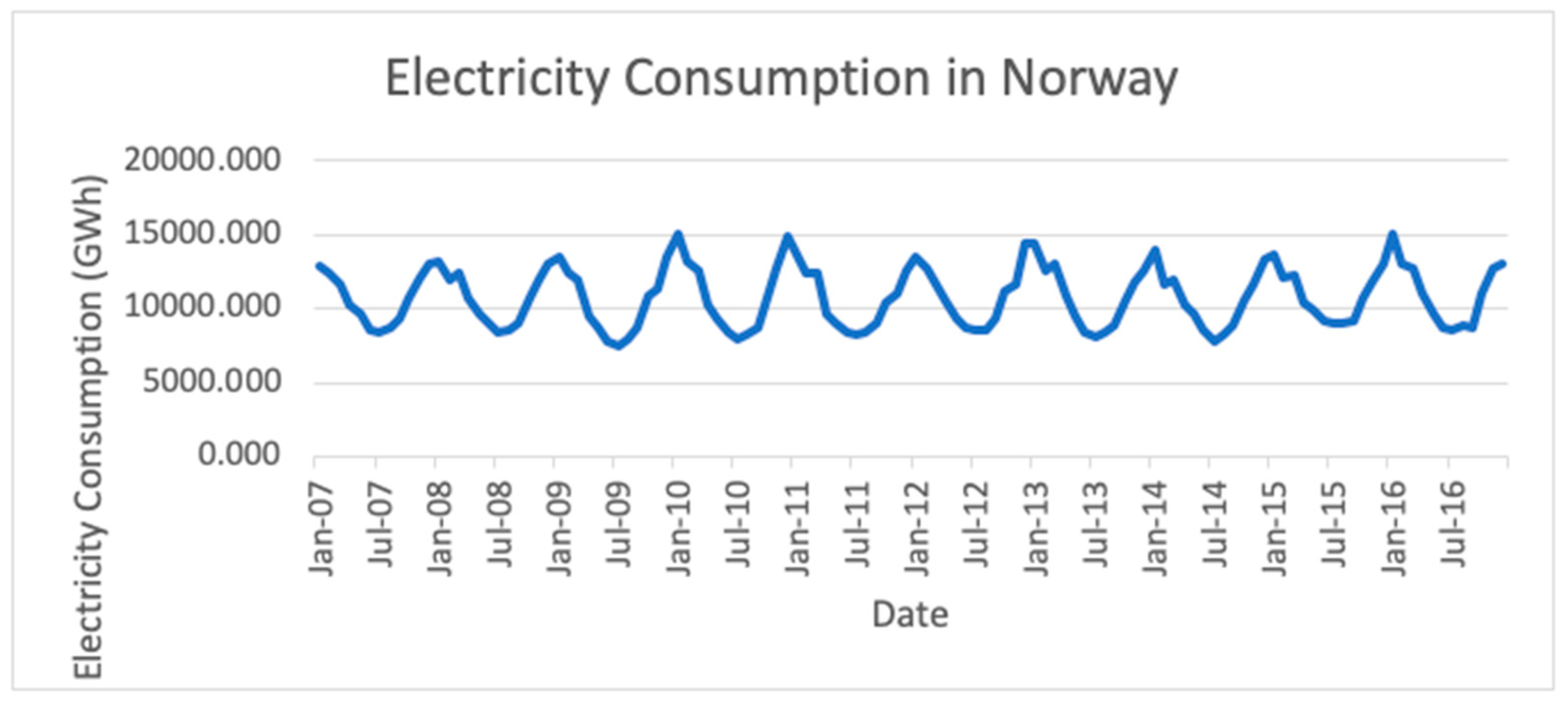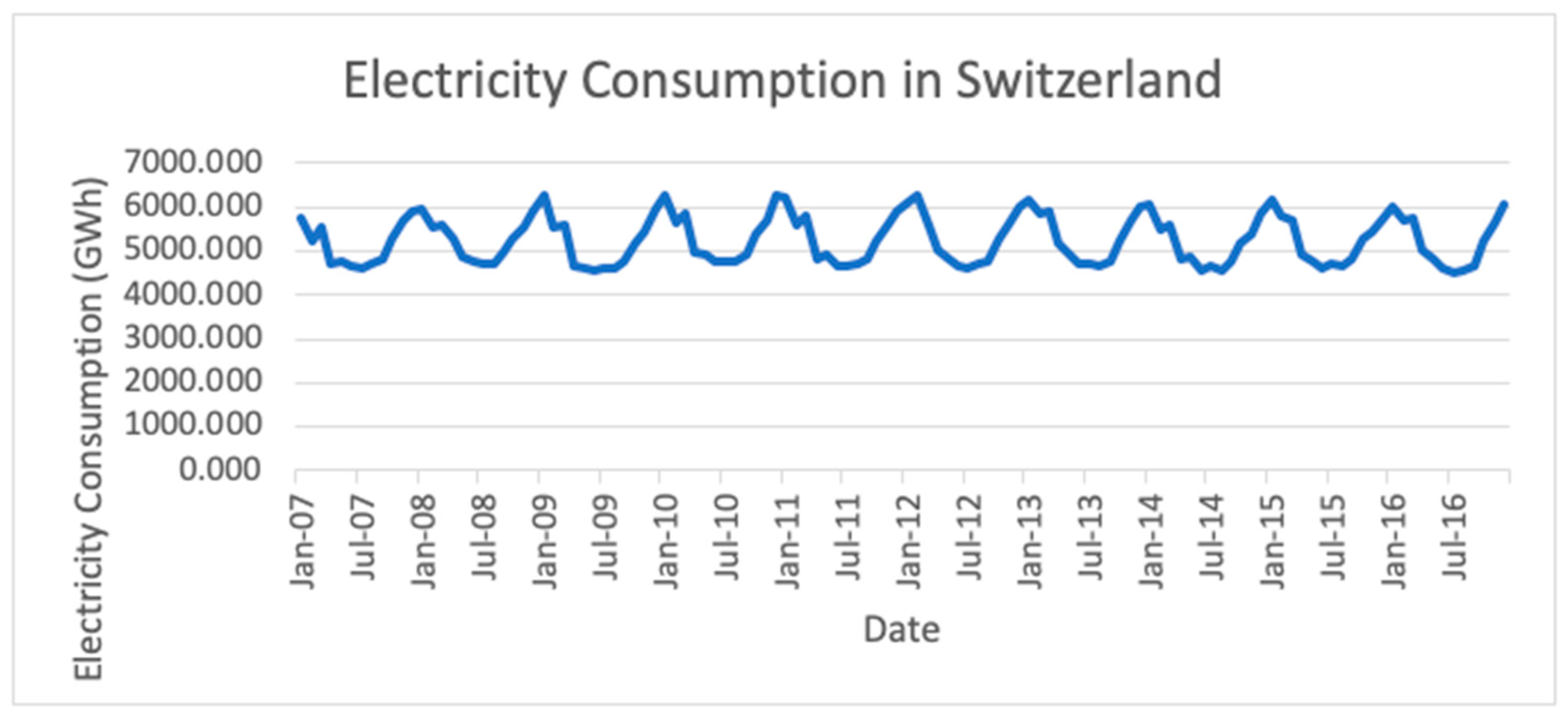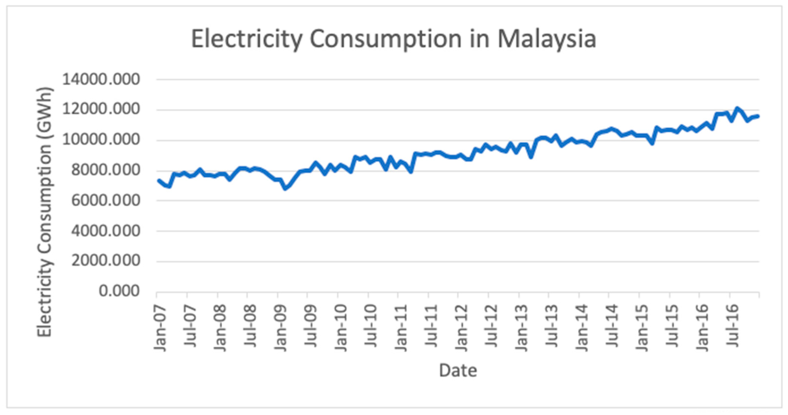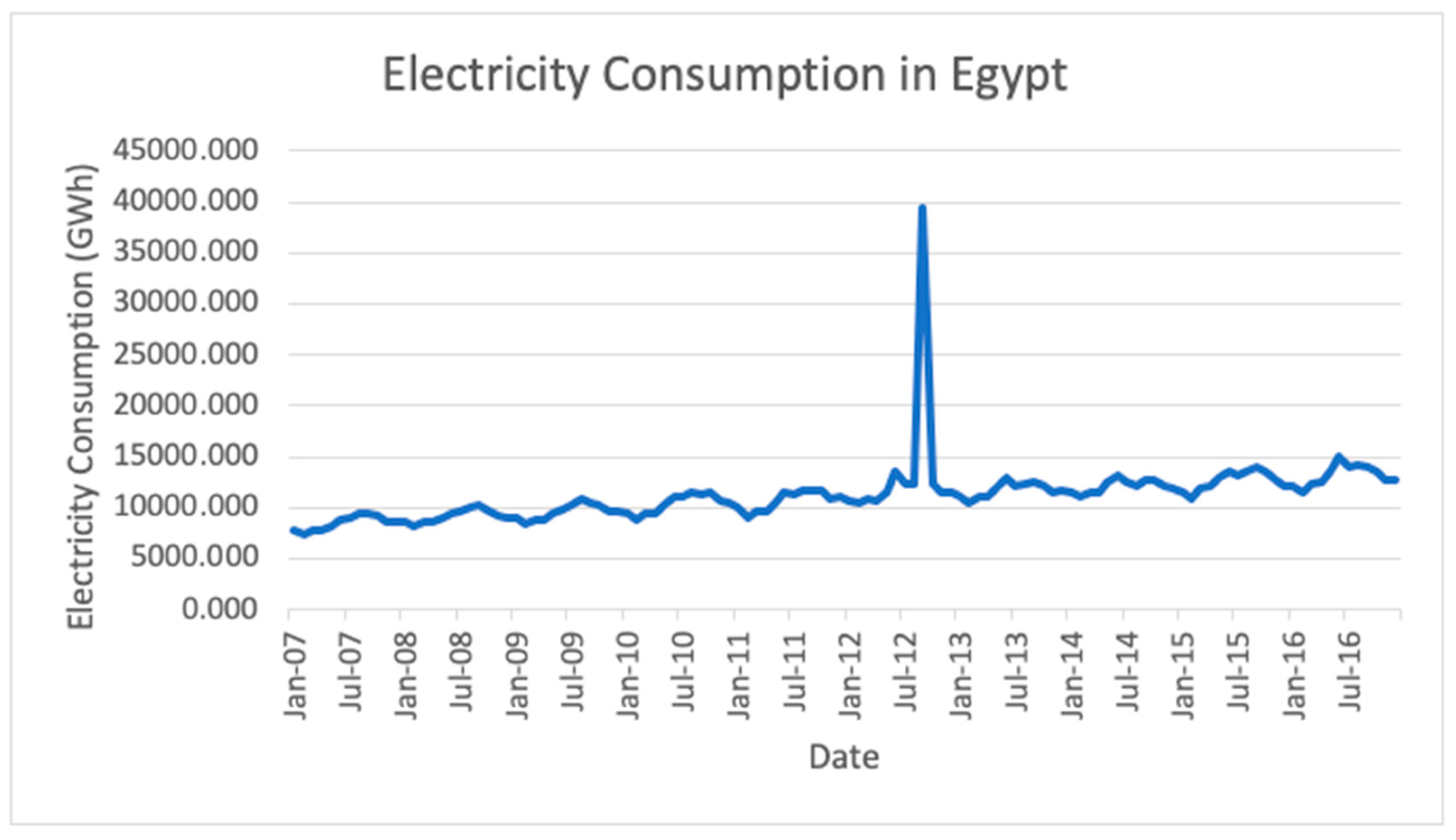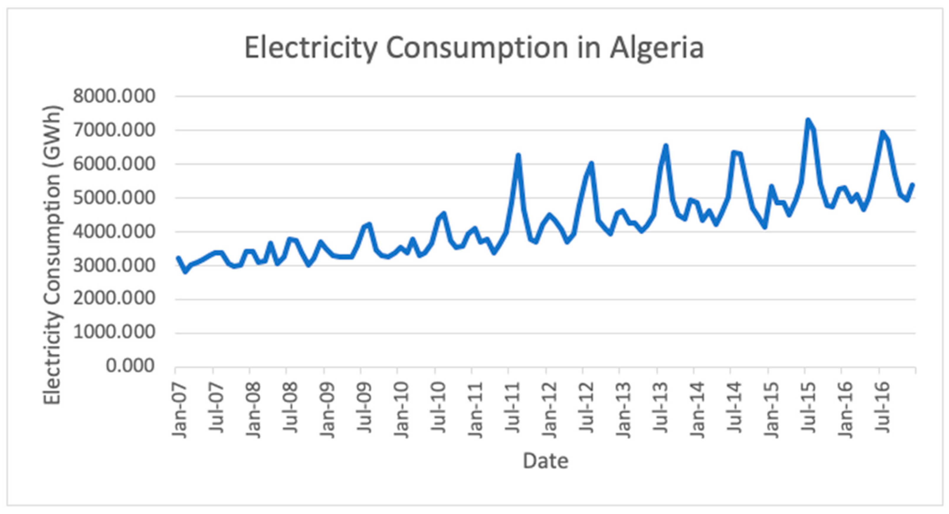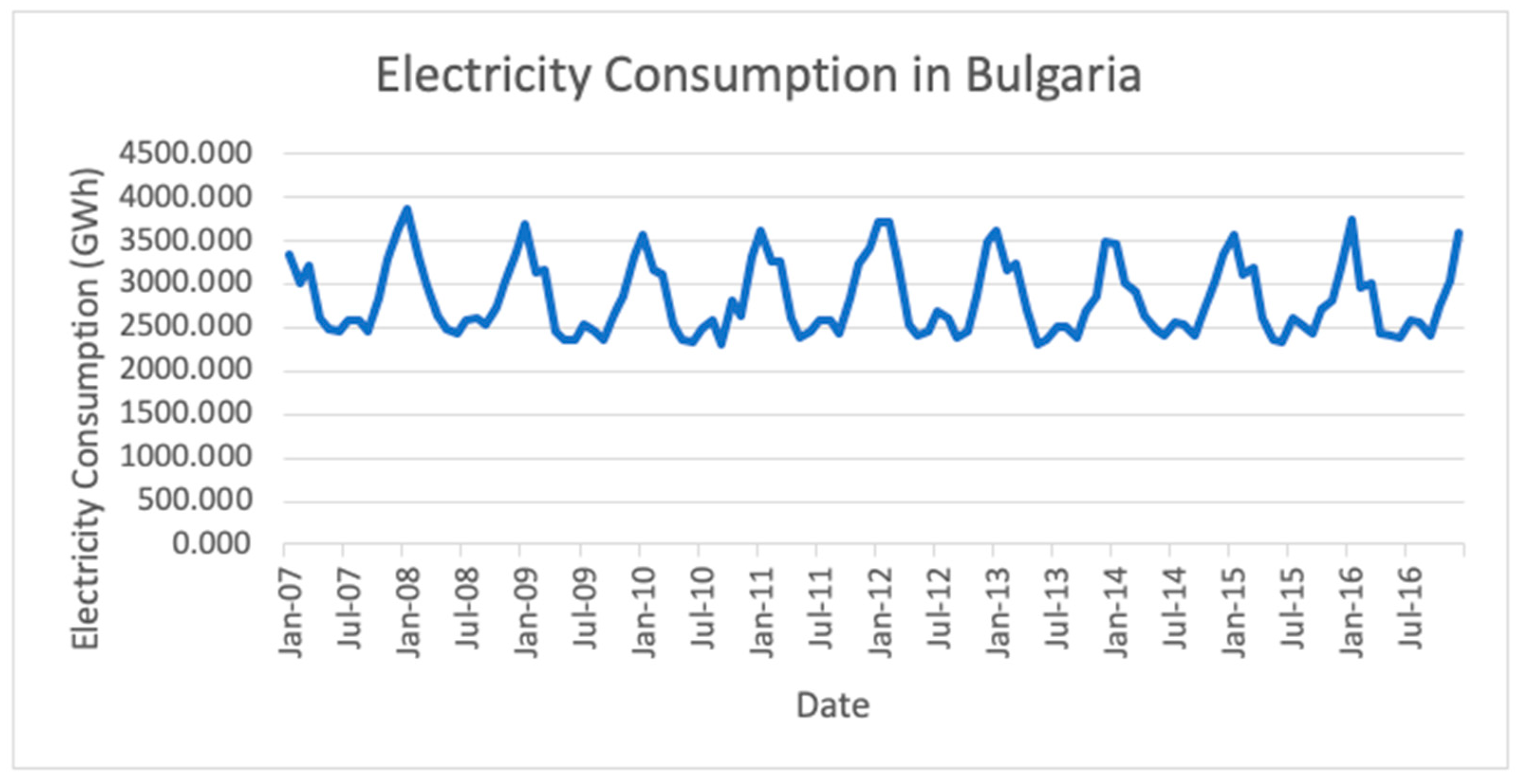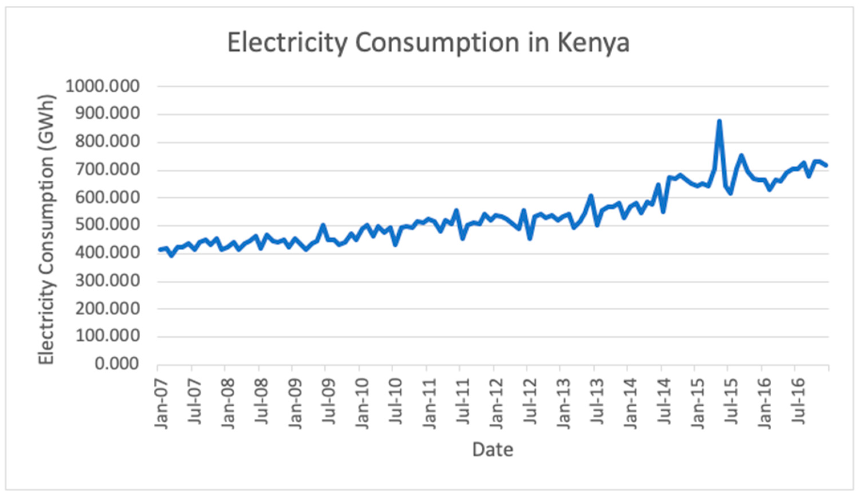Hence, in this study, we investigated the ability of the artificial neural network (ANN) [1], the adaptive neuro-fuzzy inference system (ANFIS) [2], the least squares support vector machines (LSSVMs) [3] and the fuzzy time series model (FTS) [4] to forecast electricity consumption in different countries with different development levels. The forecasting accuracy of these models are also studied and analyzed. The variables considered in this research included the monthly electricity consumption in seven (7) countries: Norway, Switzerland, Malaysia, Egypt, Algeria, Bulgaria and Kenya. The selection of countries was mainly based on their development level, whereby Norway and Switzerland are developed countries; Malaysia, Egypt, Algeria and Bulgaria are developing countries; Kenya is an underdeveloped country.

There have been many research proposals for forecasting electricity consumption. Akdi, Gölveren and Okkaoğlu [5] forecasted daily electricity consumption in Turkey using ARIMA and harmonic regression models. Cevik and Cunkas [6,7], Peng et al. [8] and Tay et al. [9] studied the application of the ANFIS model in forecasting short-term electricity load, while Al-Hamad and Qamber [10] used the ANFIS model to forecast the long-term peak electricity loads of Gulf Cooperation Council member countries, and all of these studies found that the ANFIS model performed better than the other models. Koo and Park [11] used the ANN model to forecast short-term electricity load, while Panklib et al. [12], Ozoh et al. [13] and Azadeh et al. [14] applied the ANN model in forecasting electricity consumption, and all but [11,13] found that the ANN model performed the best compared to the other models. On the other hand, Rahman et al. [15] studied the use of the ANN model for forecasting air quality in Malaysia, while Adebiyi et al. [16] and Laboissiere et al. [17] studied the application of the ANN model for forecasting stock prices, and these studies found that the ANN model produced the most accurate results.

Kaytez et al. [18] applied the LSSVM model for forecasting electricity consumption in Turkey and found that this model performed better than the other models. Pham et al. [19], Ahmadi et al. [20], Kisi and Parmar [21], Deo et al. [22], and Arabloo et al. [23] studied the LSSVM model in environmental forecasting, whereby all but [19,22] found that the LSSVM model performed the best. Efendi et al. [24,25] used the FTS model to forecast the electric load in Taiwan, using Taiwan’s regional electric load from 1981 to 2000, and in the forecasting of the electricity load demand in Malaysia using the daily electricity load data from the National Electricity Board of Malaysia (TNB) from January to August 2006 in [24,25], respectively. Chen [26], Lee et al. [27], and Sun et al. [28] also used the FTS model in forecasting and all of the studies in [24,25,26,27,28] found that the FTS model produced the best results.

There has been also massive research on the use of machine learning models in the area of forecasting, and this has led to an increase in the introduction of hybrid models that combine traditional statistical models with the latest machine learning models [29]. Semero et al. [30] used an integrated GA–PSO–ANFIS method to forecast electricity production, and Göçken et al. [31] introduced a hybrid ANN model that used metaheuristic methods and applied this model to stock price prediction, whereas Shukur and Lee [32] studied daily wind speed forecasting using a hybrid KF–ANN model that was based on the ARIMA model. Chaabane [33] introduced a hybrid ARFIMA and neural network model to forecast electricity prices, while Cerjan et al. [34] and Ardakani and Ardehali [35] studied short-term and long-term electricity forecasting, respectively, using different types of dynamic hybrid models. Khandelwal et al. [36] and Babu and Reddy [37] studied time series forecasting using different types of hybrid ARIMA and ANN models. Kabran and Ünlü [38], on the other hand, used a two-step machine learning approach on the support vector machine (SVM). Yuan et al. [39], Zhu and Chevallier [40], Jung et al. [41] and Li et al. [42] all used various types of hybrid LSSVM models and applied these to problems related to forecasting and prediction. Chen and Chen [43], Dincer and Akkuş [44] and Wang et al. [45] used hybrid FTS models in forecasting stock prices and air pollution, respectively.

Even though studies exist regarding the application of machine learning models to the forecasting of electricity consumption, none have been published to validate and compare several typical forecasting methods within a concrete case study with real data. This paper is structured as follows. In Section 2, we recapitulate the concepts related to the ANN, ANFIS, LSSVM and FTS models. In Section 3, we introduce our proposed methodology on forecasting electricity consumption with the proposed models. In Section 4, the implementation of the methodology is described, and the results are analyzed. Electricity consumption data for the seven studied countries were obtained from ceicdata.com. In Section 5, a summary of our findings is presented. In Section 6, the limitations of this research are presented. Finally, Abbreviations section provides a table of the acronyms that are used throughout the present work and their descriptions.

2. Preliminaries

In this section, we briefly present an introduction to the concepts that are pertinent to the study presented in this paper.

2.1. Artificial Neural Network (ANN)

McCulloch and Pitts [1] introduced this model whereby the neural network structure is based on the neurons in the human nervous system. The dendrites receive information from other neurons, which is processed through synapses and is sent to the axon for output.

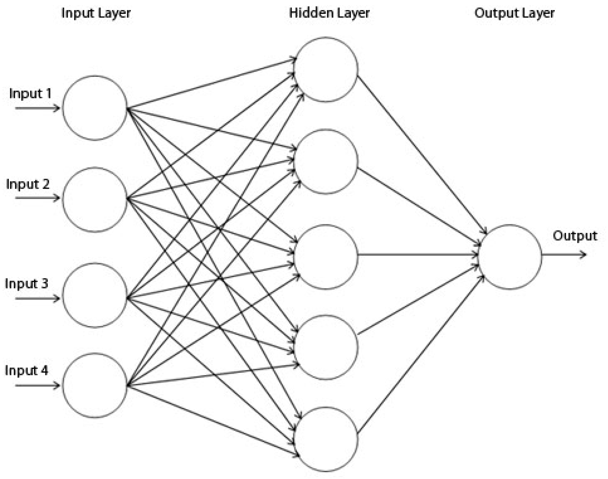
Figure 1 shows an example of the multilayer perceptron (MLP), which is the network structure of the ANN that consists of three layers: the input layer, the hidden layer, and the output layer, all of which are connected through weights. Every neuron in the hidden layer is connected to every neuron in the input layer and the output layer [46]. External information is received from the input layer, and the result is sent out in the output layer. The parameters of the neural network structure are adjusted to identify which structure gives a more accurate result, thus increasing the performance of predicting the testing data [47].

Generally, there is a transfer function that connects the hidden layer to the output, which is given by $g\left(x\right)=1/\left(1+e^{-x}\right)$, where $x$ is the input.

The MLP with only the input layer and the hidden layer can be computed using the equation below:

$$Y_t=W_0+{\displaystyle \sum }_{i=1}^n{W}_i{Y}_i$$

(1)

where $Y_t$ is the output, and $W_i{Y}_i$ denotes the connection weights. The function of the hidden layer is given by:

$$Y_t=W_0+{\displaystyle \sum }_{k=1}^q{W}_k\cdot g\left(W_{0,k}+{\displaystyle \sum }_{j=1}^p{W}_{j,k}\cdot Y_{t-j}\right)+{\epsilon }_t$$

(2)

Referring to Equation (2), the connection weights are denoted as $W_k$ and $W_{j,k}$, while $p$ is the number of input nodes, $q$ is the number of output nodes and ${\epsilon }_t$ is the error term. Thus, Equation (2) maps a nonlinear equation based on the historical observations given by $Y_t=g\left(Y_{t-1},Y_{t-2}, \dots , Y_{t-p}, \omega \right)+{\epsilon }_t$, whereby $g$ is the function formed by the connection weights, and $\omega$ is a vector for all parameters [48].

2.2. Adaptive Neuro-Fuzzy Inference System (ANFIS)

This model was introduced by Jang [2], and it was based on the Takagi–Sugeno inference system. This model was proposed to overcome some of the weaknesses of the ANN model as well as some of the weaknesses of the fuzzy logic system. The ANFIS uses the hybrid learning method to decide the optimal distribution of membership functions in order to obtain the mapping relationship of the input and output data [49].

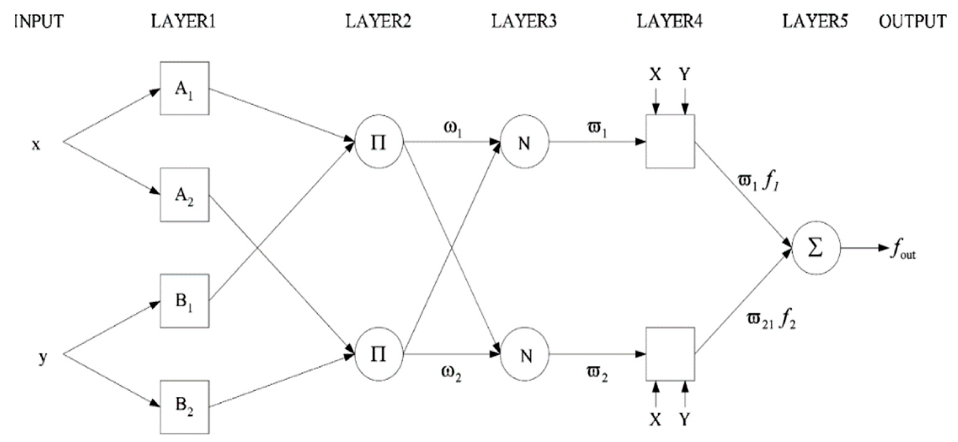
Figure 2 shows the basic ANFIS model consisting of two input data and one output. The rule base of the ANFIS contains the IF–THEN rules of the Sugeno type. The rules are as shown below:

$$\mathrm{Rule}1.\mathrm{If}x\mathrm{is}{A}_1\mathrm{and}y\mathrm{is}{B}_1,\mathrm{then}{f}_1=p_{1}x+q_{1}y+r_1.$$

$$\mathrm{Rule}2.\mathrm{If}x\mathrm{is}{A}_2\mathrm{and}y\mathrm{is}{B}_2,\mathrm{then}{f}_2=p_{2}x+q_{2}y+r_2.$$

where $A_i$ and $B_i$ are known as linguistic variables of the fuzzy sets; $x$ and $y$ are the input data; $p_i$, $q_i$ and $r_i$ are the output parameters. The ANFIS model consists of five layers, and they are explained below. Layer 1 can be known as the fuzzification layer. The nodes are fuzzified in the first layer to provide the output stated as $O_i^1={\mu }_{Ai}\left(x\right), i=1, 2$ and $O_i^1={\mu }_{Bi}\left(y\right), i=3, 4$. Every node in this layer will have a bell function for fuzzification, which is:

$${\mu }_{Ai}\left(x\right)={\mu }_{Bi-2}\left(y\right)=\exp \left[-{\left(\frac{x_i-c_i}{a_i}\right)}^2\right]=\frac{1}{1+{\left\{{\left(\frac{x-c_i}{a_i}\right)}^2\right\}}^{b_i}}$$

(3)

where $x$ is known as the input; $a_i, b_i \mathrm{and} c_i$ are the premise parameters of control; ${\mu }_{Ai}\left(x\right)$ is known as the output.

In Layer 2, every node will be multiplied by input signals to serve as output given as $O_i^2=w_i={\mu }_{Ai}\left(x\right){\mu }_{Bi}\left(y\right), i=1, 2$. The output, $w_i$, is also known as the firing strength of rules.

Layer 3 is the normalization layer, also known as the normalization of the firing strength. The output of the third layer is denoted as $O_i^3=\overline{w_i}=\frac{w_i}{w_1+w_2}$.

Layer 4 is known as the defuzzification stage, where the firing strengths from the third layer are multiplied by the first-order polynomial of the Sugeno model and then normalized. The output is denoted as $O_i^4=\overline{w_i}{f}_i=\overline{w_i}\left(p_{i}x+q_{i}y+r_i\right), i=1, 2$, where $p_i, q_i \mathrm{and} r_i$ are the consequent parameters.

Layer 5 is where all input signals are summed to calculate the overall output of the ANFIS model. The output is denoted as $O_i^5=\frac{{{\displaystyle \sum }}_i{w}_i{f}_i}{{{\displaystyle \sum }}_i{w}_i}$, where $f_i$ is the first-order polynomial based on the first-order Sugeno model.

2.3. Least Squares Support Vector Machines (LSSVMs)

This model was proposed by Suykens and Vandewalles [3] in order to solve quadratic programming (QP) problems faced by the support vector machines (SVMs). Instead of solving QP problems, LSSVMs solve a set of linear equations under the least squares cost function with equality constraints, thus reducing the complexity of computation [51]. Wang and Yu [52] used the LSSVM model to forecast electricity consumption. The modified LSSVM model introduced by Wang and Yu [52] is presented below.

• The modified LSSVM model by Wang and Yu [52] supposing the extracted samples are $D=\left\{\left(x_1,y_1\right),\left(x_2,y_2\right),\dots ,\left(x_N,y_N\right)\right\}$, where $N$ is the number of samples and $x_i$ is the extracted factor vector, $x_i\in R^n$, $y_i\in R$;
• The electricity consumption model, $y=w^T\phi \left(x\right)+b$, is derived from the data $D={\left\{\left(x_i,y_i\right)\right\}}_{i=1}^N$ by minimizing the least squares cost function, $\underset{w,b}{\min }{J}_1\left(w,b\right)=\mu E_w+\zeta E_D$. The regularization and error term are defined as $E_w=\frac{1}{2} w^{T}w$ and $E_D=\frac{1}{2}{{\displaystyle \sum }}_{i=1}^{N}e{i}^2$. Thus, the minimized cost function is $\underset{w,b}{\min }{J}_1\left(w,b\right)=\frac{\mu }{2} w^{T}w+\frac{\zeta }{2} {{\displaystyle \sum }}_{i=1}^{N}e{i}^2$, which is subjected to the constraint $e_i=y_i-\left(w^T\phi \left(x_i\right)+b\right)$, where $i=1,\dots ,N$;
• The Lagrangian function, $L_1\left(w,b,e,\alpha \right)=J_1\left(w,e\right)-{{\displaystyle \sum }}_{i=1}^N{\alpha }_i\left[w^T\phi \left(x_i\right)+b+e_i-y_i\right],$ is constructed by introducing the Lagrange multipliers for equality constraints and taking the conditions for optimality to find the solution for the minimized cost function;
• A linear Karush–Kuhn–Tucker (KKT) system, used to find the load model, is obtained in dual space as $\left[\begin{array}{cc}0& 1_v^T\\ 1_v& \mathsf{\Omega }+{\gamma }^{-1}{I}^N\end{array}\right]\left[\begin{array}{c}b\\ \alpha \end{array}\right]=\left[\begin{array}{c}0\\ Y\end{array}\right]$, where $Y=\left[y_1;\dots ;y_N\right]$, $1_v=\left[1;\dots ;1\right]$, $e=\left[e_1;\dots ;e_N\right]$ and $\alpha =\left[{\alpha }_1;\dots ;{\alpha }_N\right]$;
• Mercer’s condition is applied within $\mathsf{\Omega }$ matrix results in ${\mathsf{\Omega }}_{ij}=\phi {\left(x_i\right)}^T\phi \left(x_j\right)=K\left(x_i,x_j\right)$. The possible kernel functions are linear kernel, $K\left(x_1,x_2\right)=x_1^T{x}_2$ and radial basis function (RBF) kernel, $K\left(x_1,x_2\right)=\exp \left(-\Vert x_1-x_2\Vert {}_2^2/{\sigma }^2\right)$, where Mercer’s condition holds for all possible kernel parameters;
• Then, the electricity consumption regressor is constructed as $y\left(x\right)={\displaystyle \sum }_{i=1}^N{\alpha }_{i}K\left(x,x_i\right)+b$. The mapping relationship of electricity consumption and its extracted influence factors are obtained in this way.

2.4. Fuzzy Time Series (FTS)

In 1965, Zadeh [4] developed the fuzzy set theory in order to solve the vagueness of the data by combining linguistic variables with the analysis process of applying fuzzy logic into time series. Song and Chissom [53] further expanded the study of Zadeh’s fuzzy set theory in forecasting. In 1996, Chen [54] improved the steps involved in the fuzzy time series (FTS) model using simple operations. The main characteristic of Chen’s model is that it uses simple calculations and can provide better forecasting results [55]. The model begins with the process of fuzzification, developing fuzzy logical relationships (FLRs), forming the fuzzy logical group (FLG) and the defuzzification process [25]. The definitions and concepts of FTS forecasting were developed by Song and Chissom [56] as well as by Singh [57].

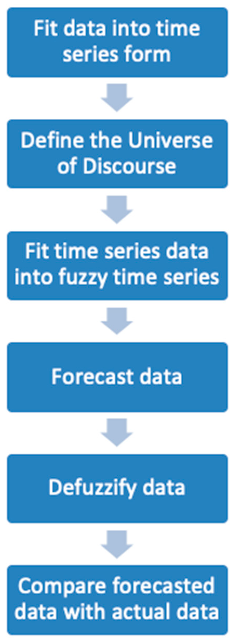
Singh [57] developed a method for time series to solve real-life problems. The steps for FTS forecasting based on historical time series data that were introduced by Singh [57] is presented below (Figure 3):

Step 1: Define the universe of discourse ($U$).

$$U=\left[D_{min}-D_1,D_{max}-D_2\right]$$

(4)

Step 2: Divide the universe of discourse into equal-length intervals, $u_1, u_2, \dots , u_m$, according to the number of linguistic variables, $A_1, A_2, \dots , A_m$. The number of intervals is the same as the number of linguistics variable, which is $m$.

Step 3: Define a fuzzy set for observation according to the intervals in Step 2. The triangular membership rule is applied to each interval in each fuzzy set that is constructed.

Step 4: Fuzzify the historical data.

Step 5: Establish FLRs by the following rule:

Rule: $A_i$ (current state) is a fuzzy production of year $n$, $A_j$ (next state) is a fuzzy production of year $n+1$; then, the FLRs is denoted as $A_i\to A_j$.

Step 6: Determine the forecasting rule.

3. Methodology

In this section, we present the research methods used in this paper. The section also presents a description of the countries studied as well as the utilized data sources, error metrics and forecasting procedures.

3.1. Countries Chosen for the Study

The seven countries studied in this paper were Norway, Switzerland, Malaysia, Egypt, Algeria, Bulgaria and Kenya. The selection of these specific countries was mainly based on their level of development, whereby Norway and Switzerland are developed countries; Malaysia, Egypt, Algeria and Bulgaria are developing countries; Kenya is an underdeveloped country. In this research, the electricity consumption data for the seven countries studied were required in order to train and test the forecasting models. The electricity consumption data were obtained from ceicdata.com; the monthly electricity consumption data for the years 2007 to 2016 were utilized in this study. A data set from the years 2007 to 2015 was used as the training set, while a data set for the year 2016 was used as the testing set.

3.2. Error Metrics

There are many error metrics that can be used to compare the accuracy of the forecasting models such as mean absolute error (MAE), mean absolute deviation (MAD), root mean square error (RMSE), average forecasting error (AFE) and performance parameter (PP). In this paper, the accuracy of the forecasting results was compared using the RMSE, AFE and PP metrics. The reason for using these specific error metrics was because RMSE is the most popular error metric used in regression problems. AFE was used to calculate the mean absolute forecasting error based on the relativeness of the error to the actual value, whereas PP was used to indicate the efficiency of the model. The formulae to calculate these three metrics are as below:

$$\mathrm{RMSE}=\sqrt{\frac{1}{n}{\displaystyle \sum }_i^n{\left(A_i-F_i\right)}^2}$$

(5)

$$\mathrm{AFE}=\frac{1}{n}\left({\displaystyle \sum }_i^n\frac{\left|F_i-A_i\right|}{A_i}\times 100\%\right)$$

(6)

$$\mathrm{PP}=1-\frac{\mathrm{RMSE}}{\sigma }$$

(7)

3.3. Forecasting Procedures

The procedures that were implemented for the forecasting of electricity consumption are briefly expounded upon in this section.

3.3.1. Overview of Forecasting Procedures

The overview of the forecasting process is shown in Figure 4 below.

3.3.2. ANN

The “keras” library in the Spyder IDE (https://keras.io/, accessed on 5 November 2021) was used to model the artificial neural network. The electricity consumption data were normalized using the formula as given below:

$$Normalization of data=\frac{Y_i-mi{n}_y}{ma{x}_y-mi{n}_y}$$

(8)

The normalized data were then imported into the data frame, and the model was trained using 2 hidden layers (6,3). The model was then used to forecast the electricity consumption for 2016.

3.3.3. ANFIS

The computation for the ANFIS was conducted using the Fuzzy Logic toolbox in MATLAB. The training and testing data were imported into workspace. Then, the Neuro-fuzzy Designer window was initiated using anfisedit(). The model was trained and exported to the workspace to generate output values.

3.3.4. LSSVMs

The computation for the LSSVMs was performed using the LSSVMlab toolbox in MATLAB. The training and testing data were imported into the workspace. Then, the model was tuned using the LSSVMlab’s built-in procedure. The model was trained and used to forecast electricity consumption for the year 2016.

3.3.5. FTS

The computation for the FTS was conducted in RStudio using the AnalyseTS package. Figure 3 displays the general procedures for forecasting using the fuzzy time series model. The data set was first imported into RStudio and was fit into a time series. Then, the time series data were fit into Singh’s fuzzy time series model.

4. Performance Evaluation

In this section, a brief overview of the countries studied is discussed. The evaluation of the error metrics computed from the forecasted results and actual results are presented as well.

4.1. Brief Overview of the Countries Studied

In this section, a brief overview of the seven countries that were studied in this paper, namely, Norway, Switzerland, Malaysia, Egypt, Algeria, Bulgaria and Kenya, are presented.

4.1.1. Norway

A plot of Norway’s electricity consumption from 2007 to 2016 is shown in Figure 5. Norway is a highly developed country due to the fact of its high standard of living as well as high human development. Although Norway has a rather low population count, this country has a large energy-intensive manufacturing sector, hence, explaining the high consumption of electricity. Norway experiences winter from December to February every year and also faces polar nights in midwinter, where daylight only lasts for approximately five to six hours. Citizens in Norway may use more electricity during the winter for heating purposes, which explains the higher electricity consumption from December to February. Electricity is widely used to heat up buildings and water in Norway compared to other countries in the world. As Norway experiences summer from June to August, there is a lesser need for citizens to use electricity for heating purposes. Furthermore, hydropower is Norway’s main source of energy, and Norway is able to generate enough energy for their own usage.

4.1.2. Switzerland

A plot of Switzerland’s electricity consumption from 2007 to 2016 is shown in Figure 6. Switzerland is also a highly developed country with low unemployment and a highly skilled labor force. Since Switzerland is already a developed country, the electricity consumption pattern for every year was almost the same. The climate in Switzerland is often moderate, where it does not get too warm during summer or too cold during winter. However, citizens in Switzerland may use more electricity during the winter from December to February for heating purposes. Switzerland’s main source of energy is hydropower, since approximately two-thirds of the country’s land is covered by the Alps, and Switzerland is able to produce enough energy for their own usage.

4.1.3. Malaysia

A plot of Malaysia’s electricity consumption from 2007 to 2016 is shown in Figure 7. Malaysia is a developing country. Even though Malaysia has been undergoing rapid economic growth over the past few years, its standard of living is still not on par with that of developed countries. The major consumers of energy in Malaysia include the manufacturing sector, transportation sector and the domestic sector. As Malaysia has been undergoing periods of economic growth, its electricity consumption has increased for developmental purposes over the years. Malaysia’s climate is hot and humid throughout the whole year; hence, there is no rapid change in electricity consumption throughout the months of every year due to the weather. It also experiences monsoon seasons, which are the northeast monsoon from mid-October to January and the southeast monsoon from June to September. Malaysia’s main source of energy is from the burning of fossil fuels, and Malaysia is able to generate enough energy for their own usage.

4.1.4. Egypt

A plot of Egypt’s electricity consumption from 2007 to 2016 is shown in Figure 8.

Egypt is a developing country, where lately there have been some economic reforms and the building of infrastructure, thereby making Egypt a fast-growing economy. Egypt is one of the countries whereby a large proportion of citizens have access to electricity. The increase in electricity consumption over the years is driven by factors such as population growth, industrial output and economic growth [58]. The climate in Egypt is rather moderate, even though temperatures are lower from December to February. Egypt’s main source of energy is oil, natural gas and hydroelectric power. Egypt is also able to generate enough energy for their own usage with rapid increases each year, especially in September 2012, whereby a number of protests were organized along with political reforms.

4.1.5. Algeria

A plot of Algeria’s electricity consumption from 2007 to 2016 is shown in Figure 9.

Algeria is a slow-developing country with a slightly high unemployment rate. Although Algeria and Malaysia are both developing countries, and the population of Algeria is approximately 10 million more than the population of Malaysia, Algeria has a relatively lower electricity consumption compared to Malaysia. The economy in Algeria is growing too slowly to provide jobs for the increasing population. The temperature in Algeria is moderate with a higher temperature during the month of August, which may explain the increase in electricity consumption for cooling purposes in that month. Algeria’s main source of energy is natural gas. The total energy consumption in Algeria increased by 32% from 2010 to 2014, whereby the increase was mainly in electricity consumption by the residential sector [59].

4.1.6. Bulgaria

A plot of Bulgaria’s electricity consumption from 2007 to 2016 is shown in Figure 10.

Bulgaria is a developing country with a rather high literacy rate and low unemployment rate. Bulgaria has a temperate-continental climate with moderate features with January being the coldest month of the year with an average low temperature of $-3.9 °\mathrm{C}$. This may explain the increase in electricity consumption for heating purposes in the month of January. Approximately 65% of houses in Bulgaria were built in poor condition and with inefficient or non-existent thermal insulation [60]. A study in 2016 stated that 41% of Bulgarians are unable to maintain thermal comfort in their homes due to the fact of rising electricity prices [61]. This has led Bulgarians to use other heat sources, such as coal and wood, which in turn worsens the quality of the air. Bulgaria’s main energy source is coal and nuclear, and they are also able to generate enough energy for their own usage.

4.1.7. Kenya

A plot of Kenya’s electricity consumption from 2007 to 2016 is shown in Figure 11. Kenya is an underdeveloped country where there is limited access to electricity, especially in rural areas. As some of the citizens in Kenya live in poverty, they are also unable to afford electricity. The temperature in Kenya is moderate throughout the whole year. Its electricity consumption is rather stable with slight increases over the years. Approximately 75% of the population in Kenya uses biomass for activities such as cooking and for heating purposes. Electricity only accounts for approximately 9% of the energy source in Kenya [62]. Kenya is able to generate enough energy for its own usage.

4.2. Forecasting the Results for Each of the Forecasting Models

The results of the forecasting of electricity consumption for the year 2016 using the ANN, ANFIS, LSSVM and FTS models for the seven countries that were considered in this study are presented in

Table 1. Forecasting results for the ANN model.

Country	RMSE	AFE	PP
Norway	1041.44	6.692%	0.5324
Switzerland	243.366	4.349%	0.5862
Malaysia	402.031	3.046%	0.0204
Egypt	930.467	5.510%	0.09297
Algeria	644.781	7.815%	0.1147
Bulgaria	310.047	7.986%	0.3264
Kenya	24.9145	2.931%	0.2365

,

Table 2. Forecasting results for the ANFIS model.

Country	RMSE	AFE	PP
Norway	1096.19	7.566%	0.5078
Switzerland	148.11	2.042%	0.7481
Malaysia	439.077	3.327%	−0.0699
Egypt	1503.57	10.125%	−0.4657
Algeria	629.779	8.436%	0.1353
Bulgaria	197.786	4.642%	0.57031
Kenya	59.634	7.103%	−0.8274

,

Table 3. Forecasting results for the LSSVM model.

Country	RMSE	AFE	PP
Norway	2029.66	18.199%	0.08867
Switzerland	659.568	9.929%	−0.12161
Malaysia	1878.88	14.863%	−3.5783
Egypt	1044.99	6.517%	−0.01867
Algeria	1402.33	18.863%	−0.9254
Bulgaria	437.077	14.376%	0.0504
Kenya	45.7663	5.654%	−0.4024

and

Table 4. Forecasting results for the FTS model.

Country	RMSE	AFE	PP
Norway	311.5172	2.279%	0.8601
Switzerland	80.4274	1.419%	0.8632
Malaysia	197.3471	1.357%	0.5191
Egypt	678.3792	4.245%	0.3387
Algeria	179.9432	2.649%	0.7529
Bulgaria	33.7686	1.008%	0.9266
Kenya	14.0048	1.725%	0.5708

.

4.3. Forecasting Results by Country

The forecasting of electricity consumption for different forecasting periods (i.e., short-term and long-term forecasting) for the seven countries were studied for the ANN, ANFIS, LSSVM and FTS models. The short-term and long-term forecasting results for each country are presented in

Table 5. Short-term and long-term forecasting results for Norway.

Error Metrics	Term	Forecasting Period (Months)	Results
			ANN	ANFIS	LSSVM	FTS
RMSE	Short	1	2096.413	1696.852	1922.852	472.412
		2	1460.055	1424.731	1430.165	476.622
		3	1394.546	1169.448	1485.376	434.117
	Long	6	1078.152	863.878	2934.775	360.517
		9	960.801	846.011	2159.390	324.677
		12	1041.438	1096.189	2029.658	311.517
AFE	Short	1	13.902%	11.252%	12.751%	3.133%
		2	9.300%	9.769%	6.908%	3.400%
		3	7.616%	7.059%	7.351%	3.142%
	Long	6	6.699%	5.321%	19.900%	2.782%
		9	6.344%	5.869%	16.278%	2.649%
		12	6.692%	7.566%	18.199%	2.479%

,

Table 6. Short-term and long-term forecasting results for Switzerland.

Error Metrics	Term	Forecasting Period (Months)	Results
			ANN	ANFIS	LSSVM	FTS
RMSE	Short	1	262.208	12.300	68.000	108.271
		2	229.624	63.391	182.180	109.344
		3	247.570	66.025	152.605	93.044
	Long	6	188.855	133.304	726.361	87.479
		9	229.037	111.302	392.951	78.193
		12	243.366	148.110	558.568	80.427
AFE	Short	1	4.345%	0.204%	1.127%	1.794%
		2	3.885%	0.884%	3.062%	1.869%
		3	4.239%	1.001%	2.055%	1.509%
	Long	6	3.258%	2.105%	12.139%	1.526%
		9	4.042%	1.621%	6.323%	1.410%
		12	4.349%	2.042%	9.929%	1.419%

,

Table 7. Short-term and long-term forecasting results for Malaysia.

Error Metrics	Term	Forecasting Period (Months)	Results
			ANN	ANFIS	LSSVM	FTS
RMSE	Short	1	169.870	208.875	1006.775	317.575
		2	216.093	308.832	364.774	217.658
		3	232.151	279.019	777.816	212.657
	Long	6	657.047	419.912	2056.195	266.102
		9	449.889	426.963	1355.522	191.616
		12	402.031	439.077	1878.882	197.347
AFE	Short	1	1.552%	1.909%	9.200%	2.902%
		2	1.896%	2.677%	3.304%	1.967%
		3	1.795%	2.426%	6.914%	1.938%
	Long	6	5.077%	3.120%	16.079%	2.305%
		9	3.431%	3.066%	9.951%	1.290%
		12	3.046%	3.327%	14.863%	1.357%

,

Table 8. Short-term and long-term forecasting results for Egypt.

Error Metrics	Term	Forecasting Period (Months)	Results
			ANN	ANFIS	LSSVM	FTS
RMSE	Short	1	202.510	1944.000	927.000	450.220
		2	491.664	1847.654	595.619	619.783
		3	460.109	1508.609	292.002	537.221
	Long	6	957.278	1281.302	1013.112	772.526
		9	1028.350	1476.916	1054.410	698.380
		12	930.467	1503.568	1044.990	678.379
AFE	Short	1	1.683%	16.153%	7.703%	3.741%
		2	4.122%	15.615%	4.614%	5.118%
		3	3.791%	10.429%	2.412%	4.257%
	Long	6	6.283%	8.839%	6.945%	4.910%
		9	6.429%	9.747%	7.348%	4.292%
		12	5.510%	10.125%	6.517%	4.245%

,

Table 9. Short-term and long-term forecasting results for Algeria.

Error Metrics	Term	Forecasting Period (Months)	Results
			ANN	ANFIS	LSSVM	FTS
RMSE	Short	1	158.350	166.900	369.300	18.768
		2	261.263	300.353	269.208	21.796
		3	160.681	255.136	227.074	128.216
	Long	6	487.918	422.336	376.919	181.178
		9	790.539	698.369	771.629	171.200
		12	644.781	629.779	1402.331	179.943
AFE	Short	1	2.992%	3.154%	6.978%	0.355%
		2	3.563%	5.552%	5.010%	0.426%
		3	2.644%	4.498%	3.469%	1.720%
	Long	6	7.448%	6.913%	6.296%	2.709%
		9	9.704%	9.250%	12.925%	2.519%
		12	7.815%	8.436%	18.863%	2.649%

,

Table 10. Short-term and long-term forecasting results for Bulgaria.

Error Metrics	Term	Forecasting Period (Months)	Results
			ANN	ANFIS	LSSVM	FTS
RMSE	Short	1	413.928	270.500	194.700	13.219
		2	321.005	437.719	384.138	13.079
		3	351.930	359.284	357.663	19.092
	Long	6	329.956	256.268	680.297	28.449
		9	314.810	221.491	387.990	24.638
		12	310.047	197.786	437.077	33.769
AFE	Short	1	11.091%	7.248%	5.217%	0.354%
		2	7.232%	12.985%	11.677%	0.395%
		3	9.756%	9.364%	11.057%	0.567%
	Long	6	9.478%	5.618%	19.979%	0.988%
		9	9.013%	5.172%	9.369%	0.808%
		12	7.986%	4.642%	14.376%	1.008%

and

Table 11. Short-term and long-term forecasting results for Kenya.

Error Metrics	Term	Forecasting Period (Months)	Results
			ANN	ANFIS	LSSVM	FTS
RMSE	Short	1	20.640	12.212	75.044	0.611
		2	27.151	38.796	28.880	17.670
		3	17.957	36.245	30.494	17.482
	Long	6	26.272	43.140	102.902	16.571
		9	28.411	57.988	56.487	15.483
		12	24.914	59.634	45.766	14.005
AFE	Short	1	3.108%	1.839%	11.299%	0.092%
		2	3.486%	5.164%	3.789%	2.028%
		3	2.422%	4.967%	3.755%	2.207%
	Long	6	3.428%	5.658%	15.229%	2.065%
		9	3.727%	6.970%	7.641%	1.983%
		12	2.932%	7.103%	5.654%	1.725%

.

4.4. Analysis and Discussion

The results of the forecasting of electricity consumption for the year 2016 for the seven countries that were studied are tabulated according to the forecasting model and presented in Table 1, Table 2, Table 3 and Table 4, while the results for the short-term and long-term forecasting are tabulated for each country and presented in Table 5, Table 6, Table 7, Table 8, Table 9, Table 10 and Table 11. Table 1 presents the computation results for the ANN model, whereby this model produced the lowest AFE for Kenya, which was 2.931%. The ANN model produced a positive PP for all seven countries, whereby a higher PP value shows greater efficiency of the model. Table 2, on the other hand, presents the computation results for the ANFIS model, whereby this model produced the lowest AFE value of 2.042% and a PP of 0.7481 for Switzerland. The ANFIS model, however, produced a negative PP for Malaysia, Egypt and Kenya, showing that this model was not very efficient in the forecasting of electricity consumption for these countries. Table 3 presents the computation results for the LSSVM model, whereby this model produced the lowest AFE of 5.654% but a negative PP of −0.4024 for Kenya. It also produced a negative PP for Switzerland, Malaysia, Egypt and Algeria, showing that the LSSVM model was not very effective in forecasting electricity consumption for these countries. Table 4 presents the computation results for the FTS model, whereby this model produced the lowest AFE of 1.008% for Bulgaria. The FTS model produced a positive PP for all seven countries studied, which shows that this model was efficient in forecasting electricity consumption.

Table 5 presents the short-term and long-term forecasting results for Norway, whereby the FTS model produced the lowest RMSE for all forecasting periods. Its RMSE was relatively lower than the other models. The FTS model also produced the lowest AFEs for all of the forecasting periods with values of 3.133%, 3.400%, 3.142%, 2.782%, 2.649% and 2.479% for 1, 2, 3, 6, 9 and 12 months, respectively. The FTS model consistently performed the best in forecasting electricity consumption for all forecasting periods in Norway. Table 6 presents the short-term and long-term forecasting results for Switzerland, whereby the ANFIS model produced the lowest RMSEs for short-term forecasting, while the FTS model produced the lowest RMSEs for long-term forecasting. The ANFIS model also produced the lowest AFEs for short-term forecasting at 0.204%, 0.884% and 1.001% for 1, 2 and 3 months, respectively. The FTS model, on the other hand, produced the lowest AFEs for long-term forecasting at 1.526%, 1.410% and 1.419% for 6, 9 and 12 months, respectively. Hence, the ANFIS model was the most accurate for short-term electricity consumption forecasting, while the FTS model was the most accurate for long-term electricity consumption forecasting.

Table 7 presents the short-term and long-term forecasting results for Malaysia, where the ANN model showed the lowest RMSEs for 1 and 2 months of forecasting, while the FTS model showed the lowest RMSEs for 3, 6, 9 and 12 months of forecasting. The ANN model also showed the lowest AFEs for 1, 2 and 3 months at 1.552%, 1.896% and 1.795% respectively, while the FTS model showed the lowest AFEs for 6, 9 and 12 months of forecasting at 2.305%, 1.290% and 1.357%, respectively. Thus, the ANN model was more accurate in short-term forecasting, while the FTS model was more accurate in the long-term forecasting of electricity consumption. Table 8 presents the short-term and long-term forecasting results for Egypt, whereby the ANN model produced the lowest RMSEs for 1 and 2 months of forecasting, while the LSSVM model produced the lowest RMSE for 3 months of forecasting. The FTS model produced the lowest RMSEs for 6, 9 and 12 months. The ANN model produced the lowest AFEs of 1.683% and 4.122% for 1 and 2 months of forecasting, respectively, while the LSSVM produced the lowest AFE of 2.412% for 3 months forecasting. The FTS model on the other hand produced the lowest AFEs for 6, 9 and 12 months of forecasting at 4.910%, 4.292% and 4.245%, respectively. Hence, the ANN model was the most accurate for 1 and 2 months of forecasting, while the LSSVM model was the most accurate for 3 months of forecasting, and the FTS model provided the most accurate results for long-term forecasting.

Table 9 presents the short-term and long-term forecasting results for Algeria, whereby the FTS model produced the lowest RMSE for both short-term and long-term forecasting with RMSEs of 18.768, 21.796, 128.216, 181.178, 171.200 and 179.943 for 1, 2, 3, 6, 9 and 12 months, respectively. The FTS model also produced the lowest AFE compared to the other models. Thus, the FTS model was the most accurate in both short-term and long-term forecasting of electricity consumption in Algeria. Table 10 presents the short-term and long-term forecasting results for Bulgaria, whereby the FTS model produced the lowest RMSEs for 1, 2, 3, 6, 9 and 12 months of forecasting at 13.219, 13.079, 19.092, 28.449, 24.638 and 33.769, respectively. There was also quite a large difference in the RMSEs of the FTS model compared to the other three models. The FTS model also produced the lowest AFEs for both short-term and long-term forecasting. Hence, this shows that the FTS model was the most accurate in both short-term and long-term forecasting of electricity consumption in Bulgaria. Table 11 presents the short-term and long-term forecasting results for Kenya, whereby the FTS model produced the lowest RMSEs for 1, 2, 3, 6, 9 and 12 months of forecasting at 0.611, 17.670, 17.482, 16.571, 15.483 and 14.005, respectively. The FTS model also produced the lowest AFEs for 1, 2, 3, 6, 9 and 12 months of forecasting at 0.092%, 2.028%, 2.207%, 2.065%, 1.983% and 1.725%, respectively. Thus, the FTS model was the most accurate in both long-term and short-term forecasting of electricity consumption in Kenya.

Summary of the main findings: Overall, the different models performed better than others in different forecasting periods and different countries. The ANN model was the most accurate in forecasting short-term electricity consumption in Malaysia as well as 1 and 2 months of forecasting of electricity consumption in Egypt. The ANFIS model was the most accurate in short-term electricity consumption forecasting in Switzerland. The LSSVM model, on the other hand, was the most accurate in 3 months of forecasting of electricity consumption in Egypt. The FTS model was the most accurate in short-term forecasting of electricity consumption in Norway, Algeria, Bulgaria and Kenya. The FTS model was also the most accurate in the long-term forecasting of electricity consumption, which was considered to be 6, 9 and 12 months of forecasting, in all of the seven countries studied in this research. The FTS model was able to perform well and produced low AFEs of less than 6% for all seven countries. This may be due to the ability of the FTS model to perform well with small numbers of data, and the fuzzy component that was present in the FTS model enabled it to capture the uncertainty of the data. The ANN model may not have performed as well as the FTS model because the ANN model requires large numbers of time series data to train the model before it is able to produce accurate results. It can also be seen that the ANFIS model did not perform as well as the FTS model due to the fact that the ANFIS model usually performs better on volatile data. The LSSVM model, on the other hand, was shown to produce the highest AFEs for quite many forecasting periods and different countries. Its lack of accuracy may be due to the fact of its nature as a model that lacks in sparsity. The LSSVM model was also sensitive to the parameters of the kernel function; thus, it was rather difficult to train the model well.

5. Conclusions

The main contributions of this study are summarized below:

• Seven countries were studied in this research, namely, Norway, Switzerland, Malaysia, Egypt, Algeria, Bulgaria and Kenya, and the monthly electricity consumption data for these seven countries from 2007 to 2016 were used as the data sets for this study. The main objective of this study was to determine the best model to forecast electricity consumption with the highest level of accuracy for countries with different characteristics;
• The ANN, ANFIS, LSSVM and FTS models were used to forecast the electricity consumption for the year 2016 for the seven selected countries. These four models showed differing performances in different forecasting periods and in the forecasting of electricity consumption for the different countries. The ANN model was found to be the most accurate model in forecasting short-term electricity consumption for Malaysia as well as for 1 and 2 months of forecasting electricity consumption in Egypt. The ANFIS model was found to be the most accurate model in short-term electricity consumption forecasting in Switzerland. The LSSVM model, on the other hand, was found to be the most accurate model for 3 months of forecasting electricity consumption in Egypt. The FTS model was found to be the most accurate model for short-term forecasting of electricity consumption in Norway, Algeria, Bulgaria and Kenya. The FTS model was also found to be the most accurate model for the long-term forecasting of electricity consumption for the periods of 6, 9 and 12 months for all of the seven countries that were studied in this research;
• In terms of long-term forecasting, the FTS model was found to be the most accurate model and produced the lowest AFEs for all seven countries that were studied. This may be due to the ability of the FTS model to perform well with small numbers of data, and the fuzzy component that is present in the FTS model enabled it to capture the uncertainty of the data;
• From the graphs of the electricity consumption patterns for the seven countries that were studied in this paper, it can be seen that Norway, Switzerland and Bulgaria had a rather similar electricity consumption pattern, while Algeria’s electricity consumption pattern had a higher peak during August, instead of a peak between the months of December and February. Malaysia, Egypt and Kenya, on the other hand, had a more stable electricity consumption pattern, although Egypt’s electricity consumption had an obvious outlier. Although the seven countries that were studied had different electricity consumption patterns, the FTS model was found to perform the best and consistently produced the lowest AFE values compared to the other models;
• The application of predictive models in the forecasting of electricity consumption and production is continuously gaining ground in the area of power generation due to the fact of their improved accuracy and increased ability to handle complex relationships and to uncover hidden patterns in big data. Among the most commonly applied supervised learning approaches for electricity consumption and production forecasting are ML models, such as ANNs and SVMs, and metaheuristic methods, such as fuzzy logic-based approaches that include the ANFIS and FTS models. This can be seen from the various studies that were expounded upon in Section 1 of this paper. The absence of a clearly defined answer to every problem and the fact that different results may be produced, even for the same problem, but under different circumstances, makes comparative studies involving different ML models highly relevant and an important component of the body of knowledge in that area of research. Furthermore, due to the complex nature of electricity consumption, which involves many different factors, it is a challenging task to compare the performance of different models/methods that are used in forecasting electricity consumption. Hence, our study, which compared the performances of the ANN, ANFIS, FTS and LSSVM models, is in fact adequate, as it studied the performance of several of the most commonly applied supervised learning approaches in the context of electricity consumption. Our study contributes to the continuous efforts of the research community to assess the performances of various ML models to develop accurate data-driven forecasting models for the forecasting of electricity consumption.

6. Limitations and Future Research

The limitations of this study are as given below:

(i)

Monthly electricity consumption data for 10 years for seven countries was used in this research. It would have been better if daily or hourly electricity consumption data were used, as many machine learning methods work best with large amounts of data, and the use of larger amounts of data for training of the models would also produce better forecasts. However, it is rather difficult to obtain daily or even hourly electricity consumption data of countries. Better forecasts would be more useful, as it would enable electricity management companies, city councils and governments to better estimate the amount of electricity needed to be supplied to each region in a country.

Some suggestions for future research are as given below:

(ii)

It is recommended for future studies in this area to use a larger size of sample data, as increasing the numbers of data would help improve the accuracy of the forecasts that are produced;

(iii)

It is recommended to consider a larger number of countries in future studies in this area. The difficulty in obtaining electricity consumption data for many countries led to only seven countries being considered in this study. Using longer periods of data for a larger number of countries would enable future research in this area to study the electricity consumption patterns of different countries to be able to draw more conclusive and convincing conclusions.