A Fractional-Order Compartmental Model of Vaccination for COVID-19 with the Fear Factor

Abstract

During the past several years, the deadly COVID-19 pandemic has dramatically affected the world; the death toll exceeds 4.8 million across the world according to current statistics. Mathematical modeling is one of the critical tools being used to fight against this deadly infectious disease. It has been observed that the transmission of COVID-19 follows a fading memory process. We have used the fractional order differential operator to identify this kind of disease transmission, considering both fear effects and vaccination in our proposed mathematical model. Our COVID-19 disease model was analyzed by considering the Caputo fractional operator. A brief description of this operator and a mathematical analysis of the proposed model involving this operator are presented. In addition, a numerical simulation of the proposed model is presented along with the resulting analytical findings. We show that fear effects play a pivotal role in reducing infections in the population as well as in encouraging the vaccination campaign. Furthermore, decreasing the fractional-order parameter $\alpha$ value minimizes the number of infected individuals. The analysis presented here reveals that the system switches its stability for the critical value of the basic reproduction number $R_0=1$.

1. Introduction

Coronavirus belongs to an outsized family of viruses causing illness in both people and animals, including camels, cats, and bats. COVID-19 results in a respiratory disease caused by a SARS-CoV-2, which belongs to the family of severe acute respiratory syndrome coronavirus 2 (SARS-CoV-2). Mostly, SARS-CoV-2-infected people experience mild to moderate symptoms and recover without any treatment. However, many others require medical attention due to comorbidity factors or weak immunity.

In humans, COVID-19 transmission occurs directly via respiratory droplets from coughing or sneezing or indirectly through contaminated objects or surfaces. These particles range from larger respiratory droplets to smaller aerosols [1]. The virus spreads more easily indoors and in crowded settings. People who are in close contact with a suspected/confirmed COVID-19 patient thus often suffer from this virus in turn. In human civilization, COVID-19 is the fastest-growing infectious disease among all other such diseases in the world. By the first week of October 2021, more than 238 million cases have been reported [2] worldwide [3] and among these, more than 4.8 million were fatal cases. The World Health Organization (WHO) declared COVID-19 a worldwide pandemic on 11 March 2020 [4]. The COVID-19 pandemic has had a significant impact on pediatric surgery residency programs.

The recovery rate is the main hope for this pandemic. Every country has implemented a Standard Operating Procedure (SOP) for controlling and reducing the outbreak. Various strategies, such as social distancing, wearing masks, regular hand washing, a ban on air traffic, and bans on social gatherings in different areas have all been considered. Various countries and local administrations have enforced lockdowns in the most affected areas to control social gatherings and halt the chain of transmission of this infectious disease. Scientific/academic institutions and manufacturers have worked on developing COVID-19 vaccines, and they have succeeded in achieving their goals to an extent.

In December 2020, a Pfizer/BioNTech vaccine was listed with the WHO. AstraZeneca’s collaboration with Oxford University invented the SII/Covishield and AstraZeneca/AZD1222 vaccines, manufactured by the Serum Institute of India and SK Bio, respectively. This vaccine received EUL on 16 February. Johnson & Johnson developed the Janssen/Ad26.COV 2.S vaccine, which was listed for EUL on 12 March 2021. In April 2021, the Moderna COVID-19 vaccine (mRNA 1273) was listed for EUL; the Sinopharm COVID-19 vaccine was listed for EUL on 7 May 2021. The Sinovac-CoronaVac was listed for EUL on 1 June 2021 [4]. It has been reported that 44.9% of the world’s population has received at least one dose of the COVID-19, vaccine and about 26.02 million are now being vaccinated each day. However, the vaccine’s efficacy is questionable for new variants of the virus. Thus, media awareness around maintaining SOP remains needed in order to control and break the transmission chain of the pandemic.

Statistical data analysis leads to the development of real-world mathematical models. These models are analyzed to understand changes in the dynamical behavior of viruses. Infections such as HIV, HCV, and COVID-19 have been modeled by mathematical formulas and analyzed in an attempt to determine their dynamics. During the present pandemic period, several mathematical models have been proposed to study COVID-19 on both the micro-level and macro-level [5,6,7,8,9,10,11,12,13,14,15]. The mathematical study of such models includes stability theory, local and global dynamics, optimal control theory, and numerical simulation. The infection dynamics of COVID-19 were studied by Atangana [10] using fractional order differential equations. Tang et al. [11] calculated the basic reproduction number for COVID-19 infection. Sarkar and Khajanchi [12] formulated a mathematical model to study SARS CoV-2 infection dynamics and validated their model with real-world data from India. Liu et al. [16] considered reported and unreported cases to study disease transmission using data from China. Samui et al. [17] discussed a compartmental mathematical model based on reported and unreported symptomatic individuals in India. Mondal et al. [8] studied the effects of non-pharmaceutical and pharmaceutical interventions intended to control COVID-19.

In unpredictable situations, classical derivatives become inadequate due to the uncertainty factor [18,19,20,21,22,23,24]. In the case of COVID-19 there are number of ambiguities, including the source of the outbreak, changes in the incubation period, the asymptomatic stage of certain infected individuals, etc. Thus, studying diseases through classical differential equations is quite challenging. To cope with this situation, fractional-order models play a pivotal role in fitting data and studying the complex dynamics involved [25]. Several mathematicians have studied the disease models using fractional calculus as well [2,26,27,28,29,30,31,32].

In the present work, we propose a model addressing two new issues: (a) the effects of fear on transmission rates of infection; and (b) the reinfection of vaccinated individuals. In our proposed model, we consider the Caputo fractional derivative operator [2] for the COVID-19 disease model. The subsequent content of this article is organized as follows:

The fundamental concepts of fractional calculus are recalled in Section 2. The basic mathematical results of our proposed model of COVID-19 are presented in Section 3. A mathematical model with a Caputo fractional derivative operator setting is analyzed in Section 4, and the existence of solutions for the proposed model is investigated. In Section 5, we discuss the numerical simulation of the model. Finally, the results of the fractional-order model are summarized in the concluding section.

2. Fundamental Concepts of Fractional Derivatives in the Caputo Sense

Here, we recall the fundamental concepts regarding the Caputo derivative.

The left-sided Caputo fractional derivative [33] is defined as

$$\begin{array}{c}\hfill {}_a^C{D}_t^{\alpha }g\left(t\right)=\frac{1}{\Gamma (n-\alpha )}{\int }_a^t\frac{g^{\left(n\right)}\left(s\right)}{{(t-s)}^{\alpha -n+1}}ds\end{array}$$

(1)

and the right-sided Caputo fractional derivative [33] is defined as

$$\begin{array}{c}\hfill {}_t^C{D}_b^{\alpha }g\left(t\right)=\frac{{(-1)}^n}{\Gamma (n-\alpha )}{\int }_t^b\frac{g^{\left(n\right)}\left(s\right)}{{(t-s)}^{\alpha -n+1}}ds.\end{array}$$

(2)

Here $\alpha$ with $n-1<\alpha <n$ is the order of derivative and the gamma function is symbolized as $\Gamma$, where n is an integer.

The left-sided Riemann–Liouville fractional derivative [33] is defined as

$$\begin{array}{c}\hfill {}_a{D}_t^{\alpha }g\left(t\right)=\frac{1}{\Gamma (n-\alpha )}\frac{d^n}{d{t}^n}{\int }_a^t\frac{g\left(s\right)}{{(t-s)}^{\alpha -n+1}}ds\end{array}$$

(3)

and the right-sided Riemann–Liouville fractional derivative [33] is defined as

$$\begin{array}{c}\hfill {}_t{D}_b^{\alpha }g\left(t\right)=\frac{{(-1)}^n}{\Gamma (n-\alpha )}\frac{d^n}{d{t}^n}{\int }_t^b\frac{g\left(s\right)}{{(t-s)}^{\alpha -n+1}}ds.\end{array}$$

(4)

The order of derivative is denoted as $\alpha$ with $n-1<\alpha <n$ and the gamma function is symbolized as $\Gamma$ with n as an integer; $a>0$, $b>0$ are constants. Throughout this article, $D_t^{\alpha }$ and $D_{t_f}^{\alpha }$ are used to indicate the Left-Caputo and Right-Caputo derivative, respectively.

3. Model with Vaccination

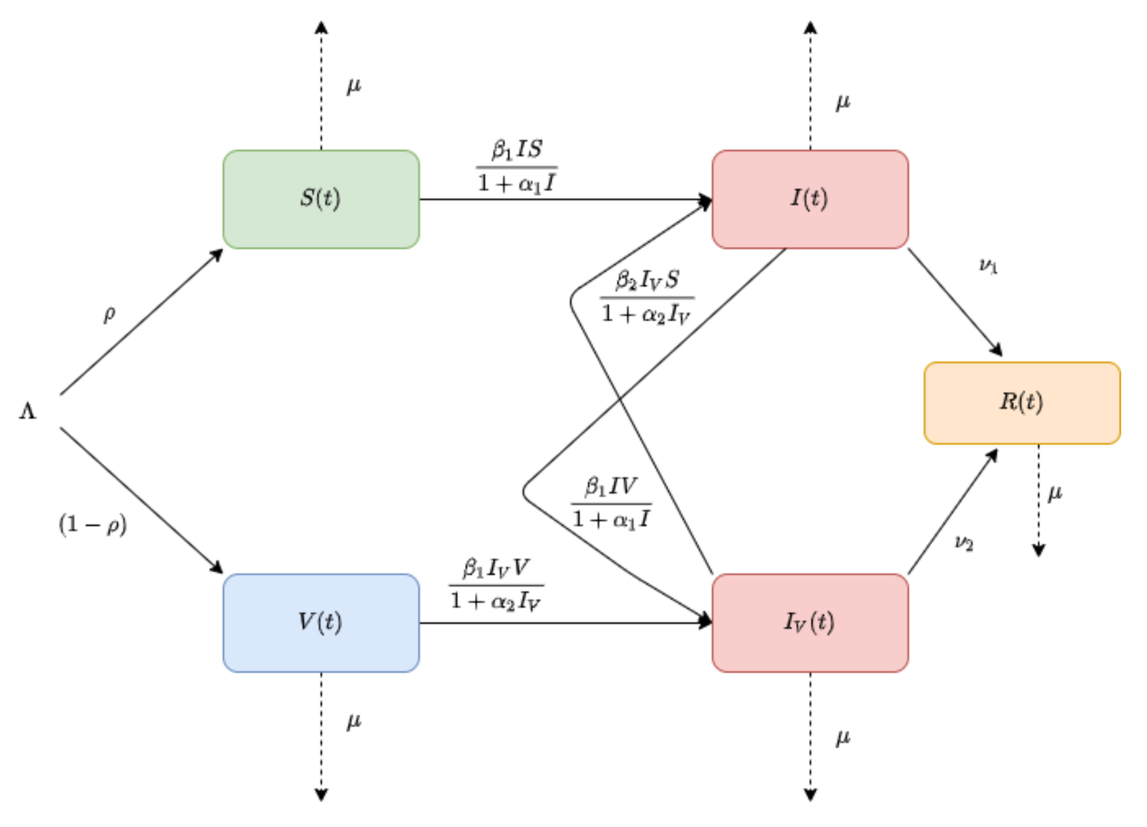
In this article, we propose a compartmental model of the SIR (Susceptible–Infected–Recovered) type, including a vaccine strategy for COVID-19 with the assumption that a fixed proportion of individuals entering the model are temporarily immune to infection (see Figure 1).

We consider that there is no disease-specific death and the death rate for all classes is $\mu$. The introduction and removal rates are assumed to be constant.

Let $S,$I, and R represent the susceptible, infected, and recovered populations, respectively. We denote by V the vaccinated population, while $I_V$ represents the infected population after vaccination.

The birth rate is $\Lambda$, with a vaccinated proportion $\rho$. The transmissible function is $\beta (I,I_V)$, where $\beta (I,I_V)=\frac{{\beta }_{1}I}{1+{\alpha }_{1}I}+\frac{{\beta }_2{I}_V}{1+{\alpha }_2{I}_V}$.

Here, ${\alpha }_1$ and ${\alpha }_2$ are the corresponding fear factors before and after vaccination. Here, ${\nu }_1$ is the recovery rate before vaccination and ${\nu }_2$ is the recovery rate after vaccination in infected individuals.

Thus, the basic model with vaccination takes the following form:

$$\begin{array}{ccc}\hfill \frac{dS}{dt}& =& \rho \Lambda -\frac{{\beta }_{1}SI}{1+{\alpha }_{1}I}-\frac{{\beta }_{2}S{I}_V}{1+{\alpha }_2{I}_V}-\mu S,\hfill \\ \hfill \frac{dI}{dt}& =& \frac{{\beta }_{1}SI}{1+{\alpha }_{1}I}+\frac{{\beta }_{2}S{I}_V}{1+{\alpha }_2{I}_V}-({\nu }_1+\mu )I,\hfill \\ \hfill \frac{dV}{dt}& =& (1-\rho )\Lambda -\frac{{\beta }_{1}VI}{1+{\alpha }_{1}I}-\frac{{\beta }_{2}V{I}_V}{1+{\alpha }_2{I}_V}-\mu V,\hfill \\ \hfill \frac{d{I}_V}{dt}& =& \frac{{\beta }_{1}VI}{1+{\alpha }_{1}I}+\frac{{\beta }_{2}V{I}_V}{1+{\alpha }_2{I}_V}-({\nu }_2+\mu )I_V,\hfill \\ \hfill \frac{dR}{dt}& =& {\nu }_{1}I+{\nu }_2{I}_V-\mu R,\hfill \end{array}$$

(5)

with the biologically realistic non-negative initial conditions

$$\begin{array}{c}\hfill S\left(t_0\right)=S_0,I\left(t_0\right)=I_0,V\left(t_0\right)=V_0,I_V\left(t_0\right)=I_{V_0},R\left(t_0\right)=R_0.\end{array}$$

(6)

Numerous studies have been focused on fractional order systems [2,29] in the study of disease dynamics. On the basis of Section 2, we applied a general fractional derivative to extend the above model. Thus, the modified model with fractional order is obtained by

$$\begin{array}{ccc}\hfill D_t^{\alpha }S& =& \rho \Lambda -\frac{{\beta }_{1}SI}{1+{\alpha }_{1}I}-\frac{{\beta }_{2}S{I}_V}{1+{\alpha }_2{I}_V}-\mu S,\hfill \\ \hfill D_t^{\alpha }I& =& \frac{{\beta }_{1}SI}{1+{\alpha }_{1}I}+\frac{{\beta }_{2}S{I}_V}{1+{\alpha }_2{I}_V}-({\nu }_1+\mu )I,\hfill \\ \hfill D_t^{\alpha }V& =& (1-\rho )\Lambda -\frac{{\beta }_{1}VI}{1+{\alpha }_{1}I}-\frac{{\beta }_{2}V{I}_V}{1+{\alpha }_2{I}_V}-\mu V,\hfill \\ \hfill D_t^{\alpha }{I}_V& =& \frac{{\beta }_{1}VI}{1+{\alpha }_{1}I}+\frac{{\beta }_{2}V{I}_V}{1+{\alpha }_2{I}_V}-({\nu }_2+\mu )I_V,\hfill \\ \hfill D_t^{\alpha }R& =& {\nu }_{1}I+{\nu }_2{I}_V-\mu R,\hfill \end{array}$$

(7)

where the initial conditions are $S\left(t_0\right)=S_0,I\left(t_0\right)=I_0,V\left(t_0\right)=V_0,I_V\left(t_0\right)=I_{V_0},R\left(t_0\right)=R_0$. The Left-Caputo fractional derivative is indicated by $D_t^{\alpha }$.

All state variables are considered to be non-negative, while the state variable are positive for the time period $t\ge 0$.

Remark 1.

In this study, our main focus is to verify the effectiveness of vaccination strategies for COVID-19 infection. It is true that there are several existing models which include the exposed and asymptomatic classes and which have been used to describe the short-term dynamics. Here, however, as we are interested in vaccination-induced changes in the system, we deliberately omitted the variables for the exposed and asymptomatic classes by assuming that at steady state these two classes are proportional to the infected population. This can be shown using steady state approximation theory as well (for example, see [34,35]), that is, the two classes can be approximated by the infected class.

4. Mathematical Analysis

To analyze its existence and uniqueness, system (7) can be rewritten in the following form:

$$\begin{array}{c}\hfill D_t^{\alpha }x\left(t\right)=f(t,x\left(t\right)),0<\alpha \le 1,\end{array}$$

(8)

where $f(t,x)={(f_1,f_2,f_3,f_4,f_5)}^T$, and the initial conditions are

$$x\left(0\right)={(S\left(0\right),I\left(0\right),V\left(0\right),I_V\left(0\right),R\left(0\right))}^T,$$

where the derivative is assumed in Left-Caputo. Additionally, $f_1,f_2,f_3,f_4,f_5$ are the right hand side of system (7); for example, $f_1=\rho \Lambda -\frac{{\beta }_{1}SI}{1+{\alpha }_{1}I}-\frac{{\beta }_{2}S{I}_V}{1+{\alpha }_2{I}_V}-\mu S,$ etc. The function $f(t,x):\mathbb{R}\times {\mathbb{R}}^d⟶{\mathbb{R}}^d$ defines a vector field with dimension $d\ge 1$.

4.1. Local and Global Existence and Uniqueness of Solution

We consider the function $X\left(t\right):R_0{,}_{+}⟶R_0{,}_{+}$, defined by

$$\begin{array}{ccc}\hfill X\left(t\right)& =& f_1\left(t\right)+f_2\left(t\right)+f_3\left(t\right)+f_4\left(t\right)+f_5\left(t\right).\hfill \end{array}$$

(9)

Note that the function $X\left(t\right)$ is well-defined and differentiable on the interval (0, $t_f$). After simple calculation, we obtain

$$\begin{array}{ccc}\hfill X\left(t\right)& =& \Lambda -\mu [S\left(t\right)+I\left(t\right)+V\left(t\right)+I_V+R\left(t\right)].\hfill \end{array}$$

(10)

With the help of the theorem stated below (from [36]), we can establish the existence of the solution of the fractional-ordered system (7).

Theorem 1.

Let $\mathbb{J}=[t_0-a,t_0+a]$, $\mathbb{B}=\{x\in {\mathbb{R}}^d|\Vert x-x_0\Vert \le b\}$ and $\mathbb{D}=\{(t,x)\in \mathbb{R}\times {\mathbb{R}}^d|t\in J,x\in \mathbb{B}\}$ where the function $f:\mathbb{D}⟶{\mathbb{R}}^d$ satisfies the conditions stated below:

• (i) $f(t,x)$ is Lebesgue measurable on $\mathbb{J}$ with respect to t ,
• (ii) $f(t,x)$ is continuous on $\mathbb{B}$ with respect to x ,
• (iii) There exists a real-valued function $m\left(t\right)\in L^5\left(J\right)$ such that $f(t,x)\le m\left(t\right)$ for almost every $t\in J$ and all $x\in B$.

Then, for $\alpha >\frac{1}{2}$ there exists at least one solution of the system

$$D_t^{\alpha }x\left(t\right)=f(t,x\left(t\right)),0<\alpha \le 1,$$

on the interval $[t_0-h,t_0+h]$ for some $h>0$.

Now, system (7) with conditions (8) can be considered as an initial value problem (IVP). It is obvious that the right-hand sides of system (8), i.e., $f_1,f_2,f_3,f_4,f_5$ are continuous on $\mathbb{B}$, measurable on $\mathbb{J}$, and bounded for all $t\in [t_0-h,t_0+h]$. Again, if we assume $f(x,t)={(f_1,f_2,f_3,f_4,f_5)}^T$, then from (8) it can be said that $f(x,t)$ satisfies all the conditions of Theorem 1, with $m\left(t\right)=\Lambda -\mu x\left(t\right),x\left(t\right)=S\left(t\right)+I\left(t\right)+V\left(t\right)+I_V+R\left(t\right)$.

Hence, there exists a solution of system (7) in $(0,t_f)$ with initial condition (8). Using the following theorem [36], the uniqueness of the solution can be studied.

Theorem 2.

Let the conditions (i)–(iii) of Theorem 1 hold. Suppose that a real-valued function $\zeta \left(t\right)\in L^5\left(\mathbb{J}\right)$ exists, and

$$\begin{array}{c}\hfill \Vert f(t,x)-f(t,y)\Vert \le \zeta \left(t\right)\Vert x-y\Vert \end{array}$$

(11)

for almost every $t\in \mathbb{J}$ and all $x,y\in \mathbb{B}$; then, the system

$$D_t^{\alpha }x\left(t\right)=f(t,x\left(t\right)),0<\alpha \le 1,$$

possesses a unique solution on the interval $[t_0-h,t_0+h]$ for some $h>0$.

For the our system (7), using (10) we can write the following:

$$\begin{array}{c}\hfill \Vert f(t,x)-f(t,y)\Vert \le \zeta \left(t\right)\Vert x-y\Vert ,\end{array}$$

(12)

where $\zeta \left(t\right)\le \frac{\Lambda }{\mu }$. Thus, the conditions of Theorem 2 are true for the fractional ordered system (7). Hence, system (7) possesses a unique solution.

With the help of the following Theorem (Theorem 3.1 from [36]), the global existence of the solution for system (7) can be verified.

Theorem 3.

Let the vector field $F(t,x)$ satisfy the first two conditions of the above Theorem 2 and Theorem 2 in the global space and $\Vert f(t,x)\Vert \le w+l\Vert x\Vert$ for almost every $t\in \mathbb{R}$ and all $x\in {\mathbb{R}}^d$, with $w,l>0$. Then, a function $x\left(t\right)$ can be obtained on $(-\infty ,+\infty )$ by solving the IVP (7) with initial condition (8).

Using (10) and the property of norm, we can write

$$\begin{array}{ccc}\hfill \Vert f(x,t)\Vert & \le & \Lambda +\mu \Vert x\Vert .\hfill \end{array}$$

(13)

Thus, system (7) satisfies all the conditions of a global existence theorem with $w=\Lambda$ and $l=\mu$. Thus, a solution of system (7) exists globally.

4.2. Basic Reproductive Number $R_0$

The basic reproduction number for system (7) can be calculated with the help of the next-generation matrix method [37,38]. Here, the infected compartments of system (7) are $I,I_V,R$. At the infection-free steady state $\widehat{E}$ and rate of appearance of new infections, $\mathcal{M}$ and $\mathcal{N}$, the rates of transition of infection are defined as:

$$\begin{array}{ccc}\hfill \mathcal{M}& =& \left(\begin{array}{c}\frac{{\beta }_{1}SI}{1+{\alpha }_{1}I}+\frac{{\beta }_{2}S{I}_V}{1+{\alpha }_2{I}_V}\\ \frac{{\beta }_{2}VI}{1+{\alpha }_{1}I}+\frac{{\beta }_{2}V{I}_V}{1+{\alpha }_2{I}_V}\\ 0\end{array}\right),\mathcal{N}=\left(\begin{array}{c}({\nu }_1+\mu )I\\ ({\nu }_2+\mu )I_V\\ -({\nu }_{1}I+{\nu }_2{I}_V-\mu R)\end{array}\right).\hfill \end{array}$$

Next, we assume the matrix $\mathcal{M}$ as the entry-wise non-negative new infection matrix. Let the non-singular Metzler matrix for the transitions of COVID-19 infection between the infectious compartments be defined as $\mathcal{N}$ where $M,N$ are as follows:

$$\begin{array}{ccc}\hfill M& =& \left(\begin{array}{ccc}{\beta }_1\widehat{S}& {\beta }_2\widehat{S}& 0\\ {\beta }_1\widehat{V}& {\beta }_2\widehat{V}& 0\\ 0& 0& 0\end{array}\right),N=\left(\begin{array}{ccc}({\nu }_1+\mu )& 0& 0\\ 0& ({\nu }_2+\mu )& 0\\ 0& 0& \mu \end{array}\right).\hfill \end{array}$$

It can be seen that $N^{-1}$ is similarly a non-negative matrix, and consequently $M{N}^{-1}$ is a non-negative next-generation matrix presenting the estimated number of new infections, which is provided by

$$\begin{array}{c}\hfill M{N}^{-1}=\left(\begin{array}{ccc}\frac{{\beta }_1\widehat{S}}{\mu (\mu +{\nu }_2)}& \frac{{\beta }_2\widehat{S}}{\mu (\mu +{\nu }_1)}& 0\\ \frac{{\beta }_1\widehat{V}}{\mu (\mu +{\nu }_2)}& \frac{{\beta }_2\widehat{S}}{\mu (\mu +{\nu }_1)}& 0\\ 0& 0& 0\end{array}\right).\end{array}$$

With the help of the spectral radius of the next-generation matrix, we obtain the basic reproduction number of system (7) as

$$\begin{array}{ccc}\hfill R_0& =& \frac{{\beta }_1\widehat{S}}{\mu (\mu +{\nu }_2)}+\frac{{\beta }_2\widehat{V}}{\mu (\mu +{\nu }_1)}\hfill \\ & =& \frac{{\beta }_1\rho \Lambda }{{\mu }^2(\mu +{\nu }_2)}+\frac{{\beta }_2(1-\rho )\Lambda }{{\mu }^2(\mu +{\nu }_1)}\hfill \\ & =& R_0^1+R_0^2.\hfill \end{array}$$

(14)

Remark 2.

Note that $R_0$ has two parts, the first is $R_0^1$ and the second $R_0^2$. The first term refers to human-to-human transmission (susceptible-to-infected and infected-to-susceptible). The second, $R_0^2$, refers to human-to-human disease transmission after vaccination. The system changes from disease-free to an endemic state when $R_0$ crosses the value 1. The entire infection risk for COVID-19 is considered through this transmission mode during vaccination.

5. Existence of Equilibria and Stability

The recovered population, $R\left(t\right)$, has no impact on other populations. Thus, it is sufficient to study the dynamics of the following system:

$$\begin{array}{ccc}\hfill D_t^{\alpha }S& =& \rho \Lambda -\frac{{\beta }_{1}SI}{1+{\alpha }_{1}I}-\frac{{\beta }_{2}S{I}_V}{1+{\alpha }_2{I}_V}-\mu S,\hfill \\ \hfill D_t^{\alpha }I& =& \frac{{\beta }_{1}SI}{1+{\alpha }_{1}I}+\frac{{\beta }_{2}S{I}_V}{1+{\alpha }_2{I}_V}-({\nu }_1+\mu )I,\hfill \\ \hfill D_t^{\alpha }V& =& (1-\rho )\Lambda -\frac{{\beta }_{1}VI}{1+{\alpha }_{1}I}-\frac{{\beta }_{2}V{I}_V}{1+{\alpha }_2{I}_V}-\mu V,\hfill \\ \hfill D_t^{\alpha }{I}_V& =& \frac{{\beta }_{1}VI}{1+{\alpha }_{1}I}+\frac{{\beta }_{2}V{I}_V}{1+{\alpha }_2{I}_V}-({\nu }_2+\mu )I_V,\hfill \\ \hfill D_t^{\alpha }R& =& {\nu }_{1}I+{\nu }_2{I}_V-\mu R,\hfill \end{array}$$

(15)

with the initial conditions: $S\left(0\right)=S_0,I\left(0\right)=I_0,V\left(0\right)=V_0,I_V\left(0\right)=I_{V_0}.$ In model (15), there always exists a disease-free equilibrium $\widehat{E}=(\widehat{S},\widehat{I},\widehat{V},\widehat{I_V},\widehat{R})=(\frac{\rho \Lambda }{\mu },0,\frac{(1-\rho )\Lambda }{\mu },0,0)$.

When COVID-19 infection continues in the system, there is a unique positive endemic steady state, $E^{*}=(S^{*},I^{*},V^{*},I_V^{*})$, which can be obtained by equating the right-hand side of the model (15) to zero and is provided by

$$\begin{array}{c}\hfill \left\{\begin{array}{c}\rho \Lambda -\frac{{\beta }_{1}SI}{1+{\alpha }_{1}I}-\frac{{\beta }_{2}S{I}_V}{1+{\alpha }_2{I}_V}-\mu S=0,\\ \frac{{\beta }_{1}SI}{1+{\alpha }_{1}I}+\frac{{\beta }_{2}S{I}_V}{1+{\alpha }_2{I}_V}-({\nu }_1+\mu )I=0\\ (1-\rho )\Lambda -\frac{{\beta }_{1}VI}{1+{\alpha }_{1}I}-\frac{{\beta }_{2}V{I}_V}{1+{\alpha }_2{I}_V}-\mu V=0,\\ \frac{{\beta }_{1}VI}{1+{\alpha }_{1}I}+\frac{{\beta }_{2}V{I}_V}{1+{\alpha }_2{I}_V}-({\nu }_2+\mu )I_V=0.\end{array}\right\}\end{array}$$

(16)

Solving (16), we obtain

$$\begin{array}{c}\hfill \left\{\begin{array}{cc}{V}^{*}=\frac{(1-\rho )\Lambda -({\nu }_2+\mu )I_V^{*}}{\mu }=\varphi (I^{*},I_V^{*}),& \\ S^{*}=\frac{\rho \Lambda -({\nu }_1+\mu )I^{*}}{\mu }={\psi }_1(I^{*},I_V^{*}),& \\ S^{*}=\rho \Lambda {\left[\frac{{\beta }_1{I}^{*}}{1+{\alpha }_1{I}^{*}}+\frac{{\beta }_2{I}_V^{*}}{1+{\alpha }_2{I}_V^{*}}+\mu \right]}^{-1}={\psi }_2(I^{*},I_V^{*}),& \\ S^{*}=({\nu }_1+\mu )I^{*}{\left[\frac{{\beta }_1{I}^{*}}{1+{\alpha }_1{I}^{*}}+\frac{{\beta }_2{I}_V^{*}}{1+{\alpha }_2{I}_V^{*}}\right]}^{-1}={\psi }_3(I^{*},I_V^{*}).\end{array}\right\}\end{array}$$

(17)

Considering the three curves ${\psi }_i(I,I_V),i=1,2,3$, for $I,I_V\ge 0$, the endemic equilibrium can be determined in ${\mathbb{R}}_{+}^3$ by the interaction of these three curves as

$$\begin{array}{ccc}\hfill {\psi }_1(0,0)& =& \frac{\rho \Lambda }{\mu }=\widehat{S},\hfill \\ \hfill {\psi }_1(I_1,0)& =& 0\Rightarrow I_1=\frac{\rho \Lambda }{\mu +{\nu }_1},\hfill \\ \hfill {\psi }_2(0,0)& =& \frac{\rho \Lambda }{\mu }.\hfill \end{array}$$

(18)

Observe that ${\psi }_3(I_1,I_V)$ is an increasing function. Now, we deduce that:

(A)

When $R_0>1$, $S={\psi }_1(I,I_V)$, then $S={\psi }_2(I,I_V),S={\psi }_3(I,I_V)$ are in the interior of ${\mathbb{R}}_{+}^3$ and have a unique interaction ${\psi }_2(0,0)\ge {\psi }_3(0,0)$ and ${\psi }_2(I,I_V)\le {\psi }_3(I,I_V)$. Moreover, at the given interaction point system (17) attains a unique endemic equilibrium, $E^{*}$.

(B)

There is no interaction point of these three curves in the interior of ${\mathbb{R}}_{+}^3$ whenever $R_0\le 1$, as the model has a disease-free equilibrium when $R_0\le 1$.

Thus, it can be concluded that model (15) has a disease-free equilibrium $\widehat{E}$ if $R_0\le 1$. On the contrary, if $R_0>1$, then model (15) attains another equilibrium other than disease-free equilibrium, that is, endemic equilibrium.

Finally, we obtain the following result for the existence of endemic equilibrium, $E^{*}$.

Theorem 4.

System (15) represents the SARS-CoV-2 viral infection dynamics; there exists a threshold parameter around the infection-free equilibrium point, specifically the basic reproduction number $R_0$ where $R_0>1$ results in the existence of a unique positive endemic steady state $E^{*}$ for system (15).

Stability of Equilibria

The Jacobian matrix at any equilibrium point $E(S,I,V,I_V)$ is provided by

$$\begin{array}{ccc}\hfill J_{{|}_E}& =& \left(\begin{array}{cccc}-(a_{11}+\mu )& -a_{12}& 0& -a_{13}\\ a_{11}& a_{12}-(\mu +{\nu }_1)& 0& a_{13}\\ 0& -a_{32}& -(a_{11}+\mu )& -a_{34}\\ 0& a_{32}& a_{11}& a_{34}-(\mu +{\nu }_2)\\ 0& {\nu }_1& 0& {\nu }_2\end{array}\right),\hfill \end{array}$$

(19)

where

$$\begin{array}{cc}\hfill a_{11}=& \frac{{\beta }_{1}I}{1+{\alpha }_{1}I}+\frac{{\beta }_2{I}_V}{1+{\alpha }_2{I}_V},a_{12}=\frac{{\beta }_{1}S}{{(1+{\alpha }_{1}I)}^2},\hfill \\ \hfill a_{13}=& \frac{{\beta }_{2}S}{{(1+{\alpha }_2{I}_V)}^2},a_{32}=\frac{{\beta }_{1}V}{{(1+{\alpha }_{1}I)}^2},a_{34}=\frac{{\beta }_{2}V}{{(1+{\alpha }_2{I}_V)}^2}.\hfill \end{array}$$

(20)

The characteristic equation is obtained from the equation

$$|J-x{I}_{4\times 4}|=0,$$

and is provided by

$$\begin{array}{ccc}\hfill x^4+{\lambda }_1{x}^3+{\lambda }_2{x}^2+{\lambda }_{3}x+{\lambda }_4& =& 0,\hfill \end{array}$$

(21)

where

$$\begin{array}{cc}\hfill {\lambda }_1=& 2a_{11}-a_{12}-a_{34}+2\mu +{\nu }_1+{\nu }_2,\hfill \\ \hfill {\lambda }_2=& a_{11}{a}_{34}+(a_{11}+a_{12})\mu +{\nu }_1(a_{11}+\mu )+{\mu }^2\hfill \\ \hfill & +(a_{11}-a_{12}+2\mu +{\nu }_1)(a_{11}-a_{34}+2\mu +{\nu }_2)-a_{13}{a}_{32},\hfill \\ \hfill {\lambda }_3=& (a_{11}-a_{34}+2\mu +{\nu }_2)a_{11}{a}_{34}\hfill \\ \hfill & +\{(a_{11}+a_{12})\mu +{\nu }_1(a_{11}+\mu )+{\mu }^2\}(a_{11}-a_{34}+2\mu +{\nu }_2)+2\mu a_{13}{a}_{32},\hfill \\ \hfill {\lambda }_4=& a_{13}{a}_{32}(a_{11}-a_{34}+2\mu +{\nu }_2)+{\mu }^2{a}_{13}{a}_{32}.\hfill \end{array}$$

(22)

Considering the discriminant of a characteristic polynomial denoted by $D\left(\epsilon \right)$. If $\epsilon \left(x\right)=x^4+{\lambda }_1{x}^3+{\lambda }_2{x}^2+{\lambda }_{3}x+{\lambda }_4=0$, then

$$D\left(\epsilon \right)=\left|\begin{array}{ccccccc}1& {\lambda }_1& {\lambda }_2& {\lambda }_3& {\lambda }_4& 0& 0\\ & & & & & & \\ 0& 1& {\lambda }_1& {\lambda }_2& {\lambda }_3& {\lambda }_4& 0\\ & & & & & & \\ 0& 0& 1& {\lambda }_1& {\lambda }_2& {\lambda }_3& {\lambda }_4\\ & & & & & & \\ 4& 3{\lambda }_1& 2{\lambda }_2& {\lambda }_3& 0& 0& 0\\ & & & & & & \\ 0& 4& 3{\lambda }_1& 2{\lambda }_2& {\lambda }_3& 0& 0\\ & & & & & & \\ 0& 0& 4& 3{\lambda }_1& 2{\lambda }_2& {\lambda }_3& 0\\ & & & & & & \\ 0& 0& 0& 4& 3{\lambda }_1& 2{\lambda }_2& {\lambda }_3\end{array}\right|.$$

From [39,40], we obtain the following proposition.

Proposition 1.

Suppose equilibria E of system (15) exist in $R_{+}^4$. Now:

(i)

Define $b_1$, $b_2$, and $b_3$ as the Routh–Hurwitz discriminants where, $b_1={\lambda }_1$, $b_2={\lambda }_1{\lambda }_2-{\lambda }_3$, and

$$b_3=\left|\begin{array}{ccc}{\lambda }_1& 1& 0\\ & & \\ {\lambda }_3& {\lambda }_2& {\lambda }_1\\ & & \\ 0& {\lambda }_4& {\lambda }_3\\ & & \end{array}\right|.$$

When $\alpha =1$ and if the below conditions

$$\begin{array}{c}\hfill b_1>0,b_2>0,b_3=0and{\lambda }_4>0\end{array}$$

(23)

are satisfied, then the equilibrium point E is locally asymptotically stable.

(ii)

If $D\left(\epsilon \right)>0$, ${\lambda }_1>0$, ${\lambda }_2<0$ and $\alpha >\frac{2}{3}$, then then the equilibrium point E is unstable.

(iii)

If the inequalities $D\left(\epsilon \right)<0$, ${\lambda }_1>0$, ${\lambda }_2>0$, ${\lambda }_3>0$, ${\lambda }_4>0$ and $\alpha <\frac{1}{3}$ hold, then E is locally asymptotically stable, and unstable if $D\left(\epsilon \right)<0$, ${\lambda }_1<0$, ${\lambda }_2>0$, ${\lambda }_3<0$ and ${\lambda }_4>0$.

(iv)

If the conditions $D\left(\epsilon \right)<0$, ${\lambda }_1>0$, ${\lambda }_2>0$, ${\lambda }_3>0$, ${\lambda }_4>0$ and ${\lambda }_2=\frac{{\lambda }_1{\lambda }_4}{{\lambda }_3}+\frac{{\lambda }_3}{{\lambda }_1}$ hold, then for $\alpha \in (0,1)$ E is locally asymptotically stable.

(v)

A necessary condition for the steady state E to be locally asymptotically stable is ${\lambda }_4>0$.

The stability of the disease-free $\widehat{E}$ and interior equilibrium point $E^{*}$ in $R_{+}^4$ can be determined using Equation (21) and Proposition 1. The coefficients at the endemic equilibrium point can be determined and verified, and their stabilities can be studied using MATLAB.

Remark 3.

The criterion provided in (23) (Routh–Hurwitz criterion) is only the condition for E to be locally asymptotic for $\alpha =1$, not for all $\alpha \in [0,1)$.

6. Numerical Simulations

In this subsection, our main aim is to find the effect of vaccination against COVID-19 infection in the Caputo form provided by model (7) through numerical analysis. The numerical method for the system of fractional order differential, (7), was developed from the existing Matlab code as presented in [41].

For the numerical simulation, the numerical solution of the COVID-19 vaccinated model Equation (7) is found by considering different values of the fractional order parameter $\alpha$.

The birth rate is $\Lambda$, with a vaccinated proportion $\rho$. The transmissible function is $\beta (I,I_V)$, where $\beta (I,I_V)=\frac{{\beta }_{1}I}{1+{\alpha }_{1}I}+\frac{{\beta }_2{I}_V}{1+{\alpha }_2{I}_V}$. Here, ${\alpha }_1$ and ${\alpha }_2$ denote the corresponding fear factors before and after vaccination, ${\nu }_1$ is the recovery rate before vaccination, and ${\nu }_2$ is the recovery rate after vaccination in infected individuals.

In this section, we aim to perform the numerical simulation of system (5) and (7) using MATLAB and the baseline parameter values listed in

Table 1. Description and values of the parameters.

Dependent Variables	Description
S	Susceptible Population
I	Infected Population
V	vaccinated population
$I_V$	Infected population
	after vaccination
R	Recovered Population
Parameter	Description	Values	Reference
$\Lambda$	Birth rate (per week)	270	[42]
$\rho$	Probability of vaccination	0–1	-
${\beta }_1$	Infection rate without vaccination	0.0075	[2,11]
${\beta }_2$	Infection rate after vaccination	0.0007	[11]
${\alpha }_1$	Fear effect before vaccination	0.02–2	Assumed
${\alpha }_2$	Fear effect after vaccination	0.02–2	Assumed
$\mu$	natural death rate	0.3	[2]
${\nu }_1$	Recovery rate before vaccination	0.01	[43]
${\nu }_2$	Recovery rate before vaccination	0.3	[43]

. In the presence of vaccination and fear factors, the system is practically changeable, and selection of parameters is an exciting task.

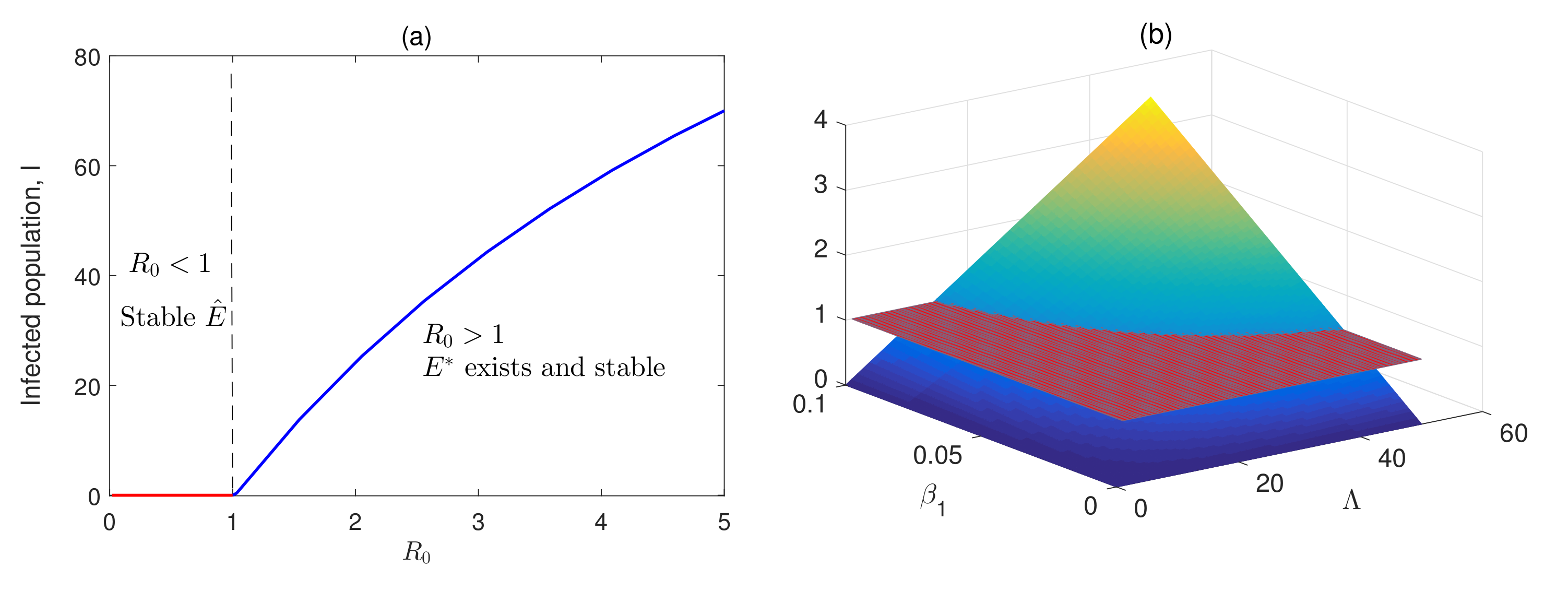
Figure 2 (left panel) represents the dynamic behavior of the system through numerical simulation. In this figure, we have varied the infection rates ${\beta }_1$ and ${\beta }_2$ to find the existence of the equilibrium of the system for different values of $R_0$. It can be observed that for a lower infection rate, the system attains a disease-free state $\widehat{E}$ that corresponds to $R_0>1$ and system $\widehat{E}$ becomes unstable, and hence $E^{*}$ exists. Figure 2 (right panel) represents the color bar scheme. Here, we determine the surface, $R_0$, the surface $R_0=1$ by changing ${\beta }_1$ and $\Lambda$, the disease transmission rate, and the production rate, respectively . When $\beta$ decreases, $R_0$ will decline and range below 1, and the system moves to its infection-free state. Additionally, $R_0$ can be controlled by reducing $\Lambda$. Thus, both vaccination and the fear effect play a pivotal role in controlling disease progression.

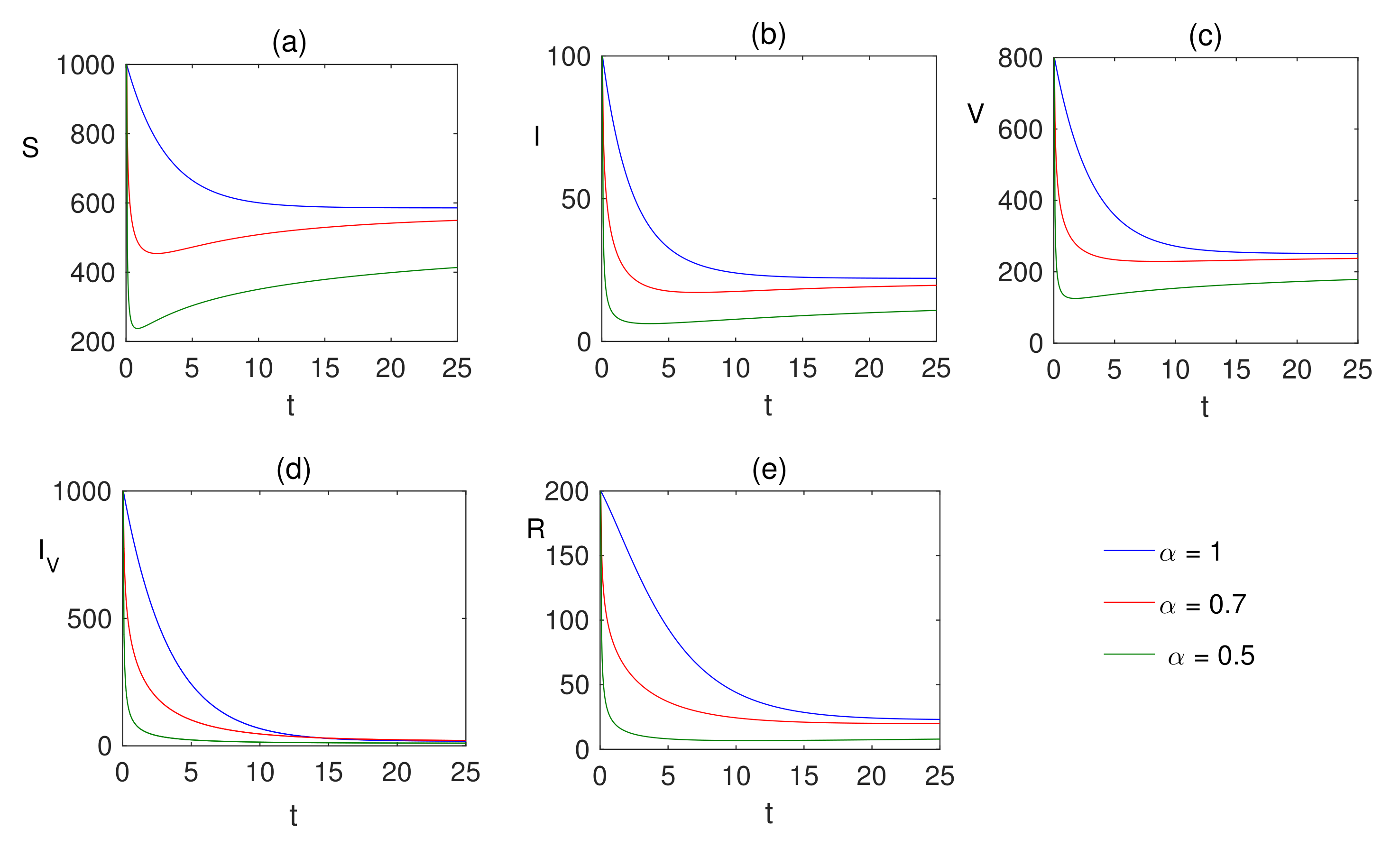
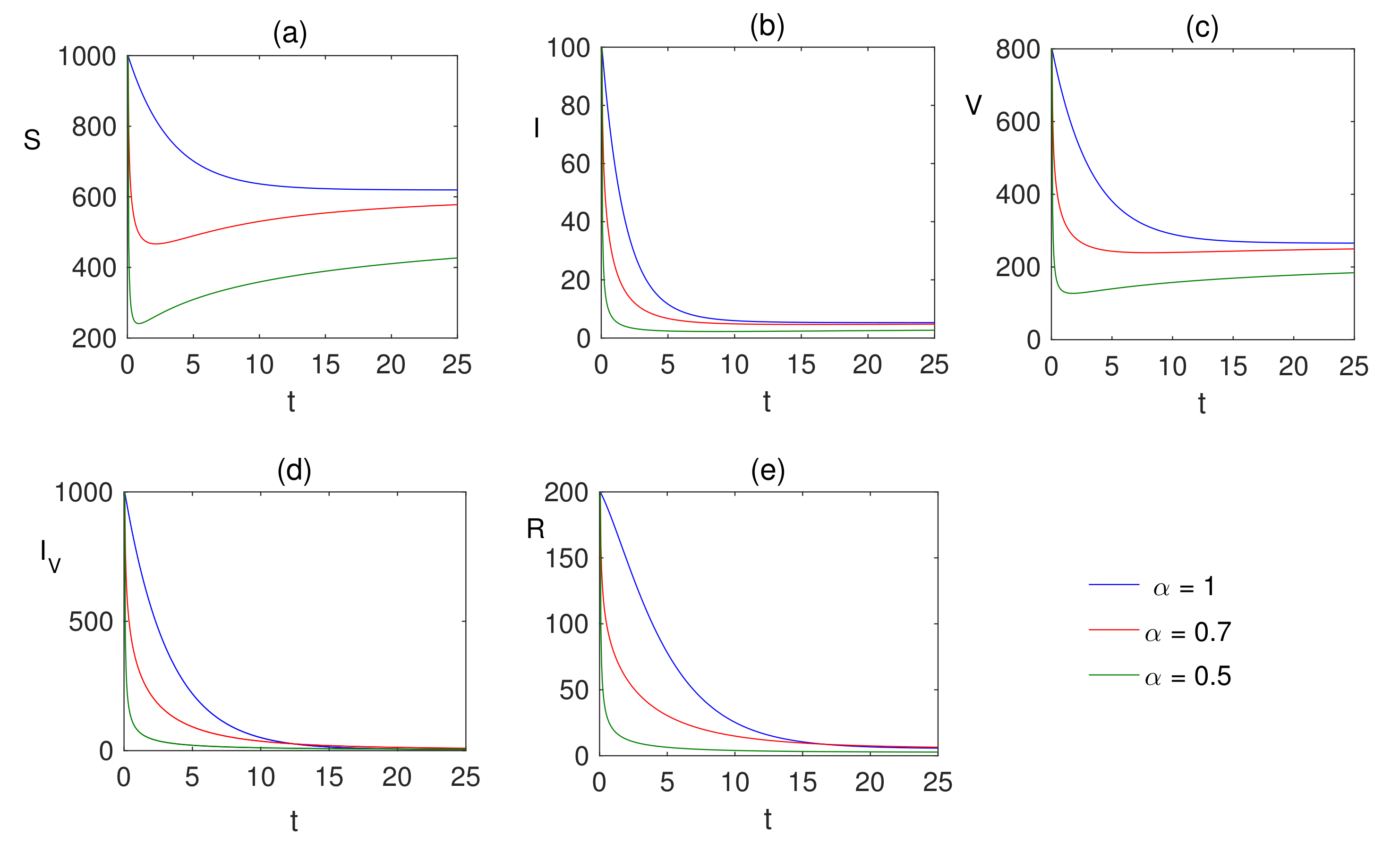
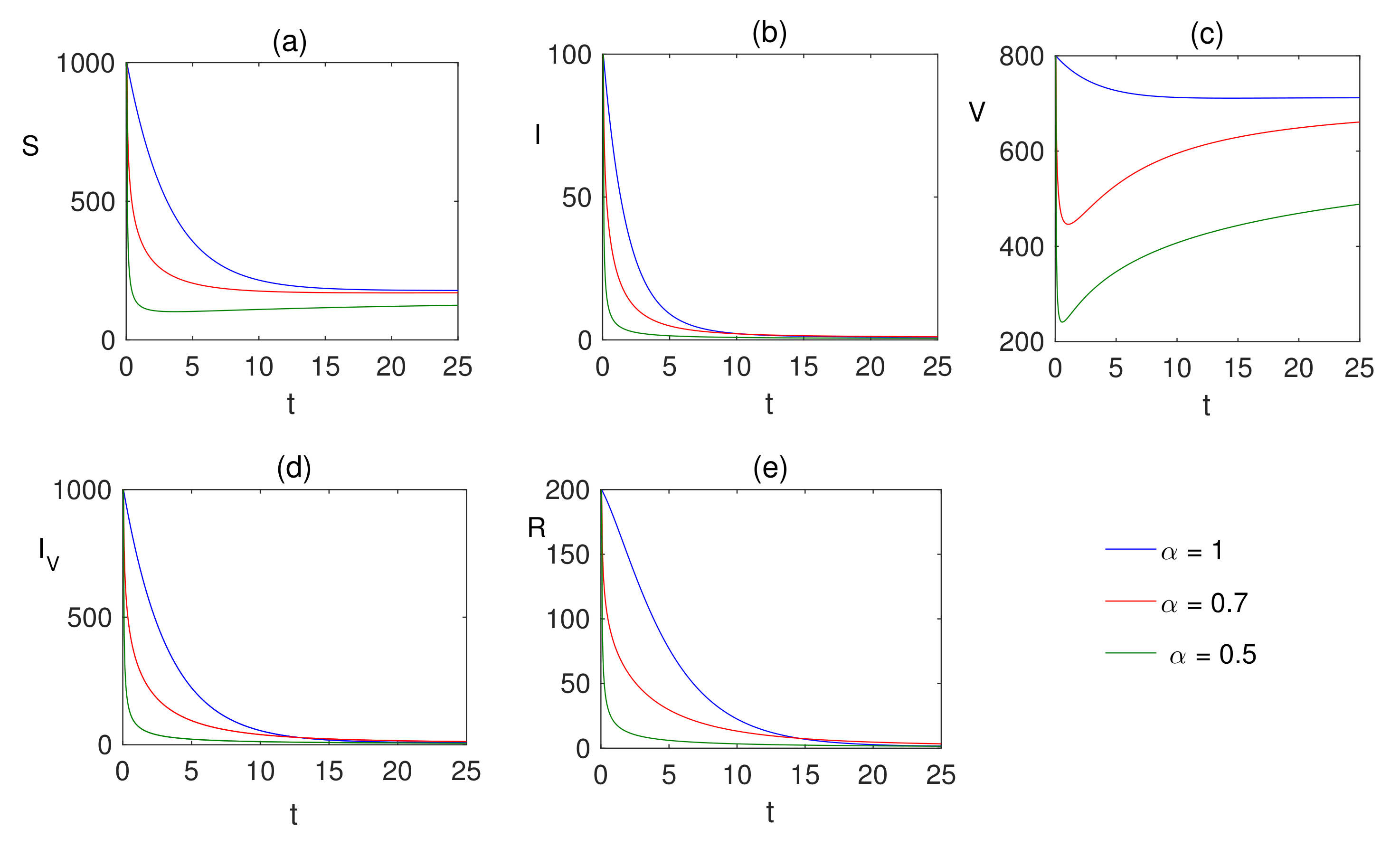
Comparison plots for the Caputo operators for different fear factors are provided in Figure 3 and Figure 4 considering various values of the fractional-order parameter $\alpha =1,0.7,0.5$; the graphical results are presented for comparison. By reducing the value of $\alpha$, it can be observed that the quantity of infected individuals declines. From these visual findings, ir can be noted that the fear factor for infection plays a crucial role in controlling the infection process, and helps with vaccination strategies as well. As the fear factor increases, the vaccinated population increases, and the infected population is simultaneously reduced.

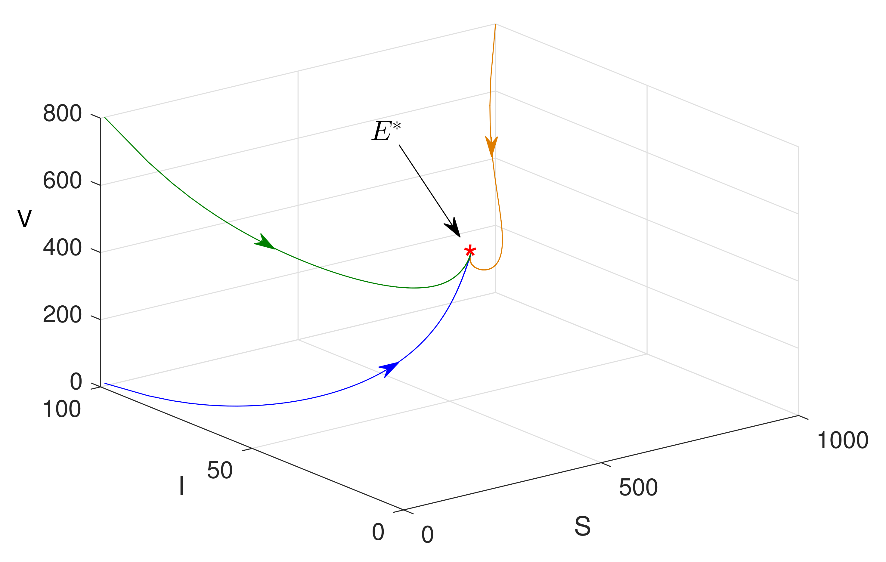
Figure 5 shows that the solution of system (7) is independent of initial conditions. Figure 5 shows that system (7) attains its globally asymptotic stability around the endemic equilibrium $E^{*}$ in $S-I-V$ phase space as different preliminary conditions taking the rest of the values of the parameters as in Table 1 where $R_0>1$.

7. Discussion

The anticipated benefits and efficacy of the vaccine need to be fully elaborated before introducing it. Mathematical modeling with the fractional derivative of population dynamics, including the effects of vaccination, can assist in disease management strategies. The basic reproduction number of the proposed model is important for the disease dynamics as well.

It has been observed that the proposed FDE model shows greater efficacy than the one exhibited by the integer-order model [5]. This study focuses on possible issues that may arise due to vaccination for COVID-19. Thus, the dynamics of the COVID-19 disease model in light of vaccination through a fractional differential equation (FDE) involving Caputo fractional derivative are presented here.

The existence and uniqueness of solutions for the proposed FDE model were obtained (Theorem 1). It can be seen that the solutions are independent of the choice of initial values of the model variables (Figure 5). The disease-free state is stable when $R_0<1$ (Figure 2), and this state can be obtained by decreasing infection rates. The numerical simulation for different values of the fractional-order parameter $\alpha =1,0.7,0.5$ are presented in (Figure 3, Figure 4, Figure 5 and Figure 6). In addition, the respective outcome of these choices are discussed. The comparison results for different fear factors are helpful for disease control policies, as the population of infected individuals can be decreased.

In summary, the proposed fractional-order model is highly functional for studying the dynamics of COVID-19 with vaccination. It can capture the psychological changes of the fear effects related to infection and the effects of vaccination on controlling COVID-19 infection. The obtained results are helpful in COVID-19 disease management. The present work can be extended using fractional optimal control theory [7,41] for greater cost-effectiveness of vaccination. Additionally, awareness programs through social media [44] can be included in this model to further improve outcomes.

References

- Biscayart, C.; Angeleri, P.; Lloveras, S.; Chaves, T.d.S.S.; Schlagenhauf, P.; Rodríguez-Morales, A.J. The next big threat to global health? 2019 novel coronavirus (2019-nCoV): What advice can we give to travellers?—Interim recommendations January 2020, from the Latin-American society for Travel Medicine (SLAMVI). Travel Med. Infect. Dis. 2020, 33, 101567. [Google Scholar] [CrossRef] [PubMed]
- Ahmad, S.; Ullah, A.; Al-Mdallal, Q.M.; Khan, H.; Shah, K.; Khan, A. Fractional order mathematical modeling of COVID-19 transmission. Chaos Solitons Fractals 2020, 139, 110256. [Google Scholar] [CrossRef] [PubMed]
- Sparrow, A.K.; Brosseau, L.M.; Harrison, R.J.; Osterholm, M.T. Protecting Olympic participants from Covid-19—The urgent need for a risk-management approach. N. Engl. J. Med. 2021, 385, e2. [Google Scholar] [CrossRef]
- Jamali, A.A. COVID-19 VACCINES. J. Peoples Univ. Med. Health Sci. Nawabshah (JPUMHS) 2020, 10, 1–2. [Google Scholar]
- Zou, L.; Ruan, F.; Huang, M.; Liang, L.; Huang, H.; Hong, Z.; Yu, J.; Kang, M.; Song, Y.; Xia, J.; et al. SARS-CoV-2 viral load in upper respiratory specimens of infected patients. N. Engl. J. Med. 2020, 382, 1177–1179. [Google Scholar] [CrossRef]
- Chatterjee, A.N.; Ahmad, B. A fractional-order differential equation model of COVID-19 infection of epithelial cells. Chaos Solitons Fractals 2021, 147, 110952. [Google Scholar] [CrossRef]
- Chatterjee, A.N.; Al Basir, F.; Almuqrin, M.A.; Mondal, J.; Khan, I. SARS-CoV-2 infection with lytic and non-lytic immune responses: A fractional order optimal control theoretical study. Results Phys. 2021, 26, 104260. [Google Scholar] [CrossRef]
- Mondal, J.; Samui, P.; Chatterjee, A.N. Optimal control strategies of non-pharmaceutical and pharmaceutical interventions for COVID-19 control. J. Interdiscip. Math. 2021, 24, 125–153. [Google Scholar] [CrossRef]
- Chatterjee, A.N.; Al Basir, F. A model for SARS-COV-2 infection with treatment. Comput. Math. Methods Med. 2020, 2020, 1352982. [Google Scholar] [CrossRef]
- Atangana, A. Modelling the spread of COVID-19 with new fractal-fractional operators: Can the lockdown save mankind before vaccination? Chaos Solitons Fractals 2020, 136, 109860. [Google Scholar] [CrossRef]
- Tang, B.; Wang, X.; Li, Q.; Bragazzi, N.L.; Tang, S.; Xiao, Y.; Wu, J. Estimation of the transmission risk of the 2019-nCoV and its implication for public health interventions. J. Clin. Med. 2020, 9, 462. [Google Scholar] [CrossRef] [PubMed] [Green Version]
- Sarkar, K.; Khajanchi, S.; Nieto, J.J. Modeling and forecasting the COVID-19 pandemic in India. Chaos Solitons Fractals 2020, 139, 110049. [Google Scholar] [CrossRef] [PubMed]
- Giordano, G.; Blanchini, F.; Bruno, R.; Colaneri, P.; Di Filippo, A.; Di Matteo, A.; Colaneri, M. Modelling the COVID-19 epidemic and implementation of population-wide interventions in Italy. Nat. Med. 2020, 26, 855–860. [Google Scholar] [CrossRef] [PubMed]
- Gatto, M.; Bertuzzo, E.; Mari, L.; Miccoli, S.; Carraro, L.; Casagrandi, R.; Rinaldo, A. Spread and dynamics of the COVID-19 epidemic in Italy: Effects of emergency containment measures. Proc. Natl. Acad. Sci. USA 2020, 117, 10484–10491. [Google Scholar] [CrossRef] [PubMed] [Green Version]
- Gumel, A.B.; Ruan, S.; Day, T.; Watmough, J.; Brauer, F.; Van den Driessche, P.; Gabrielson, D.; Bowman, C.; Alexander, M.E.; Ardal, S.; et al. Modelling strategies for controlling SARS outbreaks. Proc. R. Soc. Lond. Ser. B Biol. Sci. 2004, 271, 2223–2232. [Google Scholar] [CrossRef] [Green Version]
- Liu, Z.; Magal, P.; Seydi, O.; Webb, G. A COVID-19 epidemic model with latency period. Infect. Dis. Model. 2020, 5, 323–337. [Google Scholar] [CrossRef]
- Samui, P.; Mondal, J.; Khajanchi, S. A mathematical model for COVID-19 transmission dynamics with a case study of India. Chaos Solitons Fractals 2020, 140, 110173. [Google Scholar] [CrossRef]
- Guariglia, E. Riemann zeta fractional derivative—Functional equation and link with primes. Adv. Differ. Equ. 2019, 2019, 261. [Google Scholar] [CrossRef]
- Torres-Hernandez, A.; Brambila-Paz, F. An approximation to zeros of the Riemann zeta function using fractional calculus. arXiv 2020, arXiv:2006.14963. [Google Scholar] [CrossRef]
- Li, C.; Dao, X.; Guo, P. Fractional derivatives in complex planes. Nonlinear Anal. Theory Methods Appl. 2009, 71, 1857–1869. [Google Scholar] [CrossRef]
- Guariglia, E. Fractional calculus, zeta functions and Shannon entropy. Open Math. 2021, 19, 87–100. [Google Scholar] [CrossRef]
- Závada, P. Operator of fractional derivative in the complex plane. Commun. Math. Phys. 1998, 192, 261–285. [Google Scholar] [CrossRef] [Green Version]
- Khan, M.A.; Ullah, S.; Okosun, K.; Shah, K. A fractional order pine wilt disease model with Caputo–Fabrizio derivative. Adv. Differ. Equ. 2018, 2018, 410. [Google Scholar] [CrossRef]
- Ullah, S.; Khan, M.A.; Farooq, M. A fractional model for the dynamics of TB virus. Chaos Solitons Fractals 2018, 116, 63–71. [Google Scholar] [CrossRef]
- Diethelm, K. A fractional calculus based model for the simulation of an outbreak of dengue fever. Nonlinear Dyn. 2013, 71, 613–619. [Google Scholar] [CrossRef]
- DarAssi, M.H.; Safi, M.A.; Khan, M.A.; Beigi, A.; Aly, A.A.; Alshahrani, M.Y. A mathematical model for SARS-CoV-2 in variable-order fractional derivative. Eur. Phys. J. Spec. Top. 2022. [Google Scholar] [CrossRef]
- Asamoah, J.K.K.; Okyere, E.; Yankson, E.; Opoku, A.A.; Adom-Konadu, A.; Acheampong, E.; Arthur, Y.D. Non-fractional and fractional mathematical analysis and simulations for Q fever. Chaos Solitons Fractals 2022, 156, 111821. [Google Scholar] [CrossRef]
- Baleanu, D.; Abadi, M.H.; Jajarmi, A.; Vahid, K.Z.; Nieto, J. A new comparative study on the general fractional model of COVID-19 with isolation and quarantine effects. Alex. Eng. J. 2022, 61, 4779–4791. [Google Scholar] [CrossRef]
- Ahmed, I.; Baba, I.A.; Yusuf, A.; Kumam, P.; Kumam, W. Analysis of Caputo fractional-order model for COVID-19 with lockdown. Adv. Differ. Equ. 2020, 2020, 394. [Google Scholar] [CrossRef]
- Kozioł, K.; Stanisławski, R.; Bialic, G. Fractional-order sir epidemic model for transmission prediction of covid-19 disease. Appl. Sci. 2020, 10, 8316. [Google Scholar] [CrossRef]
- Ndaïrou, F.; Torres, D.F. Mathematical Analysis of a Fractional COVID-19 Model Applied to Wuhan, Spain and Portugal. Axioms 2021, 10, 135. [Google Scholar] [CrossRef]
- Noeiaghdam, S.; Micula, S.; Nieto, J.J. A Novel Technique to Control the Accuracy of a Nonlinear Fractional Order Model of COVID-19: Application of the CESTAC Method and the CADNA Library. Mathematics 2021, 9, 1321. [Google Scholar] [CrossRef]
- Li, C.; Zeng, F. Numerical Methods for Fractional Calculus; CRC Press: Boca Raton, FL, USA, 2015; Volume 24. [Google Scholar]
- Roy, A.K.; Basir, F.A.; Roy, P.K. A vivid cytokines interaction model on psoriasis with the effect of impulse biologic (TNF-alpha inhibitor) therapy. J. Theor. Biol. 2019, 474, 63–77. [Google Scholar] [CrossRef] [PubMed]
- Segel, L.; Slemrod, M. The quasi-steady-state assumption: A case study in perturbation. SIAM Rev. 1989, 31, 446–477. [Google Scholar] [CrossRef]
- Lin, W. Global existence theory and chaos control of fractional differential equations. J. Math. Anal. Appl. 2007, 332, 709–726. [Google Scholar] [CrossRef] [Green Version]
- Diekmann, O.; Heesterbeek, J.A.P.; Metz, J.A. On the definition and the computation of the basic reproduction ratio R 0 in models for infectious diseases in heterogeneous populations. J. Math. Biol. 1990, 28, 365–382. [Google Scholar] [CrossRef] [Green Version]
- Van den Driessche, P.; Watmough, J. Reproduction numbers and sub-threshold endemic equilibria for compartmental models of disease transmission. Math. Biosci. 2002, 180, 29–48. [Google Scholar] [CrossRef]
- Rihan, F.A.; Baleanu, D.; Lakshmanan, S.; Rakkiyappan, R. On Fractional SIRC Model with Salmonella Bacterial Infection. Abstr. Appl. Anal. 2014, 2014, 136263. [Google Scholar] [CrossRef] [Green Version]
- Ahmed, E.; El-Sayed, A.M.A.; El-Saka, H.A. On some Routh-Hurwitz conditions for fractional order differential equations and their applications in Lorenz, Ro¨ssler, Chua and Chen systems. Phys. Lett. A 2006, 358, 1–4. [Google Scholar] [CrossRef]
- Cao, X.; Datta, A.; Al Basir, F.; Roy, P.K. Fractional-order model of the disease psoriasis: A control based mathematical approach. J. Syst. Sci. Complex. 2016, 29, 1565–1584. [Google Scholar] [CrossRef]
- Ahmad, S.W.; Sarwar, M.; Rahmat, G.; Shah, K.; Ahmad, H.; Mousa, A.A.A. Fractional order model for the coronavirus (COVID-19) in Wuhan, China. Fractals 2021, 30, 2240007. [Google Scholar] [CrossRef]
- Spencer, J.; Shutt, D.; Moser, S.; Clegg, H.; Wearing, H.; Mukundan, H.; Manore, C. Epidemiological Parameter Review and Comparative Dynamics of Influenza, Respiratory Syncytial Virus, Rhinovirus, Human Coronavirus, and Adenovirus. medRxiv 2020. [Google Scholar] [CrossRef] [Green Version]
- Maji, C.; Al Basir, F.; Mukherjee, D.; Ravichandran, C.; Nisar, K. COVID-19 propagation and the usefulness of awareness based control measures: A mathematical model with delay. AIMS Math. 2022, 7, 12091–12105. [Google Scholar] [CrossRef]
Figure 1.
The flow diagram of the model (5).
Figure 2.
(a) The transcritical bifurcation diagram at is presented; (b) the value of the basic reproduction number () is shown when the disease transmission rate () and the virions production rate () are varied simultaneously. Other parameter values are taken from Table 1.
Figure 3.
Numerical solution of (a) susceptible , (b) infected , (c) vaccinated population , (d) infected population after vaccination and (e) recovered populations are plotted for showing the dynamics of the fractional model (7) when , and the fear factors are and .
Figure 4.
Numerical solution of (a) susceptible , (b) infected , (c) vaccinated population , (d) infected population after vaccination and (e) recovered populations are plotted for showing the dynamics of the fractional ordered model (7) when and the fear factors are and .
Figure 5.
Phase portrait in S–I–V plane for three different initial conditions. In this figure, ; others parameters are same as in Figure 4. Colored lines are obtained from three different initial conditions.
Figure 6.
The numerical solution of (a) susceptible , (b) infected , (c) vaccinated population , (d) infected population after vaccination and (e) recovered populations are plotted for showing the dynamics of the fractional ordered model (7) when and where the fear factors are and .