Condition Number and Clustering-Based Efficiency Improvement of Reduced-Order Solvers for Contact Problems Using Lagrange Multipliers

Abstract

This paper focuses on reduced-order modeling for contact mechanics problems treated by Lagrange multipliers. The high nonlinearity of the dual solutions lead to poor classical data compression. A hyper-reduction approach based on a reduced integration domain (RID) is considered. The dual reduced basis is the restriction to the RID of the full-order dual basis, which ensures the hyper-reduced model to respect the non-linearity constraints. However, the verification of the solvability condition, associated with the well-posedness of the solution, may induce an extension of the primal reduced basis without guaranteeing accurate dual forces. We highlight the strong link between the condition number of the projected contact rigidity matrix and the precision of the dual reduced solutions. Two efficient strategies of enrichment of the primal POD reduced basis are then introduced. However, for large parametric variation of the contact zone, the reachable dual precision may remain limited. A clustering strategy on the parametric space is then proposed in order to deal with piece-wise low-rank approximations. On each cluster, a local accurate hyper-reduced model is built thanks to the enrichment strategies. The overall solution is then deeply improved while preserving an interesting compression of both primal and dual bases.

1. Introduction

Variational inequalities (VI) arising from contact mechanics problem are still nowadays computationally expensive to solve. The size of the discrete full-order model (FOM) becomes rapidly prohibitive when accurate solutions are required. The issue of high computational cost has been widely studied for variational equality problems, and a common solution consists in using reduced order modeling (ROM) techniques. However, in case of contact VI problems, the application of such techniques is not straightforward. Indeed the non-smoothness of the contact constraints, especially the non-negativity of the contact pressure, remains a challenge for the adaptation of ROM methods.

A number of numerical methods, such as the penalty method or the augmented Lagrangian (AL) formulation, consist in building unconstrained minimization problems for solving contact. In this particular framework, as the main challenges related to ROM adaptation are circumvented, various reduced-order methods have been successfully applied, see [1,2,3] for the penalty method and [4,5,6] for the AL (or AL-like) formulation. However these kinds of contact formulations require numerical parameter adjustments to reach convergence. Concerning the penalty method, another disadvantage is that practically this method leads to some approximation of contact conditions (cf. interpenetration).

In counterpart, the Lagrange multipliers approach enables satisfying, precisely, surface contact conditions. The resulting contact problem is a saddle-point problem with primal (displacement) and dual (contact pressure) variables. The Lagrange multipliers physically represent the contact pressures (opposite of the contact forces) and must remain non-negative. This constraint avoids the use of the famous proper orthogonal decomposition (POD) snapshots method for the reduction of the dual basis. Hence, very few ROM methods have been applied to such problems. Their features mainly concern the construction of a reliable low-rank dual basis. We can distinguish approaches related to quasi-static contact problems to those related to dynamic contact problems.

Concerning the reduction of (quasi-)static contact problems, we can cite the extension of the reduced basis method [7], where the dual reduced basis is obtained by snapshots selection. This may lead to a low compressed reduced basis for a large parametric space. In [8], a projected-based method was proposed with a non-negative matrix factorization (NNMF) to obtain the reduced dual basis. The NNMF satisfies the positivity constraint but does not give a high compression rate [9]. In [10], the dual reduced basis is built through a cone-projected greedy algorithm, resulting in a better compression rate. However, this approach has not yet been verified outside the training set. Another strategy was proposed in [9], lying on hyper-reduction techniques. Such kinds of techniques [11,12,13,14] have shown their efficacy in reducing high-dimensional reconstruction required by non-linearity evaluations. Hence, in [9] a hyper-reduction method based on a reduced integration domain (RID) [15] was adapted to contact problems. The low-rank dual basis is then simply defined as the restriction of the full-order dual basis to the RID, naturally ensuring the non-negativity constraint and leading to precise dual forces on the RID. Moreover, this method ensures the verification of the full contact conditions inside the RID.

Concerning dynamic contact problems, the problem of building a reduced dual basis respecting the non-negativity was recently bypassed [16] through the use of the reduction of the primal variable to compute the Lagrange multipliers in an incremental way or [17] through the use of the linear complementarity programming method where only the primal variable is reduced.

In this work, we propose to improve the efficiency of the so-called hybrid hyper-reduced (HHR) method, the hyper-reduced method based on the RID introduced in [9], especially for large parametric variations of the contact zone. The consistency of the HHR approach has been proven in [9], lying on the solvability condition. Since high primal basis compression by POD is performed, this condition may not be initially respected. It was proposed in [9] to enrich the primal reduced basis with primal finite element (FE) shape functions while not respecting the solvability condition. However, the respect of the solvability condition is generally not sufficient to obtain accurate dual forces. No guideline was proposed in [9] for the choice of the FE shape functions to be added. Practically, for D-dimensional problems ($D>1$), it was proposed to add all primal FE shape functions lying on the contact zone in the reduced primal basis. For high-dimensional problems with large parametric variations, this strategy may compromise data compression.

In order to automatically and efficiently extend the reduced primal basis, we first highlight in this contribution the strong relation between the projected contact rigidity matrix condition number and the precision of the dual solutions obtained by the HHR method. Taking this relation into account, we propose two primal basis enrichment strategies aimed at improving the condition number of the projected contact rigidity matrix while respecting the solvability condition. These enrichment strategies are both based on a greedy algorithm. There are very few elements in the literature studying the relation between the condition number and precision of a ROM method. To the best of our knowledge, only [13] uses the condition number as a selection criterion for the sampling in the missing point estimation (MPE) method.

Secondly, as the enrichment strategy may significantly increase the size of the primal reduced basis, we propose a clustering strategy derived from [18] to treat contact problems with large parametric spaces. The clustering enables us to build local ROMs and, hence, to reduce high nonlinear (and non-smooth) problems in a piece-wise low-rank manner. The interested reader can refer to [18,19,20,21,22] for examples of local ROMs applied to hyper-reduction schemes. Here, the local ROMs are obtained by applying on each cluster the HHR method for contact problems with the condition number-based enrichment introduced in this paper.

The proposed strategies result in highly accurate dual (and primal) solutions with reduced bases of limited sizes even for large variations of the contact zone.

The rest of the article is structured as follows. A brief presentation of the FOM for Lagrange multiplier-based contact problems is written in Section 2. The HHR model for contact mechanics is also recalled (and few adapted) in this section. In Section 3, we present the correlation between condition number of the projected contact rigidity matrix and precision of dual solutions. We then propose the two primal reduced basis enrichment strategies. In Section 4, the clustering framework for contact mechanics is introduced. Finally, in Section 5, numerical experiments are performed allowing to appreciate the efficiency of the proposed strategies.

2. Contact Problem, FE, and HHR Models

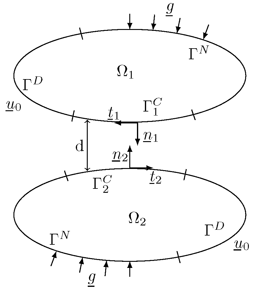
2.1. Static Unilateral Contact Problem

We are interested in the solution of elastostatic frictionless unilateral contact problems. The notations we consider are presented in Figure 1. Moreover, we classically denote by $u_N$ the relative normal displacement on the potential contact surface ${\Gamma }^C$, d the initial gap, and $F_N$ the normal force component. Then, the Signorini’s law for unilateral contact is given on ${\Gamma }^C$ by: the non-penetration condition $u_N\le d$, the non-adhesion condition $F_N\le 0$, and the complementarity slackness $(u_N-d)F_N=0$.

Under the small strain hypotheses, the strong formulation of the elastostatic frictionless unilateral contact problem can be expressed as [23,24,25]:

$$\left\{\begin{array}{cccc}\hfill -div\underset{\underset{¯}{¯}}{\sigma }=& \underset{¯}{f}\hfill & \hfill & in\Omega ,\hfill \\ \hfill \underset{\underset{¯}{¯}}{\sigma }=& \underset{\underset{\underset{¯}{¯}}{\underset{¯}{¯}}}{C}:\underset{\underset{¯}{¯}}{\epsilon }\hfill & \hfill & in\Omega ,\hfill \\ \hfill \underset{\underset{¯}{¯}}{\epsilon }=& \frac{1}{2}\left(grad\underset{¯}{u}+{(grad\underset{¯}{u})}^T\right)\hfill & \hfill & in\Omega ,\hfill \\ \hfill \underset{¯}{u}=& {\underset{¯}{u}}_0\hfill & \hfill & on{\Gamma }^D,\hfill \\ \hfill \underset{\underset{¯}{¯}}{\sigma }\underset{¯}{n}=& \underset{¯}{g}\hfill & \hfill & on{\Gamma }^N,\hfill \\ \hfill \underset{\underset{¯}{¯}}{\sigma }\underset{¯}{n}& F_N\underset{¯}{n}\hfill & \hfill & on{\Gamma }^C,\hfill \\ \hfill u_N\le d,F_N\le 0,& (d-u_N)F_N=0\hfill & \hfill & on{\Gamma }^C,\hfill \end{array}\right.$$

(1)

with $\underset{¯}{u}$ the displacement field, $\underset{\underset{¯}{¯}}{\sigma }$ the stress field, $\underset{\underset{¯}{¯}}{\epsilon }$ the strain field, $\underset{¯}{f}$ the prescribed volume density of forces, ${\underset{¯}{u}}_0$ the imposed displacement on ${\Gamma }^D$, $\underset{¯}{g}$ the imposed forces (surface density) on ${\Gamma }^N$, and $\underset{¯}{n}$ the external unit normal. The tensor $\underset{\underset{\underset{¯}{¯}}{\underset{¯}{¯}}}{C}$ denotes the fourth-order elasticity tensor.

The weak formulation derived from problem (1) induces a variational inequality (VI) [23]. This VI, equivalent to a minimization problem, can be classically treated by Lagrange multipliers [24]. The resulting weak formulation is then a saddle-point problem, cf. Equation (2).

$$\left\{\begin{array}{c}\mathrm{Find}(\underset{¯}{u},\lambda )\in \mathcal{V}\times \mathcal{W}\mathrm{such}\mathrm{that}\hfill \\ \begin{array}{cccc}\hfill a(\underset{¯}{u},\underset{¯}{v})+b(\underset{¯}{v},\lambda )& =l\left(v\right)\hfill & \hfill & \forall v\in {\mathcal{V}}_0,\hfill \\ \hfill b(\underset{¯}{u},q-\lambda )& \le {〈d,q-\lambda 〉}_{H^{\frac{1}{2}}\left({\Gamma }^C\right),H^{-\frac{1}{2}}\left({\Gamma }^C\right)}\hfill & \hfill & \forall q\in \mathcal{W},\hfill \end{array}\hfill \end{array}\right.$$

(2)

with $\lambda$ the Lagrange multiplier, $\mathcal{W}=\{q\in H^{-\frac{1}{2}}\left({\Gamma }^C\right)|q\ge 0\}$, $H^{-\frac{1}{2}}$ the dual of $H^{\frac{1}{2}}$, $b(\underset{¯}{v},q)={〈v_N,q〉}_{H^{\frac{1}{2}}\left({\Gamma }^C\right),H^{-\frac{1}{2}}\left({\Gamma }^C\right)}$ and ${〈·,·〉}_{H^{\frac{1}{2}},H^{-\frac{1}{2}}}$ the dual product, $\mathcal{V}=\{\underset{¯}{v}=\underset{¯}{r}\left({\underset{¯}{u}}_0\right)+\underset{¯}{\tilde{u}}|\underset{¯}{\tilde{u}}\in {\mathcal{V}}_0\}$, $\underset{¯}{r}\left({\underset{¯}{u}}_0\right)$ the lifting of ${\underset{¯}{u}}_0$ over $\Omega$, ${\mathcal{V}}_0=\{\underset{¯}{v}\in {\left(H^1(\Omega )\right)}^D|\underset{¯}{v}=\underset{¯}{0}sur{\Gamma }^D\}$ and

$$\begin{array}{c}\hfill a(\underset{¯}{u},\underset{¯}{v})={\int }_{\Omega }\underset{\underset{¯}{¯}}{\epsilon }\left(\underset{¯}{v}\right):\underset{\underset{\underset{¯}{¯}}{\underset{¯}{¯}}}{C}:\underset{\underset{¯}{¯}}{\epsilon }\left(\underset{¯}{u}\right)\mathrm{d}\Omega ,l\left(\underset{¯}{v}\right)={\int }_{\Omega }{\underset{¯}{f}}^T\underset{¯}{v}\mathrm{d}\Omega +{\int }_{{\Gamma }^N}{\underset{¯}{g}}^T\underset{¯}{v}\mathrm{d}\Gamma .\end{array}$$

2.2. Finite Element Discretization

The standard FE discretization [25] of the saddle-point problem (2) results in system (3).

$$\left\{\begin{array}{c}\mathrm{Find}(\underset{¯}{U},\underset{¯}{\Lambda })\in {\mathbb{R}}^N\times {\left({\mathbb{R}}^{+}\right)}^{N_{\lambda }}\mathrm{such}\mathrm{that}\hfill \\ \begin{array}{cc}\hfill \underset{\underset{¯}{¯}}{K}\underset{¯}{U}+{\underset{\underset{¯}{¯}}{B}}^T\underset{¯}{\Lambda }& =\underset{¯}{F},\hfill \\ \hfill \underset{\underset{¯}{¯}}{B}\underset{¯}{U}& \le \underset{¯}{D},\hfill \\ \hfill {\underset{¯}{\Lambda }}^T(\underset{¯}{D}-\underset{\underset{¯}{¯}}{B}\underset{¯}{U})& =0,\hfill \end{array}\hfill \end{array}\right.$$

(3)

with U being the discretization of the displacement solution in the primal FE basis, $\underset{¯}{\Lambda }$ the discretization of the Lagrange multipliers in the dual FE basis, N is the number of primal DoFs, and $N_{\lambda }$ is the number of potential contacts. The matrices or vectors $\underset{\underset{¯}{¯}}{K}\in {\mathbb{R}}^{N\times N}$; $\underset{\underset{¯}{¯}}{B}\in {\mathbb{R}}^{N_{\lambda }\times N}$; $\underset{¯}{F}\in {\mathbb{R}}^N$, $\underset{¯}{D}\in {\mathbb{R}}^{N_{\lambda }}$ are respectively the rigidity matrix, the contact rigidity matrix, the source vector and the initial gap vector.

The discrete saddle-point problem (3) has to respect the classical Ladyzhenskaya–Babuška–Brezzi (LBB) [26,27] or inf–sup condition implying stability of the solution and, hence, solvability of the problem. For node-to-node contact with linear (or bilinear) finite element approximations, which are of interest here, this condition is ensured [28].

2.3. Hybrid Hyper-Reduced Model

2.3.1. Reduced Integration Domain for Contact Problems

The RID [15], which will be the support of the hyper-reduced discretized problem, is built from a set of DoFs associated to nodes located on the whole domain $\Omega$. The DoF selection method usually consists of a sampling method, such as the DEIM [12] or an arbitrary selection for areas of interest.

For contact problems, the RID definition must be adapted to ensure computable gaps on the RID. We focus here on the node-to-node contact algorithm. In [9], an extension of the RID interface has been proposed, see Figure 2a. The unpaired DoFs on the potential contact surface of the RID were hence removed from the set of available balance equations. In this paper, we propose an extension of the RID to treat contact on each node of the potential contact zone included in the RID, see Figure 2b. Denoting by $\mathcal{L}$, the list of node indices used to build the RID, the complementary contact list ${\mathcal{L}}^{\prime }$ reads

$${\mathcal{L}}^{\prime }=\{\mathrm{node}j\mathrm{on}{\Gamma }^C;j\notin \mathcal{L}|\exists i\in \mathcal{L}\mathrm{such}\mathrm{that}(i,j)\mathrm{is}\mathrm{a}\mathrm{pair}\mathrm{of}\mathrm{contact}\mathrm{nodes}\}.$$

(4)

The RID is now defined as:

$${\Omega }_A=\left(\bigcup _{i\in \mathcal{L}}\mathrm{supp}\left({\underset{¯}{\phi }}_i\right)\right)\bigcup \left(\bigcup _{j\in {\mathcal{L}}^{\prime }}\mathrm{supp}\left({\underset{¯}{\phi }}_j\right)\right),$$

(5)

with ${\underset{¯}{\phi }}_k$, $k=1,\dots ,N$ the FE shape functions.

We denote ${\Omega }_B$ as the counterpart of ${\Omega }_A$ such that $\Omega ={\Omega }_A\cup {\Omega }_B$. The complementary list ${\mathcal{L}}^{\prime }$ plays the role of a zone of interest as defined in [15]. This construction variation allows to deal with more potential contacts, but slightly enlarges the size of the RID.

2.3.2. Reduced Bases

Concerning the primal basis reduction, the standard POD-snapshot method [29] is used. The size l of this reduced basis (RB) is automatically obtained according to the approximation error ${ϵ}_{\mathcal{POD}}$ on the snapshot matrix. The primal RB is then the matrix $\underset{\underset{¯}{¯}}{V}\in {\mathbb{R}}^{N\times l}$ containing the l first left singular vectors of the singular value decomposition (SVD) of the snapshots matrix. The discrete displacement is then projected in this RB $\underset{¯}{U}=\underset{\underset{¯}{¯}}{V}\underset{¯}{\gamma }$, $\underset{¯}{\gamma }\in {\mathbb{R}}^l$ being degrees of freedom (DoFs) associated to the primal RB, $l\ll N$.

In order to avoid a non efficient compression of the dual basis, we used the RID concept to simply reduce the number of dual DoFs by restriction of the dual FOM basis to the RID. This strategy enables precise dual forces to be obtained on the RID, as shown in [9].

In counterpart, the reduced dual basis is of local support only. If the solution outside the RID is of interest, a reconstruction strategy based on the solution of a non-negative least squares (NNLS) problem using the dual snapshots, as well as the ROM primal and dual solutions, was proposed in [9].

2.3.3. Hybrid Hyper-Reduced Formulation

Complexity reduction of hyper-reduced models accounts for the sparsity of finite element matrices. We introduce the set $\mathcal{A}$ of primal DoFs not connected to ${\Omega }_B$:

$$\mathcal{A}=\left\{i\in \left[[1,N]\right]|{\int }_{{\Omega }_B}{\underset{¯}{\phi }}_i^T{\underset{¯}{\phi }}_{i}d\Omega =0\right\},$$

(6)

and the set $\mathcal{I}$ of DoFs connected to $\mathcal{A}$ by the rigidity matrix $\underset{\underset{¯}{¯}}{K}$ (interface nodes in the discretization scheme sense):

$$\mathcal{I}=\left\{{j\in \left[[1,N]\right],j\notin \mathcal{A}|\exists i\in \mathcal{A}\mathrm{s.t.}\left(\underset{\underset{¯}{¯}}{K}\right)}_{ij}\ne 0\right\}.$$

(7)

Concerning the reduction of the contact conditions, we define the set ${\mathcal{A}}_c$ of DoFs of $\mathcal{A}$ localized on the potential contact zone and the set ${\mathcal{A}}_{\lambda }$ of dual DoFs connected to ${\mathcal{A}}_c$ by the contact matrix $\underset{\underset{¯}{¯}}{B}$.

$$\begin{array}{cc}\hfill {\mathcal{A}}_c& =\{j\in \mathcal{A}|\exists i\in \left[[1,N_{\lambda }]\right]\mathrm{s.t.}{\left(\underset{\underset{¯}{¯}}{B}\right)}_{ij}\ne 0\},\hfill \end{array}$$

(8)

$$\begin{array}{cc}\hfill {\mathcal{A}}_{\lambda }& =\{i\in \left[[1,N_{\lambda }]\right]|\exists j\in {\mathcal{A}}_c\mathrm{s.t.}{\left(\underset{\underset{¯}{¯}}{B}\right)}_{ij}\ne 0\}.\hfill \end{array}$$

(9)

The cardinal of ${\mathcal{A}}_{\lambda }$, denoted $N_{\lambda }^C$ in the sequel, corresponds to the number of potential contact points in the RID and, hence, to the size of the dual reduced basis. The hybrid hyper-reduced (HHR) model, introduced in [9], reads:

$$\left\{\begin{array}{c}\mathrm{Find}(\underset{¯}{\gamma },\underset{¯}{\Lambda })\in {\mathbb{R}}^l\times {\left({\mathbb{R}}^{+}\right)}^{N_{\lambda }^C}\mathrm{such}\mathrm{that}\hfill \\ \begin{array}{cc}\hfill \underset{\underset{¯}{¯}}{V}{[\mathcal{A},:]}^T\underset{\underset{¯}{¯}}{K}[\mathcal{A},\mathcal{A}\cup \mathcal{I}]\underset{\underset{¯}{¯}}{V}[\mathcal{A}\cup \mathcal{I},:]\underset{¯}{\gamma }+\underset{\underset{¯}{¯}}{V}{[{\mathcal{A}}_c,:]}^T\underset{\underset{¯}{¯}}{B}{[{\mathcal{A}}_{\lambda },{\mathcal{A}}_c]}^T\underset{¯}{\Lambda }\left[{\mathcal{A}}_{\lambda }\right]& =\underset{\underset{¯}{¯}}{V}{[\mathcal{A},:]}^T\underset{¯}{F}\left[\mathcal{A}\right],\hfill \\ \hfill \underset{\underset{¯}{¯}}{B}[{\mathcal{A}}_{\lambda },{\mathcal{A}}_c]\underset{\underset{¯}{¯}}{V}[{\mathcal{A}}_c,:]\underset{¯}{\gamma }& \le \underset{¯}{D}\left[{\mathcal{A}}_{\lambda }\right],\hfill \\ \hfill \underset{¯}{\Lambda }{\left[{\mathcal{A}}_{\lambda }\right]}^T(\underset{¯}{D}\left[{\mathcal{A}}_{\lambda }\right]-\underset{\underset{¯}{¯}}{B}[{\mathcal{A}}_{\lambda },{\mathcal{A}}_c]\underset{\underset{¯}{¯}}{V}[{\mathcal{A}}_c,:]\underset{¯}{\gamma })& =0,\hfill \end{array}\hfill \end{array}\right.$$

(10)

with $\underset{¯}{\gamma }$ being the primal solution and $\underset{¯}{\Lambda }\left[{\mathcal{A}}_{\lambda }\right]$ the dual solution of the reduced model. As shown in Equation (10), the HHR formulation respects all of Signorini’s conditions inside the RID.

As Problem (3), Problem (10) is a saddle-point problem. It was proven in [9] that the HHR formulation is consistent with the FE formulation if the solvability condition of Problem (10) is respected. In the setting of (10), it leads to have $\underset{\underset{¯}{¯}}{B}[{\mathcal{A}}_{\lambda ,\mathrm{active}},{\mathcal{A}}_c]\underset{\underset{¯}{¯}}{V}[{\mathcal{A}}_c,:]$ of full row rank, ${\mathcal{A}}_{\lambda ,\mathrm{active}}$ being the set of DoFs associated to an active contact (equality constraint), which is a priori unknown.

3. Solvability Condition and Enrichment of the Primal Reduced Basis

3.1. Extended Solvability Condition

The set of active contact ${\mathcal{A}}_{\lambda ,\mathrm{active}}$ being a priori unknown, we have to consider a stronger solvability-like condition. We impose the projected contact rigidity matrix, including all potential contacts, i.e., $\underset{\underset{¯}{¯}}{B}[{\mathcal{A}}_{\lambda },{\mathcal{A}}_c]\underset{\underset{¯}{¯}}{V}[{\mathcal{A}}_c,:]$, to be of full row rank. Since $\underset{\underset{¯}{¯}}{B}$ contains as many lines as there are potential contact points (node-to-node contact), the extended solvability condition on the reduced model (10) imposes

$$\mathrm{rank}\left(\underset{\underset{¯}{¯}}{B}[{\mathcal{A}}_{\lambda },{\mathcal{A}}_c]\underset{\underset{¯}{¯}}{V}[{\mathcal{A}}_c,:]\right)=N_{\lambda }^C.$$

(11)

A necessary condition to verify Equation (11) is that $N_{\lambda }^C\le l$, which is not always respected due to the RID construction. In order to respect Condition (11) without modifying the RID, the primal RB has to be enriched.

In [9], it was proposed to enrich the primal RB with FE shape functions related to the nodes on the contact surface. In the case of Lagrange FE, the extended primal RB denoted $\overline{\underset{\underset{¯}{¯}}{V}}$ then reads:

$$\overline{\underset{\underset{¯}{¯}}{V}}=\left(\underset{\underset{¯}{¯}}{V}{\underset{\underset{¯}{¯}}{I}}_N\left[:,{\mathcal{L}}_C\right]\right),$$

(12)

with ${\underset{\underset{¯}{¯}}{I}}_N$, the identity matrix of size N, ${\mathcal{L}}_C\subset {\mathcal{A}}_C$ the node indices of the FE shape functions to be added. The primal reduced basis dimension is then $\overline{l}=l+card\left({\mathcal{L}}_C\right)$. This enrichment is advantageous to accurately solve the solution on the contact surface, but the choice of ${\mathcal{L}}_C$ may be not trivial. In [9], the enrichment was either done manually with an arbitrary selection (for one-dimensional problems) or it was proposed to add all primal FE shape functions of the potential contact zone in order to simply ensure the full row rank condition, good stability, and accurate solutions on the contact zone. In this latter case, ${\mathcal{L}}_C={\mathcal{A}}_C$, which may lead to a significant expansion of the primal RB.

One of the main contributions of this paper includes strategies to automatically and wisely obtain the set ${\mathcal{L}}_C$ in order to optimize the ratio between the primal RB dimension $\overline{l}$ and the precision of the dual-reduced solutions.

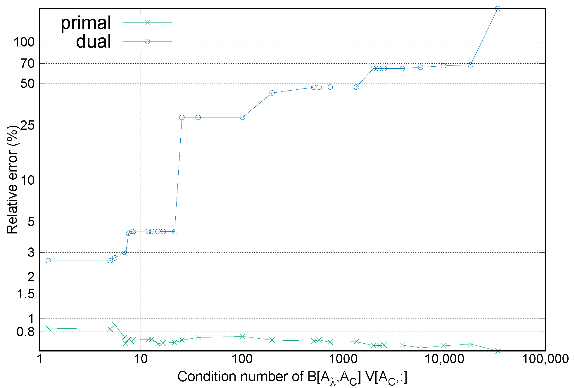
3.2. Importance of the Projected Contact Rigidity Matrix Condition Number

In the FE model, the condition number of the contact rigidity matrix $\underset{\underset{¯}{¯}}{B}$, written $\kappa \left(\underset{\underset{¯}{¯}}{B}\right)$, is equal to 1. According to this observation, the more the condition number of the projected contact rigidity matrix of the HHR model, denoted $\kappa \left(\underset{\underset{¯}{¯}}{B}[{\mathcal{A}}_{\lambda },{\mathcal{A}}_c]\underset{\underset{¯}{¯}}{V}[{\mathcal{A}}_c,:]\right)$, is close to 1, the more precise the dual reduced solutions. On the other hand, the primal reduced solutions are less sensitive to this condition number. An illustration of this behaviour of dual and primal HHR solutions are reported in Figure 3, from the test case of Section 5.2. The relative errors considered are presented in Section 5.1, Equations (17) (primal) and (18) (dual).

3.3. FE Enrichment of the Primal RB

In order to make the condition number $\kappa \left(\underset{\underset{¯}{¯}}{B}[{\mathcal{A}}_{\lambda },{\mathcal{A}}_c]\underset{\underset{¯}{¯}}{V}[{\mathcal{A}}_c,:]\right)$ closer to $\kappa \left(\underset{\underset{¯}{¯}}{B}\right)$, it seems natural to add to the primal RB $\underset{\underset{¯}{¯}}{V}$ some FE shape functions located on the potential contact zone of the RID, cf. Equation (12). When ${\mathcal{L}}_C={\mathcal{A}}_C$, we then have $\kappa \left(\underset{\underset{¯}{¯}}{B}[{\mathcal{A}}_{\lambda },{\mathcal{A}}_c]\overline{\underset{\underset{¯}{¯}}{V}}[{\mathcal{A}}_c,:]\right)=\kappa \left(\underset{\underset{¯}{¯}}{B}\right)$.

We propose to automatically obtain the set ${\mathcal{L}}_C\subset {\mathcal{A}}_C$ through a greedy algorithm based on $\kappa \left(\underset{\underset{¯}{¯}}{B}[{\mathcal{A}}_{\lambda },{\mathcal{A}}_c]\overline{\underset{\underset{¯}{¯}}{V}}[{\mathcal{A}}_c,:]\right)$, see Algorithm 1. In this algorithm, ${\mathcal{A}}_C\left(p\right)$ denotes the DoF number associated to the $p^{th}$ element of ${\mathcal{A}}_C$.

Algorithm 1: Greedy algorithm based on the condition number of the projected contact rigidity matrix to enrich the primal RB.

It is worth noting that even when the extended solvability condition is respected, the set ${\mathcal{L}}_C$ could continue to be enlarged in order to improve the dual solutions.

3.4. POD Modes and FE Shape Functions Enrichment of the Primal RB

The FE shape function enrichment is a way to extend the primal RB, but it naturally comes to mind to use an enrichment strategy that uses more POD modes (less truncated SVD) for a given RID. In this way, more global information (from snapshots) can be included in the extended primal RB.

Practically, this strategy is based on a second POD threshold ${ϵ}_{\mathcal{POD}2}<{ϵ}_{\mathcal{POD}}$ to obtain $l_2$ supplementary primal POD modes. The primal POD basis considered in the HHR model (10) is now $\underset{\underset{¯}{¯}}{V}\in {\mathbb{R}}^{N\times (l+l_2)}$.

The extension of the primal POD RB through the order of singular vectors does not guarantee the extended solvability condition or a satisfying condition number of the projected contact rigidity matrix. Hence, this strategy has to be combined with the FE shape function enrichment (see Section 3.3 and Algorithm 1) to obtain accurate dual solutions.

The main advantage of this strategy is that it allows us to use a more precise POD RB without impacting the size of the RID. Indeed, in most cases, the RID construction is based on a selection method relying on the primal RB (running the DEIM algorithm on the primal RB for example). Hence, there is a strong connection between the size of the primal RB and the size of the RID. Using the proposed strategy, the RID construction is still based on the POD threshold ${ϵ}_{\mathcal{POD}}$ while the HHR model is based on the extended POD threshold ${ϵ}_{\mathcal{POD}2}$. Let us underline that ${ϵ}_{\mathcal{POD}2}$ must remain large enough in order to avoid overfitting. Hence, this strategy is mainly of interest for large parametric spaces.

Remark 1. 

For both enrichment strategies, one has to verify the basis property of the extended matrix $\overline{\underset{\underset{¯}{¯}}{V}}$ on the RID. The verification has to be done in the offline part of the method, without impacting the online part.

4. Clustering

In case of highly nonlinear problems, such as non-smooth contact problems, clustering strategies may offer the possibly of treating the nonlinearity in a linear piece-wise manner through low-rank (ROM) approximations on different clusters partitioning the parametric space [18]. For large parametric spaces, we then expect to improve the accuracy of the reduced solution for a given dimension of RBs.

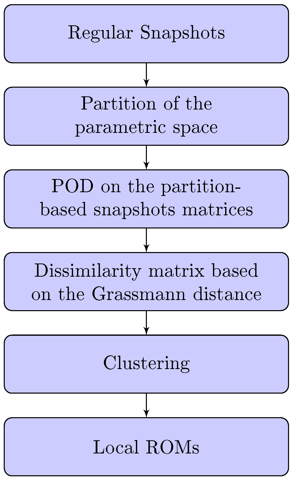
4.1. From Regular Snapshots

The framework of the clustering strategy is presented in Figure 4. The training set ${\mathcal{P}}_{tr}$ is generated through a regular discretization of the training space $\mathcal{P}$. FOM primal snapshots are calculated on the parametric points of ${\mathcal{P}}_{tr}$.

We then consider a partition of $\mathcal{P}$ composed of $N_s$ elements relying on the discretization ${\mathcal{P}}_{tr}$. On each element $j=1,\dots ,N_s$, an orthonormal basis ${\underset{\underset{¯}{¯}}{V}}_j$ is obtained from the POD on the element-wise snapshot matrix. This local snapshot matrix is composed by snapshots associated to points in ${\mathcal{P}}_{tr}$ belonging to element j.

As suggested in [18,30], the Grassmann distance $d_{Gr(\infty ,\infty )}$ between local RBs is then used for the clustering of the simulated data for model order reduction. The dissimilarity matrix $\underset{\underset{¯}{¯}}{\delta }\in {\mathbb{R}}^{M_s\times M_s}$ writes:

$$\forall j_1,j_2\in {\left[[0,N_s]\right]}^2,{\left(\underset{\underset{¯}{¯}}{\delta }\right)}_{j_1,j_2}=d_{Gr(\infty ,\infty )}({\underset{\underset{¯}{¯}}{V}}_{j_1},{\underset{\underset{¯}{¯}}{V}}_{j_2}),$$

(13)

with

$$d_{Gr(\infty ,\infty )}({\underset{\underset{¯}{¯}}{A}}_1,{\underset{\underset{¯}{¯}}{A}}_2)={\left(\frac{{\pi }^2}{4}|a_1-a_2|+\sum _{i=1}^{min(a_1,a_2)}{\alpha }_i^2\right)}^{\frac{1}{2}},$$

(14)

where $a_1$ and $a_2$ are the dimensions of bases ${\underset{\underset{¯}{¯}}{A}}_1$ and ${\underset{\underset{¯}{¯}}{A}}_2$, respectively. The angles ${\alpha }_i$ are related to the singular values ${\Sigma }_{ii},1<i\le min(a_1,a_2)$, of ${\underset{\underset{¯}{¯}}{A}}_1^T{\underset{\underset{¯}{¯}}{A}}_2$ by Equation (15)

$${\Sigma }_{ii}=cos\left({\alpha }_i\right).$$

(15)

The smaller ${\left(\underset{\underset{¯}{¯}}{\delta }\right)}_{j_1,j_2}$, the closer the subspace spanned by bases ${\underset{\underset{¯}{¯}}{V}}_{j_1}$ and ${\underset{\underset{¯}{¯}}{V}}_{j_2}$, separately. A clustering algorithm based on the dissimilarity matrix $\underset{\underset{¯}{¯}}{\delta }$ is finally applied to build K clusters from the initial partition of $\mathcal{P}$ into $N_s$ elements. In this work, we use the k-medoids algorithm [31], to focus on compactness.

On each cluster k, $k=1,\dots ,\underset{\underset{¯}{¯}}{K}$, the local snapshots matrix gathers the snapshots associated to points of the training set ${\mathcal{P}}_{tr}$ included into the cluster. From this local snapshots matrix, a local HHR model is built following the strategy described in Section 2.3. In particular, a local RID is considered in each cluster k.

As the clustering aims to reduce the range of the parameter variations, an accurate low-rank approximation of the primal basis can be obtained. Hence, in this case, only the enrichment strategy based on FE shape functions (see Section 3.3) has to be considered in order to ensure both the respect of the local solvability condition as well as accurate reduced dual forces.

Concerning the classification, a trivial strategy based on the clustering partition of the parametric space $\mathcal{P}$ is used. This classification is used online for the local ROM selection associated to given input data (generally outside the training set ${\mathcal{P}}_{tr}$).

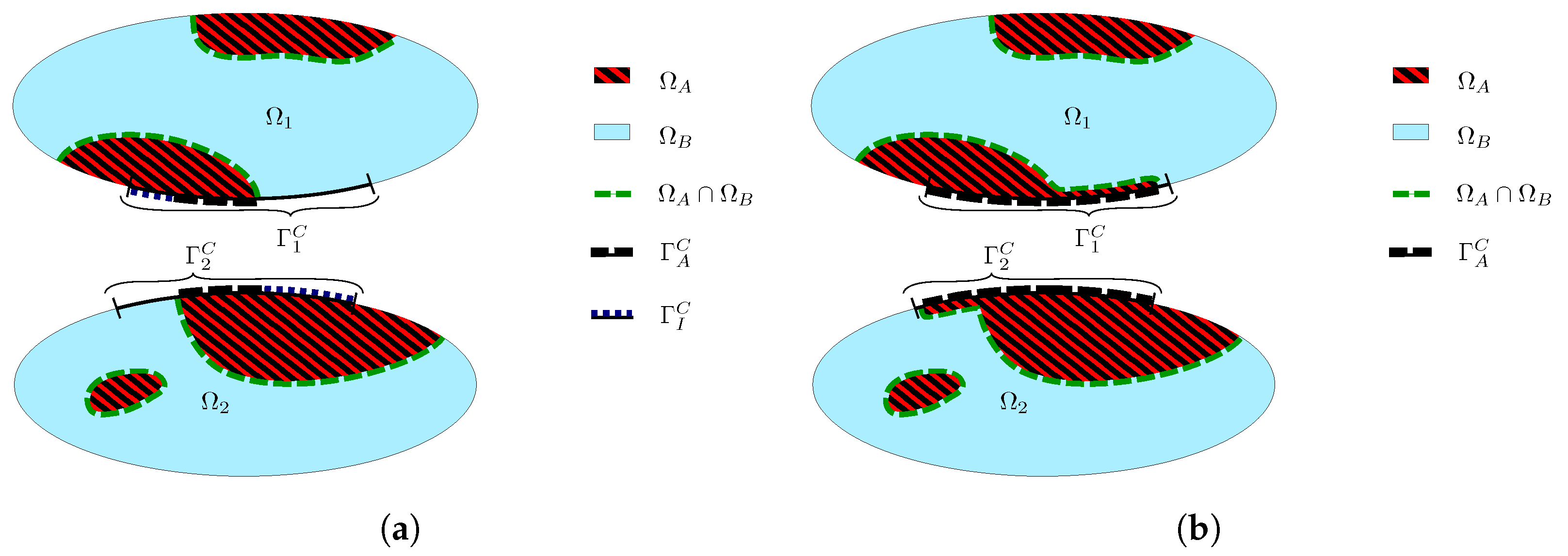
4.2. From Irregular Snapshots

The regular-based clustering strategy introduced in Section 4.1 may become prohibitive for high-dimensional parametric spaces. In such cases, an irregular distribution of snapshots in the parametric space has to be considered for the training set ${\mathcal{P}}_{tr}$, generally thanks to greedy algorithms. Then, it is no more suitable to rely on an element-wise partition of the parametric space for the clustering. A simple adaptation of the procedure of Section 4.1 is proposed here. The dissimilarity matrix is now based on the Grassmann distance between each normalized snapshot ${\underset{¯}{S}}_j$, $j=1,\dots ,M_s$, with $M_s=card\left({\mathcal{P}}_{tr}\right)$ the number of snapshots. In this case, Equation (14) reduces to

$$d_{Gr(\infty ,\infty )}({\underset{¯}{S}}_{j_1},{\underset{¯}{S}}_{j_2})=\arccos \left({\underset{¯}{S}}_{j_1}^T{\underset{¯}{S}}_{j_2}\right),\forall j_1,j_2\in {\left[[0,M_s]\right]}^2.$$

(16)

The clustering strategy returns in this case in labeling the snapshots.

Local ROMs are built similarly to Section 4.1 from the cluster-based local snapshots matrix.

The simplification of the clustering phase comes with adding complexity in the classification construction required for the online local ROM selection. Advanced classifiers, see for example [18], have to be considered as no clustering partition of the parametric space is available. In this work, we propose to build offline a supervised learning classification method trained on the snapshots and their cluster label. In the numerical examples, the random forest classification method [32,33] has been performed.

5. Numerical Results

In all of the following numerical experiments, the FOM solution was obtained thanks to the Cast3M finite elements software (2020 version) [34]. Lagrange P1 or Q1 finite elements have been used, with three or four integration points, respectively, for strain/stress calculation.

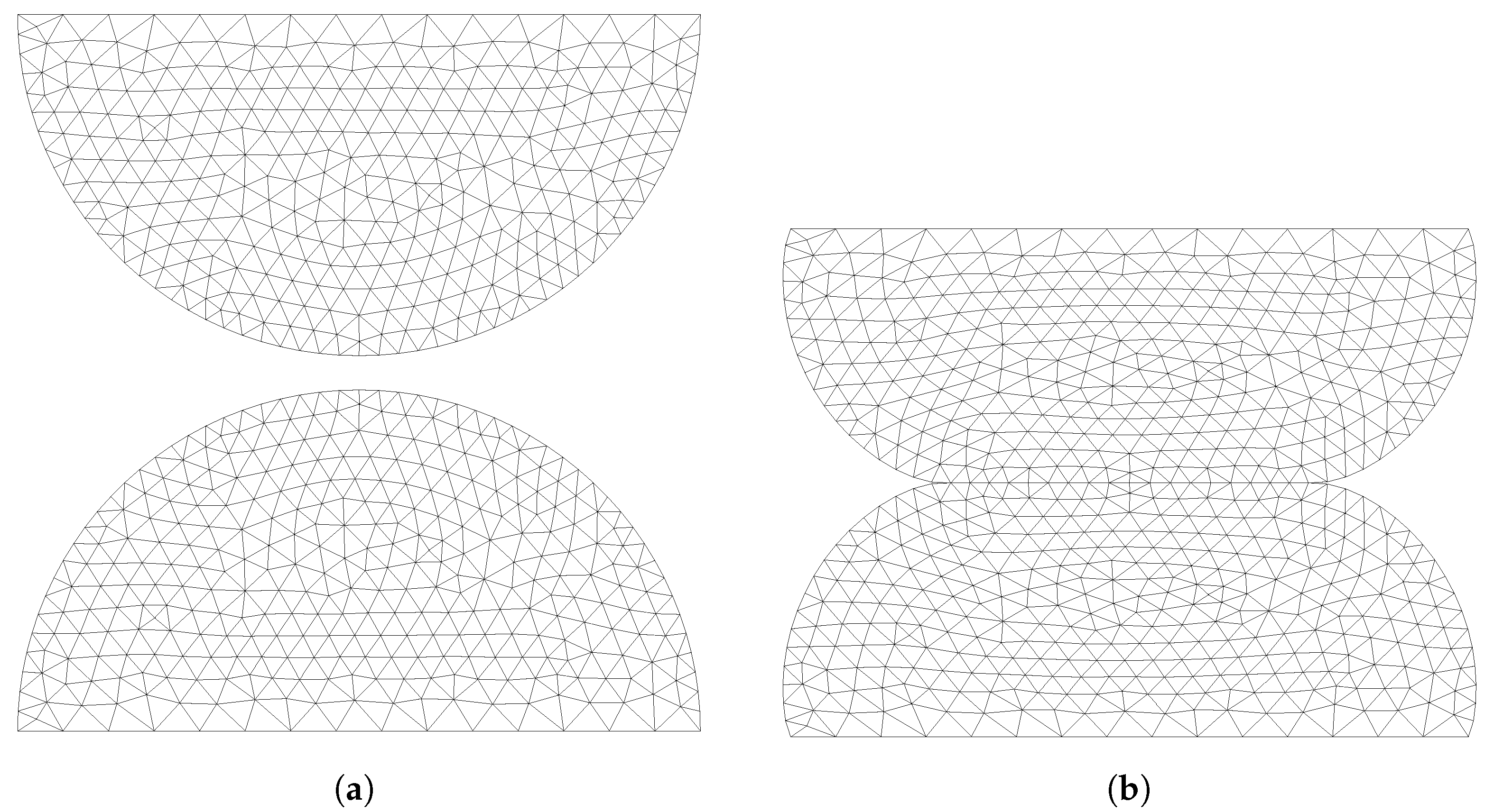
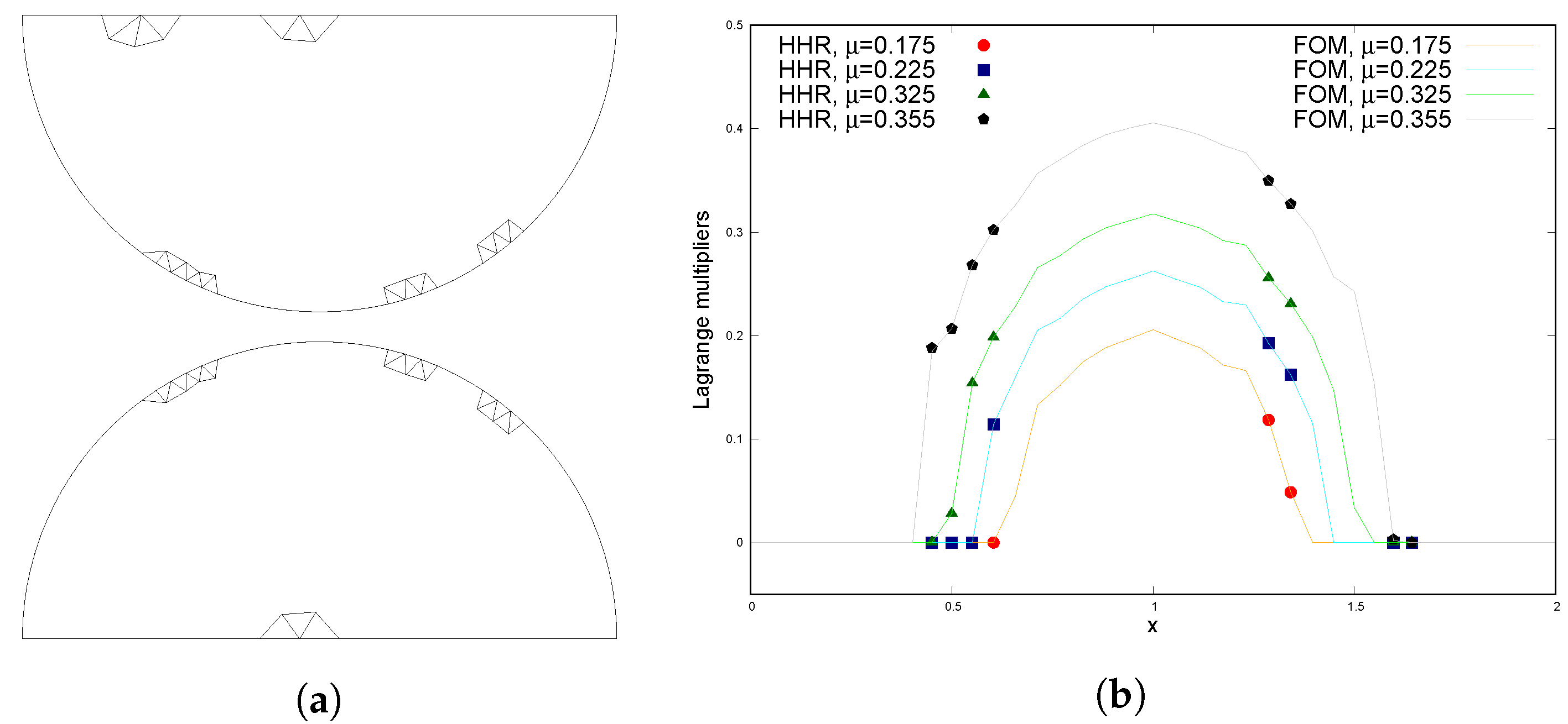
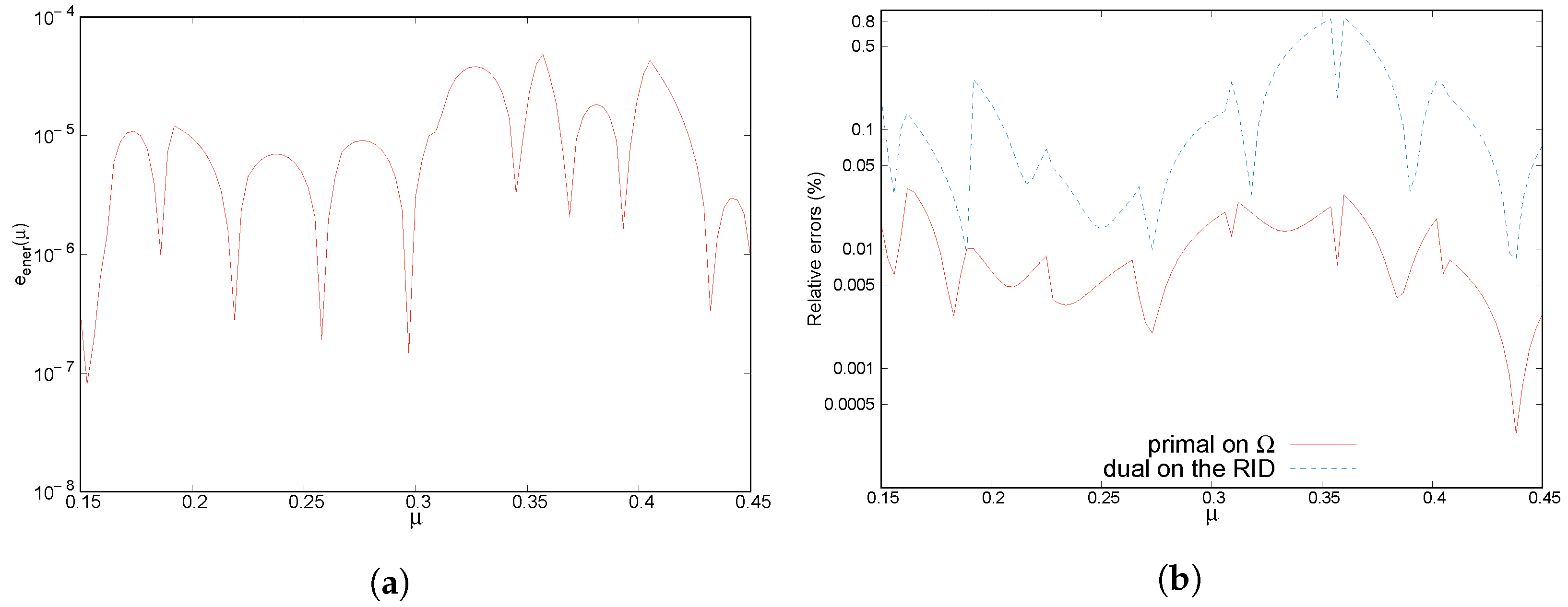
5.1. Test Case A: Half Disks of Hertz, Unidimensional Parametric Space

This test case is described in [10]. It considers two half disks in a two-dimensional setting, each disk having the same radii $R=1$ m. The two disks are separated by an initial gap being at minimum $d=0.1$ m. Both disks have the same material characteristics: a Young modulus $E=15$ Pa and a Poisson coefficient $\nu =0.35$. Dirichlet boundary conditions are imposed on the horizontal edges of the disks, with $u_x=0$ and $u_y=\pm \mu$ with an upward movement for the lower disk and a downward movement for the upper disk. The range values of $\mu$ defines the parametric space. A representation of the initial state of the test case can be seen in Figure 5a.

The finite element full-order model (FOM) is built on a mesh with 678 nodes. The circular parts of both disks, constituting the potential contact zone, contains 55 nodes on each side. The deformation obtained with the FOM for $\mu =0.3$ is presented in Figure 5b.

We consider a parametric space $\mathcal{P}=[0.15,0.45]$ (m) for $\mu$ and build the training set ${\mathcal{P}}_{tr}=\{0.15+0.01i|0\le i\le 30\}$ (m). Hence card(${\mathcal{P}}_{tr}$) = 31. To assess the accuracy of the methods on this test case, we will use three kind of errors, the primal relative error in the 2-norm Equation (17), the dual relative error in the 2-norm Equation (18), and the error on the minimum energy Equation (19) used in [10].

$$e_u\left(\mu \right)={\left(\frac{\left|\right|{\underset{¯}{u}}_{ROM}\left(\mu \right)-{\underset{¯}{u}}_{FOM}\left(\mu \right){\left|\right|}_{2,\Omega }^2}{\left|\right|{\underset{¯}{u}}_{FOM}\left(\mu \right){\left|\right|}_{2,\Omega }^2}\right)}^{\frac{1}{2}},$$

(17)

$$e_{\lambda }\left(\mu \right)={\left(\frac{\left|\right|{\underset{¯}{\lambda }}_{ROM}\left(\mu \right)-{\underset{¯}{\lambda }}_{FOM}\left(\mu \right){\left|\right|}_{2,{\Gamma }_A^C}^2}{\left|\right|{\underset{¯}{\lambda }}_{FOM}\left(\mu \right){\left|\right|}_{2,{\Gamma }_A^C}^2}\right)}^{\frac{1}{2}},$$

(18)

$$e_{ener}\left(\mu \right)=\frac{1}{2}\left|a({\underset{¯}{u}}_{ROM}\left(\mu \right),{\underset{¯}{u}}_{ROM}\left(\mu \right))-f\left({\underset{¯}{u}}_{ROM}\left(\mu \right)\right)-a({\underset{¯}{u}}_{FOM}\left(\mu \right),{\underset{¯}{u}}_{FOM}\left(\mu \right))+f\left({\underset{¯}{u}}_{FOM}\left(\mu \right)\right)\right|,$$

(19)

with $({\underset{¯}{u}}_{ROM}\left(\mu \right),{\underset{¯}{\lambda }}_{ROM}\left(\mu \right))$ and $({\underset{¯}{u}}_{FOM}\left(\mu \right),{\underset{¯}{\lambda }}_{FOM}\left(\mu \right))$ denoting the ROM (here obtained with the HHR model) and FOM solutions (primal and dual), respectively.

Let us underline that, in the case of the HHR method, the error on the Lagrange multipliers (18) is naturally evaluated on the RID. The extension from ${\Gamma }_A^C$ to ${\Gamma }^C$ could however be performed through the reconstruction strategy introduced in [9]. On the counterpart, the extension to $\Omega$ of the displacement field is obvious thanks to the POD basis. Hence, the primal error will always be evaluated on the whole domain $\Omega$.

This test case has the particularity to present a double symmetry (horizontal and vertical) for the dual and the primal solutions. This symmetry added to the relatively small contact surface and the one-dimensional parametric space leads to a test case relatively easy to treat for ROMs. Using the HHR, a small RID is enough to give very good results.

In the following results, the RID has been built from the set $\mathcal{L}$ obtained applying the DEIM to the primal POD-reduced basis. This set is supplemented by two nodes on the top and bottom surfaces to be able to treat Dirichlet boundary conditions. As the parametric space is quite small, an accurate error threshold of ${ϵ}_{\mathcal{POD}}={10}^{-8}$ is used, resulting in a primal RB with 9 vectors ($l=9$). The RID is reported in Figure 6a. It results in 16 nodes on the contact surfaces (8 on each side), hence $N_{\lambda }^C=8$. The solvability condition (cf. Equation (11) is in this case directly respected. Moreover, the condition number is also initially very good $\kappa \left(\underset{\underset{¯}{¯}}{B}[{\mathcal{A}}_{\lambda },{\mathcal{A}}_c]\underset{\underset{¯}{¯}}{V}[{\mathcal{A}}_c,:]\right)=3.4$. Hence, this test case does not require any enrichment of the primal RB to obtain accurate results with the HHR method. In Figure 6b, the Lagrange multipliers for the FE and HHR models are reported for different values of $\mu \notin {\mathcal{P}}_{tr}$. This Figure confirms the very good local accuracy on the Lagrange multipliers.

To further evaluate the accuracy the method we compute the errors $e_u\left(\mu \right)$, $e_{\lambda }\left(\mu \right)$ and $e_{ener}\left(\mu \right)$, either on the RID and on $\Omega$ (with the reconstructed dual solution) on a set of 101 points in $\mathcal{P}$ (including the 11 points of the training set ${\mathcal{P}}_{tr}$). The results are reported in Figure 7.

The primal solution is always approximated with accuracy, with relative errors in the 2-norm below 0.05% (5×10${}^{-4}$) on the parametric space. The dual solution is also approximated accurately ranging from 0.1% to a maximum of 0.8%. The error on the minimum energy is also very satisfying, with errors below ${10}^{-4}$ on $\Omega$, even outside the training set.

In [10], the cone-projected greedy (CPG) algorithm was applied on the same problem with the same training set and the same POD truncation ($l=9$ POD modes). The CPG method yields to errors ranging from ${10}^{-6}$ to ${10}^{-3}$ for the error on the minimum energy, and from ${10}^{-5}$ to 4×10${}^{-3}$ for the error on the displacement field. Those errors were obtained on parametric points of the training set only. No errors on Lagrange multipliers were reported. Compared with the errors shown in Figure 7 of the present paper, it highlights the robustness of the proposed HHR method—that is to say the accuracy of the results on the parametric space, even outside the training set.

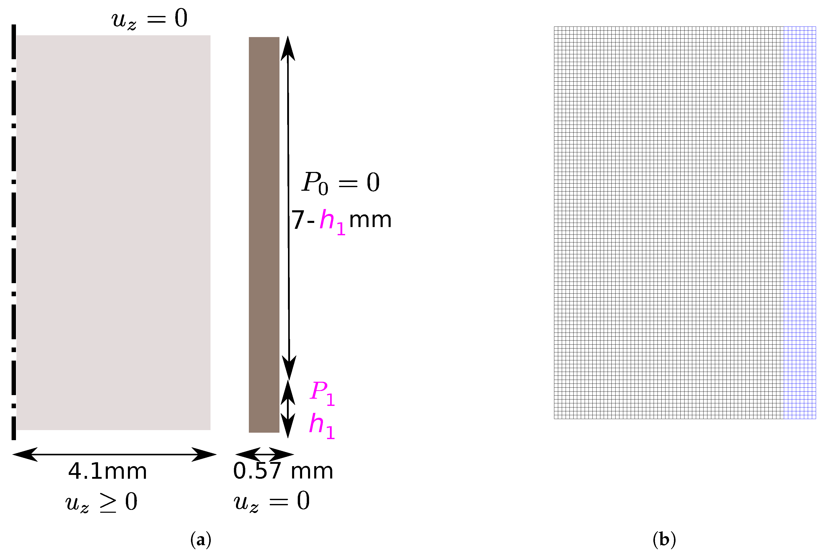
5.2. Test Case B: 2D Axisymmetric Contact—Bidimensional Parametric Space

We consider here a two-dimensional axisymmetric test case introduced in [35], representing a simplified contact problem between a nuclear fuel pellet and its surrounding cladding. The test’s geometry is sketched in Figure 8a. The two materials follow an elastic isotropic behaviour with a Young modulus and Poisson coefficient of $E=190$ GPa, $\nu =0.3$ for the fuel, and $E=78$ GPa, $\nu =0.34$ for the cladding. The uniform initial gap between the two solids is $d=2$ $\mathsf{\mu }$m. The test case consists in applying a pressure $P_1$ on a length $h_1$ on the outside part of the cladding. The range values of parameters $P_1$ and $h_1$ form the parametric space $\mathcal{P}=[5,200]$ MPa $\times [0.6,6.0]$ mm. This configuration leads to a low displacement along the z axis, allowing good modeling of the contact with a node-to-node configuration. The parametric variations are challenging for ROM models as it includes strong variations of the contact surface as well as the contact pressure. The FOM is built on a mesh with 7070 nodes, 6161 for the mesh representing the fuel and 909 for the cladding, see Figure 8b. There are 101 potential contacts ($N_{\lambda }=101$).

In order to build the HHR model, 500 snapshots regularly distributed in the parametric space are used for the training set ${\mathcal{P}}_{tr}$. Due to the large variations of the parametric space, a POD threshold of ${ϵ}_{\mathcal{POD}}={10}^{-6}$ is used to initially limit the dimension of the primal RB to $l=36$ (see the decrease of approximation error on the snapshot matrix in Section 5.2.2). Using the set of points $\mathcal{L}$ obtained from the DEIM applied to the primal RB results in the RID illustrated in Figure 9a where a region of interest corresponding to the Neumann surface has been added. The number of potential contact is the RID is $N_{\lambda }^C=12$. This RID gives ride to unsatisfactory primal solutions. We then expand the set $\mathcal{L}$ using a second DEIM on a dual POD RB (with a threshold $ϵ=4\times {10}^{-4}$). It worth underlying that this dual POD RB is only used for the RID expansion. The expanded RID is presented in Figure 9b, having also the Neumann surface as a zone of interest. In this case, $N_{\lambda }^C=34$. The advantage of using the DEIM on a dual POD RB is that the selected DoFs will be located on the contact surface.

In the following, the results presented focus on the expanded RID ($l=36$, $N_{\lambda }^C=34$) and on parameters outside of the training set ${\mathcal{P}}_{tr}$. In this case, the solvability condition is not initially respected. Hence, the primal RB have to be enriched to solve the HHR problem.

5.2.1. Enrichment Strategies

We focus here on the algorithm presented in Section 3.3 for the enrichment of the primal RB with FE shape functions. Figure 10 shows the output at the different iterations of the greedy Algorithm 1. Although the solvability condition is not verified initially, a numerical solution can be obtained. However this latter exhibits high dual relative errors. Figure 10 illustrates that the strict respect of the solvability condition (indicated by the dashed red vertical lines) is not enough to obtain a satisfying accuracy on the dual solutions. With FE shape function enrichment, the solvability condition is verified for $\overline{l}=40$ (4 supplementary FE shape functions), but with a condition number of $\underset{\underset{¯}{¯}}{B}[{\mathcal{A}}_{\lambda },{\mathcal{A}}_c]\overline{\underset{\underset{¯}{¯}}{V}}[{\mathcal{A}}_c,:]$ superior to 1000, lying to dual relative errors greater than 70%. The further enrichment of the primal RB based on the improvement of this condition number enables drastically improving the dual relative errors, up to 2% for the parametric point (170 MPa, 3.2 mm) considered in Figure 10a. The dual relative error becomes significantly lower for a condition number around 10, see Figure 10b. For ${\kappa }_{max}=10$, the greedy algorithm results in card($\overline{\underset{\underset{¯}{¯}}{V}}$) = 55 and a dual relative error of 6.3%.

The enrichment strategy of the primal RB with POD and FE modes, introduced in Section 3.4, is now compared to the enrichment strategy based on FE modes only, and previously illustrated. We set ${\kappa }_{max}=1$ (maximal enrichment) in Algorithm 1 for both approaches. We report in

Table 1. The 2D axisymmetric test case: study of the enrichment strategy by POD modes and FE shape functions ($l=36$ et $N_{\lambda }^C=34$).

					${{P}}_1=170$ MPa		${\mathit{P}}_1=30$ MPa
					$h_1=3.2$ mm		$h_1=5.25$ mm
	nb POD	${ϵ}_{\mathcal{POD}2}$	$\kappa (\underset{\underset{¯}{¯}}{B}[{\mathcal{A}}_{\lambda },{\mathcal{A}}_c]$ $\overline{\underset{\underset{¯}{¯}}{V}}[{\mathcal{A}}_c,:])$	$\overline{l}=card\left(\overline{\underset{\underset{¯}{¯}}{V}}\right)$	Rel. err.		Rel. err.
	mod. add.	$\times {10}^{-7}$	after POD enrich.	Final	Primal	Dual	Primal	Dual
FE Enr.	0	−	1.5 × 10${}^6$	70	1.0%	2.5%	2.9%	21%
POD+FE Enr.	3	7.5	2.3 × 10${}^4$	73	2.5%	1.8%	0.5%	26%
POD+FE Enr.	6	5	4.5 × 10${}^3$	76	0.5%	1.6%	1.6%	16%
POD+FE Enr.	9	3.5	4.1 × 10${}^3$	79	0.1%	1.3%	3.5%	5.6%
POD+FE Enr.	12	2.7	3.4 × 10${}^3$	82	1.4%	1.7%	2.5%	6.7%
POD+FE Enr.	15	2.2	878	85	1.9%	1.7%	1.3%	5.8%
POD+FE Enr.	18	1.7	386	88	1.1%	1.4%	0.2%	5.3%
POD+FE Enr.	21	1.3	383	91	7.8%	1.8%	13.4%	9.3%
POD+FE Enr.	23	1.1	330	93	0.8%	1.3%	16%	9.9%
POD+FE Enr.	26	0.9	328	96	12%	1.3%	1.5%	9.5%

the results obtained for different truncation levels for the enrichment by POD modes on two points of the parametric space (strong or weak contact) outside the training set ${\mathcal{P}}_{tr}$.

The enrichment method by POD+FE modes can enable us to reach dual and primal relative errors lower than the enrichment method with only FE modes. Using a maximal enrichment ${\kappa }_{max}=1$, the enrichment method by extended POD naturally leads to higher cardinal of the primal extended RB (see Table 1).

Regarding the errors, we can see that for a parametric point already well treated by the FE enrichment method (see $P_1=170$ MPa and $h_1=3.2$ mm), few additional POD modes are enough to lower the dual relative error. However, when the dual relative errors remain high with the FE enrichment method, it is useful to add more POD modes to lower the dual relative error. For example, on the point $P_1=30$ MPa and $h_1=5.25$ mm, adding 9 POD modes (corresponding to ${ϵ}_{\mathcal{POD}2}$ = 3.5 ×${10}^{-7}$) allows us to divide the dual relative error by four.

We can outline from Table 1 that the choice of ${ϵ}_{\mathcal{POD}2}$ remains non-trivial as (too) low values lead to phenomena associated with over-fitting that degrade the accuracy of the solutions.

We notice that an enrichment method with POD modes only will not be efficient to lower the condition number of the projected contact rigidity matrix without impacting the precision of the reduced solutions.

In Figure 10, the output of the greedy algorithm on the primal RB extended with nine supplementary POD modes (denoted as ‘l + 9’ in the legend) are reported. For an equivalent primal RB dimension, the POD+EF enrichment strategy becomes interesting only for low errors, see Figure 10a. However regarding to condition number of the projected contact rigidity matrix, the POD+FE enrichment strategy is always improving the dual errors for a given prescribed condition number, see Figure 10b. It is worth noting that the solvability condition is reached for a comparable condition number. This confirms the strong relation between solvability, precision, and condition number.

The two enrichment methods are now compared on the whole parametric space. For that purpose, HHR solutions are calculated on 6400 points regularly distributed in the parametric space. We set the maximum condition number to ${\kappa }_{max}=10$, which seems to be a good compromise between precision and dimension of the extended primal RB.

The maps of the dual relative errors are reported in Figure 11 for the FE enrichment strategy (Figure 11b) and POD+EF enrichment strategy with 9 supplementary POD modes (Figure 11a). It clearly shows an improvement due to the POD+EF enrichment method. The dimension of the final extended primal RB ($\overline{l}$) is, in this case, 7 modes larger (instead of 9), which implies that the improvement of the condition number is slightly facilitated by the addition of POD modes.

Whatever the enrichment strategy, dual relative errors remain high on the left side of the maps, for low pressures $P_1$. This highlights the complexity to efficiently reduce a problem on such a parametric space, where the contact can be strong, weak, or even absent, and on a large or small surface.

This naturally opens the way to study clustering strategies on the parametric space.

Before presenting numerical results for the clustering strategies, we first study here the impact of the size of the RID over the enrichment strategies. We hence consider a larger extended RID with more potential contact points. This RID is simply obtained considering a higher dual POD RB threshold of $ϵ=1\times {10}^{-4}$ for the DEIM point selection, see Section 5.2. In this case, the RID contains $N_{\lambda }^C=60$ potential contacts with always the same primal RB of $l=36$ POD modes, see Figure 12.

As a consequence of the augmentation of $N_{\lambda }^C$, the solvability condition requires a larger enriched primal RB. For this RID, the FE enrichment method reaches the solvability condition for $\overline{l}=61$; that is to say, 35 supplementary FE modes. However, as previously shown, for this extended basis, the dual reduced solutions are not satisfying enough. Further enrichment based on the condition number of the projected contact rigidity matrix is required.

In Figure 13, we report dual relative error maps using both FE and POD+FE enrichment with a maximal condition number ${\kappa }_{max}=10$. This results in a primal RB with a cardinal of $\overline{l}=83$ for the FE enrichment method and of $\overline{l}=91$ for the POD+FE enrichment method with nine supplementary POD modes ($l+9$). Compared to Figure 11a, the first conclusion to be drawn is that the increase of $N_{\lambda }^C$ does not improve the error maps for the FE enrichment method, see Figure 13a. In counterpart, we can see a significant improvement for the POD+FE enrichment method, cf. Figure 11a and Figure 13b.

An important point here is to remember that the RID contains more Lagrange multipliers when $N_{\lambda }^C=60$ than when $N_{\lambda }^C=34$, meaning that the computation of the dual relative error as defined by (18) implies more forces in the case $N_{\lambda }^C=60$. Contact forces for the parametric point $P_1=170$ MPa and $h_1=3.2$ mm for both configuration of $N_{\lambda }^C$ with full FE enrichment (${\kappa }_{max}=1$) are reported in Figure 14. In both situations, the dual forces are locally very accurate on the RID ($2.6\%$ for $N_{\lambda }^C=60$, and $2.5\%$ for $N_{\lambda }^C=34$). However, having more potential contact points in the RID and, therefore, more contact forces solved is obviously an advantage both for the physical interpretation of the simulation and the reconstruction of the dual solution, but the drawback is the dimension of the primal RB that grows with $N_{\lambda }^C$.

This motivates one to, furthermore, look to forward clustering approaches to limit the increase of the primal RB cardinal while reaching the same accuracy.

5.2.2. Clustering Strategies

From Regular Snapshots

We focus here on the clustering strategy proposed in Section 4.1. The same regular training set ${\mathcal{P}}_{tr}$ composed by 500 snapshots is used. The partition of parametric space is built through groups of four snapshots forming rectangles in the 2D parametric space representation, see Figure 15a. In Figure 15b we can see the results of the clustering algorithm for $K=3$ clusters, each point representing a snapshot and the background color representing a cluster.

The clusters contain respectively 170, 194, and 170 snapshots in their local snapshot matrices. Figure 15b shows that the clustering strategy on the parametric space naturally focuses on the position $h_1$ of the potential contact zone. It confirms that a large variation of the potential contact zone is the preponderant parameter of nonlinearity.

As the parametric space is locally reduced into the cluster, the local HHR models are obtained from a primal POD threshold ${ϵ}_{\mathcal{POD}}={10}^{-8}$. The choice of this threshold still enables a low-rank approximation as confirmed by Figure 16.

The primal RB size in each cluster is $l=\{31,39,36\}$. A local RID is built for each local model. As previously, a DEIM on the primal RB and a contribution from a DEIM on a dual POD RB (with a threshold $ϵ={10}^{-6}$) is used to obtain the set of nodes $\mathcal{L}$. The resulting RIDs are reported in Figure 17. The number of potential contacts treated in each RID is $N_{\lambda }^C=\{36,40,35\}$.

As a direct results of the cluster shapes, the RID of the local reduced order models are much more localized. Figure 17 confirms the observation made from Figure 15b, as the three RIDs finally form a domain decomposition of the FOM potential contact zone. For each cluster, the RID is localized around the possible values of $h_1$, which represents the zone of status change (contact/gap).

On each cluster, the primal RB extension is performed through the FE enrichment strategy only (since ${ϵ}_{\mathcal{POD}}$ is already low). The results obtained with a maximum enrichment (${\kappa }_{max}=1$) for the two points studied in Table 1 are reported in

Table 2. 2D axisymmetric test case. Study of the clustering strategy with full local FE enrichment.

	Cluster	$\mathit{\kappa }(\underset{\underset{¯}{¯}}{\mathit{B}}[{\mathcal{A}}_{\mathit{\lambda }},{\mathcal{A}}_{\mathit{c}}]$ $\overline{\underset{\underset{¯}{¯}}{\mathit{V}}}[{\mathcal{A}}_{\mathit{c}},:])$	$\mathit{l}=card\left(\underset{\underset{¯}{¯}}{\mathit{V}}\right)$	$\overline{\mathit{l}}=card\left(\overline{\underset{\underset{¯}{¯}}{\mathit{V}}}\right)$	Rel. err.
	Label	before FE enrich.	Initial	Final	Primal	Dual
$P_1=170$ MPa $h_1=3.2$ mm	2	1.5 × 10${}^5$	39	79	0.03%	2.0%
$P_1=30$ MPa $h_1=5.25$ mm	1	2.2 × 10${}^4$	31	67	0.02%	2.4%

.

For the point $P1=170$ MPa and $h_1=3.2$ mm, already accurately treated by the enrichment strategies performed on the whole parametric space, similar dual errors are obtained (with a significant improvement on the primal error).

For the point $P1=30$ MPa and $h_1=5.25$ mm, the results are much better than the ones obtained on the whole parametric space, whatever the enrichment strategy (see Table 1). Moreover, the size of the primal RB remains limited ($\overline{l}=67$).

Generally speaking, the proposed clustering strategy helps smooth the dual relative errors. It particularly improves the accuracy on the parametric points where the relative errors are high without the clustering strategy, see Figure 18.

Concerning the RB dimensions, this clustering strategy leads to comparable sizes than the strategies introduced in Section 5.2.1 However the dual errors are greatly improved by the clustering compared to Figure 11.

The error maps of Figure 18 are even better than the ones obtained on an extended RID with the POD+EF enrichment strategy, see Figure 13b. In this latter case, the bases dimensions were almost $40\%$ larger.

We should note that, even with the clustering strategy, it remains difficult to accurately approximate very low contact pressure parametric zones.

The number of clusters K cannot be too increased. Indeed, the more the cluster, the smaller the local parametric space becomes. However, each cluster must have enough snapshots to build a representative POD RB and then an accurate HHR model.

More snapshots could be initially used, but another interesting way to investigate would be to consider a recursive clustering strategy (with possibly adding snapshots) inside clusters having the least accurate HHR solutions.

From Irregular Snapshots

We focus here on an irregular distribution of the snapshots in the parametric space $\mathcal{P}$ obtained through a snapshot selection by the greedy algorithm introduced in [9]. The resulting training set ${\mathcal{P}}_{tr}$ contains 200 snapshots, which can be visualized in Figure 19a. Let us notice that they are mainly located around small values of contact pressure $P_1$.

In order to appreciate the solutions obtained by the clustering algorithm introduced in Section 4.2, we first briefly present some key results obtained by the HHR method with enrichment trained on irregular snapshots of ${\mathcal{P}}_{tr}$ (without clustering).

The HHR model is built using the primal POD threshold ${ϵ}_{\mathcal{POD}}={10}^{-6}$, resulting in a primal RB of dimension $l=33$. The RID is obtained as the one shown in Figure 12 (DEIM on the primal RB, and a contribution from a DEIM on a POD dual RB obtained with the threshold $ϵ={10}^{-4}$). It finally contains $N_{\lambda }^C=57$ potential contacts. For the POD+FE enrichment method, an error threshold ${ϵ}_{\mathcal{POD}2}=3.5\times {10}^{-7}$ is used (as in Figure 11b and Figure 13b) resulting in a primal RB of dimension $(l+5)=38$ before enrichment. Both enrichment strategies are moreover applied, setting ${\kappa }_{max}=10$ as a maximum condition number in Algorithm 1. The FE enrichment method results in a primal RB of cardinal $\overline{l}=60$, while the POD+FE method results in a primal RB of cardinal $\overline{l}=82$. We present in Figure 20 the dual relative errors on the parametric space for both reduced models.

The errors are in good agreement with those obtained with 500 regular snapshots on a RID of similar size, see Figure 13. It is worth noting that better results are globally reached (especially for low contact pressure) and with a more compact primal RB (lower dimension). This confirms the interest of greedy-selected snapshots [9].

In order to evaluate the clustering strategy based on irregular snapshots (cf. Section 4.2) on this training set, we build $K=3$ clusters through the k-medoid algorithm (as for the previous clustering strategy based on regular snapshots). In Figure 19a, the cluster labels are reported. The random forest classifier is then trained to obtain a prediction function, represented in Figure 19b as a partition of the parametric space. Let us note that, in this case, the clusters are not uniquely defined thanks to the contact position $h_1$ but also according to the pressure values $P_1$ for small $h_1$. It confirms that a small contact pressure applied to a reduced contact area is difficult to capture.

The local reduced order models are built with the same strategy than for the clustering on regular snapshots. The associated local RIDs are shown in Figure 21. As for the regular snapshot case, the RIDs are localized around the potential contact surface of the cluster ($h_1$ parameter). RIDs of cluster 0 and 2 are quite similar.

The dual errors map is shown in Figure 22. The clustering strategy helps smooth the dual relative errors, as observed previously. The errors are considerably reduced for RB of comparable sizes to those without clustering (cf. Figure 20), even for low contact pressures.

As an improvement, we can see that an adaptive snapshots strategy into clusters could be interesting since big clusters (see cluster 1) may lack snapshots and since the cluster delimitation could be improved where snapshots are sparsely distributed.

6. Conclusions

Efficient strategies to improve the dual solution precision of reduced order modeling of contact mechanics problems treated by Lagrange multipliers have been proposed. We focused on the hybrid hyper-reduced (HHR) method where the dual reduced basis returns to a restriction on a reduced integration domain of the full order dual basis.

First, the strong correlation between the condition number of the projected contact rigidity matrix and the accuracy of the dual solution was highlighted. Two strategies of enrichment of the primal POD reduced basis were introduced. These strategies allowed us to verify the solvability condition of the reduced saddle-point problem (if not respected initially) and improve the accuracy of the method, especially the dual solution.

Secondly, for a large parametric space, especially for large variations of the contact zone where the non-smoothness of the contact conditions makes difficult low rank dual approximations, clustering-based strategies have been proposed. Precise local enriched HHR models are then built leading to globally enhance the accuracy of the reduced model using limited sizes of reduced bases. Clustering strategies have been presented for regular or irregular snapshots.

These different strategies have been applied on two-dimensional test cases, demonstrating very good accuracy of the method on small parametric spaces, and the usefulness contribution of the enrichment and clustering strategies on large parametric spaces. The HHR method is able to accurately treat non-smooth cases where the contact forces can be strong or weak, and very localized or extended.

Future works will focus on the extension of the HHR to more complex geometries where node-to-segment contact detection is required.

References

1. Balajewicz, M.; Toivanen, J. Reduced order models for pricing European and American options under stochastic volatility and jump-diffusion models. J. Comput. Sci. 2017, 20, 198–204. [Google Scholar] [CrossRef]
2. Bader, E.; Zhang, Z.; Veroy, K. An empirical interpolation approach to reduced basis approximations for variational inequalities. Math. Comput. Model. Dyn. Syst. 2016, 22, 345–361. [Google Scholar] [CrossRef]
3. Scheffold, D.; Bach, C.; Duddeck, F.; Müller, G.; Buchschmid, M. Vibration Frequency Optimization of Jointed Structures with Contact Nonlinearities using Hyper-Reduction. IFAC-PapersOnLine 2018, 51, 843–848. [Google Scholar] [CrossRef]
4. Ballani, J.; Huynh, D.B.P.; Knezevic, D.J.; Nguyen, L.; Patera, A.T. A component-based hybrid reduced basis/finite element method for solid mechanics with local nonlinearities. Comput. Methods Appl. Mech. Eng. 2018, 329, 498–531. [Google Scholar] [CrossRef]
5. Giacoma, A.; Dureisseix, D.; Gravouil, A.; Rochette, M. A multiscale large time increment/FAS algorithm with time-space model reduction for frictional contact problems. Int. J. Numer. Methods Eng. 2014, 97, 207–230. [Google Scholar] [CrossRef] [Green Version]
6. Giacoma, A.; Dureisseix, D.; Gravouil, A. An efficient quasi-optimal space-time PGD. Application to frictional contact mechanics. Adv. Model. Simul. Eng. Sci. 2016, 3, 1–17. [Google Scholar] [CrossRef] [Green Version]
7. Haasdonk, B.; Wohlmuth, B.; Salomon, J. A Reduced Basis Method for Parametrized Variational Inequalities. SIAM J. Numer. Anal. 2012, 50, 2656–2676. [Google Scholar] [CrossRef] [Green Version]
8. Balajewicz, M.; Amsallem, D.; Farhat, C. Projection-based model reduction for contact problems. Int. J. Numer. Methods Eng. 2016, 106, 644–663. [Google Scholar] [CrossRef] [Green Version]
9. Fauque, J.; Ramière, I.; Ryckelynck, D. Hybrid hyper-reduced modeling for contact mechanics problems. Int. J. Numer. Methods Eng. 2018, 115, 117–139. [Google Scholar] [CrossRef]
10. Benaceur, A.; Ern, A.; Ehrlacher, V. A reduced basis method for parametrized variational inequalities applied to contact mechanics. Int. J. Numer. Methods Eng. 2019, 121, 1170–1197. [Google Scholar] [CrossRef]
11. Barrault, M.; Maday, Y.; Nguyen, N.C.; Patera, A.T. An ‘empirical interpolation’ method: Application to efficient reduced-basis discretization of partial differential equations. Comptes Rendus Math. 2004, 339, 667–672. [Google Scholar] [CrossRef]
12. Chaturantabut, S.; Sorensen, D.C. Nonlinear Model Reduction via Discrete Empirical Interpolation. SIAM J. Sci. Comput. 2010, 32, 2737–2764. [Google Scholar] [CrossRef]
13. Astrid, P.; Weiland, S.; Willcox, K.; Backx, T. Missing Point Estimation in Models Described by Proper Orthogonal Decomposition. IEEE Trans. Autom. Control 2008, 53, 2237–2251. [Google Scholar] [CrossRef] [Green Version]
14. Farhat, C.; Avery, P.; Chapman, T.; Cortial, J. Dimensional reduction of nonlinear finite element dynamic models with finite rotations and energy-based mesh sampling and weighting for computational efficiency. Int. J. Numer. Methods Eng. 2014, 98, 625–662. [Google Scholar] [CrossRef]
15. Ryckelynck, D. Hyper-reduction of mechanical models involving internal variables. Int. J. Numer. Methods Eng. 2009, 77, 75–89. [Google Scholar] [CrossRef]
16. Delhez, E.; Nyssen, F.; Golinval, J.C.; Batailly, A. Reduced order modeling of blades with geometric nonlinearities and contact interactions. J. Sound Vib. 2021, 500, 116037. [Google Scholar] [CrossRef]
17. Manvelyan, D.; Simeon, B.; Wever, U. An efficient model order reduction scheme for dynamic contact in linear elasticity. Comput. Mech. 2021, 68, 1283–1295. [Google Scholar] [CrossRef]
18. Daniel, T.; Casenave, F.; Akkari, N.; Ryckelynck, D. Model order reduction assisted by deep neural networks (ROM-net). Adv. Model. Simul. Eng. Sci. 2020, 7, 16. [Google Scholar] [CrossRef]
19. Amsallem, D.; Zahr, M.; Washabaugh, K. Fast local reduced basis updates for the efficient reduction of nonlinear systems with hyper-reduction. Adv. Comput. Math. 2015, 41, 1187–1230. [Google Scholar] [CrossRef]
20. Redeker, M.; Haasdonk, B. A POD-EIM reduced two-scale model for crystal growth. Adv. Comput. Math. 2015, 41, 987–1013. [Google Scholar] [CrossRef]
21. Peherstorfer, B.; Butnaru, D.; Willcox, K.; Bungartz, H.J. Localized Discrete Empirical Interpolation Method. SIAM J. Sci. Comput. 2014, 36, A168–A192. [Google Scholar] [CrossRef]
22. Grimberg, S.; Farhat, C.; Tezaur, R.; Bou-Mosleh, C. Mesh sampling and weighting for the hyperreduction of nonlinear Petrov–Galerkin reduced-order models with local reduced-order bases. Int. J. Numer. Methods Eng. 2021, 122, 1846–1874. [Google Scholar] [CrossRef]
23. Duvaut, G.; Lions, J.L. Inequalities in Mechanics and Physics; Springer Science & Business Media: Berlin, Germany, 1976. [Google Scholar] [CrossRef]
24. Kikuchi, N.; Oden, J. Contact Problems in Elasticity: A Study of Variational Inequalities and Finite Element Methods; Society for Industrial and Applied Mathematics: Philadelphia, PA, USA, 1987. [Google Scholar]
25. Wriggers, P. Computational Contact Mechanics; Springer Science: Berlin, Germany, 2006. [Google Scholar] [CrossRef]
26. Babuška, I. The Finite Element Method with Lagrangian Multipliers. Numer. Math. 1973, 20, 179–192. [Google Scholar] [CrossRef]
27. Brezzi, F. On the existence, uniqueness and approximation of saddle-point problems arising from Lagrangian multipliers. In ESAIM: Mathematical Modelling and Numerical Analysis—Modélisation Mathématique et Analyse Numérique; Cambridge University Press: Cambridge, UK, 1974; Volume 8, pp. 129–151. [Google Scholar] [CrossRef]
28. El-Abbasi, N.; Bathe, K.J. Stability and patch test performance of contact discretizations and a new solution algorithm. Comput. Struct. 2001, 79, 1473–1486. [Google Scholar] [CrossRef] [Green Version]
29. Sirovich, S. Turbulence and the dynamics of coherent structures. Parts I–III. Quart. Appl Math. 1987, 45, 561–590. [Google Scholar] [CrossRef] [Green Version]
30. Ryckelynck, D.; Goessel, T.; Nguyen, F. Mechanical dissimilarity of defects in welded joints via Grassmann manifold and machine learning. Comptes Rendus. Mécanique 2020, 348, 911–935. [Google Scholar] [CrossRef]
31. Park, H.; Jun, C. A simple and fast algorithm for K-medoids clustering. Expert Syst. Appl. 2009, 36, 3336–3341. [Google Scholar] [CrossRef]
32. Breiman, L. Random Forests. Mach. Learn. 2001, 45. [Google Scholar] [CrossRef] [Green Version]
33. Pedregosa, F.; Varoquaux, G.; Gramfort, A.; Michel, V.; Thirion, B.; Grisel, O.; Blondel, M.; Prettenhofer, P.; Weiss, R.; Dubourg, V.; et al. Scikit-learn: Machine Learning in Python. J. Mach. Learn. Res. 2011, 12, 2825–2830. [Google Scholar]
34. Cast3M. Available online: http://www-cast3m.cea.fr (accessed on 16 January 2022).
35. Liu, H.; Ramière, I.; Lebon, F. On the coupling of local multilevel mesh refinement and ZZ methods for unilateral frictional contact problems in elastostatics. Comput. Methods Appl. Mech. Eng. 2017, 323, 1–26. [Google Scholar] [CrossRef] [Green Version]
Figure 1. Contact model problem.
Mathematics 10 01495 g001
Figure 2. Modification of the RID definition for the contact problems. (a) Extended RID interface ( Γ I C ). (b) Extended RID ( Ω A ).
Mathematics 10 01495 g002
Figure 3. Impact of the condition number of the projected contact rigidity matrix on the dual and primal relative errors.
Mathematics 10 01495 g003
Figure 4. Clustering framework.
Mathematics 10 01495 g004
Figure 5. Half-disk test case. FOM configurations. (a) Initial state. (b) Deformation for μ = 0.3 .
Mathematics 10 01495 g005
Figure 6. Half-disks test case. HHR model: RID and Lagrange multipliers. l = 9 , N λ C = 8 . (a) Reduced integration domain (RID). (b) Lagrange multipliers for different values of μ P t r .
Mathematics 10 01495 g006
Figure 7. Half-disks test case. HHR errors evaluations of 101 points. l = 9 , N λ C = 8 . (a) Error on the minimum energy e e n e r ( μ ) . (b) Primal error on the displacement field e u ( μ ) on Ω and dual error of the Lagrange multipliers e λ ( μ ) on the RID.
Mathematics 10 01495 g007
Figure 8. The 2D axisymmetric test case. Sketch of the problem and FOM discretization. (a) Geometry of the 2D axisymmetric test case. (b) FOM mesh.
Mathematics 10 01495 g008
Figure 9. The 2D axisymmetric test case. Reduced integration domain (RID). (a) RID obtained with one DEIM. ( l = 36 , N λ C = 12 ). (b) RID obtained with two DEIM. ( l = 36 , N λ C = 34 ).
Mathematics 10 01495 g009
Figure 10. The 2D axisymmetric test case. Study of the two enrichment strategies: by FE modes only (‘l’) and by POD+FE (‘l + 9’, 9 POD modes added), with l = 36 and N λ C = 34 . Point: P 1 = 170 MPa and h 1 = 3.2 mm. (a) Dual relative error regarding the number of FE modes added to the primal POD RB enriched (‘l + 9’) or not (‘l’). (b) Relative dual errors regarding the condition number of the projected contact rigidity matrix for the two enrichment strategies.
Mathematics 10 01495 g010
Figure 11. The 2D axisymmetric test case. Dual relative error maps (in %) for the HHR model with l = 36 , N λ C = 34 on a test space of 6400 points. Enrichment strategies applied with κ m a x = 10 . (a) FE enrichment. l ¯ = 55 . (b) POD+FE enrichment (l + 9). l ¯ = 62 .
Mathematics 10 01495 g011
Figure 12. The 2D axisymmetric test case. Larger extended RID. l = 36 , N λ C = 60 .
Mathematics 10 01495 g012
Figure 13. The 2D axisymmetric test case. Dual relative error maps (in %) for the HHR model with l = 36 , N λ C = 60 on a test space of 6400 points. Enrichment strategies applied with κ m a x = 10 . (a) FE enrichment. l ¯ = 83 . (b) POD+FE enrichment (l + 9). l ¯ = 91 .
Mathematics 10 01495 g013
Figure 14. The 2D axisymmetric test case. Contact forces for P 1 = 170 MPa and h 1 = 3.2 mm. HHR with FE enrichment (red arrows) and FOM (black arrows). (forces superposed on the right side). (a) HHR with l = 36 , N λ C = 34 and l ¯ = 70 . (b) HHR with l = 36 , N λ C = 60 and l ¯ = 96 .
Mathematics 10 01495 g014
Figure 15. The 2D axisymmetric test case. Partition and clustering of the parametric space from regular snapshots. (a) Partition of the parametric space. (b) Clusters for K = 3 .
Mathematics 10 01495 g015
Figure 16. The 2D axisymmetric test case. Approximation error (definition recalled in Appendix A) on the snapshot matrices for the case with (K = 3) and without clustering.
Mathematics 10 01495 g016
Figure 17. The 2D axisymmetric test case. (a) RID for the ROM associated with cluster 1. ( l = 31 , N λ C = 36 ). (b) RID for the ROM associated with cluster 2. ( l = 39 , N λ C = 40 ). (c) RID for the ROM associated with cluster 3. ( l = 36 , N λ C = 35 ).
Mathematics 10 01495 g017
Figure 18. The 2D axisymmetric test case. Dual relative error map (in %) for the clustering strategy with K = 3 clusters. Test space of 6400 points. FE enrichment method with κ m a x = 10 . HHR models with l = { 31 , 39 , 36 } , N λ C = { 36 , 40 , 35 } and l ¯ = { 54 , 67 , 57 } .
Mathematics 10 01495 g018
Figure 19. The 2D axisymmetric test case. Clustering strategy for irregular snapshots. K = 3 clusters. (a) Cluster labels on the irregular snapshots. (b) Prediction function obtained with the random forest classifier. (label 0: blue, label 1: grey, label 2: red).
Mathematics 10 01495 g019
Figure 20. The 2D axisymmetric test case. Irregular snapshots in the training set. Dual relative error maps (in %) for the HHR model with l = 33 , N λ C = 57 on a test space of 6400 points. Enrichment strategies applied with κ m a x = 10 . (a) FE enrichment. l ¯ = 60 . (b) POD + FE enrichment (l + 5). l ¯ = 82 .
Mathematics 10 01495 g020
Figure 21. The 2D axisymmetric test case. Irregular snapshots. RIDs associated to the local ROMs. (a) Cluster 0. ( l = 27 , N λ C = 36 ). (b) Cluster 1. ( l = 35 , N λ C = 56 ). (c) Cluster 2. ( l = 23 , N λ C = 35 ).
Mathematics 10 01495 g021
Figure 22. The 2D axisymmetric test case. Irregular snapshots. Dual relative errors map (in %) for the clustering strategy with K = 3 clusters. FE enrichment method with κ m a x = 10 . HHR models with l = { 27 , 35 , 23 } , N λ C = { 36 , 56 , 35 } and l ¯ = { 52 , 77 , 48 } .
Mathematics 10 01495 g022