Robust Nonsmooth Interval-Valued Optimization Problems Involving Uncertainty Constraints

Abstract

In this paper, Karush-Kuhn-Tucker type robust necessary optimality conditions for a robust nonsmooth interval-valued optimization problem (UCIVOP) are formulated using the concept of LU-optimal solution and the generalized robust Slater constraint qualification (GRSCQ). These Karush-Kuhn-Tucker type robust necessary conditions are shown to be sufficient optimality conditions under generalized convexity. The Wolfe and Mond-Weir type robust dual problems are formulated over cones using generalized convexity assumptions, and usual duality results are established. The presented results are illustrated by non-trivial examples.

1. Introduction

Robust optimization has become a prominent predetermined framework for investigating multi-objective optimization problems with data uncertainty. Robust optimization is a relatively new field of research that allows academicians to solve a wide range of optimization problems, particularly when challenged with real-life situations where the data input for a multi-objective linear semi-infinite program is frequently noisy or uncertain due to prediction or measurement inaccuracies, as well as in industrial settings. Under this framework, the objective and constraint functions are only considered to belong to “uncertainty sets” in function space. For single-objective optimization problems, Soyster [1] was the first researcher to study robust optimization problem. Quality products are necessary in sectors as the engineering environment grows increasingly competitive. Variations in various engineering procedures generate unexpected deviations from the function that a designer intended for. The goal of robust design is to avoid such occurrences. In industrial engineering, robust design has been developed to improve product quality and reliability. “Robustness is defined as the capacity of a technology, product, or process to work with little sensitivity to elements that cause unpredictability (in the manufacturing or user environment) and ageing while maintaining the lowest unit manufacturing cost.” explained Taguchi [2], the pioneer of robust design. For more recent developments on robust optimization problems, the readers are advised to refer to [3,4,5,6,7,8]. Lee et al. [9] and Oksanen et al. [10] used robustness for transforming data to prognostic information and open platform communications technology for agricultural machinery telemetry respectively. Lie et al. [11] used robustness in electrical machines which greatly increased motor performance and diminished computational cost. Further, robust optimization has several real life applications, readers are advised to refer to [12,13,14,15].

An interval-valued optimization problem is based on interval coefficients with closed intervals. Interval-valued optimization problems can contribute a more useful alternative for evaluating the uncertainty therein. In recent years, interval-valued optimization has become a major topic in applied mathematics. This is due to the fact that, in many circumstances, the theory regarding the parameters of a physical world system is unknown. Hence, these parameters cannot be accurately evaluated. Many developments in the theory of interval-valued optimization problems have been carefully investigated, readers are advised to refer [16,17,18,19,20]. Interval-based models have a wide range of real-world applications such as inventory [21], genetic algorithm [22] and engineering applications [23].

There are numerous mathematical models that are employed in applied mathematics, economics, engineering, stochastics management and decision sciences for which convexity is no longer sufficient. Various expansions of convex functions have been proposed in the literature. Many of these functions provide more than one property resulting in models that are better adaptable to real-world conditions than convex models. Beginning with the pioneering work of Arrow and Enthoven [24], efforts were formed to cripple the convexity assumption and thus investigate the application of optimality conditions. In this attempt, Hanson [25] introduced a new category of functions which are applicable to optimization theory, which was termed as the category of invex functions by Craven [26]. Some of the recent advances related to generalized convexity with applications to group dynamic problems, portfolio and location theory were analysed in detail, readers are advised to refer to [27,28,29].

The basic purpose of multi-objective optimization research is to identify the best possible objective values by finding the global Pareto efficient solution. In practice, users may be less interested in discovering so-called global best solutions, especially if they are extremely sensitive to variable perturbations, which are unavoidable in practice. Practitioners are interested in building robust solutions that are less vulnerable to minor alterations in these situations. Hence, in this paper we emphasis the robustness for a nonsmooth interval-valued optimization problem.

The general problem dealing with minimizing (or maximizing) functions that are generally not differentiable at their minimizers (or maximizers) refers to nonsmooth optimization. Nonsmooth calculus, an extension of differential calculus, has recently become a key advancement in mathematical sciences, particularly in the fields of mathematics, operations research and engineering. Suneja et al. [30] used Clarke’s generalized gradients to develop generalized convexity and optimality conditions related to vector optimization problem along with duality results in Mond-Weir type problems. Chen et al. [31] employed a modified objective function approach to examine the optimality conditions which are applicable to multi-objective fractional programming problems and a family of nonsmooth multi-objective optimization problems with cone constraints. In [32], Lee and Son explored the necessary optimality theorem for a nonsmooth optimization problem in the presence of data uncertainty. In the face of data uncertainty, Lee and Lee [33] have interpreted nonsmooth optimality theorems for weakly and properly robust efficient solutions to a nonsmooth multi-objective problem with more than two locally Lipschitz objective and constraint functions. In [34], Chuong studied optimality conditions for robust (weakly) pareto-optimal solutions which are in terms of limiting subdifferentials and multipliers. The primal and its robust dual problem (strictly) with generalized convexity assumptions were investigated further for weak/strong duality relations. There are no results on robust $\mathcal{LU}$-optimal solution of nonsmooth/nonconvex uncertain constrained interval-valued optimization problem (UCIVOP), that we are aware of.

Guided by the above works, this paper uses a robust methodology to analyse a nonsmooth/nonconvex uncertain constrained interval-valued optimization problem (UCIVOP). The details of the manuscript are given as follows. Section 2 recalls some preliminary definitions and basic results. Section 3 establishes robust optimality conditions for (UCIVOP), based on the assumptions of generalized convexity. Section 4 and Section 5 are concerned with the formulation of Wolfe and Mond-Weir type robust dual problems over cones involving generalized convexity assumptions, followed by the development of duality results. Section 6 deals with the conclusion.

2. Preliminaries

Let ${\mathcal{R}}^n$ and ${\mathcal{R}}_{+}^n$ denote respectively n-dimensional Euclidean space and its non-negative orthant. Let $\mathbb{I}$ be the set of all closed bounded intervals in $\mathcal{R}$. Suppose $I_1=[{\iota }^{\mathcal{L}},{\iota }^{\mathcal{U}}],I_2=[{\varsigma }^{\mathcal{L}},{\varsigma }^{\mathcal{U}}]\in \mathbb{I}$, then

(i)

$I_1+I_2=\{\iota +\varsigma :\iota \in I_1 \mathrm{and} \varsigma \in I_2\}=[{\iota }^{\mathcal{L}}+{\varsigma }^{\mathcal{L}},{\iota }^{\mathcal{U}}+{\varsigma }^{\mathcal{U}}],$

(ii)

$I_1=\{-\iota :\iota \in I_1\}=[-{\iota }^{\mathcal{U}},-{\iota }^{\mathcal{L}}],$

(iii)

$I_1-I_2=I_1+(-I_2)=[{\iota }^{\mathcal{L}}-{\varsigma }^{\mathcal{U}},{\iota }^{\mathcal{U}}-{\varsigma }^{\mathcal{L}}],$

(iv)

$c+I_1=\{c+\iota :\iota \in I_1\}=[c+{\iota }^{\mathcal{L}},c+{\iota }^{\mathcal{U}}],$

(v)

$c{I}_1=\{c\iota :\iota \in I_1\}=\left\{\begin{array}{cc}& [c{\iota }^{\mathcal{L}},c{\iota }^{\mathcal{U}}],\mathrm{if} c\ge 0,\hfill \\ & [c{\iota }^{\mathcal{U}},c{\iota }^{\mathcal{L}}],\mathrm{if} c<0,\hfill \end{array}\right.$

where $c\in \mathcal{R}$.

For $I_1=[{\iota }^{\mathcal{L}},{\iota }^{\mathcal{U}}]$ and $I_2=[{\varsigma }^{\mathcal{L}},{\varsigma }^{\mathcal{U}}]$, the partial ordering ${\le }_{\mathcal{L}\mathcal{U}}$ on $\mathbb{I}$ is defined as $I_1{\le }_{\mathcal{L}\mathcal{U}}{I}_2$ if and only if ${\iota }^{\mathcal{L}}\le {\varsigma }^{\mathcal{L}}$ and ${\iota }^{\mathcal{U}}\le {\varsigma }^{\mathcal{U}}$. Moreover, we represent $I_1{<}_{\mathcal{L}\mathcal{U}}{I}_2$ if and only if $I_1{\le }_{\mathcal{L}\mathcal{U}}{I}_2$ along with $I_1\ne I_2$. In other words, $I_1{<}_{\mathcal{L}\mathcal{U}}{I}_2$ if and only if

$$\begin{array}{cc}\hfill & {\iota }^{\mathcal{L}}<{\varsigma }^{\mathcal{L}},{\iota }^{\mathcal{U}}<{\varsigma }^{\mathcal{U}},\hfill \\ \hfill \mathrm{or}& {\iota }^{\mathcal{L}}\le {\varsigma }^{\mathcal{L}},{\iota }^{\mathcal{U}}<{\varsigma }^{\mathcal{U}},\hfill \\ \hfill \mathrm{or}& {\iota }^{\mathcal{L}}<{\varsigma }^{\mathcal{L}},{\iota }^{\mathcal{U}}\le {\varsigma }^{\mathcal{U}}.\hfill \end{array}$$

A nonempty subset L of ${\mathcal{R}}^n$ is a convex cone if $L+L\subseteq L$ and $lL\subseteq L$ for all $l>0$. A proper, closed and convex cone with nonempty interior is denoted by $\mathcal{C}\subset \mathcal{R}$. Let ${\Phi }_{j_0}$ be a nonempty, convex and compact subset of ${\mathcal{R}}^{n_{j_0}}$, for $j_0=1,2,\dots ,m_0$ and ${\sum }_{j_0=1}^{m_0}{n}_{j_0}=p$. Let $\Psi =[{\Psi }^L,{\Psi }^U]:{\mathcal{R}}^n\to \mathbb{I}$ and $\phi ={({\phi }_1,{\phi }_2,\dots ,{\phi }_{m_0})}^T:{\mathcal{R}}^n\times {\mathcal{R}}^p\to {\mathcal{R}}^{m_0}$ be an interval-valued and vector-valued mappings and ${\phi }_{j_0}:{\mathcal{R}}^n\times {\mathcal{R}}^{n_{j_0}}\to \mathcal{R}$ for $j_0=1,2,\dots ,m_0$, where the transpose T is the superscript. $Int\mathcal{C}$ stands for the interior of $\mathcal{C}$. ${\mathcal{C}}^{*}=\{\eta \in {\mathcal{R}}_{+}:{\eta }^T{\vartheta }_0\ge 0,\forall {\vartheta }_0\in \mathcal{C}\}=\mathcal{C}$ is the dual cone of $\mathcal{C}$.

In this article, we consider the subsequent uncertain constrained interval-valued optimization problem (UCIVOP):

$$\begin{array}{cc}\hfill \left(\mathrm{U}\mathrm{C}\mathrm{I}\mathrm{V}\mathrm{O}\mathrm{P}\right)\underset{{\vartheta }_0\in {\mathcal{R}}^n}{\mathrm{m}\mathrm{i}\mathrm{n}}& \Psi \left({\vartheta }_0\right)=[{\Psi }^{\mathcal{L}}\left({\vartheta }_0\right),{\Psi }^{\mathcal{U}}\left({\vartheta }_0\right)]\hfill \\ \hfill & \mathrm{s}\mathrm{u}\mathrm{b}\mathrm{j}\mathrm{e}\mathrm{c}\mathrm{t} \mathrm{t}\mathrm{o}\hfill \\ \hfill & -\phi ({\vartheta }_0,\varrho )\in \mathcal{S},\hfill \end{array}$$

where $\mathcal{S}\subset {\mathcal{R}}^{m_0}$ is a proper, closed and convex cone, $\varrho ={({\varrho }_1,{\varrho }_2,...,{\varrho }_{m_0})}^T\in {\mathcal{R}}^p$ is the vector of uncertain parameter with ${\varrho }_{j_0}\in {\Phi }_{j_0}$, $j_0=1,2,...,m_0$ and ${\vartheta }_0\in {\mathcal{R}}^n$ is the vector of decision variable. The uncertainty set-valued function $\Phi :J\rightrightarrows {\mathcal{R}}^p$ is given by $\Phi \left(j_0\right)={\varrho }_{j_0}$, $\forall j_0\in J$. For the sake of convenience, we set $\Phi ={\prod }_{j_0=1}^{m_0}{\Phi }_{j_0}$. As ${\Phi }_{j_0}$ are nonempty, convex and compact sets for all $j_0=1,2,...,m_0$, $\Phi$ is a nonempty, convex and compact subset of ${\mathcal{R}}^p$. We assume $\mathcal{S}={\mathcal{R}}_{+}^{m_0}$ and $\mathcal{C}={\mathcal{R}}_{+}$ without losing generality throughout this study.

In this study, we use a robust methodology to explore (UCIVOP). The robust counterpart of (UCIVOP) is as follows:

$$\begin{array}{cc}\hfill \left(\mathrm{R}\mathrm{I}\mathrm{V}\mathrm{O}\mathrm{P}\right)\underset{{\vartheta }_0\in {\mathcal{R}}^n}{\mathrm{m}\mathrm{i}\mathrm{n}}& \Psi \left({\vartheta }_0\right)=[{\Psi }^{\mathcal{L}}\left({\vartheta }_0\right),{\Psi }^{\mathcal{U}}\left({\vartheta }_0\right)]\hfill \\ \hfill & \mathrm{s}\mathrm{u}\mathrm{b}\mathrm{j}\mathrm{e}\mathrm{c}\mathrm{t} \mathrm{t}\mathrm{o}\hfill \\ \hfill & -\phi ({\vartheta }_0,\varrho )\in \mathcal{S},\forall \varrho \in \Phi .\hfill \end{array}$$

A vector ${\vartheta }_0$ is a feasible solution of (RIVOP), it is said to be a robust feasible solution of (UCIVOP). The collection of all robust feasible solutions of (UCIVOP) is denoted by $\mathbb{H}$ where $\mathbb{H}=\{{\vartheta }_0\in {\mathcal{R}}^n:-\phi ({\vartheta }_0,\varrho )\in \mathcal{S},\forall \varrho \in \Phi \}$.

Definition 1.

The robust feasible point ${\overline{\vartheta }}_0$ is refered to as a robust $\mathcal{LU}$-optimal solution of (UCIVOP), if there is no robust feasible solution ${\vartheta }_0$ of (UCIVOP) such that $\Psi \left({\vartheta }_0\right){<}_{\mathcal{L}\mathcal{U}}\Psi ({\overline{\vartheta }}_0)$.

We offer numerous specific scenarios to emphasise the generality of our interval-valued robust optimization problems (IVROPs).

Case (i). If ${\Psi }^{\mathcal{L}}\left({\vartheta }_0\right)={\Psi }^{\mathcal{U}}\left({\vartheta }_0\right)$ for all ${\vartheta }_0\in {\mathcal{R}}^n$, then (UCIVOP) reduces to the subsequent problem:

$$\begin{array}{cc}\hfill \left(\mathrm{R}\mathrm{O}\mathrm{P}\right)\underset{{\vartheta }_0\in {\mathcal{R}}^n}{\mathrm{m}\mathrm{i}\mathrm{n}}& \Psi \left({\vartheta }_0\right)\hfill \\ \hfill & \mathrm{s}\mathrm{u}\mathrm{b}\mathrm{j}\mathrm{e}\mathrm{c}\mathrm{t} \mathrm{t}\mathrm{o}\hfill \\ \hfill & -\phi ({\vartheta }_0,\varrho )\in \mathcal{S},\forall \varrho \in \Phi .\hfill \end{array}$$

which is the robust optimization problem (ROP). Many researchers [35,36,37] have examined the Karush-Kuhn-Tucker type necessary optimality conditions for (ROP).

Case (ii). If the constraint functions are independent of the uncertainty parameter ${\varrho }_{j_0}$, for each $j_0=1,2,\dots ,m_0$ then (UCIVOP) reduces to the subsequent interval-valued optimization problem:

$$\begin{array}{cc}\hfill \left(\mathrm{I}\mathrm{V}\mathrm{O}\mathrm{P}\right)\underset{{\vartheta }_0\in {\mathcal{R}}^n}{\mathrm{m}\mathrm{i}\mathrm{n}}& \Psi \left({\vartheta }_0\right)=[{\Psi }^{\mathcal{L}}\left({\vartheta }_0\right),{\Psi }^{\mathcal{U}}\left({\vartheta }_0\right)]\hfill \\ \hfill & \mathrm{s}\mathrm{u}\mathrm{b}\mathrm{j}\mathrm{e}\mathrm{c}\mathrm{t} \mathrm{t}\mathrm{o}\hfill \\ \hfill & -\phi ({\vartheta }_0)\in \mathcal{S}.\hfill \end{array}$$

Ishibuchi and Tanaka [38], Inuiguchi and Kume [39] and Wu [40,41] investigated the Karush-Kuhn-Tucker necessary optimality conditions of the interval-valued optimization problems based on the assumption that each of the constraints are convex and continuously differentiable.

Definition 2.

(See, Chen et al. [42]) A real-valued function $h:{\mathcal{R}}^n\to \mathcal{R}$ is a locally Lipschitz if and only if, for any $v\in {\mathcal{R}}^n$, there exist a positive constant τ and a neighborhood $\mathcal{V}$ of v such that, for any ${\vartheta }_0,{\varpi }_0\in \mathcal{V}$,

$$|h\left({\vartheta }_0\right)-h\left({\varpi }_0\right)|\le \tau ||{\vartheta }_0-{\varpi }_0\left|\right|,$$

where $\left|\right|.\left|\right|$ stands for any norm in ${\mathcal{R}}^n$.

The Clarke’s generalized subgradient (See, Clarke [43]) of h at v is $\partial h\left(v\right)=\{\zeta \in {\mathcal{R}}^n:h^0(v;z)\ge {\zeta }^{T}z,\forall z\in {\mathcal{R}}^n\}$, where

$$h^0(v;z)=\underset{\underset{t\downarrow 0}{{\varpi }_0\to v}}{\mathrm{l}\mathrm{i}\mathrm{m} \mathrm{s}\mathrm{u}\mathrm{p}}\frac{h({\varpi }_0+tz)-h\left({\varpi }_0\right)}{t},$$

clearly,

$$h^0(v;z)=max\{\langle \zeta ,z\rangle :\zeta \in \partial h\left(v\right)\}.$$

It is generally known that if $h:{\mathcal{R}}^n\to \mathcal{R}$ is a locally Lipschitz function, then the Clarke’s generalized subgradient $\partial h:{\mathcal{R}}^n\rightrightarrows {\mathcal{R}}^n$ is nonempty and compact-valued function as well as upper semicontinuous on ${\mathcal{R}}^n$ i.e., for any sequences $\left({\vartheta }_n\right)$ and $\left({\varpi }_n\right)$ of ${\mathcal{R}}^n$ with ${\vartheta }_n\to {\vartheta }_0\in {\mathcal{R}}^n$ and ${\varpi }_n\in \partial h\left({\vartheta }_n\right)$, $\forall n\in N$, there exists a subsequence $\left({\varpi }_{n_k}\right)\to {\varpi }_0\in \partial h\left({\vartheta }_0\right)$. An interval-valued function $\Psi =[{\Psi }^{\mathcal{L}},{\Psi }^{\mathcal{U}}]:{\mathcal{R}}^n\to \mathbb{I}$ is said to be locally Lipschitz on ${\mathcal{R}}^n$ if and only if ${\Psi }^{\mathcal{L}}$, ${\Psi }^{\mathcal{U}}$ are locally Lipschitz on ${\mathcal{R}}^n$. Throughout this paper, we will always presume that ${\Psi }^{\mathcal{L}}$, ${\Psi }^{\mathcal{U}}$ are locally Lipschitz functions on ${\mathcal{R}}^n$ and that $\phi$ is locally Lipschitz function on ${\mathcal{R}}^n$ with respect to the first argument and its components are upper semicontinuous with respect to the second argument.

Definition 3.

Let $({\Psi }^{\mathcal{L}},{\Psi }^{\mathcal{U}},\phi )$ be type II $(\mathcal{C},\mathcal{C},{\mathcal{R}}_{+}^{m_0})$-generalized convex at ${\overline{\vartheta }}_0\in {\mathcal{R}}^n$. If for each ${\vartheta }_0\in \mathbb{H}$ and $A^{\mathcal{L}}\in \partial {\Psi }^{\mathcal{L}}({\overline{\vartheta }}_0)$, $A^{\mathcal{U}}\in \partial {\Psi }^{\mathcal{U}}({\overline{\vartheta }}_0)$, $B\in {\partial }_{{\vartheta }_0}\phi ({\overline{\vartheta }}_0,\varrho )$, $\varrho \in \Phi$, there exists $\xi \in \mathcal{R}$ such that

$$\begin{array}{c}\hfill {\Psi }^L\left({\vartheta }_0\right)-{\Psi }^L\left({\overline{\vartheta }}_0\right)-A^L\xi \in \mathcal{C},\\ \hfill {\Psi }^U\left({\vartheta }_0\right)-{\Psi }^U\left({\overline{\vartheta }}_0\right)-A^U\xi \in \mathcal{C},\\ \hfill -\phi \left({\overline{\vartheta }}_0,\varrho \right)-B\xi \in {\mathcal{R}}_{+}^{m_0}.\end{array}$$

Definition 4.

(i). $f:{\mathcal{R}}^n\to \mathbb{I}$ is pseudo convex at ${\overline{\vartheta }}_0\in {\mathcal{R}}^n$, if for any ${\vartheta }_0\in {\mathcal{R}}^n$ and $\mu \in {\mathcal{C}}^{*}\backslash \left\{0\right\}$ the following holds:

$$\begin{array}{cc}\hfill {\mu }^{T}f\left({\vartheta }_0\right)& <{\mu }^{T}f\left({\overline{\vartheta }}_0\right)\Rightarrow A^T({\vartheta }_0-{\overline{\vartheta }}_0)<0,\forall A\in \partial \left({\mu }^{T}f\right)({\overline{\vartheta }}_0).\hfill \end{array}$$

(ii). $f:{\mathcal{R}}^n\to \mathbb{I}$ is strictly pseudo convex at ${\overline{\vartheta }}_0\in {\mathcal{R}}^n$, if for any ${\vartheta }_0\in {\mathcal{R}}^n\backslash \left\{{\overline{\vartheta }}_0\right\}$ and $\mu \in {\mathcal{C}}^{*}\backslash \left\{0\right\}$ the subsequent equation holds:

$$\begin{array}{cc}\hfill {\mu }^{T}f\left({\vartheta }_0\right)& \le {\mu }^{T}f\left({\overline{\vartheta }}_0\right)\Rightarrow A^T({\vartheta }_0-{\overline{\vartheta }}_0)<0,\forall A\in \partial \left({\mu }^{T}f\right)({\overline{\vartheta }}_0).\hfill \end{array}$$

(iii). $\mathcal{G}:{\mathcal{R}}^n\times {\mathcal{R}}^p\to {\mathcal{R}}^{m_0}$ is generalized quasi convex at ${\overline{\vartheta }}_0\in {\mathcal{R}}^n$, if for any ${\vartheta }_0\in {\mathcal{R}}^n$ and $\varrho \in \Phi$ the following holds:

$$\begin{array}{c}\hfill \mathcal{G}({\vartheta }_0,\varrho )\le \mathcal{G}({\overline{\vartheta }}_0,\varrho )\Rightarrow B^T({\vartheta }_0-{\overline{\vartheta }}_0)\le 0,\forall B\in {\partial }_{{\vartheta }_0}\mathcal{G}({\overline{\vartheta }}_0,\varrho ).\end{array}$$

Definition 5.

$({\Psi }^{\mathcal{L}},{\Psi }^{\mathcal{U}},\phi )$ is type I $(\mathcal{C},\mathcal{C},{\mathcal{R}}_{+}^{m_0})$-pseudo convex at ${\overline{\vartheta }}_0\in {\mathcal{R}}^n$, if ${\Psi }^{\mathcal{L}},{\Psi }^{\mathcal{U}}$ are pseudo convex functions and φ is generalized quasi convex at ${\overline{\vartheta }}_0\in {\mathcal{R}}^n$.

Definition 6.

$({\Psi }^{\mathcal{L}},{\Psi }^{\mathcal{U}},\phi )$ is type II $(\mathcal{C},\mathcal{C},{\mathcal{R}}_{+}^{m_0})$-pseudo convex at ${\overline{\vartheta }}_0\in {\mathcal{R}}^n$, if ${\Psi }^{\mathcal{L}},{\Psi }^{\mathcal{U}}$ are strictly pseudo convex functions and φ is generalized quasi convex at ${\overline{\vartheta }}_0\in {\mathcal{R}}^n$.

Remark 1.

It is noted that the Definitions 4–6 are properly wider than convex functions (see [44], Example 2.2 and [34], Example 3.10).

Definition 7.

(See, Chen et al. [42]) Let $X_0$ be a nonempty subset of ${\mathcal{R}}^n$. $f:X_0\to \mathcal{R}$ is said to be $\mathcal{C}$-convexlike if the set $f\left(X_0\right)+\mathcal{C}$ is convex.

Definition 8.

(See, Chen et al. [42]) The generalized robust Slater constraint qualification (GRSCQ) is satisfied if there exists $z_0\in {\mathcal{R}}^n$ such that $-\phi (z_0,\varrho )\in int{\mathcal{R}}_{+}^{m_0},\forall \varrho \in \Phi$.

Lemma 1.

(See, Chen et al. [42]) Let $\mathcal{C}\subseteq \mathcal{R}$ be a closed convex cone with $int\mathcal{C}\ne \varnothing$. Then,${\varpi }_0\in int\mathcal{C}\iff u^T{\varpi }_0>0$, $\forall u\in {\mathcal{C}}^{*}\backslash \left\{0\right\}$.

The following is always denoted by Assumption $\mathbb{D}$ (See, Chen et al. [42]) in the rest of this work.

(B1): With respect to the first argument, $\phi$ is locally Lipschitz and uniformly on $\Phi$ with respect to the second argument i.e., for each ${\vartheta }_0\in {\mathcal{R}}^n$, there is a positive constant K and an open neighborhood $\mathcal{V}$ of ${\vartheta }_0$ such that

$$\left|\right|\phi ({\varpi }_0,\varrho )-\phi ({\vartheta }_0,\varrho )\left|\right|\le K\left|\right|{\varpi }_0-{\vartheta }_0\left|\right|,\forall {\varpi }_0,{\vartheta }_0\in \mathcal{V},\varrho \in \Phi .$$

(B2): For each $j_0\in \{1,2,\dots ,m_0\}$, the function ${\varrho }_{j_0}⟼{\phi }_{j_0}(.,{\varrho }_{j_0})$ is concave on ${\Phi }_{j_0}$. We define a family of real-valued functions $\varphi$, ${\varphi }_{j_0}:{\mathcal{R}}^n\to \mathcal{R}$, for each $j_0\in \{1,2,\dots ,m_0\}$ as follows:

$${\varphi }_{j_0}\left({\vartheta }_0\right)=\underset{{\varrho }_{j_0}\in {\Phi }_{j_0}}{max}{\phi }_{j_0}({\vartheta }_0,{\varrho }_{j_0})$$

(1)

$$\varphi \left({\vartheta }_0\right)=\underset{j_0\in \{1,2,\dots ,m_0\}}{max}{\varphi }_{j_0}\left({\vartheta }_0\right)$$

(2)

Since ${\phi }_{j_0}$ is upper semicontinuous and ${\Phi }_{j_0}$ is nonempty, convex and compact for each $j_0\in \{1,2,\dots ,m_0\}$, ${\varphi }_{j_0}$ is clearly defined. By the auxiliary function (1), the following is an equivalent description of the set $\mathbb{H}$ of robust feasible solutions.

$$\mathbb{H}=\{{\vartheta }_0\in {\mathcal{R}}^n:{\varphi }_{j_0}\left({\vartheta }_0\right)\le 0,j_0=1,2,\dots ,m_0\}=\{{\vartheta }_0\in {\mathcal{R}}^n:\varphi \left({\vartheta }_0\right)\le 0\}.$$

3. Karush-Kuhn-Tucker Robust $\mathcal{LU}$-Optimality Conditions

Chen et al. [42] established the Karush-Kuhn-Tucker robust necessary optimality conditions for weakly robust efficient solution for a robust non-smooth multi-objective optimization problem. In perspective of Chen et al. [42], if we take into account $k=2$ then we arrive at the subsequent Karush-Kuhn-Tucker robust necessary optimality conditions for robust $\mathcal{LU}$ optimal solution.

Theorem 1

(Kuhn-Tucker-type robust necessary $\mathcal{LU}$-optimality conditions). Let φ satisfy the Assumption $\mathbb{D}$, ϕ is $R_{+}$-convexlike, ${\Psi }^{\mathcal{L}}$, ${\Psi }^{\mathcal{U}}$ be $\mathcal{C}$-convexlike and (GRSCQ) holds at ${\overline{\vartheta }}_0$. If ${\overline{\vartheta }}_0$ is a robust $\mathcal{LU}$-optimal solution, then there exist ${\overline{\mu }}^{\mathcal{L}},{\overline{\mu }}^{\mathcal{U}}\in {\mathcal{C}}^{*}\backslash \left\{0\right\}$, $\overline{\gamma }\in {\mathcal{R}}_{+}^{m_0}$ and $\overline{\varrho }\in \Phi$ such that

$$\begin{array}{c}\hfill \begin{array}{cc}\hfill & 0\in \left\{\partial {\Psi }^{\mathcal{L}}{\left({\overline{\vartheta }}_0\right)}^T{\overline{\mu }}^{\mathcal{L}}+\partial {\Psi }^{\mathcal{U}}{\left({\overline{\vartheta }}_0\right)}^T{\overline{\mu }}^{\mathcal{U}}+{\partial }_{{\vartheta }_0}\phi ({{\overline{\vartheta }}_0,\overline{\varrho })}^T\overline{\gamma }\right\},\hfill \\ \hfill & {\overline{\gamma }}^T\phi ({\overline{\vartheta }}_0,\overline{\varrho })=0.\hfill \end{array}\end{array}$$

(3)

Now, we establish Karush-Kuhn-Tucker-type robust sufficient $\mathcal{LU}$-optimality conditions for (UCIVOP).

Theorem 2

(Sufficient $\mathcal{LU}$-optimality conditions). Let $({\Psi }^{\mathcal{L}},{\Psi }^{\mathcal{U}},\phi )$ be type II $(\mathcal{C},\mathcal{C},{\mathcal{R}}_{+}^{m_0})$-generalized convex at ${\overline{\vartheta }}_0\in \mathbb{H}$. Assume that there exist ${\overline{\mu }}^{\mathcal{L}},{\overline{\mu }}^{\mathcal{U}}\in {\mathcal{C}}^{*}\backslash \left\{0\right\}$, $\overline{\gamma }\in {\mathcal{R}}_{+}^{m_0}$ and $\overline{\varrho }\in \Phi$ such that

$$0\in \left\{\partial {\Psi }^{\mathcal{L}}{\left({\overline{\vartheta }}_0\right)}^T{\overline{\mu }}^{\mathcal{L}}+\partial {\Psi }^{\mathcal{U}}{\left({\overline{\vartheta }}_0\right)}^T{\overline{\mu }}^{\mathcal{U}}+{\partial }_{{\vartheta }_0}\phi ({{\overline{\vartheta }}_0,\overline{\varrho })}^T\overline{\gamma }\right\},$$

(4)

$${\overline{\gamma }}^T\phi ({\overline{\vartheta }}_0,\overline{\varrho })=0.$$

(5)

Then ${\overline{\vartheta }}_0$ is a robust $\mathcal{LU}$-optimal solution.

Proof. 

Suppose ${\overline{\vartheta }}_0$ is not a robust $\mathcal{LU}$-optimal solution of (UCIVOP), then there exists ${\widehat{\vartheta }}_0\in \mathbb{H}$ such that

$$\Psi \left({\widehat{\vartheta }}_0\right){<}_{\mathcal{LU}}\Psi \left({\overline{\vartheta }}_0\right).$$

That is,

$$\begin{array}{cc}\hfill {\Psi }^{\mathcal{L}}\left({\widehat{\vartheta }}_0\right)& <{\Psi }^{\mathcal{L}}\left({\overline{\vartheta }}_0\right)\hfill \\ \hfill {\Psi }^{\mathcal{U}}\left({\widehat{\vartheta }}_0\right)& <{\Psi }^{\mathcal{U}}\left({\overline{\vartheta }}_0\right),\hfill \end{array}$$

or

$$\begin{array}{cc}\hfill {\Psi }^{\mathcal{L}}\left({\widehat{\vartheta }}_0\right)& \le {\Psi }^{\mathcal{L}}\left({\overline{\vartheta }}_0\right)\hfill \\ \hfill {\Psi }^{\mathcal{U}}\left({\widehat{\vartheta }}_0\right)& <{\Psi }^{\mathcal{U}}\left({\overline{\vartheta }}_0\right),\hfill \end{array}$$

or

$$\begin{array}{cc}\hfill {\Psi }^{\mathcal{L}}\left({\widehat{\vartheta }}_0\right)& <{\Psi }^{\mathcal{L}}\left({\overline{\vartheta }}_0\right)\hfill \\ \hfill {\Psi }^{\mathcal{U}}\left({\widehat{\vartheta }}_0\right)& \le {\Psi }^{\mathcal{U}}\left({\overline{\vartheta }}_0\right).\hfill \end{array}$$

Since ${\overline{\mu }}^{\mathcal{L}}\ge 0$, ${\overline{\mu }}^{\mathcal{U}}\ge 0$, then the preceeding inequalities together yield

$${\overline{\mu }}^{\mathcal{L}}[{\Psi }^{\mathcal{L}}\left({\widehat{\vartheta }}_0\right)-{\Psi }^{\mathcal{L}}\left({\overline{\vartheta }}_0\right)]+{\overline{\mu }}^{\mathcal{U}}[{\Psi }^{\mathcal{U}}\left({\widehat{\vartheta }}_0\right)-{\Psi }^{\mathcal{U}}\left({\overline{\vartheta }}_0\right)]<0.$$

(6)

Since $({\Psi }^{\mathcal{L}},{\Psi }^{\mathcal{U}},\phi )$ is type II $(\mathcal{C},\mathcal{C},{\mathcal{R}}_{+}^{m_0})$-generalized convex at ${\overline{\vartheta }}_0$, then there exists $\xi \in \mathcal{R}$ such that

$$\begin{array}{c}\hfill {\Psi }^{\mathcal{L}}\left({\widehat{\vartheta }}_0\right)-{\Psi }^{\mathcal{L}}\left({\overline{\vartheta }}_0\right)-A^{\mathcal{L}}\xi \in \mathcal{C},\forall A^{\mathcal{L}}\in \partial {\Psi }^{\mathcal{L}}({\overline{\vartheta }}_0),\\ \hfill {\Psi }^{\mathcal{U}}\left({\widehat{\vartheta }}_0\right)-{\Psi }^{\mathcal{U}}\left({\overline{\vartheta }}_0\right)-A^{\mathcal{U}}\xi \in \mathcal{C},\forall A^U\in \partial {\Psi }^U({\overline{\vartheta }}_0),\\ \hfill -\phi \left({\overline{\vartheta }}_0,\overline{\varrho }\right)-B\xi \in {\mathcal{R}}_{+}^{m_0},\forall B\in {\partial }_{{\vartheta }_0}\phi ({\overline{\vartheta }}_0,\overline{\varrho }).\end{array}$$

From the above inequalities, one has

$$\begin{array}{c}\hfill {\overline{\mu }}^{\mathcal{L}}[{\Psi }^{\mathcal{L}}\left({\widehat{\vartheta }}_0\right)-{\Psi }^{\mathcal{L}}\left({\overline{\vartheta }}_0\right)-A^{\mathcal{L}}\xi ]\ge 0,\forall A^{\mathcal{L}}\in \partial {\Psi }^{\mathcal{L}}({\overline{\vartheta }}_0),\\ \hfill {\overline{\mu }}^{\mathcal{U}}[{\Psi }^{\mathcal{U}}\left({\widehat{\vartheta }}_0\right)-{\Psi }^{\mathcal{U}}\left({\overline{\vartheta }}_0\right)-A^{\mathcal{U}}\xi ]\ge 0,\forall A^{\mathcal{U}}\in \partial {\Psi }^{\mathcal{U}}({\overline{\vartheta }}_0),\\ \hfill {\overline{\gamma }}^T[-\phi \left({\overline{\vartheta }}_0,\overline{\varrho }\right)-B\xi ]\ge 0,\forall B\in {\partial }_{{\vartheta }_0}\phi ({\overline{\vartheta }}_0,\overline{\varrho }).\end{array}$$

Combining the above inequalities, we get

$$[{\overline{\mu }}^{\mathcal{L}}{A}^{\mathcal{L}}+{\overline{\mu }}^{\mathcal{U}}{A}^{\mathcal{U}}+{\overline{\gamma }}^{T}B]\xi$$

$$\le {\overline{\mu }}^{\mathcal{L}}[{\Psi }^{\mathcal{L}}\left({\widehat{\vartheta }}_0\right)-{\Psi }^{\mathcal{L}}\left({\overline{\vartheta }}_0\right)]+{\overline{\mu }}^{\mathcal{U}}[{\Psi }^{\mathcal{U}}\left({\widehat{\vartheta }}_0\right)-{\Psi }^{\mathcal{U}}\left({\overline{\vartheta }}_0\right)]-{\overline{\gamma }}^T\phi \left({\overline{\vartheta }}_0,\overline{\varrho }\right).$$

(7)

By using (5), the inequality (7) gives

$$[{\overline{\mu }}^{\mathcal{L}}{A}^{\mathcal{L}}+{\overline{\mu }}^{\mathcal{U}}{A}^{\mathcal{U}}+{\overline{\gamma }}^{T}B]\xi \le {\overline{\mu }}^{\mathcal{L}}[{\Psi }^{\mathcal{L}}\left({\widehat{\vartheta }}_0\right)-{\Psi }^{\mathcal{L}}\left({\overline{\vartheta }}_0\right)]+{\overline{\mu }}^{\mathcal{U}}[{\Psi }^{\mathcal{U}}\left({\widehat{\vartheta }}_0\right)-{\Psi }^{\mathcal{U}}\left({\overline{\vartheta }}_0\right)].$$

(8)

By using (6), the inequality (8) implies

$$[{\overline{\mu }}^{\mathcal{L}}{A}^{\mathcal{L}}+{\overline{\mu }}^{\mathcal{U}}{A}^{\mathcal{U}}+{\overline{\gamma }}^{T}B]\xi <0,$$

which contradicts (4) and hence the theorem. □

The subsequent example demonstrates Theorem 2.

Example 1.

Now we examine the uncertain constrained interval-valued optimization problem.

$$\begin{array}{cc}\hfill (\mathrm{U}\mathrm{C}\mathrm{I}\mathrm{V}\mathrm{O}\mathrm{P}-1)& \underset{{\vartheta }_1,{\vartheta }_2\in \mathcal{R}}{\mathrm{m}\mathrm{i}\mathrm{n}}\Psi \left({\vartheta }_1,{\vartheta }_2\right)=[{\Psi }^{\mathcal{L}}\left({\vartheta }_1,{\vartheta }_2\right),{\Psi }^{\mathcal{U}}\left({\vartheta }_1,{\vartheta }_2\right)]\hfill \\ \hfill & \mathrm{s}\mathrm{u}\mathrm{b}\mathrm{j}\mathrm{e}\mathrm{c}\mathrm{t} \mathrm{t}\mathrm{o}\hfill \\ \hfill & -\phi ({\vartheta }_1,{\vartheta }_2,\varrho )\in {\mathcal{R}}_{+}^2, \mathrm{where}\varrho \in \Phi .\hfill \end{array}$$

The robust counterpart of (UCIVOP-1) is defined as given below:

$$\begin{array}{cc}\hfill (\mathrm{R}\mathrm{I}\mathrm{V}\mathrm{O}\mathrm{P}-1)& \underset{{\vartheta }_1,{\vartheta }_2\in \mathcal{R}}{\mathrm{m}\mathrm{i}\mathrm{n}}\Psi \left({\vartheta }_1,{\vartheta }_2\right)=\left([1,1]{\vartheta }_1+[1,1]{\vartheta }_2^2+[4,5]\right)\hfill \\ \hfill & \mathrm{s}\mathrm{u}\mathrm{b}\mathrm{j}\mathrm{e}\mathrm{c}\mathrm{t} \mathrm{t}\mathrm{o}\hfill \\ \hfill & {\left\{-{{\vartheta }_1}^2+2{\vartheta }_1+3-ln(1+{\varrho }_1),{\vartheta }_2+\left|{\varrho }_2\right|\right\}}^T\in R_{+}^2, \forall \varrho \in \Phi ,\hfill \end{array}$$

where $\varrho =({\varrho }_1,{\varrho }_2)\in \Phi ={\Phi }_1\times {\Phi }_2$.

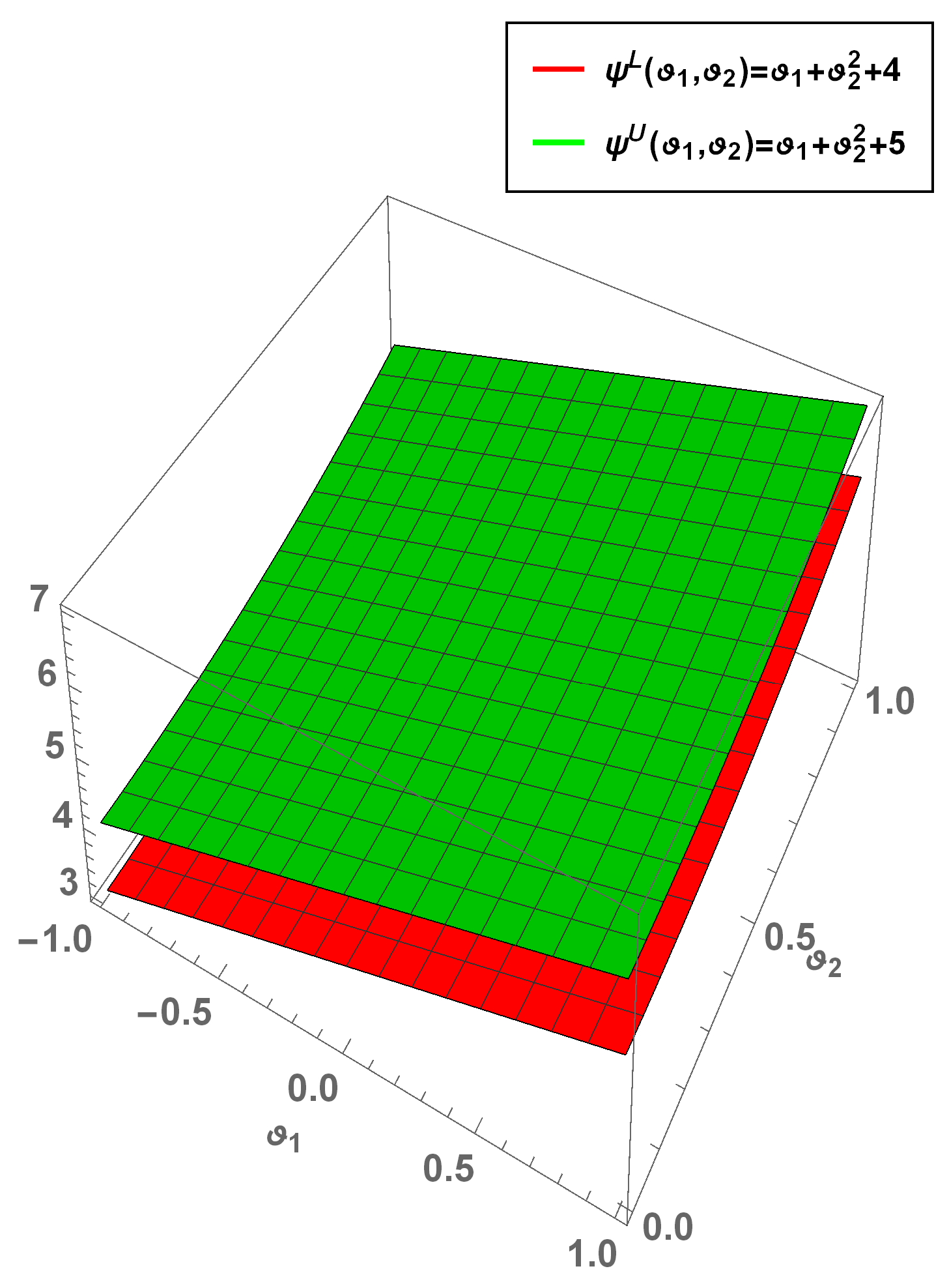
Let ${\Phi }_1=[-0.5,0]$, ${\Phi }_2=[-1,1]$ and $\mathcal{C}={\mathcal{R}}_{+}$. Let ${\Psi }^{\mathcal{L}},{\Psi }^{\mathcal{U}}:{\mathcal{R}}^2\to \mathcal{R}$ and $\phi :{\mathcal{R}}^2\times {\mathcal{R}}^2\to {\mathcal{R}}^2$. One can validate that the robust feasible set is $\mathbb{H}=[-1,1]\times {\mathcal{R}}_{+}$. Then, $\partial {\psi }^{\mathcal{L}}{({\vartheta }_1,{\vartheta }_2)}^T=\left(\begin{array}{c}1\\ \\ 1\end{array}\right)=\partial {\psi }^{\mathcal{U}}{({\vartheta }_1,{\vartheta }_2)}^T$ and ${\partial }_{{\vartheta }_0}\phi \left({\overline{\vartheta }}_1,{\overline{\vartheta }}_2,\overline{\varrho }\right)=\left(\begin{array}{cc}-4& 0\\ 0& -1\end{array}\right).$ One can easily verify that $({\Psi }^{\mathcal{L}},{\Psi }^{\mathcal{U}},\phi )$ is type II $(C,C,R_{+}^{m_0})$-generalized convex at ${\overline{\vartheta }}_0=({\overline{\vartheta }}_1,{\overline{\vartheta }}_2)=(-1,0)$. Moreover, there exists ${\overline{\mu }}^{\mathcal{L}}=1/2={\overline{\mu }}^{\mathcal{U}}$, where ${\overline{\mu }}^{\mathcal{L}},{\overline{\mu }}^{\mathcal{U}}\in C^{*}\backslash \left\{0\right\}$ and $\overline{\gamma }={(1/4,1)}^T\in R_{+}^2$, $\overline{\varrho }=0\in \Phi$. It can be easily verified that

$$0\in \left\{\partial {\Psi }^{\mathcal{L}}{({\overline{\vartheta }}_1,{\overline{\vartheta }}_2)}^T{\overline{\mu }}^{\mathcal{L}}+\partial {\Psi }^{\mathcal{U}}{({\overline{\vartheta }}_1,{\overline{\vartheta }}_2)}^T{\overline{\mu }}^{\mathcal{U}}+{\partial }_{{\vartheta }_0}\phi {\left({\overline{\vartheta }}_1,{\overline{\vartheta }}_2,\overline{\varrho }\right)}^T\overline{\gamma }\right\},$$

$${\overline{\gamma }}^T\phi ({\overline{\vartheta }}_1,{\overline{\vartheta }}_2,\overline{\varrho })=0.$$

Then $\overline{\vartheta }=(-1,0)\in \mathbb{H}$ is a robust $\mathcal{LU}$ -optimal solution of (UCIVOP-1) (See Figure 1).

Theorem 3

(Sufficient $\mathcal{LU}$-optimality conditions). Assume that there exist ${\overline{\mu }}^{\mathcal{L}},{\overline{\mu }}^{\mathcal{U}}\in {\mathcal{C}}^{*}\backslash \left\{0\right\}$, $\overline{\gamma }\in {\mathcal{R}}_{+}^{m_0}$ and $\overline{\varrho }\in \Phi$ such that

$$0\in \left\{\partial {\Psi }^{\mathcal{L}}{\left({\overline{\vartheta }}_0\right)}^T{\overline{\mu }}^{\mathcal{L}}+\partial {\Psi }^{\mathcal{U}}{\left({\overline{\vartheta }}_0\right)}^T{\overline{\mu }}^{\mathcal{U}}+{\partial }_{{\vartheta }_0}\phi ({{\overline{\vartheta }}_0,\overline{\varrho })}^T\overline{\gamma }\right\},$$

(9)

$${\overline{\gamma }}^T\phi ({\overline{\vartheta }}_0,\overline{\varrho })=0.$$

(10)

• (i). If $({\Psi }^{\mathcal{L}},{\Psi }^{\mathcal{U}},\phi )$ is type I $(\mathcal{C},\mathcal{C},{\mathcal{R}}_{+}^{m_0})$-pseudo convex at ${\overline{\vartheta }}_0\in \mathbb{H}$, then ${\overline{\vartheta }}_0$ is a robust $\mathcal{LU}$-optimal solution.
• (ii). If $({\Psi }^{\mathcal{L}},{\Psi }^{\mathcal{U}},\phi )$ is type II $(\mathcal{C},\mathcal{C},{\mathcal{R}}_{+}^{m_0})$-pseudo convex at ${\overline{\vartheta }}_0\in \mathbb{H}$, then ${\overline{\vartheta }}_0$ is a robust $\mathcal{LU}$-optimal solution.

Proof. 

Firstly we validate (i).

Suppose ${\overline{\vartheta }}_0$ is not a robust $\mathcal{LU}$-optimal solution of (UCIVOP), then there exists ${\widehat{\vartheta }}_0\in \mathbb{H}$ such that

$$\Psi \left({\widehat{\vartheta }}_0\right){<}_{\mathcal{LU}}\Psi \left({\overline{\vartheta }}_0\right).$$

That is,

$$\begin{array}{cc}\hfill {\Psi }^{\mathcal{L}}\left({\widehat{\vartheta }}_0\right)& <{\Psi }^{\mathcal{L}}\left({\overline{\vartheta }}_0\right)\hfill \\ \hfill {\Psi }^{\mathcal{U}}\left({\widehat{\vartheta }}_0\right)& <{\Psi }^{\mathcal{U}}\left({\overline{\vartheta }}_0\right),\hfill \end{array}$$

or

$$\begin{array}{cc}\hfill {\Psi }^{\mathcal{L}}\left({\widehat{\vartheta }}_0\right)& \le {\Psi }^{\mathcal{L}}\left({\overline{\vartheta }}_0\right)\hfill \\ \hfill {\Psi }^{\mathcal{U}}\left({\widehat{\vartheta }}_0\right)& <{\Psi }^{\mathcal{U}}\left({\overline{\vartheta }}_0\right),\hfill \end{array}$$

or

$$\begin{array}{cc}\hfill {\Psi }^{\mathcal{L}}\left({\widehat{\vartheta }}_0\right)& <{\Psi }^{\mathcal{L}}\left({\overline{\vartheta }}_0\right)\hfill \\ \hfill {\Psi }^{\mathcal{U}}\left({\widehat{\vartheta }}_0\right)& \le {\Psi }^{\mathcal{U}}\left({\overline{\vartheta }}_0\right).\hfill \end{array}$$

Since ${\overline{\mu }}^{\mathcal{L}}\ge 0$, ${\overline{\mu }}^{\mathcal{U}}\ge 0$, then the preceeding inequalities together yield

$${\overline{\mu }}^{\mathcal{L}}[{\Psi }^{\mathcal{L}}\left({\widehat{\vartheta }}_0\right)-{\Psi }^{\mathcal{L}}\left({\overline{\vartheta }}_0\right)]+{\overline{\mu }}^{\mathcal{U}}[{\Psi }^{\mathcal{U}}\left({\widehat{\vartheta }}_0\right)-{\Psi }^{\mathcal{U}}\left({\overline{\vartheta }}_0\right)]<0.$$

(11)

By virtue of (9), there exist ${\vartheta }_1\in \partial \left({\overline{\mu }}^{\mathcal{L}}{\Psi }^{\mathcal{L}}\right)\left({\overline{\vartheta }}_0\right)$, ${\vartheta }_2\in \partial \left({\overline{\mu }}^{\mathcal{U}}{\Psi }^{\mathcal{U}}\right)\left({\overline{\vartheta }}_0\right)$, ${\varpi }_1\in {\partial }_{{\vartheta }_0}\phi {\left({\overline{\vartheta }}_0,\overline{\varrho }\right)}^T\overline{\gamma }$ such that

$${\vartheta }_1+{\vartheta }_2+{\varpi }_1=0.$$

(12)

Since $({\Psi }^{\mathcal{L}},{\Psi }^{\mathcal{U}},\phi )$ is type I $(\mathcal{C},\mathcal{C},{\mathcal{R}}_{+}^{m_0})$-pseudo convex at ${\overline{\vartheta }}_0$, for any ${\widehat{\vartheta }}_0$ and ${\overline{\mu }}^{\mathcal{L}},{\overline{\mu }}^{\mathcal{U}}\in {\mathcal{C}}^{*}\backslash \left\{0\right\}$ the following hold:

$$\begin{array}{cc}\hfill {\overline{\mu }}^{\mathcal{L}}{\Psi }^L\left({\widehat{\vartheta }}_0\right)& <{\overline{\mu }}^{\mathcal{L}}{\Psi }^{\mathcal{L}}\left({\overline{\vartheta }}_0\right)\Rightarrow A^{\mathcal{L}}({\widehat{\vartheta }}_0-{\overline{\vartheta }}_0)<0,\forall A^L\in \partial \left({\overline{\mu }}^{\mathcal{L}}{\Psi }^{\mathcal{L}}\right)\left({\overline{\vartheta }}_0\right).\hfill \end{array}$$

(13)

$$\begin{array}{cc}\hfill {\overline{\mu }}^{\mathcal{U}}{\Psi }^{\mathcal{U}}\left({\widehat{\vartheta }}_0\right)& <{\overline{\mu }}^{\mathcal{U}}{\Psi }^{\mathcal{U}}\left(\overline{{\vartheta }_0}\right)\Rightarrow A^{\mathcal{U}}({\widehat{\vartheta }}_0-{\overline{\vartheta }}_0)<0,\forall A^{\mathcal{U}}\in \partial \left({\overline{\mu }}^{\mathcal{U}}{\Psi }^{\mathcal{U}}\right)\left({\overline{\vartheta }}_0\right).\hfill \end{array}$$

(14)

$$\begin{array}{c}\hfill \phi ({\widehat{\vartheta }}_0,\overline{\varrho })\le \phi ({\overline{\vartheta }}_0,\overline{\varrho })\Rightarrow B^T({\widehat{\vartheta }}_0-{\overline{\vartheta }}_0)\le 0,\forall B\in {\partial }_{{\vartheta }_0}\phi ({\overline{\vartheta }}_0,\overline{\varrho }).\end{array}$$

(15)

By using the inequalities (11), (13) and (14), we get

$$[A^{\mathcal{L}}+A^{\mathcal{U}}]({\widehat{\vartheta }}_0-{\overline{\vartheta }}_0)<0.$$

(16)

The inequality (16) along with (12) gives

$$-{\varpi }_1({\widehat{\vartheta }}_0-{\overline{\vartheta }}_0)<0.$$

(17)

Since ${\varpi }_1\in {\partial }_{{\vartheta }_0}\phi ({{\overline{\vartheta }}_0,\overline{\varrho })}^T\overline{\gamma }$, we get ${\varpi }_1=B_0^T\overline{\gamma }$, for some $B_0\in {\partial }_{{\vartheta }_0}\phi ({\overline{\vartheta }}_0,\overline{\varrho })$. Thus,

$$-B_0^T\overline{\gamma }({\widehat{\vartheta }}_0-{\overline{\vartheta }}_0)<0,\mathrm{f}\mathrm{o}\mathrm{r} \mathrm{s}\mathrm{o}\mathrm{m}\mathrm{e}{B}_0\in {\partial }_{{\vartheta }_0}\phi ({\overline{\vartheta }}_0,\overline{\varrho }).$$

(18)

Since ${\overline{\vartheta }}_0\in \mathbb{H}$ and using (10) in the inequality (15) with $\overline{\gamma }\in {\mathcal{R}}_{+}^{m_0}$, we obtain

$$B^T\overline{\gamma }({\widehat{\vartheta }}_0-{\overline{\vartheta }}_0)\le 0,\forall B\in {\partial }_{{\vartheta }_0}\phi ({\overline{\vartheta }}_0,\overline{\varrho }).$$

This is a contradiction to (18).

Assertion (ii) is proved similar to part (i) by using the type II pseudo convexity of $({\Psi }^{\mathcal{L}},{\Psi }^{\mathcal{U}},\phi )$ at ${\overline{\vartheta }}_0$. □

4. Wolfe Type Robust Dual Problem

Let us examine the subsequent Wolfe type robust dual problem for (UCIVOP).

$$\begin{array}{cc}\hfill \left(\mathrm{W}\mathrm{I}\mathrm{R}\mathrm{D}\right)& \underset{({\varpi }_0,\varrho ,{\mu }^{\mathcal{L}},{\mu }^{\mathcal{U}},\gamma )}{max}\left(\Psi \left({\varpi }_0\right)+{\gamma }^T\phi ({\varpi }_0,\varrho )\right)=\left\{[{\Psi }^{\mathcal{L}}\left({\varpi }_0\right),{\Psi }^{\mathcal{U}}\left({\varpi }_0\right)]+{\gamma }^T\phi ({\varpi }_0,\varrho )\right\}\hfill \\ \hfill & \mathrm{s}\mathrm{u}\mathrm{b}\mathrm{j}\mathrm{e}\mathrm{c}\mathrm{t}\mathrm{ }\mathrm{t}\mathrm{o}\hfill \\ \hfill & 0\in \left\{\partial {\Psi }^{\mathcal{L}}{\left({\varpi }_0\right)}^T{\mu }^{\mathcal{L}}+\partial {\Psi }^{\mathcal{U}}{\left({\varpi }_0\right)}^T{\mu }^{\mathcal{U}}+{\partial }_{{\vartheta }_0}\phi {({\varpi }_0,\varrho )}^T\gamma \right\},\hfill \\ \hfill & \varrho \in \Phi ,{\mu }^{\mathcal{L}}+{\mu }^{\mathcal{U}}=1,{\mu }^{\mathcal{L}},{\mu }^{\mathcal{U}}\in {\mathcal{C}}^{*}\backslash \left\{0\right\},\gamma \in {\mathcal{R}}_{+}^{m_0}.\hfill \end{array}$$

The robust feasible set of (WIRD) is represented as ${\mathbb{H}}_D^W$, which is the set of all points of the form $({\varpi }_0,\varrho ,{\mu }^{\mathcal{L}},{\mu }^{\mathcal{U}},\gamma )\in {\mathcal{R}}^n\times \Phi \times {\mathcal{C}}^{*}\backslash \left\{0\right\}\times {\mathcal{C}}^{*}\backslash \left\{0\right\}\times {\mathcal{R}}_{+}^{\left(m_0\right)}$ that satisfies the constraints of (WIRD).

Remark 2.

(i). If ${\Psi }^{\mathcal{L}}\left({\varpi }_0\right)={\Psi }^{\mathcal{U}}\left({\varpi }_0\right)$ for all ${\varpi }_0\in {\mathcal{R}}^n$, then (WIRD) model reduces to Wolfe type dual model (WRD) of Chen et al. [42].

(ii). In the absence of uncertain parameter ρ in the constraints, the (WIRD) model reduces to (WD) model of Singh et al. [45].

Definition 9.

The robust feasible point $({\overline{\varpi }}_0,\overline{\varrho },{\overline{\mu }}^{\mathcal{L}},{\overline{\mu }}^{\mathcal{U}},\overline{\gamma })\in {\mathbb{H}}_D^W$ is called a robust $\mathcal{LU}$-optimal solution of (WIRD), if there does not exist a robust feasible solution $({\varpi }_0,\varrho ,{\mu }^{\mathcal{L}},{\mu }^{\mathcal{U}},\gamma )$ of (WIRD) such that $\Psi \left({\overline{\varpi }}_0\right)+{\overline{\gamma }}^T\phi ({\overline{\varpi }}_0,\overline{\varrho }){<}_{\mathcal{LU}}\Psi \left({\varpi }_0\right)+{\gamma }^T\phi ({\varpi }_0,\varrho )$.

The following section describes the duality results between (UCIVOP) and (WIRD).

Theorem 4

(Weak Duality). Let ${\vartheta }_0\in \mathbb{H}$ and $({\varpi }_0,\varrho ,{\mu }^{\mathcal{L}},{\mu }^{\mathcal{U}},\gamma )\in {\mathbb{H}}_D^W.$ If $({\Psi }^{\mathcal{L}},{\Psi }^{\mathcal{U}},\phi )$ is type II $(\mathcal{C},\mathcal{C},{\mathcal{R}}_{+}^{m_0})$-generalized convex at ${\varpi }_0$, then the subsequent inequality cannot hold:

$$\Psi \left({\vartheta }_0\right){<}_{\mathcal{LU}}\Psi \left({\varpi }_0\right)+{\gamma }^T\phi ({\varpi }_0,\varrho ).$$

Proof. 

Suppose, if possible

$$\Psi \left({\vartheta }_0\right){<}_{\mathcal{LU}}\Psi \left({\varpi }_0\right)+{\gamma }^T\phi ({\varpi }_0,\varrho ).$$

(19)

That is,

$$\begin{array}{cc}\hfill {\Psi }^{\mathcal{L}}\left({\vartheta }_0\right)& <{\Psi }^{\mathcal{L}}\left({\varpi }_0\right)+{\gamma }^T\phi ({\varpi }_0,\varrho )\hfill \\ \hfill {\Psi }^{\mathcal{U}}\left({\vartheta }_0\right)& <{\Psi }^{\mathcal{U}}\left({\varpi }_0\right)+{\gamma }^T\phi ({\varpi }_0,\varrho ),\hfill \end{array}$$

or

$$\begin{array}{cc}\hfill {\Psi }^{\mathcal{L}}\left({\vartheta }_0\right)& \le {\Psi }^{\mathcal{L}}\left({\varpi }_0\right)+{\gamma }^T\phi ({\varpi }_0,\varrho )\hfill \\ \hfill {\Psi }^{\mathcal{U}}\left({\vartheta }_0\right)& <{\Psi }^{\mathcal{U}}\left({\varpi }_0\right)+{\gamma }^T\phi ({\varpi }_0,\varrho ),\hfill \end{array}$$

or

$$\begin{array}{cc}\hfill {\Psi }^{\mathcal{L}}\left({\vartheta }_0\right)& <{\Psi }^{\mathcal{L}}\left({\varpi }_0\right)+{\gamma }^T\phi ({\varpi }_0,\varrho )\hfill \\ \hfill {\Psi }^{\mathcal{U}}\left({\vartheta }_0\right)& \le {\Psi }^{\mathcal{U}}\left({\varpi }_0\right)+{\gamma }^T\phi ({\varpi }_0,\varrho ).\hfill \end{array}$$

Since ${\mu }^{\mathcal{L}}\ge 0$, ${\mu }^{\mathcal{U}}\ge 0$, then the preceeding inequalities together yield

$${\mu }^{\mathcal{L}}[{\Psi }^{\mathcal{L}}\left({\vartheta }_0\right)-{\Psi }^{\mathcal{L}}\left({\varpi }_0\right)]+{\mu }^{\mathcal{U}}[{\Psi }^{\mathcal{U}}\left({\vartheta }_0\right)-{\Psi }^{\mathcal{U}}\left({\varpi }_0\right)]-{\gamma }^T\phi ({\varpi }_0,\varrho )[{\mu }^{\mathcal{L}}+{\mu }^{\mathcal{U}}]<0.$$

(20)

Since $({\varpi }_0,\varrho ,{\mu }^{\mathcal{L}},{\mu }^{\mathcal{U}},\gamma )\in {\mathbb{H}}_D^W$, we obtain ${\mu }^{\mathcal{L}},{\mu }^{\mathcal{U}}\in {\mathcal{C}}^{*}\backslash \left\{0\right\}$, $\gamma \in {\mathcal{R}}_{+}^{m_0}$, $\varrho \in \Phi$,

$$\begin{array}{c}\hfill {\mu }^{\mathcal{L}}+{\mu }^{\mathcal{U}}=1,\end{array}$$

(21)

$$\begin{array}{c}\hfill 0\in \left\{\partial {\Psi }^{\mathcal{L}}{\left({\varpi }_0\right)}^T{\mu }^{\mathcal{L}}+\partial {\Psi }^{\mathcal{U}}{\left({\varpi }_0\right)}^T{\mu }^{\mathcal{U}}+{\partial }_{{\vartheta }_0}\phi {({\varpi }_0,\varrho )}^T\gamma \right\}.\end{array}$$

(22)

By using (21), the inequality (20) gives

$$\begin{array}{c}\hfill {\mu }^{\mathcal{L}}[{\Psi }^{\mathcal{L}}\left({\vartheta }_0\right)-{\Psi }^{\mathcal{L}}\left({\varpi }_0\right)]+{\mu }^{\mathcal{U}}[{\Psi }^U\left({\vartheta }_0\right)-{\Psi }^{\mathcal{U}}\left({\varpi }_0\right)]-{\gamma }^T\phi ({\varpi }_0,\varrho )<0.\end{array}$$

(23)

Since $({\Psi }^{\mathcal{L}},{\Psi }^{\mathcal{U}},\phi )$ is type II $(\mathcal{C},\mathcal{C},{\mathcal{R}}_{+}^{m_0})$-generalized convex at ${\varpi }_0$, then there exists $\xi \in \mathcal{R}$ such that

$$\begin{array}{c}\hfill {\Psi }^{\mathcal{L}}\left({\vartheta }_0\right)-{\Psi }^{\mathcal{L}}\left({\varpi }_0\right)-A^{\mathcal{L}}\xi \in \mathcal{C},\forall A^L\in \partial {\Psi }^{\mathcal{L}}({\varpi }_0),\\ \hfill {\Psi }^{\mathcal{U}}\left({\vartheta }_0\right)-{\Psi }^{\mathcal{U}}\left({\varpi }_0\right)-A^{\mathcal{U}}\xi \in \mathcal{C},\forall A^{\mathcal{U}}\in \partial {\Psi }^{\mathcal{U}}({\varpi }_0),\\ \hfill -\phi ({\varpi }_0,\varrho )-B\xi \in {\mathcal{R}}_{+}^{m_0},\forall B\in {\partial }_{{\vartheta }_0}\phi ({\varpi }_0,\varrho ).\end{array}$$

From the above inequalities, one has

$$\begin{array}{c}\hfill {\mu }^{\mathcal{L}}[{\Psi }^{\mathcal{L}}\left({\vartheta }_0\right)-{\Psi }^{\mathcal{L}}\left({\varpi }_0\right)-A^{\mathcal{L}}\xi ]\ge 0,\forall A^{\mathcal{L}}\in \partial {\Psi }^{\mathcal{L}}({\varpi }_0),\\ \hfill {\mu }^{\mathcal{U}}[{\Psi }^{\mathcal{U}}\left({\vartheta }_0\right)-{\Psi }^{\mathcal{U}}\left({\varpi }_0\right)-A^{\mathcal{U}}\xi ]\ge 0,\forall A^{\mathcal{U}}\in \partial {\Psi }^{\mathcal{U}}({\varpi }_0),\\ \hfill {\gamma }^T[-\phi ({\varpi }_0,\varrho )-B\xi ]\ge 0,\forall B\in {\partial }_{{\vartheta }_0}\phi \left({\varpi }_0,\varrho \right).\end{array}$$

Combining the above inequalities, we get

$$[{\mu }^{\mathcal{L}}{A}^{\mathcal{L}}+{\mu }^{\mathcal{U}}{A}^{\mathcal{U}}+{\gamma }^{T}B]\xi$$

$$\le {\mu }^{\mathcal{L}}[{\Psi }^{\mathcal{L}}\left({\vartheta }_0\right)-{\Psi }^{\mathcal{L}}\left({\varpi }_0\right)]+{\mu }^{\mathcal{U}}[{\Psi }^{\mathcal{U}}\left({\vartheta }_0\right)-{\Psi }^{\mathcal{U}}\left({\varpi }_0\right)]-{\gamma }^T\phi ({\varpi }_0,\varrho ).$$

(24)

By using (23), the inequality(24) implies

$$[{\mu }^L{A}^{\mathcal{L}}+{\mu }^{\mathcal{U}}{A}^{\mathcal{U}}+{\gamma }^{T}B]\xi <0,\forall A^{\mathcal{L}}\in \partial {\Psi }^{\mathcal{L}}({\varpi }_0),\forall A^{\mathcal{U}}\in \partial {\Psi }^{\mathcal{U}}({\varpi }_0),\forall B\in {\partial }_{{\vartheta }_0}\phi \left({\varpi }_0,\varrho \right),$$

which contradicts (22) and hence the theorem. □

We now re-explore Example 1 to demonstrate Theorem 4.

Example 2.

Let us examine the uncertain constrained interval-valued optimization problem.

$$\begin{array}{cc}\hfill (\mathrm{U}\mathrm{C}\mathrm{I}\mathrm{V}\mathrm{O}\mathrm{P}-1)& \underset{{\vartheta }_1,{\vartheta }_2\in \mathcal{R}}{\mathrm{m}\mathrm{i}\mathrm{n}}\Psi \left({\vartheta }_1,{\vartheta }_2\right)=[{\Psi }^{\mathcal{L}}\left({\vartheta }_1,{\vartheta }_2\right),{\Psi }^{\mathcal{U}}\left({\vartheta }_1,{\vartheta }_2\right)]\hfill \\ \hfill & \mathrm{s}\mathrm{u}\mathrm{b}\mathrm{j}\mathrm{e}\mathrm{c}\mathrm{t} \mathrm{t}\mathrm{o}\hfill \\ \hfill & -\phi ({\vartheta }_1,{\vartheta }_2,\varrho )\in {\mathcal{R}}_{+}^2,\mathrm{where}\varrho \in \Phi .\hfill \end{array}$$

Let ${\mathcal{R}}^n,\mathcal{R},{\mathcal{R}}^{m_0},{\mathcal{R}}^p,\mathcal{C},{\Phi }_1,{\Phi }_2,{\Psi }^{\mathcal{L}},{\Psi }^{\mathcal{U}}$ and φ be same as Example 1. The robust counterpart of (UCIVOP-1) is defined as follows:

$$\begin{array}{cc}\hfill (\mathrm{R}\mathrm{I}\mathrm{V}\mathrm{O}\mathrm{P}-1)& \underset{{\vartheta }_1,{\vartheta }_2\in \mathcal{R}}{\mathrm{m}\mathrm{i}\mathrm{n}}\Psi \left({\vartheta }_1,{\vartheta }_2\right)=\left([1,1]{\vartheta }_1+[1,1]{\vartheta }_2^2+[4,5]\right)\hfill \\ \hfill & \mathrm{s}\mathrm{u}\mathrm{b}\mathrm{j}\mathrm{e}\mathrm{c}\mathrm{t} \mathrm{t}\mathrm{o}\hfill \\ \hfill & {\left\{-{{\vartheta }_1}^2+2{\vartheta }_1+3-ln(1+{\varrho }_1),{\vartheta }_2+\left|{\varrho }_2\right|\right\}}^T\in {\mathcal{R}}_{+}^2,\forall \varrho \in \Phi ,\hfill \end{array}$$

where $\varrho =({\varrho }_1,{\varrho }_2)\in \Phi ={\Phi }_1\times {\Phi }_2$. Recall that the robust feasible set of (RIVOP-1) is $\mathbb{H}=[-1,1]\times {\mathcal{R}}_{+}$.

We consider a Wolfe type robust dual problem (WIRD-1) for (RIVOP-1) as follows:

$$\begin{array}{cc}\hfill (\mathrm{W}\mathrm{I}\mathrm{R}\mathrm{D}-1)\underset{({\varpi }_1,{\varpi }_2,\varrho ,{\mu }^{\mathcal{L}},{\mu }^{\mathcal{U}},\gamma )}{max}& \left(\right([1,1]{\varpi }_1+[1,1]{\varpi }_2^2+[4,5])\hfill \\ \hfill & +{\gamma }^T{\left\{{\varpi }_1^2-2{\varpi }_1-3+ln(1+{\varrho }_1),-{\varpi }_2-\left|{\varrho }_2\right|\right\}}^T)\hfill \\ \hfill & \mathrm{s}\mathrm{u}\mathrm{b}\mathrm{j}\mathrm{e}\mathrm{c}\mathrm{t} \mathrm{t}\mathrm{o}\hfill \\ \hfill & 0\in \left\{\partial {\Psi }^{\mathcal{L}}{({\overline{\varpi }}_1,{\overline{\varpi }}_2)}^T{\mu }^{\mathcal{L}}+\partial {\Psi }^{\mathcal{U}}{({\overline{\varpi }}_1,{\overline{\varpi }}_2)}^T{\mu }^{\mathcal{U}}+{\partial }_{{\vartheta }_0}\phi {\left({\overline{\varpi }}_1,{\overline{\varpi }}_2,\overline{\varrho }\right)}^T\gamma \right\},\hfill \end{array}$$

where ${\mu }^{\mathcal{L}}+{\mu }^{\mathcal{U}}=1$, ${\mu }^{\mathcal{L}},{\mu }^{\mathcal{U}}\in {\mathcal{C}}^{*}\backslash \left\{0\right\}$ and $\gamma \in {\mathcal{R}}_{+}^{m_0}$. Again from Example 1, we have $({\vartheta }_1,{\vartheta }_2,\varrho ,{\mu }^{\mathcal{L}},{\mu }^{\mathcal{U}},\gamma )\in {\mathbb{H}}_D^W$ where ${\mu }^{\mathcal{L}}=1/2={\mu }^{\mathcal{U}}$, $\gamma ={(1/4,1)}^T\in {\mathcal{R}}_{+}^2$, $\varrho =0\in \Phi$. For any $({\varpi }_1,{\varpi }_2,\varrho ,{\mu }^{\mathcal{L}},{\mu }^{\mathcal{U}},\gamma )\in {\mathbb{H}}_D^W$, we conclude that ${\mu }^{\mathcal{L}},{\mu }^{\mathcal{U}}\in {\mathcal{C}}^{*}\backslash \left\{0\right\}$, $\gamma =({\gamma }_1$, ${\gamma }_2{)}^T\in {\mathcal{R}}_{+}^2$. Hence, it follows

$$\left(\begin{array}{c}0\\ \\ 0\end{array}\right)=\left(\begin{array}{c}1\\ \\ 2{\varpi }_2\end{array}\right){\mu }^{\mathcal{L}}+\left(\begin{array}{c}1\\ \\ 2{\varpi }_2\end{array}\right){\mu }^{\mathcal{U}}+\left(\begin{array}{cc}2{\varpi }_1-2& 0\\ 0& -1\end{array}\right)\left(\begin{array}{c}{\gamma }_1\\ \\ {\gamma }_2\end{array}\right)$$

From the above equation, we get ${\mu }^{\mathcal{L}}+{\mu }^{\mathcal{U}}+2({\varpi }_1-1){\gamma }_1=0$ and $2{\varpi }_2({\mu }^{\mathcal{L}}+{\mu }^{\mathcal{U}})-{\gamma }_2=0$. Combining these equations along with ${\mu }^{\mathcal{L}},{\mu }^{\mathcal{U}},{\gamma }_1,{\gamma }_2\ge 0$ and ${\mu }^{\mathcal{L}}+{\mu }^{\mathcal{U}}=1$, we obtain ${\varpi }_2\ge 0$, ${\varpi }_1\le 1$. Taking into account ${\varpi }_2\ge 0$, ${\varpi }_1\le 1$ and $\forall ({\varpi }_1,{\varpi }_2,\varrho ,{\mu }^{\mathcal{L}},{\mu }^{\mathcal{U}},\gamma )\in {\mathbb{H}}_D^W$, we have,

$$\begin{array}{c}\hfill {\mu }^{\mathcal{L}}[{\Psi }^{\mathcal{L}}({\vartheta }_1,{\vartheta }_2)-{\Psi }^{\mathcal{L}}({\varpi }_1,{\varpi }_2)]+{\mu }^{\mathcal{U}}[{\Psi }^{\mathcal{U}}({\vartheta }_1,{\vartheta }_2)-{\Psi }^{\mathcal{U}}({\varpi }_1,{\varpi }_2)]\\ \hfill -({\mu }^{\mathcal{L}}+{\mu }^{\mathcal{U}}){\gamma }^T\phi ({\varpi }_1,{\varpi }_2,\varrho )\\ \hfill =-1/4-3{\varpi }_1/2-{\varpi }_1^2/4-{\varpi }_2^2+{\varpi }_2-ln(1+{\varrho }_1)/4+\left|w_2\right|\nless 0.\end{array}$$

Therefore, weak duality theorem of (WIRD-1) holds.

Theorem 5

(Strong Duality). Let ${\overline{\vartheta }}_0$ be a robust $\mathcal{LU}$-optimal solution of (UCIVOP) and (GRSCQ) hold. Assume that φ satisfy the Assumption $\mathbb{D}$, ϕ is ${\mathcal{R}}_{+}$-convexlike and ${\Psi }^{\mathcal{L}}$, ${\Psi }^{\mathcal{U}}$ be $\mathcal{C}$-convexlike. Then, there exist $\overline{\varrho }\in \Phi$, ${\overline{\mu }}^{\mathcal{L}},{\overline{\mu }}^{\mathcal{U}}\in {\mathcal{C}}^{*}\backslash \left\{0\right\}$, $\overline{\gamma }\in R_{+}^{m_0}$ such that $({\overline{\vartheta }}_0,\overline{\varrho },{\overline{\mu }}^{\mathcal{L}},{\overline{\mu }}^{\mathcal{U}},\overline{\gamma })\in {\mathbb{H}}_D^W$. Furthermore, if $({\Psi }^{\mathcal{L}},{\Psi }^{\mathcal{U}},\phi )$ is type II $(\mathcal{C},\mathcal{C},{\mathcal{R}}_{+}^{m_0})$-generalized convex at ${\varpi }_0$, where $({\varpi }_0,\varrho ,{\mu }^{\mathcal{L}},{\mu }^{\mathcal{U}},\gamma )\in {\mathbb{H}}_D^W$ then $({\overline{\vartheta }}_0,\overline{\varrho },{\overline{\mu }}^{\mathcal{L}},{\overline{\mu }}^{\mathcal{U}},\overline{\gamma })$ is a robust $\mathcal{LU}$-optimal solution of (WIRD).

Proof. 

As a result of Theorem 1, there exist $\overline{\varrho }\in \Phi$, ${\overline{\mu }}^{\mathcal{L}},{\overline{\mu }}^{\mathcal{U}}\in {\mathcal{C}}^{*}\backslash \left\{0\right\}$, $\overline{\gamma }\in {\mathcal{R}}_{+}^{m_0}$ such that $({\overline{\vartheta }}_0,\overline{\varrho },{\overline{\mu }}^{\mathcal{L}},{\overline{\mu }}^{\mathcal{U}},\overline{\gamma })\in {\mathbb{H}}_D^W$ and

$${\overline{\gamma }}^T\phi ({\overline{\vartheta }}_0,\overline{\varrho })=0.$$

(25)

By Theorem 4, the subsequent inequality does not hold:

$$\Psi \left({\overline{\vartheta }}_0\right){<}_{\mathcal{LU}}\Psi \left({\varpi }_0\right)+{\gamma }^T\phi ({\varpi }_0,\varrho ),\forall ({\varpi }_0,\varrho ,{\mu }^{\mathcal{L}},{\mu }^{\mathcal{U}},\gamma )\in {\mathbb{H}}_D^W.$$

This implies $({\overline{\vartheta }}_0,\overline{\varrho },{\overline{\mu }}^{\mathcal{L}},{\overline{\mu }}^{\mathcal{U}},\overline{\gamma })$ is a robust $\mathcal{LU}$-optimal solution of (WIRD). □

Theorem 6

(Converse Duality). Let $({\varpi }_0,\varrho ,{\mu }^{\mathcal{L}},{\overline{\mu }}^L,{\overline{\mu }}^{\mathcal{U}},\overline{\gamma })$ be a robust $\mathcal{LU}$-optimal solution of (WIRD) with ${\overline{\varpi }}_0\in \mathbb{H}$. If $({\Psi }^L,{\Psi }^U,\phi )$ is type II $(\mathcal{C},\mathcal{C},{\mathcal{R}}_{+}^{m_0})$-generalized convex at ${\overline{\varpi }}_0$, then ${\overline{\varpi }}_0$ is a robust $\mathcal{LU}$-optimal solution of (UCIVOP).

Proof. 

Since $({\overline{\varpi }}_0,\overline{\varrho },{\overline{\mu }}^{\mathcal{L}},{\overline{\mu }}^{\mathcal{U}},\overline{\gamma })$ is a robust $\mathcal{LU}$-optimal solution of (WIRD) and ${\overline{\varpi }}_0\in \mathbb{H}$. Then, it follows from Theorem 4, the subsequent inequality does not hold:

$$\Psi \left({\vartheta }_0\right){<}_{\mathcal{LU}}\Psi \left({\overline{\varpi }}_0\right)+{\overline{\gamma }}^T\phi ({\overline{\varpi }}_0,\overline{\varrho }),\forall {\vartheta }_0\in \mathbb{H}.$$

This implies, the subsequent inequality does not hold: $\Psi \left({\vartheta }_0\right){<}_{\mathcal{LU}}\Psi \left({\overline{\varpi }}_0\right)$.

Hence, ${\overline{\varpi }}_0$ is a robust $\mathcal{LU}$-optimal solution of (UCIVOP). □

5. Mond-Weir Type Robust Dual Problem

Let us examine the subsequent Mond-Weir type robust dual problem for (UCIVOP).

$$\begin{array}{cc}\hfill \left(\mathrm{M}\mathrm{W}\mathrm{I}\mathrm{V}\mathrm{R}\mathrm{D}\right)& \underset{({\varpi }_0,\varrho ,{\mu }^{\mathcal{L}},{\mu }^{\mathcal{U}},\gamma )}{max}\Psi \left({\varpi }_0\right)=[{\Psi }^{\mathcal{L}}\left({\varpi }_0\right),{\Psi }^{\mathcal{U}}\left({\varpi }_0\right)]\hfill \\ \hfill & \mathrm{s}\mathrm{u}\mathrm{b}\mathrm{j}\mathrm{e}\mathrm{c}\mathrm{t} \mathrm{t}\mathrm{o}\hfill \\ \hfill & 0\in \left\{\partial {\Psi }^{\mathcal{L}}{\left({\varpi }_0\right)}^T{\mu }^{\mathcal{L}}+\partial {\Psi }^{\mathcal{U}}{\left({\varpi }_0\right)}^T{\mu }^{\mathcal{U}}+{\partial }_{{\vartheta }_0}\phi {({\varpi }_0,\varrho )}^T\gamma \right\},\hfill \\ \hfill & {\gamma }^T\phi ({\varpi }_0,\varrho )\ge 0,\varrho \in \Phi ,\hfill \\ \hfill & {\mu }^{\mathcal{L}},{\mu }^{\mathcal{U}}\in {\mathcal{C}}^{*}\backslash \left\{0\right\},\gamma \in {\mathcal{R}}_{+}^{m_0}.\hfill \end{array}$$

It is worth mentioning that (MWIVRD) is viewed as a likely version to the Mond-Weir type robust dual problem of (UCIVOP).

$$\begin{array}{cc}\hfill \left(\mathrm{M}\mathrm{W}\mathrm{I}\mathrm{V}\mathrm{R}\mathrm{D}\right)& \underset{({\varpi }_0,\varrho ,{\mu }^{\mathcal{L}},{\mu }^{\mathcal{U}},\gamma )}{max}\Psi \left({\varpi }_0\right)=[{\Psi }^{\mathcal{L}}\left({\varpi }_0\right),{\Psi }^{\mathcal{U}}\left({\varpi }_0\right)]\hfill \\ \hfill & \mathrm{s}\mathrm{u}\mathrm{b}\mathrm{j}\mathrm{e}\mathrm{c}\mathrm{t} \mathrm{t}\mathrm{o}\hfill \\ \hfill & 0\in \left\{\partial {\Psi }^{\mathcal{L}}{\left({\varpi }_0\right)}^T{\mu }^{\mathcal{L}}+\partial {\Psi }^{\mathcal{U}}{\left({\varpi }_0\right)}^T{\mu }^{\mathcal{U}}+{\partial }_{{\vartheta }_0}\phi {({\varpi }_0,\varrho )}^T\gamma \right\},\hfill \\ \hfill & {\gamma }^T\phi ({\varpi }_0,\varrho )\ge 0,\hfill \\ \hfill & {\mu }^{\mathcal{L}},{\mu }^{\mathcal{U}}\in {\mathcal{C}}^{*}\backslash \left\{0\right\},\gamma \in {\mathcal{R}}_{+}^{m_0},\hfill \end{array}$$

where $\varrho \in \Phi$ is an uncertain parameter.

The robust feasible set of (MWIVRD) is denoted by ${\mathbb{H}}_D^{MW}$, which is the set of all points of the form $({\varpi }_0,\varrho ,{\mu }^{\mathcal{L}},{\mu }^{\mathcal{U}},\gamma )\in {\mathcal{R}}^n\times \Phi \times {\mathcal{C}}^{*}\backslash \left\{0\right\}\times {\mathcal{C}}^{*}\backslash \left\{0\right\}\times {\mathcal{R}}_{+}^{\left(m_0\right)}$ that satisfies the constraints of (MWIVRD).

Remark 3.

(i). If ${\Psi }^{\mathcal{L}}\left({\varpi }_0\right)={\Psi }^{\mathcal{U}}\left({\varpi }_0\right)$ for all ${\varpi }_0\in {\mathcal{R}}^n$, then (MWIVRD) reduces to Mond-Wier type dual model (MWRD) of Chen et al. [42].

(ii). In the absence of uncertain parameter ρ in the constraints, the (MWIVRD) reduces to (MWD) model of Singh et al. [45].

Definition 10.

The robust feasible point $({\overline{\varpi }}_0,\overline{\varrho },{\overline{\mu }}^{\mathcal{L}},{\overline{\mu }}^{\mathcal{U}},\overline{\gamma })\in {\mathbb{H}}_D^{MW}$ is called a robust $\mathcal{LU}$-optimal solution of (MWIVRD), if there does not exist a robust feasible solution $({\varpi }_0,\varrho ,{\mu }^{\mathcal{L}},{\mu }^{\mathcal{U}},\gamma )$ of (MWIVRD) such that $\Psi \left({\overline{\varpi }}_0\right){<}_{\mathcal{LU}}\Psi \left({\varpi }_0\right).$

The following section describes the duality results between (UCIVOP) and (MWIVRD).

Theorem 7

(Weak Duality). Let ${\vartheta }_0\in \mathbb{H}$ and $({\varpi }_0,\varrho ,{\mu }^{\mathcal{L}},{\mu }^{\mathcal{U}},\gamma )\in {\mathbb{H}}_D^{MW}$.

• (i). If $({\Psi }^{\mathcal{L}},{\Psi }^{\mathcal{U}},\phi )$ is type I $(\mathcal{C},\mathcal{C},{\mathcal{R}}_{+}^{m_0})$-pseudo convex at ${\varpi }_0$, then the subsequent inequality cannot hold:

  $$\Psi \left({\vartheta }_0\right){<}_{\mathcal{LU}}\Psi \left({\varpi }_0\right).$$
• (ii). If $({\Psi }^{\mathcal{L}},{\Psi }^{\mathcal{U}},\phi )$ is type II $(\mathcal{C},\mathcal{C},{\mathcal{R}}_{+}^{m_0})$-pseudo convex at ${\varpi }_0$, then the subsequent inequality cannot hold:

  $$\Psi \left({\vartheta }_0\right){<}_{\mathcal{LU}}\Psi \left({\varpi }_0\right).$$

Proof. 

Firstly we validate (i).

Suppose, if possible

$$\Psi \left({\vartheta }_0\right){<}_{\mathcal{LU}}\Psi \left({\varpi }_0\right).$$

That is,

$$\begin{array}{cc}\hfill {\Psi }^{\mathcal{L}}\left({\vartheta }_0\right)& <{\Psi }^{\mathcal{L}}\left({\varpi }_0\right)\hfill \\ \hfill {\Psi }^{\mathcal{U}}\left({\vartheta }_0\right)& <{\Psi }^{\mathcal{U}}\left({\varpi }_0\right),\hfill \end{array}$$

or

$$\begin{array}{cc}\hfill {\Psi }^{\mathcal{L}}\left({\vartheta }_0\right)& \le {\Psi }^{\mathcal{L}}\left({\varpi }_0\right)\hfill \\ \hfill {\Psi }^{\mathcal{U}}\left({\vartheta }_0\right)& <{\Psi }^{\mathcal{U}}\left({\varpi }_0\right),\hfill \end{array}$$

or

$$\begin{array}{cc}\hfill {\Psi }^{\mathcal{L}}\left({\vartheta }_0\right)& <{\Psi }^{\mathcal{L}}\left({\varpi }_0\right)\hfill \\ \hfill {\Psi }^{\mathcal{U}}\left({\vartheta }_0\right)& \le {\Psi }^{\mathcal{U}}\left({\varpi }_0\right).\hfill \end{array}$$

Since ${\mu }^{\mathcal{L}}\ge 0$, ${\mu }^{\mathcal{U}}\ge 0$, then the preceeding inequalities together yield

$${\mu }^L[{\Psi }^{\mathcal{L}}\left({\vartheta }_0\right)-{\Psi }^{\mathcal{L}}\left({\varpi }_0\right)]+{\mu }^{\mathcal{U}}[{\Psi }^{\mathcal{U}}\left({\vartheta }_0\right)-{\Psi }^{\mathcal{U}}\left({\varpi }_0\right)]<0.$$

(26)

Since $({\varpi }_0,\varrho ,{\mu }^{\mathcal{L}},{\mu }^{\mathcal{U}},\gamma )\in {\mathbb{H}}_D^{MW}$, there exist ${\mu }^{\mathcal{L}},{\mu }^{\mathcal{U}}\in {\mathcal{C}}^{*}\backslash \left\{0\right\}$, $\gamma \in {\mathcal{R}}_{+}^{m_0}$, $\varrho \in \Phi$ such that

$$\begin{array}{c}\hfill {\gamma }^T\phi ({\varpi }_0,\varrho )\ge 0,\end{array}$$

(27)

$$\begin{array}{c}\hfill 0\in \left\{\partial {\Psi }^{\mathcal{L}}{\left({\varpi }_0\right)}^T{\mu }^{\mathcal{L}}+\partial {\Psi }^{\mathcal{U}}{\left({\varpi }_0\right)}^T{\mu }^{\mathcal{U}}+{\partial }_{{\vartheta }_0}\phi {({\varpi }_0,\varrho )}^T\gamma \right\}.\end{array}$$

(28)

By virtue of (28), there exist ${\vartheta }_1\in \partial \left({\mu }^{\mathcal{L}}{\Psi }^{\mathcal{L}}\right)\left({\varpi }_0\right)$, ${\vartheta }_2\in \partial \left({\mu }^{\mathcal{U}}{\Psi }^{\mathcal{U}}\right)\left({\varpi }_0\right)$, ${\varpi }_1\in {\partial }_{{\vartheta }_0}\phi {\left({\varpi }_0,\varrho \right)}^T\gamma$ such that

$${\vartheta }_1+{\vartheta }_2+{\varpi }_1=0.$$

(29)

Since $({\Psi }^{\mathcal{L}},{\Psi }^{\mathcal{U}},\phi )$ is type I $(\mathcal{C},\mathcal{C},{\mathcal{R}}_{+}^{m_0})$-pseudo convex at ${\varpi }_0$, for any ${\vartheta }_0$ and ${\mu }^{\mathcal{L}},{\mu }^{\mathcal{U}}\in {\mathcal{C}}^{*}\backslash \left\{0\right\}$ the following hold:

$$\begin{array}{cc}\hfill {\mu }^{\mathcal{L}}{\Psi }^{\mathcal{L}}\left({\vartheta }_0\right)& <{\mu }^{\mathcal{L}}{\Psi }^{\mathcal{L}}\left({\varpi }_0\right)\Rightarrow A^{\mathcal{L}}({\vartheta }_0-{\varpi }_0)<0,\forall A^{\mathcal{L}}\in \partial \left({\mu }^{\mathcal{L}}{\Psi }^{\mathcal{L}}\right)\left({\varpi }_0\right).\hfill \end{array}$$

(30)

$$\begin{array}{cc}\hfill {\mu }^{\mathcal{U}}{\Psi }^{\mathcal{U}}\left({\vartheta }_0\right)& <{\mu }^{\mathcal{U}}{\Psi }^{\mathcal{U}}\left({\varpi }_0\right)\Rightarrow A^{\mathcal{U}}({\vartheta }_0-{\varpi }_0)<0,\forall A^{\mathcal{U}}\in \partial \left({\mu }^{\mathcal{U}}{\Psi }^{\mathcal{U}}\right)\left({\varpi }_0\right).\hfill \end{array}$$

(31)

$$\begin{array}{c}\hfill \phi ({\vartheta }_0,\varrho )\le \phi ({\varpi }_0,\varrho )\Rightarrow B^T({\vartheta }_0-{\varpi }_0)\le 0,\forall B\in {\partial }_{{\vartheta }_0}\phi ({\varpi }_0,\varrho ).\end{array}$$

(32)

By using the inequalities (26), (30) and (31), we obtain

$$[A^{\mathcal{L}}+A^{\mathcal{U}}]({\vartheta }_0-{\varpi }_0)<0.$$

(33)

The inequality (33) along with (29) gives

$$-{\varpi }_1({\vartheta }_0-{\varpi }_0)<0.$$

(34)

Since ${\varpi }_1\in {\partial }_{{\vartheta }_0}\phi ({{\varpi }_0,\varrho )}^T\gamma$, we get ${\varpi }_1=B_0^T\gamma$, for some $B_0\in {\partial }_{{\vartheta }_0}\phi ({\varpi }_0,\varrho )$.

Thus,

$$-B_0^T\gamma ({\vartheta }_0-{\varpi }_0)<0,\mathrm{f}\mathrm{o}\mathrm{r}\mathrm{s}\mathrm{o}\mathrm{m}\mathrm{e}{B}_0\in {\partial }_{{\vartheta }_0}\phi ({\varpi }_0,\varrho ).$$

(35)

Since ${\vartheta }_0\in \mathbb{H}$ and using (27) in the inequality (32) with $\gamma \in {\mathcal{R}}_{+}^{m_0}$, we have

$$B^T\gamma ({\vartheta }_0-{\varpi }_0)\le 0,\forall B\in {\partial }_{{\vartheta }_0}\phi ({\varpi }_0,\varrho ).$$

This is a contradiction to (35).

Assertion (ii) is proved similar to part (i) by using the type II pseudo convexity of $({\Psi }^{\mathcal{L}},{\Psi }^{\mathcal{U}},\phi )$ at ${\varpi }_0$. □

We demonstrate weak duality theorem by the subsequent illustration.

Example 3.

Consider the subsequent uncertain constrained interval-valued optimization problem.

$$\begin{array}{cc}\hfill (\mathrm{U}\mathrm{C}\mathrm{I}\mathrm{V}\mathrm{O}\mathrm{P}-2)& \underset{{\vartheta }_1,{\vartheta }_2\in \mathcal{R}}{\mathrm{m}\mathrm{i}\mathrm{n}}\Psi \left({\vartheta }_1,{\vartheta }_2\right)=[{\Psi }^{\mathcal{L}}\left({\vartheta }_1,{\vartheta }_2\right),{\Psi }^{\mathcal{U}}\left({\vartheta }_1,{\vartheta }_2\right)]\hfill \\ \hfill & \mathrm{s}\mathrm{u}\mathrm{b}\mathrm{j}\mathrm{e}\mathrm{c}\mathrm{t} \mathrm{t}\mathrm{o}\hfill \\ \hfill & -\phi ({\vartheta }_1,{\vartheta }_2,\varrho )\in {\mathcal{R}}_{+}^2,\mathrm{w}\mathrm{h}\mathrm{e}\mathrm{r}\mathrm{e}\varrho \in \Phi .\hfill \end{array}$$

The robust counterpart of (UCIVOP-2) is defined as follows:

$$\begin{array}{cc}\hfill (\mathrm{R}\mathrm{I}\mathrm{V}\mathrm{O}\mathrm{P}-2)& \underset{{\vartheta }_1,{\vartheta }_2\in \mathcal{R}}{\mathrm{m}\mathrm{i}\mathrm{n}}\Psi \left({\vartheta }_1,{\vartheta }_2\right)=\left([1,1]{\vartheta }_1+[1,1]{\vartheta }_2^3+[4,5]\right)\hfill \\ \hfill & \mathrm{s}\mathrm{u}\mathrm{b}\mathrm{j}\mathrm{e}\mathrm{c}\mathrm{t} \mathrm{t}\mathrm{o}\hfill \\ \hfill & {\left\{-{{\vartheta }_1}^2+2{\vartheta }_1+3-ln(1+{\varrho }_1),{\vartheta }_2+\left|{\varrho }_2\right|\right\}}^T\in {\mathcal{R}}_{+}^2,\forall \varrho \in \Phi ,\hfill \end{array}$$

where $\varrho =({\varrho }_1,{\varrho }_2)\in \Phi ={\Phi }_1\times {\Phi }_2$. Clearly, the robust feasible set of (RIVOP-2) is $\mathbb{H}=[-1,1]\times {\mathcal{R}}_{+}$.

We consider a Mond-Weir type robust dual problem (MWIVRD-2) for (RIVOP-2) as follows:

$$\begin{array}{cc}\hfill (\mathrm{M}\mathrm{W}\mathrm{I}\mathrm{V}\mathrm{R}\mathrm{D}-2)\underset{({\varpi }_1,{\varpi }_2,\varrho ,{\mu }^{\mathcal{L}},{\mu }^{\mathcal{U}},\gamma )}{max}& \Psi \left({\varpi }_1,{\varpi }_2\right)=\left([1,1]{\varpi }_1+[1,1]{\varpi }_2^3+[4,5]\right)\hfill \\ \hfill & \mathrm{s}\mathrm{u}\mathrm{b}\mathrm{j}\mathrm{e}\mathrm{c}\mathrm{t} \mathrm{t}\mathrm{o}\hfill \\ \hfill & 0\in \left\{\partial {\Psi }^{\mathcal{L}}{({\varpi }_1,{\varpi }_2)}^T{\mu }^{\mathcal{L}}+\partial {\Psi }^U{({\varpi }_1,{\varpi }_2)}^T{\mu }^{\mathcal{U}}+{\partial }_{{\vartheta }_0}\phi {\left({\varpi }_1,{\varpi }_2,\varrho \right)}^T\gamma \right\},\hfill \\ \hfill & {\gamma }^T\phi ({\varpi }_0,\varrho )\ge 0,\varrho \in \Phi ,\hfill \\ \hfill & {\mu }^{\mathcal{L}},{\mu }^{\mathcal{U}}\in {\mathcal{C}}^{*}\backslash \left\{0\right\},\gamma \in {\mathcal{R}}_{+}^{m_0}.\hfill \end{array}$$

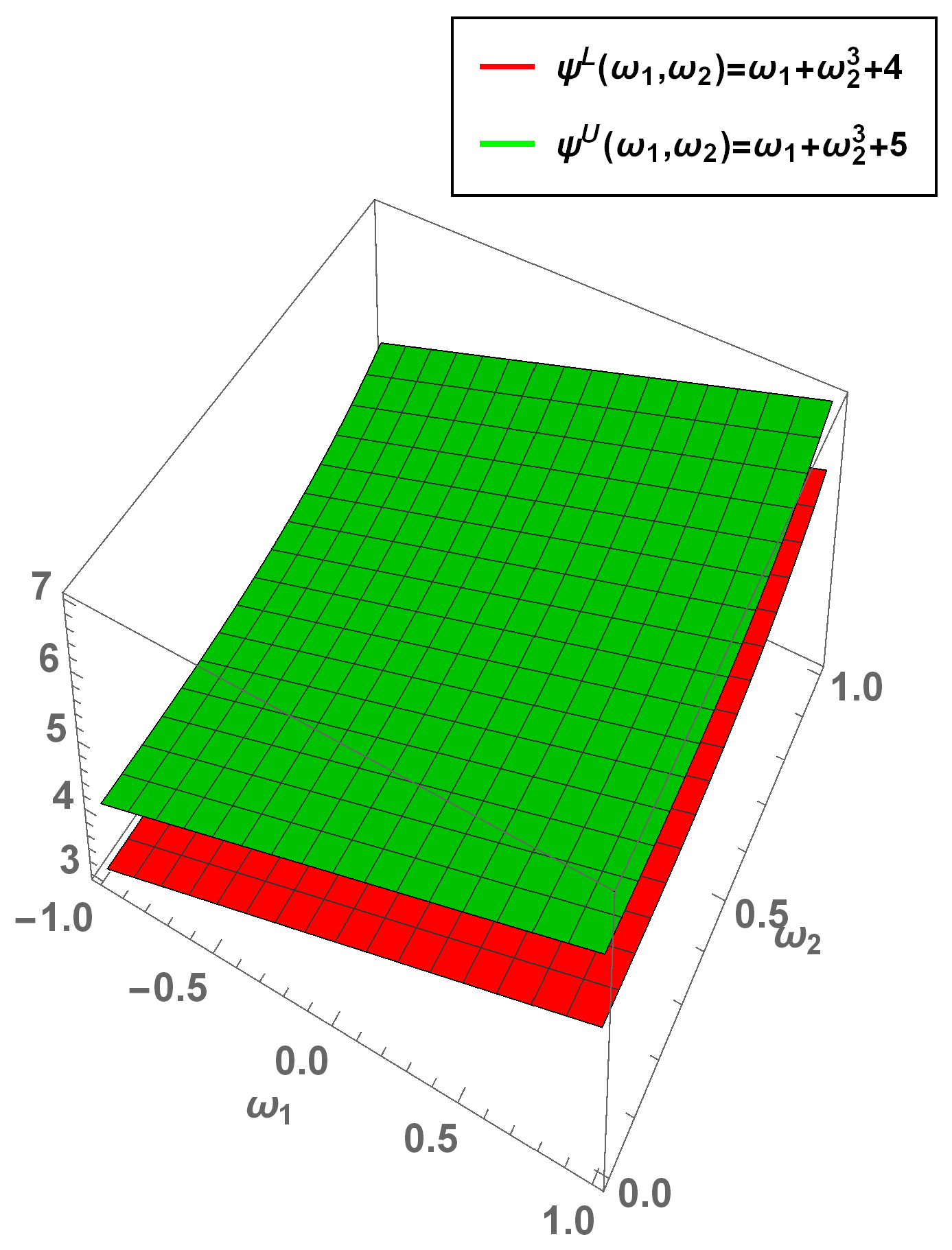
Clearly, $({\Psi }^{\mathcal{L}},{\Psi }^{\mathcal{U}},\phi )$ is type I and type II $(\mathcal{C},\mathcal{C},{\mathcal{R}}_{+}^{m_0})$-pseudo convex at ${\varpi }_0$ (See Figure 2). It follows from Example 1, we have $({\vartheta }_1,{\vartheta }_2,\varrho ,{\mu }^{\mathcal{L}},{\mu }^{\mathcal{U}},\gamma )\in {\mathbb{H}}_D^{MW}$ where ${\mu }^{\mathcal{L}}=1/2={\mu }^{\mathcal{U}}$, $\gamma ={(1/4,1)}^T\in {\mathcal{R}}_{+}^2$, $\varrho =0\in \Phi$. For any $({\varpi }_1,{\varpi }_2,\varrho ,{\mu }^{\mathcal{L}},{\mu }^{\mathcal{U}},\gamma )\in {\mathbb{H}}_D^{MW}$, ${\mu }^{\mathcal{L}},{\mu }^{\mathcal{U}}\in {\mathcal{C}}^{*}\backslash \left\{0\right\}$, $\gamma =({\gamma }_1$, ${\gamma }_2{)}^T\in {\mathcal{R}}_{+}^2$, we get

$$\left(\begin{array}{c}0\\ \\ 0\end{array}\right)=\left(\begin{array}{c}1\\ \\ 3{\varpi }_2^2\end{array}\right){\mu }^{\mathcal{L}}+\left(\begin{array}{c}1\\ \\ 3{\varpi }_2^2\end{array}\right){\mu }^{\mathcal{U}}+\left(\begin{array}{cc}2{\varpi }_1-2& 0\\ 0& -1\end{array}\right)\left(\begin{array}{c}{\gamma }_1\\ \\ {\gamma }_2\end{array}\right)$$

The above equation yields ${\mu }^{\mathcal{L}}+{\mu }^{\mathcal{U}}+2({\varpi }_1-1){\gamma }_1=0$ and $3{\varpi }_2^2({\mu }^{\mathcal{L}}+{\mu }^{\mathcal{U}})-{\gamma }_2=0$. Combining these equations along with ${\mu }^{\mathcal{L}},{\mu }^{\mathcal{U}},{\gamma }_1,{\gamma }_2\ge 0$, we obtain ${\varpi }_2\ge 0$. Since, ${\gamma }^T\phi ({\varpi }_0,\varrho )\ge 0$, that is,

$$\left(\begin{array}{cc}{\gamma }_1& {\gamma }_2\end{array}\right)\left(\begin{array}{c}{\varpi }_1^2-2{\varpi }_1-3+ln(1+{\varrho }_1)\\ \\ -{\varpi }_2-\left|{\varrho }_2\right|\end{array}\right)\ge 0.$$

This implies,

$${\gamma }_1[{\varpi }_1^2-2{\varpi }_1-3+ln(1+{\varrho }_1)]+{\gamma }_1[-{\varpi }_2-|{\varrho }_2\left|\right]\ge 0.$$

Since ${\gamma }_1\ge 0$ and $-{\varpi }_2-\left|{\varrho }_2\right|\le 0$, we have

$${\varpi }_1^2-2{\varpi }_1-3+ln(1+{\varrho }_1)\ge 0.$$

This implies, ${\varpi }_1\le -1$ for ${\varrho }_1=0$. Taking into account ${\varpi }_2\ge 0$, ${\varpi }_1\le -1$ and $\forall ({\varpi }_1,{\varpi }_2,\varrho ,{\mu }^{\mathcal{L}},{\mu }^{\mathcal{U}},\gamma )\in {\mathbb{H}}_D^{MW}$, we get,

$${\mu }^{\mathcal{L}}[{\Psi }^{\mathcal{L}}({\vartheta }_1,{\vartheta }_2)-{\Psi }^{\mathcal{L}}({\varpi }_1,{\varpi }_2)]+{\mu }^{\mathcal{U}}[{\Psi }^U({\vartheta }_1,{\vartheta }_2)-{\Psi }^{\mathcal{U}}({\varpi }_1,{\varpi }_2)]=-1-{\varpi }_1-{\varpi }_2^3\nless 0.$$

Therefore, weak duality theorem of (MWIVRD-2) holds.

Theorem 8

(Strong Duality). Let ${\overline{\vartheta }}_0$ be a robust $\mathcal{LU}$-optimal solution of (UCIVOP) and (GRSCQ) hold. Assume that φ satisfy the Assumption $\mathbb{D}$, ϕ is ${\mathcal{R}}_{+}$ - convexlike and ${\Psi }^{\mathcal{L}}$, ${\Psi }^{\mathcal{U}}$ be $\mathcal{C}$-convexlike. Then, there exist $\overline{\varrho }\in \Phi$, ${\overline{\mu }}^{\mathcal{L}},{\overline{\mu }}^{\mathcal{U}}\in {\mathcal{C}}^{*}\backslash \left\{0\right\}$, $\overline{\gamma }\in {\mathcal{R}}_{+}^{m_0}$ such that $({\overline{\vartheta }}_0,\overline{\varrho },{\overline{\mu }}^{\mathcal{L}},{\overline{\mu }}^U,\overline{\gamma })\in {\mathbb{H}}_D^{MW}$.

(i).

If $({\Psi }^{\mathcal{L}},{\Psi }^{\mathcal{U}},\phi )$ is type I $(\mathcal{C},\mathcal{C},{\mathcal{R}}_{+}^{m_0})$-pseudo convex at ${\varpi }_0$ where $({\varpi }_0,\varrho ,{\mu }^{\mathcal{L}},{\mu }^{\mathcal{U}},\gamma )\in {\mathbb{H}}_D^{MW}$, then $({\overline{\vartheta }}_0,\overline{\varrho },{\overline{\mu }}^{\mathcal{L}},{\overline{\mu }}^{\mathcal{U}},\overline{\gamma })$ is a robust $\mathcal{LU}$-optimal solution of (MWIVRD).

(ii).

If $({\Psi }^{\mathcal{L}},{\Psi }^{\mathcal{U}},\phi )$ is type II $(\mathcal{C},\mathcal{C},{\mathcal{R}}_{+}^{m_0})$-pseudo convex at ${\varpi }_0$ where $({\varpi }_0,\varrho ,{\mu }^{\mathcal{L}},{\mu }^{\mathcal{U}},\gamma )\in {\mathbb{H}}_D^{MW}$, then $({\overline{\vartheta }}_0,\overline{\varrho },{\overline{\mu }}^{\mathcal{L}},{\overline{\mu }}^{\mathcal{U}},\overline{\gamma })$ is a robust $\mathcal{LU}$-optimal solution of (MWIVRD).

Proof. 

Let ${\overline{\vartheta }}_0$ be a robust $\mathcal{LU}$-optimal solution of (UCIVOP) and (GRSCQ) hold. Then by Theorem 1, there exist $\overline{\varrho }\in \Phi$, ${\overline{\mu }}^{\mathcal{L}},{\overline{\mu }}^{\mathcal{U}}\in {\mathcal{C}}^{*}\backslash \left\{0\right\}$, $\overline{\gamma }\in {\mathcal{R}}_{+}^{m_0}$ such that $({\overline{\vartheta }}_0,\overline{\varrho },{\overline{\mu }}^{\mathcal{L}},{\overline{\mu }}^{\mathcal{U}},\overline{\gamma })$ satisfies

$$\begin{array}{cc}\hfill & 0\in \left\{\partial {\Psi }^{\mathcal{L}}{\left({\overline{\vartheta }}_0\right)}^T{\overline{\mu }}^{\mathcal{L}}+\partial {\Psi }^{\mathcal{U}}{\left({\overline{\vartheta }}_0\right)}^T{\overline{\mu }}^{\mathcal{U}}+{\partial }_{{\vartheta }_0}\phi ({{\overline{\vartheta }}_0,\overline{\varrho })}^T\overline{\gamma }\right\},\hfill \\ \hfill & {\overline{\gamma }}^T\phi ({\overline{\vartheta }}_0,\overline{\varrho })=0.\hfill \end{array}$$

Hence, $({\overline{\vartheta }}_0,\overline{\varrho },{\overline{\mu }}^{\mathcal{L}},{\overline{\mu }}^{\mathcal{U}},\overline{\gamma })\in {\mathbb{H}}_D^{MW}$.

To prove (i).

As $({\Psi }^{\mathcal{L}},{\Psi }^{\mathcal{U}},\phi )$ is type I pseudo convex at ${\varpi }_0$ and utilizing the assumption (i) of Theorem 7, we get that the subsequent inequality does not hold:

$$\Psi \left({\overline{\vartheta }}_0\right){<}_{\mathcal{LU}}\Psi \left({\varpi }_0\right),\forall ({\varpi }_0,\varrho ,{\mu }^{\mathcal{L}},{\mu }^{\mathcal{U}},\gamma )\in {\mathbb{H}}_D^{MW},$$

which implies that $({\overline{\vartheta }}_0,\overline{\varrho },{\overline{\mu }}^{\mathcal{L}},{\overline{\mu }}^{\mathcal{U}},\overline{\gamma })$ is a robust $\mathcal{LU}$-optimal solution of (MWIVRD).

(ii). As $({\Psi }^{\mathcal{L}},{\Psi }^{\mathcal{U}},\phi )$ is type II pseudo convex at any ${\varpi }_0$ and utilizing the assumption (ii) of Theorem 7, we get that the subsequent inequality cannot hold:

$$\Psi \left({\overline{\vartheta }}_0\right){<}_{\mathcal{LU}}\Psi \left({\varpi }_0\right),\forall ({\varpi }_0,\varrho ,{\mu }^{\mathcal{L}},{\mu }^{\mathcal{U}},\gamma )\in {\mathbb{H}}_D^{MW},$$

which implies that $({\overline{\vartheta }}_0,\overline{\varrho },{\overline{\mu }}^{\mathcal{L}},{\overline{\mu }}^{\mathcal{U}},\overline{\gamma })$ is a robust $\mathcal{LU}$-optimal solution of (MWIVRD). □

Theorem 9

(Converse Duality). Let $({\overline{\varpi }}_0,\overline{\varrho },{\overline{\mu }}^{\mathcal{L}},{\overline{\mu }}^{\mathcal{U}},\overline{\gamma })$ be a robust $\mathcal{LU}$-optimal solution of (MWIVRD) with ${\overline{\varpi }}_0\in \mathbb{H}$.

(i).

If $({\Psi }^{\mathcal{L}},{\Psi }^{\mathcal{U}},\phi )$ is type I $(\mathcal{C},\mathcal{C},{\mathcal{R}}_{+}^{m_0})$-pseudo convex at ${\overline{\varpi }}_0$, then ${\overline{\varpi }}_0$ is a robust $\mathcal{LU}$-optimal solution of (UCIVOP).

(ii).

If $({\Psi }^{\mathcal{L}},{\Psi }^{\mathcal{U}},\phi )$ is type II $(\mathcal{C},\mathcal{C},{\mathcal{R}}_{+}^{m_0})$-pseudo convex at ${\overline{\varpi }}_0$, then ${\overline{\varpi }}_0$ is a robust $\mathcal{LU}$-optimal solution of (UCIVOP).

Proof. 

To prove (i).

Since $({\overline{\varpi }}_0,\overline{\varrho },{\overline{\mu }}^{\mathcal{L}},{\overline{\mu }}^{\mathcal{U}},\overline{\gamma })$ is a robust $\mathcal{LU}$-optimal solution of (MWIVRD) with ${\overline{\varpi }}_0\in \mathbb{H}$. As $({\Psi }^{\mathcal{L}},{\Psi }^{\mathcal{U}},\phi )$ is type I pseudo convex at ${\overline{\varpi }}_0$ and utilizing the assumption (i) of Theorem 7, the subsequent inequality does not hold:

$$\Psi \left({\vartheta }_0\right){<}_{\mathcal{LU}}\Psi \left({\overline{\varpi }}_0\right),\forall {\vartheta }_0\in \mathbb{H}.$$

Hence, ${\overline{\varpi }}_0$ is a robust $\mathcal{LU}$-optimal solution of (UCIVOP).

(ii) As $({\Psi }^{\mathcal{L}},{\Psi }^{\mathcal{U}},\phi )$ is type II pseudo convex at any ${\overline{\varpi }}_0$ and utilizing the assumption (ii) of Theorem 7, the subsequent inequality cannot hold:

$$\Psi \left({\vartheta }_0\right){<}_{\mathcal{LU}}\Psi \left({\overline{\varpi }}_0\right),\forall {\vartheta }_0\in \mathbb{H}.$$

Hence, ${\overline{\varpi }}_0$ is a robust $\mathcal{LU}$-optimal solution of (UCIVOP). □

6. Conclusions

This paper uses the $\mathcal{LU}$-optimal solution and the generalized robust Slater constraint qualifications (GRSCQ) to formulate Karush- Kuhn-Tucker type robust necessary optimality conditions for an uncertain constrained interval-valued optimization problem (UCIVOP). These Karush-Kuhn-Tucker type robust necessary conditions are shown to be sufficient optimality conditions under generalized convexity. An illustration is provided to demonstrate the robust sufficient optimality theorem’s validity. Further to that, Karush-Kuhn-Tucker robust necessary conditions are used to formulate Wolfe and Mond-Weir type robust dual problems over cones. The validity of Wolfe and Mond-Weir’s weak duality theorems is demonstrated. Finally, the usual duality results are demonstrated using the generalized convexity assumptions. It would be interesting to see if these results could be obtained for other types of nonconvex vector optimization problems with multiple interval-valued objective functions, as well as other types of extremum problems. As a result, we are generalizing our current results to multiple interval-valued optimization problems with uncertainty, which we will focus on in our future research.

References

- Soyster, A.L. Convex programming with set-inclusive constraints and applications to inexact linear programming. Oper. Res. 1973, 21, 1154–1157. [Google Scholar] [CrossRef] [Green Version]
- Taguchi, G.; Chowdhury, S.; Taguchi, S. Robust Engineering; McGraw-Hill: New York, NY, USA, 2000. [Google Scholar]
- Bokrantz, R.; Fredriksson, A. Necessary and sufficient conditions for pareto efficiency in robust multi-objective optimization. Eur. J. Oper. Res. 2017, 262, 682–692. [Google Scholar] [CrossRef] [Green Version]
- Deb, K.; Gupta, H. Introducing robustness in multi-objective optimization. Evol. Comput. 2006, 14, 463–494. [Google Scholar] [CrossRef] [PubMed]
- Ide, J.; Köbis, E. Concepts of efficiency for uncertain multi-objective optimization problems based on set order relations. Math. Methods Oper. Res. 2014, 80, 99–127. [Google Scholar] [CrossRef]
- Ide, J.; Schöbel, A. Robustness for uncertain multi-objective optimization: A survey and analysis of different concepts. OR Spectr. 2016, 38, 235–271. [Google Scholar] [CrossRef]
- Syberfeldt, A.; Gustavsson, P. Increased robustness of product sequencing using multi-objective optimization. Procedia CIRP 2014, 17, 434–439. [Google Scholar] [CrossRef]
- Wiecek, M.M.; Dranichak, G.M. Robust multi-objective optimization for decision making under uncertainty and conflict. In Optimization Challenges in Complex, Networked and Risky Systems; INFORMS: Catonsville, MD, USA, 2016; pp. 84–114. [Google Scholar]
- Lee, J.; Wu, F.; Zhao, W.; Ghaffari, M.; Liao, L.; Siegel, D. Prognostics and health management design for rotary machinery systems-Reviews, methodology and applications. Mech. Syst. Signal Process. 2014, 42, 314–334. [Google Scholar] [CrossRef]
- Oksanen, T.; Linkolehto, R.; Seilonen, I. Adapting an industrial automation protocol to remote monitoring of mobile agricultural machinery: A combine harvester with IoT. IFAC-PapersOnLine 2016, 49, 127–131. [Google Scholar] [CrossRef]
- Lei, G.; Bramerdorfer, G.; Ma, B.; Guo, Y.; Zhu, J. Robust design optimization of electrical machines: Multi-objective approach. IEEE Trans. Energy Convers. 2020, 36, 390–401. [Google Scholar] [CrossRef]
- Ahmadi-Nezamabad, H.; Zand, M.; Alizadeh, A.; Vosoogh, M.; Nojavan, S. Multi-objective optimization based robust scheduling of electric vehicles aggregator. Sustain. Cities Soc. 2019, 47, 101494. [Google Scholar] [CrossRef]
- Doolittle, E.K.; Kerivin, H.L.M.; Wiecek, M.M. Robust multi-objective optimization problem with application to internet routing. Ann. Oper. Res. 2018, 271, 487–525. [Google Scholar] [CrossRef]
- Krüger, C.; Castellani, F.; Geldermann, J.; Schöbel, A. Peat and pots: An application of robust multi-objective optimization to a mixing problem in agriculture. Comput. Electron. Agric. 2018, 154, 265–275. [Google Scholar] [CrossRef]
- Palma, C.D.; Nelson, J.D. Bi-objective multi-period planning with uncertain weights: A robust optimization approach. Eur. J. For. Res. 2010, 129, 1081–1091. [Google Scholar] [CrossRef]
- Ahmad, I.; Kummari, K.; Al-Homidan, S. Sufficiency and duality for interval-valued optimization problems with vanishing constraints using weak constraint qualifications. Int. J. Anal. Appl. 2020, 18, 784–798. [Google Scholar]
- Kummari, K.; Ahmad, I. Sufficient optimality conditions and duality for nonsmooth interval-valued optimization problems via L-invex-infine functions. Politehn. Univ. Buchar. Sci. Bull. Ser. A Appl. Math. Phys. 2020, 82, 45–54. [Google Scholar]
- Singh, D.; Dar, B.; Goyal, A. KKT optimality conditions for interval-valued optimization problems. J. Nonlinear Anal. Optim. Theory Appl. 2014, 5, 91–103. [Google Scholar]
- Zhang, J.; Zheng, Q.; Zhou, C.; Ma, X.; Li, L. On interval-valued pseudo-linear functions and interval-valued pseudo-linear optimization problems. J. Funct. Spaces 2015, 2015, 610848. [Google Scholar]
- Zhao, J.; Bin, M. Karush-Kuhn-Tucker optimality conditions for a class of robust optimization problems with an interval-valued objective function. Open Math. 2020, 18, 781–793. [Google Scholar] [CrossRef]
- Shaikh, A.A.; Das, S.C.; Bhunia, A.K.; Panda, G.C.; Khan, M.A.A. A two-warehouse EOQ model with interval-valued inventory cost and advance payment for deteriorating item under particle swarm optimization. Soft Comput. 2019, 23, 13531–13546. [Google Scholar] [CrossRef]
- Wang, W.; Xiong, J.; Xie, M. A study of interval analysis for cold-standby system reliability optimization under parameter uncertainty. Comput. Ind. Eng. 2016, 97, 93–100. [Google Scholar] [CrossRef]
- Zhang, Z.; Wang, X.; Lu, J. Multi-objective immune genetic algorithm solving nonlinear interval-valued programming. Eng. Appl. Artif. Intell. 2018, 67, 235–245. [Google Scholar] [CrossRef]
- Arrow, K.J.; Enthoven, A.C. Quasi-concave programming. Econometrica 1961, 779–800. [Google Scholar] [CrossRef]
- Hanson, M.A. On sufficiency of the Kuhn-Tucker conditions. J. Math. Anal. Appl. 1981, 80, 545–550. [Google Scholar] [CrossRef] [Green Version]
- Craven, B.D. Invex functions and constrained local minima. Bull. Aust. Math. Soc. 1981, 24, 357–366. [Google Scholar] [CrossRef] [Green Version]
- De Carvalho Bento, G.; Bitar, S.D.B.; da Cruz Neto, J.X.; Soubeyran, A.; de Oliveira Souza, J.C. A proximal point method for difference of convex functions in multi-objective optimization with application to group dynamic problems. Comput. Optim. Appl. 2020, 75, 263–290. [Google Scholar] [CrossRef]
- Fakhar, M.; Mahyarinia, M.R.; Zafarani, J. On nonsmooth robust multi-objective optimization under generalized convexity with applications to portfolio optimization. Eur. J. Oper. Res. 2018, 265, 39–48. [Google Scholar] [CrossRef]
- Günther, C. On Generalized Convex Constrained Multi-Objective Optimization and Application in Location Theory; University and State Library of Saxony-Anhalt: Halle, Germany, 2018. [Google Scholar]
- Suneja, S.K.; Khurana, S.; Bhatia, M. Optimality and duality in vector optimization involving generalized type I functions over cones. J. Glob. Optim. 2011, 49, 23–35. [Google Scholar] [CrossRef]
- Chen, J.W.; Cho, Y.J.; Kim, J.K.; Li, J. Multi-objective optimization problems with modified objective functions and cone constraints and applications. J. Glob. Optim. 2011, 49, 137–147. [Google Scholar] [CrossRef]
- Lee, G.M.; Son, P.T. On nonsmooth optimality theorems for robust optimization problems. Bull. Korean Math. Soc. 2014, 51, 287–301. [Google Scholar] [CrossRef] [Green Version]
- Lee, G.M.; Lee, J.H. On nonsmooth optimality theorems for robust multi-objective optimization problems. J. Nonlinear Convex Anal. 2015, 16, 2039–2052. [Google Scholar]
- Chuong, T.D. Optimality and duality for robust multi-objective optimization problems. Nonlinear Anal. 2016, 134, 127–143. [Google Scholar] [CrossRef]
- Ben-Tal, A.; Ghaoui, L.E.l.; Nemirovski, A. Robust Optimization; Princeton Series in Applied Mathematics; Princeton University Press: Princeton, NJ, USA, 2009. [Google Scholar]
- Jeyakumar, V.; Li, G.Y. Strong duality in robust convex programming: Complete characterizations. SIAM J. Optim. 2010, 20, 3384–3407. [Google Scholar] [CrossRef]
- Mangasarian, O.L. Nonlinear Programming; SIAM: Philadelphia, PA, USA, 1994. [Google Scholar]
- Ishibuchi, H.; Tanaka, H. Multi-objective programming in optimization of the interval objective function. Eur. J. Oper. Res. 1990, 48, 219–225. [Google Scholar] [CrossRef]
- Inuiguchi, M.; Kume, Y. Goal programming problems with interval coefficients and target intervals. Eur. J. Oper. Res. 1991, 52, 345–360. [Google Scholar] [CrossRef]
- Wu, H.C. The Karush-Kuhn-Tucker optimality conditions in an optimization problem with interval-valued objective function. Eur. J. Oper. Res. 2007, 176, 46–59. [Google Scholar] [CrossRef]
- Wu, H.C. The Karush-Kuhn-Tucker optimality conditions in multi-objective programming problems with interval-valued objective functions. Eur. J. Oper. Res. 2009, 196, 49–60. [Google Scholar] [CrossRef]
- Chen, J.; Köbis, E.; Yao, J.C. Optimality conditions and duality for robust nonsmooth multi-objective optimization problems with constraints. J. Optim. Theory Appl. 2019, 181, 411–436. [Google Scholar] [CrossRef]
- Clarke, F.H. Optimization and Nonsmooth Analysis; Society for Industrial and Applied Mathematics: Philadelphia, PA, USA, 1990. [Google Scholar]
- Saadati, M.; Oveisiha, M. Optimality conditions for robust nonsmooth multi-objective optimization problems in Asplund spaces. arXiv 2021, arXiv:2105.14366. [Google Scholar]
- Singh, D.; Dar, B.A.; Kim, D.S. Sufficiency and duality in non-smooth interval valued programming problems. J. Ind. Manag. Optim. 2019, 15, 647–665. [Google Scholar] [CrossRef] [Green Version]
Figure 1.
Graphical view of the objective functions and of the problem (UCIVOP-1).
Figure 2.
Graphical view of the objective functions and of the problem (MWIVRD-2).
Publisher’s Note: MDPI stays neutral with regard to jurisdictional claims in published maps and institutional affiliations. |
© 2022 by the authors. Licensee MDPI, Basel, Switzerland. This article is an open access article distributed under the terms and conditions of the Creative Commons Attribution (CC BY) license (https://creativecommons.org/licenses/by/4.0/).
Share and Cite
MDPI and ACS Style
Jaichander, R.R.; Ahmad, I.; Kummari, K.; Al-Homidan, S. Robust Nonsmooth Interval-Valued Optimization Problems Involving Uncertainty Constraints. Mathematics 2022, 10, 1787. https://0-doi-org.brum.beds.ac.uk/10.3390/math10111787
AMA Style
Jaichander RR, Ahmad I, Kummari K, Al-Homidan S. Robust Nonsmooth Interval-Valued Optimization Problems Involving Uncertainty Constraints. Mathematics. 2022; 10(11):1787. https://0-doi-org.brum.beds.ac.uk/10.3390/math10111787
Chicago/Turabian StyleJaichander, Rekha R., Izhar Ahmad, Krishna Kummari, and Suliman Al-Homidan. 2022. "Robust Nonsmooth Interval-Valued Optimization Problems Involving Uncertainty Constraints" Mathematics 10, no. 11: 1787. https://0-doi-org.brum.beds.ac.uk/10.3390/math10111787
Note that from the first issue of 2016, this journal uses article numbers instead of page numbers. See further details here.