Article

Queueing-Inventory System for Two Commodities with Optional Demands of Customers and MAP Arrivals

1
Department of Mathematics, Alagappa University, Karaikudi 630003, India
2
Department of Computer Science and Engineering, Sejong University, Seoul 05006, Korea
3
Ramanujan Center for Higher Mathematics, Alagappa University, Karaikudi 630003, India
4
Department of Electronic Engineering, Kwangwoon University, Seoul 01897, Korea
*
Authors to whom correspondence should be addressed.
These authors contributed equally to this work.
Submission received: 24 April 2022 / Revised: 20 May 2022 / Accepted: 22 May 2022 / Published: 25 May 2022
(This article belongs to the Special Issue Mathematical Modelling and Optimization of Service Supply Chain)

Abstract

:
This research analyses the performance of a perishable queueing-inventory system for two commodities with optional customers demands. We assume in the article that all customers who come to the system can only purchase the first item or the second item or service (they do not purchase both items). This is the original aspect of the paper. We show the significance of the impact of optional demands on the system’s performance, which is the purpose of the paper. In this system, customers arrive, using the Markovian arrival process (MAP), to a demand for a single unit. The system is composed of a waiting hall with a limited capacity of F. The arriving customer observes the waiting hall is filled to capacity or the stock stage is zero, and they decide to leave the system. In the steady-state case, the joint probability distribution for the first commodity, the second commodity, and the number of customers in the system are computed using matrix geometric methods. We evaluate diverse system performance measures. Finally, we provide a numerical illustration of the optimal value for diverse parameters of the system, which highlights the results and implications of the article.

1. Introduction

One of the critical problems in an inventory system is having a large number of items which can affect its integrated functioning. To avoid this problem, multiple commodity systems are used. To manage such systems numerous models have been proposed with various sorts of ordering policies. The joint ordering policy was introduced by [1] and developed by [2]. A two commodity inventory system with zero lead time and with the same demand process were inspected by [3,4], respectively. The authors of [5,6] analyzed a joint ordering policy with a substitutable inventory system. A queueing-inventory system can be manipulated according to a number of factors, such as arrival/service processes, waiting hall capacity, service interruption, and vacation assumptions. See [7,8] review articles and [9,10,11,12,13,14,15,16,17,18,19] articles for discussion of a two commodity queueing-inventory system.
A system needs to satisfy different kinds of customer demands to achieve profit. Sometimes customers need only service without purchasing an item. For example, in a mechanic shop, customers may come to repair their vehicle. Some customers come to the system with a required item—they only need service. Some customers come to the system without items—they need service with the item. In a similar way, we can observe this sort of circumstance in a tailoring shop, card printers, etc. In this circumstance, the system provides the same services for both demands.
Motivated by practical situations that arise, we consider how arriving customers may choose either service with or without an item. The present article also considers a perishable ( s , Q ) queueing-inventory system for two commodities in which customers arrive according to a Markovian arrival process (MAP) to a single unit or for service at a certain time.
A MAP is a type of tractable class of the Markov renewal process. The arrival process can be modified to be a renewal process by adjusting the MAP’s parameters. The MAP is a diverse class of point processes that also includes the Poisson process. The purpose of MAP is to generalize the Poisson process and create more flexibility for modeling purposes. MAP may be used for both discrete and continuous time frames, but this paper focuses only on continuous-time frames. An explanation of MAP is provided by [20]. The states of the Markov chain are 1 , 2 , y . When the chain goes into the state u, 1 u y , it remains with parameter m u for an exponential time. When the sojourn period is over, the chain may shift to a transition until arrival occurs; then the chain goes into the state v with the probability c u v , 1 v y , or if transition occurs without arrival, then the chain goes into the state v with probability d u v , 1 v y , u v . When an arrival occurs, the chain might return to the same state. We describe the square matrices D f , f = 0 , 1 , of size y by D 0 u u = m u and D 0 u v = m u d u v , u v , D 1 u v = m u c u v , 1 u , v y . χ represents the continuous time Markov chain’s unique probability vector with an infinitesimal generator matrix D ( = D 0 + D 1 ) , and χ is obtained from χ D = 0 , χ e = 1 .
Let φ represent the initial probability vector of the underlying MAP-based Markov process. We have an independent arrival, the end of an interval with minimum k arrivals, and the moment at which the system enters or exits a certain state, such as when a busy period begins or ends, etc.; by choosing a suitable φ , we can obtain the kind of time. The main purpose is that we obtain the unique probability vector of MAP by φ = χ . The average arrival rate λ = χ D 1 e provides the mean number of customers occurring per unit time. The MAP-described point process is a special category of semi-Markov processes with a transition probability matrix provided by
0 x e D 0 t d t D 1 = [ I e D 0 x ] ( D 0 ) 1 D 1 , x 0 .
For more information on MAP, readers can refer to [21,22,23]. Table 1 summarizes the overview of literature review.
The findings of the above survey inspired our research, since, to our knowledge, there has been little study into two commodities with three forms of service, which is a common occurrence in business administration. Section 2 discusses the detailed description of our model. In Section 3, we provide an analysis of our prescriptive model. Analysis of the model’s steady-state is described in Section 4. In Section 5, we develop several aspects of system performance for the steady-state case. In Section 6, the total expected cost rate (TCR) is calculated. In Section 7, numerical examples are provided.

2. Model Narrations

A two-commodity perishable queueing-inventory system is considered. The system has a maximum capacity of S 1 items for the first commodity, and S 2 items for the second commodity. The system provides the finite waiting room size of F along with one getting service. The customers show up as per MAP, with demand for a single unit. A single item of the first commodity is required by the customer (i.e., a high quality and high price item) with probability b 1 or the second commodity (i.e., a normal quality and cheap price item) with probability b 2 or service only with probability b 3 . The server’s service is the same for each demand. With parameter b i μ , ( i = 1 , 2 , 3 ) , three different kinds of service times are exponentially distributed. We take the parameter γ 1 as the lifetime of the first commodity and γ 2 for the second commodity follows an exponential distribution. If both stock levels are close to their respective reorder levels s i i = 1 , 2 , then an order is made for both commodities. Q i > s i , i = 1 , 2 units are considered the ordering quantity for the i-th commodity. The lead time follows an exponential distribution with parameter β ( > 0 ) . The customer arrives during a stock-out period and the full system is considered to be lost. Customers leave the system after receiving the required service performances of the item.

3. Analysis

We consider I ( 1 ) ( t ) to represent the number of items in the first commodity at time t, I ( 2 ) ( t ) to represent the number of items in the second commodity at time t, N ( t ) to represent the number of customers in the system at time t and J ( t ) to represent the phase of the arrival process at time t. The Markov process I ( 1 ) ( t ) , I ( 2 ) ( t ) , N ( t ) , J ( t ) ; t 0 with discrete state space E = E 1 × E 2 × E 3 × E 4 , where 0 E 1 S 1 , 0 E 2 S 2 , 0 E 3 F , 1 E 4 y . The infinitesimal generator matrix W i j = O i , j = i × 1 ,   i = 1 , 2 , S 1 P i , j = i ,   i = 0 , 1 , S 1 R , j = i + Q 1 ,   i = 0 , 1 , s 1 0 , otherwise where R k l = β I Z I y , l = k + Q 2 ,   k = 0 , 1 , s 2 , 0 , otherwise . where, Z = F + 1
Here, i = 1 , 2 , S 1 and A Z = [ a i j ] Z × Z = 1 , if j = i 1 , i = 1 , 2 , F 0 , otherwise
O i k l = i γ 1 I Z + b 1 μ A Z I y , l = k , k = 0 , 1 , S 2 , 0 , otherwise .
Here, B Z = [ b i j ] Z × Z = 1 , if j = i + 1 , i = 0 , 1 , F 1 0 , otherwise
C Z = [ c i j ] Z × Z = 1 , if j = i , i = F 0 , otherwise
G Z = [ g i j ] Z × Z = 1 , if j = i , i = 0 , 1 , F 1 0 , otherwise
H Z = [ h i j ] Z × Z = 1 , if j = i , i = 1 , 2 , F 0 , otherwise
For i = 0 ,
P i k l = k γ 2 I Z + b 2 μ A Z I y , l = k 1 , k = 1 , 2 , S 2 , b 3 μ A Z I y + B Z D 1 + ( G Z D 0 + C Z D I Z β I y + H Z ( b 3 μ ) I y ) , l = k , k = 0 , b 3 μ A Z I y + B Z D 1 + ( G Z D 0 + C Z D I Z β + k γ 2 I y + H Z ( b 3 μ + b 2 μ ) I y ) , l = k , k = 1 , 2 , s 2 , b 3 μ A Z I y + B Z D 1 + ( G Z D 0 + C Z D I Z k γ 2 I y + H Z ( b 3 μ + b 2 μ ) I y ) , l = k , k = s 2 + 1 , s 2 + 2 , S 2 , 0 , otherwise .
For i = 1 , 2 , s 1 ,
P i k l = k γ 2 I Z + b 2 μ A Z I y , l = k 1 , k = 1 , 2 , S 2 , b 3 μ A Z I y + B Z D 1 + ( G Z D 0 + C Z D I Z β + i γ 1 I y + H Z ( b 3 μ + b 1 μ ) I y ) , l = k , k = 0 , b 3 μ A Z I y + B Z D 1 + ( G Z D 0 + C Z D I Z β + i γ 1 + k γ 2 I y + H Z ( b 3 μ + b 1 μ + b 2 μ ) I y ) , l = k , k = 1 , 2 , s 2 , b 3 μ A Z I y + B Z D 1 + ( G Z D 0 + C Z D I Z i γ 1 + k γ 2 I y + H Z ( b 3 μ + b 1 μ + b 2 μ ) I y ) , l = k , k = s 2 + 1 , S 2 , 0 , otherwise .
For i = s 1 + 1 , S 1 ,
P i k l = k γ 2 I Z + b 2 μ A Z I y , l = k 1 , k = 1 , 2 , S 2 , b 3 μ A Z I y + B Z D 1 + ( G Z D 0 + C Z D         I Z i γ 1 I y + H Z ( b 3 μ + b 1 μ ) I y ) , l = k , k = 0 , b 3 μ A Z I y + B Z D 1 + ( G Z D 0 + C Z D         I Z i γ 1 + k γ 2 I y + H Z ( b 3 μ + b 1 μ + b 2 μ ) I y ) , l = k , k = 1 , 2 , S 2 , 0 , otherwise .

4. Steady State Analysis

From the structure of W , the Markov process I ( 1 ) ( t ) , I ( 2 ) ( t ) , N ( t ) , J ( t ) ; t 0 on the state space E is irreducible, and the limiting distribution Y ( i 1 , i 2 , i 3 , i 4 ) = lim t P r [ I ( 1 ) ( t ) = i 1 , I ( 2 ) ( t ) = i 2 , N ( t ) = i 3 , J ( t ) = i 4 ; I ( 1 ) ( 0 ) , I ( 2 ) ( 0 ) , N ( 0 ) , J ( 0 ) ] , exists.
The limiting distribution Y ( i 1 , i 2 , i 3 , i 4 ) is independent of the starting condition.
Take
Y = ( Y ( 0 ) , Y ( 1 ) , , Y ( S 1 ) ) , where   Y ( i 1 ) = ( Y ( i 1 , 0 ) , Y ( i 1 , 1 ) , , Y ( i 1 , S 2 ) ) , i 1 = 0 , 1 , , S 1 Y ( i 1 , i 2 ) = ( Y ( i 1 , i 2 , 0 ) , Y ( i 1 , i 2 , 1 ) , , Y ( i 1 , i 2 , F ) ) , i 2 = 0 , 1 , , S 2 Y ( i 1 , i 2 , i 3 ) = ( Y ( i 1 , i 2 , i 3 , 1 ) , Y ( i 1 , i 2 , i 3 , 2 ) , , Y ( i 1 , i 2 , i 3 , y ) ) , i 3 = 0 , 1 , , F
The steady-state probability vector Y obtained from Y W = 0, Y e = 1.
Theorem 1.
The steady-state probability vector Y for the Markov process whose rate matrix W is given by
Y ( i 1 ) = Y ( Q 1 ) Ω i 1 ,         i 1 = 0 , 1 , , S 1
where
Ω i 1 = ( 1 ) Q 1 i 1 O Q 1 P Q 1 1 1 O Q 1 1 O i 1 + 1 P i 1 1 , i 1 = 0 , 1 , Q 1 1 ; I , i 1 = Q 1 ; ( 1 ) 2 Q 1 i 1 + 1 j = 0 S 1 i 1 ( O Q 1 P Q 1 1 1 O Q 1 1 O s 1 + 1 j P s 1 j 1 ) R P S 1 j 1 ( O S 1 j P S 1 j 1 1 O S 1 j 1 O i 1 + 1 P i 1 1 ) , i 1 = Q 1 + 1 , , S 1 ;
The following two equations can be used to arrive to Y ( Q 1 ) :
( i . e ) Y ( Q 1 ) ( ( 1 ) Q 1 j = 0 s 1 1 ( O Q 1 P Q 1 1 1 O Q 1 1 O s 1 + 1 j P s 1 j 1 ) R P S 1 j 1 ( O S 1 j P S 1 j 1 1 O S 1 j 1 O Q 1 + 2 P Q 1 + 1 1 ) O Q 1 + 1 + P Q 1 + ( 1 ) Q 1 O Q 1 P Q 1 1 1 O Q 1 1 O 1 P 0 1 R ) = 0
and
Y ( Q 1 ) ( i 1 = o Q 1 1 ( 1 ) Q 1 i 1 O Q 1 P Q 1 1 1 O Q 1 1 O i 1 + 1 P i 1 1 + I + i 1 = Q 1 + 1 S 1 { ( 1 ) 2 Q 1 i 1 + 1 j = 0 S 1 i 1 { ( O Q 1 P Q 1 1 1 O Q 1 1 O s 1 + 1 j P s 1 j 1 ) R P S 1 j 1 ( O S 1 j P S 1 j 1 1 O S 1 j 1 O i 1 + 1 P i 1 1 ) } } ) e = 1
Proof. 
We know that
Y W = 0   and   Y e = 1 .
The equation Y W = 0 can be written as
Y ( i 1 + 1 ) O i 1 + 1 + Y ( i 1 ) P i 1 = 0 , i 1 = 0 , 1 , Q 1 1 Y ( i 1 + 1 ) O i 1 + 1 + Y ( i 1 ) P i 1 + Y ( i 1 Q 1 ) R = 0 , i 1 = Q 1 Y ( i 1 + 1 ) O i 1 + 1 + Y ( i 1 ) P i 1 + Y ( i 1 Q 1 ) R = 0 , i 1 = Q 1 + 1 , Q 1 + 2 , S 1 1 Y ( i 1 ) P i 1 + Y ( i 1 Q 1 ) R = 0 , i 1 = S 1 .
The equations, except (1), can be solved recursively, yielding
Y ( i 1 ) = Y ( Q 1 ) Ω i 1 ,         i = 0 , 1 , , S 1
where
Ω i 1 = ( 1 ) Q 1 i 1 O Q 1 P Q 1 1 1 O Q 1 1 O i 1 + 1 P i 1 1 , i 1 = 0 , 1 , Q 1 1 ; I , i 1 = Q 1 ; ( 1 ) 2 Q 1 i 1 + 1 j = 0 S 1 i 1 ( O Q 1 P Q 1 1 1 O Q 1 1 O s 1 + 1 j P s 1 j 1 ) R P S 1 j 1 ( O S 1 j P S 1 j 1 1 O S 1 j 1 O i 1 + 1 P i 1 1 ) , i 1 = Q 1 + 1 , , S 1 ;
After placing the value of Ω i 1 in (1) and in the normalizing condition, we acquire Y ( Q 1 )
( i . e ) Y ( Q 1 ) ( ( 1 ) Q 1 j = 0 s 1 1 ( O Q 1 P Q 1 1 1 O Q 1 1 O s 1 + 1 j P s 1 j 1 ) R P S 1 j 1 ( O S 1 j P S 1 j 1 1 O S 1 j 1 O Q 1 + 2 P Q 1 + 1 1 ) O Q 1 + 1 + P Q 1 + ( 1 ) Q 1 O Q 1 P Q 1 1 1 O Q 1 1 O 1 P 0 1 R ) = 0
and
Y ( Q 1 ) ( i 1 = o Q 1 1 ( 1 ) Q 1 i 1 O Q 1 P Q 1 1 1 O Q 1 1 O i 1 + 1 P i 1 1 + I + i 1 = Q 1 + 1 S 1 { ( 1 ) 2 Q 1 i 1 + 1 j = 0 S 1 i 1 { ( O Q 1 P Q 1 1 1 O Q 1 1 O s 1 + 1 j P s 1 j 1 ) R P S 1 j 1 ( O S 1 j P S 1 j 1 1 O S 1 j 1 O i 1 + 1 P i 1 1 ) } } ) e = 1

5. System Performance Measures

In this division, we surmise a few performance measures in the system.

5.1. Mean Inventory Level

Let M I ( 1 ) and M I ( 2 ) be the mean inventory levels of the first and second commodities, respectively, in a steady state, which can be expressed as
M I ( 1 ) = i 1 = 1 S 1 i 1 i 2 = 0 S 2 i 3 = 0 F Y ( i 1 , i 2 , i 3 ) e
M I ( 2 ) = i 2 = 1 S 2 i 2 i 1 = 0 S 1 i 3 = 0 F Y ( i 1 , i 2 , i 3 ) e

5.2. Mean Reorder Rate

In a stable state, the M R represents the mean reorder rate. The joint inventory level decreases to ( s 1 , s 2 ) or ( s 1 , i 2 ) , i 2 < s 2 or ( i 1 , s 2 ) , i 1 < s 1 if once service is performed, or if any of the ( s i + 1 ) , i = 1 , 2 items are perishable.
M R = ( s 1 + 1 ) γ 1 i 2 = 0 s 2 i 3 = 0 F Y ( s 1 + 1 , i 2 , i 3 ) e + ( s 2 + 1 ) γ 2 i 1 = 0 s 1 i 3 = 0 F Y ( i 1 , s 2 + 1 , i 3 ) e + b 1 μ i 3 = 1 F i 2 = 0 s 2 Y ( s 1 + 1 , i 2 , i 3 ) e + b 2 μ i 3 = 1 F i 1 = 0 s 1 Y ( i 1 , s 2 + 1 , i 3 ) e .

5.3. Mean Perishable Rate

Let M P 1 and M P 2 be the mean perishable rates of the first and second commodity, respectively, in a steady state and are given by
M P 1 = i 1 = 1 S 1 i 2 = 0 S 2 i 3 = 0 F i 1 γ 1 Y ( i 1 , i 2 , i 3 ) e
M P 2 = i 1 = 0 S 1 i 2 = 1 S 2 i 3 = 0 F i 2 γ 2 Y ( i 1 , i 2 , i 3 ) e .

6. Cost Analysis

For the total expected cost function per unit time, we have evaluated the cost aspects listed below.
  • C C i : Carrying cost of i-th commodity per unit time ( i = 1 , 2 )
  • C S : Setup cost per order
  • C P 1 : First-commodity perishable cost per item per unit time
  • C P 2 : Second-commodity perishable cost per item per unit time
The total expected cost function is given by
T C ( S 1 , s 1 , S 2 , s 2 , F ) = C C 1 M I ( 1 ) + C C 2 M I ( 2 ) + C S M R + C P 1 M P 1 + C P 2 M P 2
where M I ( i ) , M R and M P i (i = 1, 2) are given in Section 5.

7. Numerical Illustration

The convexity of the TCR is demonstrated using numerical examples. We presume the below numerical example: The arrival process is hyper-exponential. As a MAP, its parameters are given by ( D 0 , D 1 ) where
D 0 = 10 0 0 1   and   D 1 = 9 1 0.9 0.1
Let F = 6, s 1 = 3 , s 2 = 2 , β = 0.45 , μ = 1.6 , γ 1 = 0.7 , γ 2 = 0.5 , b 1 = 0.4 , b 2 = 0.32 , b 3 = 0.28 ; C C 1 = 1.4 , C C 2 = 1.35 , C P 1 = 1.28 , C P 2 = 2.7 , C S = 1 ;
Furthermore, let T C ( S 1 , S 2 ) = T C ( S 1 , 3 , S 2 , 2 , 6 ) .
This gives the expected cost rate for different values of S 1 and of S 2 .
In Table 2, we present the T C ( S 1 , S 2 ) values. Here, the row minimum is represented in boldface and the column minimum is underlined. A convex function of ( S 1 , S 2 ) is T C ( S 1 , S 2 ), and the optimum at ( S 1 , S 2 ) = (21, 16).
Let S 2 = 12 , s 1 = 2 , s 2 = 1 , β = 1.4 , μ = 1.7 , γ 1 = 1.01 , γ 2 = 0.05 , b 1 = 0.4 , b 2 = 0.32 , b 3 = 0.28 ; C C 1 = 1.1 , C C 2 = 0.35 , C P 1 = 1.28 , C P 2 = 2.78 , C S = 1.76 ;
Furthermore, let T C ( S 1 , F ) = TC( S 1 , 2 , 12 , 1 , F ).
This provides the TCR for different values of S 1 and of F.
In Table 3, we present the T C ( S 1 , F ) values. Here, the row minimum is represented in boldface and the column minimum is underlined. A convex function of ( S 1 , F ) is T C ( S 1 , F ), and the optimum at ( S 1 , F ) = (7, 6).
Let S 1 = 6 , s 1 = 2 , s 2 = 3 , β = 1.4 , μ = 1.7 , γ 1 = 1.01 , γ 2 = 0.05 , b 1 = 0.4 , b 2 = 0.32 , b 3 = 0.28 ; C C 1 = 1.1 , C C 2 = 0.35 , C P 1 = 1.13 , C P 2 = 2.78 , C S = 2.5 ;
Furthermore, let T C ( S 2 , F ) = T C ( 6 , 2 , S 2 , 3 , F ) .
This provides the TCR for different values of S 2 and of F.
The T C ( S 2 , F ) values are presented in Table 4. The optimal cost for each S 2 and F are displayed in boldface and underlined, respectively. A convex function of ( S 2 , F ) is T C ( S 2 , F ), and the optimum takes place at ( S 2 , F ) = (13, 8).
Let F = 4, S 2 = 18 , s 2 = 2 , β = 0.3 , μ = 1.7 , γ 1 = 1.01 , γ 2 = 0.05 , b 1 = 0.4 , b 2 = 0.32 , b 3 = 0.28 ; C C 1 = 1.09 , C C 2 = 0.35 , C P 1 = 1.28 , C P 2 = 2.78 , C S = 1.77 ;
Furthermore, let T C ( S 1 , s 1 ) = T C ( S 1 , s 1 , 18 , 2 , 4 ) .
This provides the TCR for different values of S 1 and of s 1 .
In Table 5, we present the T C ( S 1 , s 1 ) values. Here, the row minimum is represented in boldface and the column minimum is underlined. A convex function of ( S 1 , s 1 ) is T C ( S 1 , s 1 ), and the optimum takes place at ( S 1 , s 1 ) = (19, 5).
Let F = 5, S 1 = 12 , s 1 = 2 , β = 0.37 , μ = 0.3 , γ 1 = 1.01 , γ 2 = 0.05 , b 1 = 0.4 , b 2 = 0.32 , b 3 = 0.28 ; C C 1 = 1.1 , C C 2 = 0.35 , C P 1 = 1.28 , C P 2 = 2.78 , C S = 1.77 ;
Furthermore, let T C ( S 2 , s 2 ) = T C ( 12 , 2 , S 2 , s 2 , 5 ) .
This provides the TCR for different values of S 2 and of s 2 .
The T C ( S 2 , s 2 ) values are presented in Table 6. The optimal cost for each S 2 and s 2 are displayed in boldface and underlined, respectively. A convex function of ( S 2 , s 2 ) is T C ( S 2 , s 2 ), and the optimum takes place at ( S 2 , s 2 ) = (16, 3).
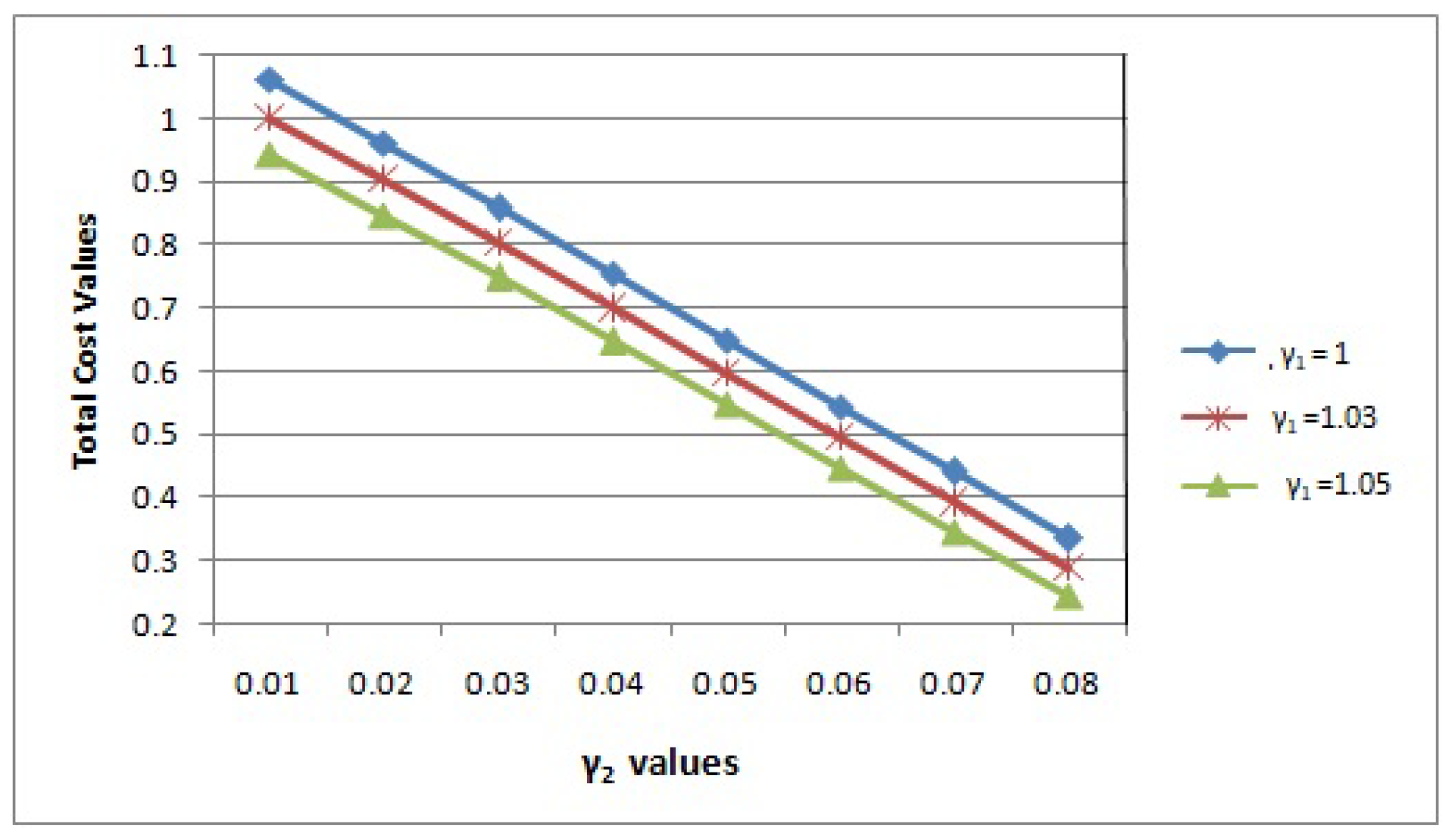
The impact of the second commodity perishable rate ( γ 2 ) on the TCR is shown in Figure 1 via three curves which relate to γ 1 = 1 , 1.03 , 1.05 . We discovered that the TCR diminishes whenever the perishable rate of the first commodity ( γ 1 ) and the perishable rate of the second commodity ( γ 2 ) increase.
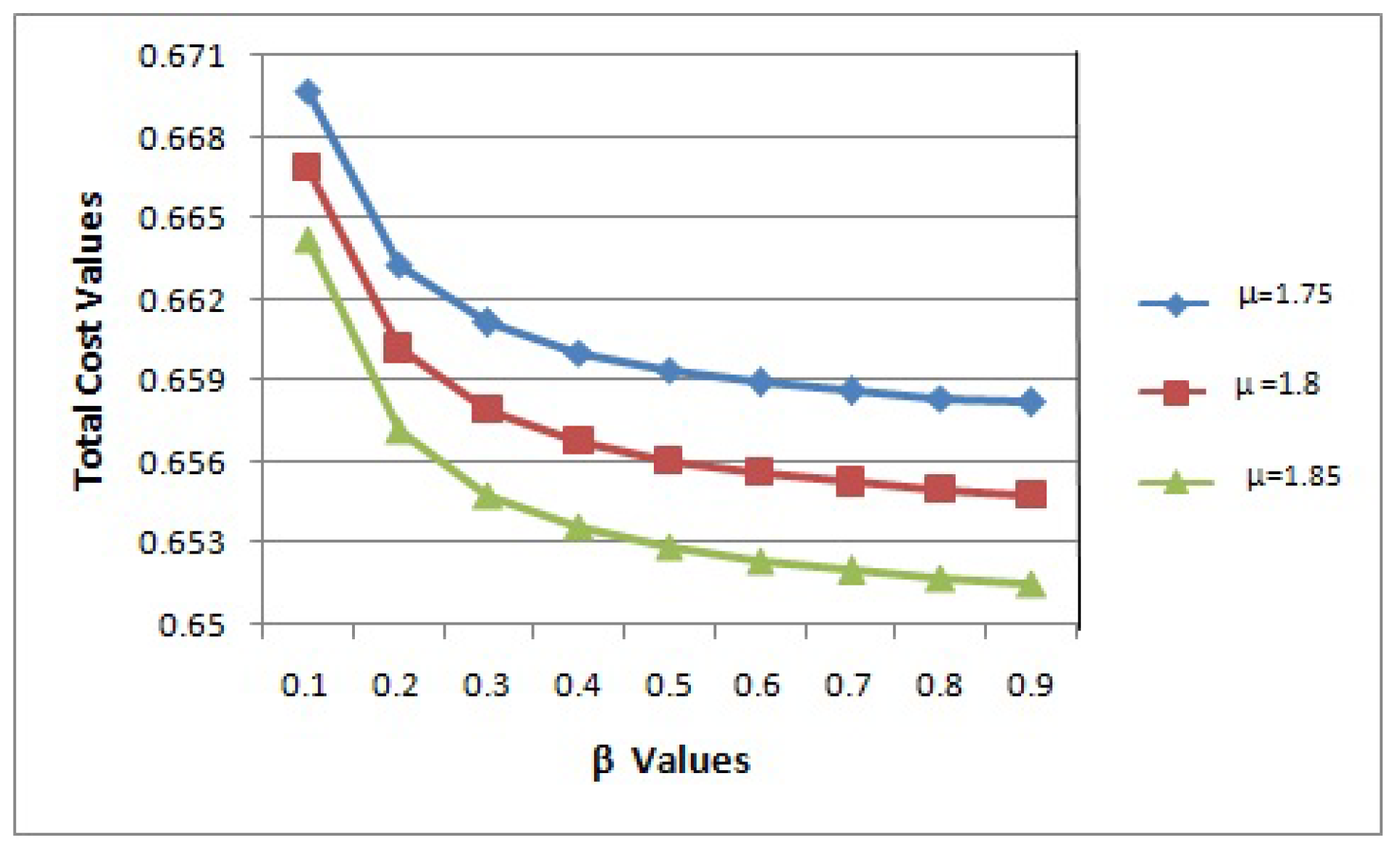
The outcome of the replenishment rate ( β ) on the TCR is depicted in Figure 2 via three curves which relate to ( μ ) = 1.75 , 1.8 , 1.85 . We discovered that the TCR diminishes whenever the service rate ( μ ) and the replenishment rate ( β ) increase.
In Table 7, Table 8 and Table 9, we demonstrate the outcome of the setup cost C S and the carrying cost of the first commodity C C 1 , and, similarly, the second commodity C C 2 on the optimal point ( S 1 * , s 1 * ) and the corresponding TCR T C . The other parameters and cost values are S 1 = 19 , S 2 = 18 , F = 4, s 1 = 5 , s 2 = 2 , γ 1 = 1.01 , γ 2 = 0.05 , α = 0.01 ; b 1 = 0.4 , b 2 = 0.32 , b 3 = 0.28 , C C 1 = 1.09 , C C 2 = 0.35 , C P 1 = 1.28 , C P 2 = 2.78 , C S = 1.77 ;
From the Table 7, Table 8 and Table 9, we discover the monotonic behavior of ( S 1 * , s 1 * ) as detailed below:
In Table 7, the TCR increases whenever both the carrying cost of the first commodity C C 1 and the second commodity C C 2 increases. In Table 8, the TCR increases when the carrying cost of the first commodity C C 1 and C S both increase. Similarly, Table 9 shows that the TCR increases whenever the carrying cost of the second commodity C C 2 and C S both increase. In addition, ( S 1 * , s 1 * ) monotonically decrease for all the Table 7, Table 8 and Table 9. The carrying cost, as well as the set-up cost, are components of the TC function, so, whenever the holding cost and setup cost increase, the total cost value also increases.
Furthermore, acquiring a significant amount of inventory increases a company’s carrying costs, whereas ordering smaller amounts of items more regularly increases a company’s setup costs. However, we want to minimize both costs so the TC is determined to do this work.

8. Conclusions

In this article, we studied a two-commodity inventory system that consists of a finite waiting hall. We investigated performance analyses of a perishable ( s , Q ) queueing-inventory system of two commodities with optional demands from customers. To obtain either a single item or only service without items, customer arrivals are analyzed using the MAP. We also obtained a steady-state vector. Furthermore, the outcomes were exemplified with numerical patterns to determine the convexity of the TCR. Similarly, we provided a numerical illustration that depicts the effect of the service rate on the inventory system’s TCR. In the numerical illustration, it is shown that the TCR diminishes because the service rates and replenishment rates are increased. The model describes the contribution of customers’ optional demands to the two-commodity system. We believe that the model portrayed and the investigation described have implications for a range of modern organisations since there are various kinds of customer demands, such as service requests without items. In the future, our proposed model can be used to explore more conditions, such as service and lead times under PH distribution, to assess whether customer arrivals might follow a batch Markovian arrival process, and to determine whether the server might also work under a vacation policy.

Author Contributions

Conceptualization, N.A.; data curation, R.S. and V.V.; formal analysis, N.A. and S.A.; funding acquisition, G.P.J. and B.S.; methodology, R.S.; project administration, B.S.; resources, B.S.; software, V.V.; supervision, G.P.J. and B.S.; validation, S.A.; writing—original draft, N.A.; writing—review and editing, G.P.J. All authors have read and agreed to the published version of the manuscript.

Funding

The present research has been conducted by the Research Grant of Kwangwoon University in 2022.

Institutional Review Board Statement

Not applicable.

Informed Consent Statement

Not applicable.

Data Availability Statement

The data presented in this study are available within the article.

Acknowledgments

Anbazhagan and Amutha would like to thank RUSA Phase 2.0 (F 24-51/2014-U), DST-FIST (SR/FIST/MS-I/2018/17) and DST-PURSE 2nd Phase programme (SR/PURSE Phase 2/38), Govt. of India.

Conflicts of Interest

The authors declare no conflict of interest.

Abbreviations

0Zero matrix with appropriate dimension.
eColumn vector of 1’s with appropriate dimension.
IIdentity matrix of appropriate order.
W i j Entry at (i,j)th position of a matrix W .

References

  1. Balintfy, J.L. On a basic class of multi-item inventory problems. Manag. Sci. 1964, 10, 287–297. [Google Scholar] [CrossRef]
  2. Silver, E.A. A control system for coordinated inventory replenishment. Int. J. Prod. Res. 1974, 12, 647–671. [Google Scholar] [CrossRef]
  3. Krishnamoorthy, A.; Iqbal Basha, R.; Lakshmy, B. Analysis of a two commodity inventory problem. Inf. Manag. Sci. 1994, 5, 127–136. [Google Scholar]
  4. Anbazhagan, N.; Arivarignan, G. Analysis of two commodity Markovian iventory system with lead time. Korean J. Comput. Appl. Math. 2001, 8, 427–438. [Google Scholar] [CrossRef]
  5. Anbazhagan, N.; Arivarignan, G.; Irle, A. A Two-commodity continuous review inventory system with substitutable items. Stoch. Anal. Appl. 2012, 30, 1–19. [Google Scholar] [CrossRef]
  6. Anbazhagan, N.; Goh, M.; Vigneshwaran, B. Substitutable inventory systems with coordinated reorder levels. J. Stat. Appl. Prob. 2015, 2, 221–234. [Google Scholar]
  7. Karthikeyan, K.; Sudhesh, R. Recent review article on queueing inventory systems. Res. J. Pharm. Technol. 2016, 9, 1451–1461. [Google Scholar] [CrossRef]
  8. Krishnamoorthy, A.; Lakshmy, B.; Manikandan, R. A survey on inventory models with positive service time. Opsearch 2011, 48, 153–169. [Google Scholar] [CrossRef]
  9. Sivakumar, B.; Anbazhagan, N.; Arivarignan, G. A two commodity perishable inventory system. Orion 2005, 21, 157–172. [Google Scholar] [CrossRef]
  10. Benny, B.; Chakravarthy, S.R.; Krishnamoorthy, A. Queueing-Inventory System with Two Commodities. J. Indian Soc. Probab. Stat. 2018, 19, 437–454. [Google Scholar] [CrossRef]
  11. Ozkar, S.; Uzunoglu Kocer, U. Two-commodity queueing-inventory system with two classes of customers. Opsearch 2020, 58, 234–256. [Google Scholar] [CrossRef]
  12. Senthil Kumar, P. A finite source two commodity inventory system with retrial demands and multiple server vacation. J. Phys. Conf. Ser. 2021, 1850, 012101. [Google Scholar] [CrossRef]
  13. Sinu Lal, T.S.; Joshua, V.C.; Vishnevsky, V.; Kozyrev, D.; Krishnamoorthy, A. A Multi-Type Queueing Inventory System: A Model for Selection and Allocation of Spectra. Mathematics 2022, 10, 714. [Google Scholar] [CrossRef]
  14. Senthil Kumar, P.; Mayil Vaganan, B. Two commodity inventory system with variable ordering quantity. AIP Conf. Proc. 2020, 2261, 030026. [Google Scholar]
  15. Yadavalli, V.S.S.; Adetunji, O.; Sivakumar, B.; Arivarignan, G. Two-commodity perishable inventory system with bulk demand for one commodity. S. Afr. J. Ind. Eng. 2010, 21, 137–155. [Google Scholar] [CrossRef]
  16. Nahmias, S. Perishable Inventory Systems; Springer: New York, NY, USA, 2011. [Google Scholar]
  17. Murthy, S.; Ramanarayanan, R. Two (s,S) Inventory Systems with Binary Choice of Demands and Optional Accessories with SCBZ Arrival Property. Int. J. Contemp. Math. Sci. 2009, 4, 397–417. [Google Scholar]
  18. Kocer, U.U.; Yalcin, B. Continuous review (s,Q) inventory system with random lifetime and two demand classes. Opsearch 2020, 57, 104–118. [Google Scholar] [CrossRef]
  19. Jacob, J.; Shajin, D.; Krishnamoorthy, A.; Vishnevsky, V.; Kozyrev, D. Queueing-Inventory with One Essential and m Optional Items with Environment Change Process Forming Correlated Renewal Process (MEP). Mathematics 2022, 10, 104. [Google Scholar] [CrossRef]
  20. Lucantoni, D.M.; Meier-Hellstern, K.S.; Neuts, M.F. A Single Server Queue with Server Vacations and a Class of Non-renewal Arrival Processes. Adv. Appl. Probab. 1990, 22, 676–705. [Google Scholar] [CrossRef]
  21. Latouche, G.; Ramaswami, V. Introdution to Matrix Analytic Methods in Stochastic Modelling; SIAM: Philadelphia, PA, USA, 1999. [Google Scholar]
  22. Lee, G.; Jeon, J. A New Approach to an N/G/1 Queue. Queueing Syst. 2000, 35, 317–322. [Google Scholar] [CrossRef]
  23. Chakravarthy, S.; Dudin, A. Analysis of a Retrial Queueing Model with MAP Arrivals and Two types of Customers. Math. Comput. Model. 2003, 37, 343–363. [Google Scholar] [CrossRef]
Figure 1. TC versus γ 2 . S 1 = 19 , S 2 = 18 , F = 4, s 1 = 5 , s 2 = 2 , β = 0.3 , μ = 1.7 , α = 0.01 ; b 1 = 0.4 , b 2 = 0.32 , b 3 = 0.28 , C C 1 = 1.09 , C C 2 = 0.35 , C P 1 = 1.28 , C P 2 = 2.78 , C S = 1.77 .
Mathematics 10 01801 g001
Figure 2. TC versus μ . S 1 = 19 , S 2 = 18 , F = 4, s 1 = 5 , s 2 = 2 , γ 1 = 1.01 , γ 2 = 0.05 , α = 0.01 ; b 1 = 0.4 , b 2 = 0.32 , b 3 = 0.28 , C C 1 = 1.09 , C C 2 = 0.35 , C P 1 = 1.28 , C P 2 = 2.78 , C S = 1.77 .
Mathematics 10 01801 g002
Table 1. Literature review overview.
Author(s)Poisson ArrivalsMAP ArrivalsJoint ReplenishmentOptional DemandExponentially Distributed
Lead Time
Perishable Inventory
Balintfy [1]
Silver [2]
Krishnamoorthy [3]
Anbazhagan [4]
Anbazhagan [5]
Anbazhagan [6]
Karthikeyan [7]
Krishnamoorthy [8]
Sivakumar [9]
Benny [10]
Ozkar [11]
Senthil Kumar [12]
Sinu Lal [13]
Senthil Kumar [14]
Yadavalli [15]
Nahmias [16]
Murthy [17]
Uzunoglu Kocer [18]
Jacob [19]
Lucantoni [20]
Latouche [21]
Lee [22]
Chakravarthy [23]
This paper
✓ Factors included in the research.
Table 2. TCR as a function of S 1 and S 2 .
S 1 / S 2 1314151617
200.958160.933120.914610.914290.99542
210.932390.787970.667730.566980.68216
220.929000.860210.850430.848900.90087
230.980220.946790.907400.901050.90133
241.103830.960210.941001.482301.49438
Table 3. TCR as a function of S 1 and F.
S 1 / F 56789
50.80650.76420.75121.14711.3590
60.76310.69910.71721.13191.3489
70.80250.69440.70811.12811.3487
80.82770.70620.70731.12251.3438
90.83760.71360.71141.12321.3430
100.84130.71650.71371.12461.3434
110.84260.71760.71461.12541.3439
Table 4. TCR as a function of S 2 and F.
S 2 / F 56789
120.762050.728860.725670.719250.84315
130.691720.635630.632800.589650.61770
140.734780.657980.649080.597180.61275
150.813030.692130.668180.607170.62222
160.815990.762430.736140.718500.73127
Table 5. TCR as a function of S 1 and s 1 .
S 1 / s 1 2345678
180.672080.669550.659550.654360.652220.651900.65216
190.656500.652870.650730.648930.648940.650070.65168
200.668380.652960.653850.657680.662570.667860.67321
210.702940.701540.663670.664870.670060.680210.69014
220.788440.775100.767280.765710.681730.682430.69431
Table 6. TCR as a function of S 2 and s 2 .
S 2 / s 2 23456
150.582600.579200.579420.581090.59306
160.582040.571380.572260.580040.58615
170.581230.580380.580450.595800.60113
180.592350.585500.588570.598550.60828
190.675020.596280.599790.601560.60891
Table 7. Impact of C C 1 and C C 2 costs on the optimal values.
C C 1 / C C 2 0.330.340.350.360.37
21 5 21 5 21 521 5 21 5
1.070.508960.549670.590390.631100.67181
21 5 21 5 21 5 19 5 19 5
1.080.545200.585920.626630.663100.69720
19 519 5 19 5 19 5 19 5
1.090.580740.614830.648930.683030.71713
15 5 15 5 15 5 15 5 15 5
1.100.600660.634760.702960.737060.76484
15 5 15 5 15 5 15 4 15 4
1.110.643490.712330.722890.784820.81679
Table 8. Impact of C C 1 and C S costs on the optimal values.
C C 1 / C S 1.751.761.771.781.79
20 5 20 5 20 5 20 5 20 5
1.070.592570.593420.594260.595100.59594
20 5 20 5 20 5 20 5 20 5
1.080.622920.623770.624610.632450.64230
20 5 20 5 19 5 19 5 19 5
1.090.633270.634120.648930.662410.67195
19 5 15 5 15 5 15 5 15 5
1.100.685200.689190.695010.695910.69821
18 5 15 5 15 5 15 415 4
1.110.686630.697700.698770.699500.70116
Table 9. Impact of C C 2 and C S costs on the optimal values.
C C 2 / C S 1.751.761.771.781.79
20 6 20 6 20 6 20 6 20 5
0.330.571820.575660.579500.589340.59919
20 5 20 5 20 5 20 5 20 5
0.340.615550.616290.617230.626070.62692
19 5 19 5 19 5 19 5 19 5
0.350.651870.655780.648930.667580.67748
19 5 15 5 15 5 15 5 15 5
0.360.690120.693360.703590.710810.73876
18 5 15 5 15 5 15 415 4
0.370.735020.751620.785090.795300.79741
Publisher’s Note: MDPI stays neutral with regard to jurisdictional claims in published maps and institutional affiliations.

