1. Introduction
Polymer coatings on implants and other biomedical devices are frequently used as local drug delivery systems, which allows for in situ release in the immediate targeted tissue, optimizing the therapeutic effects. Medications can be released at controlled rates in the range of effective treatment levels, increasing their bioavailability [
1]. In this sense, mathematical modeling of drug delivery and release predictability is useful in development and understanding of drug release mechanisms from controlled delivery systems. In most cases, drug diffusional mass transport is the predominant step in the control of drug release, while in others it is present in combination with polymer swelling or polymer erosion [
2]. In general, it is common to use power law equations for modeling release kinetics, such as the Higuchi and Ritger–Peppas models.
The Higuchi model [
3] implies various assumptions, namely, that the initial drug concentration in the polymer is higher than the drug’s solubility, that drug diffusion occurs in only one dimension (i.e., the edge effect must be negligible), that the drug particles are smaller than the polymer thickness, that matrix swelling and dissolution are negligible, that drug diffusivity is constant, and that perfect sink conditions are always attained. The Higuchi equation is provided by
where the ratio
is the fraction of drug released at time
t and
k is the Higuchi dissolution constant, which represents a Fickian diffusion of drugs without the matrix dissolution.
The Ritger–Peppas model [
4] is a simple relationship to describe drug release from a polymeric system. This model analyzes both Fickian and non-Fickian release of drug from swelling as well as non-swelling materials; however, it is only applicable up to 60% of the drug amount released. The Ritger–Peppas release equation is provided by
where the ratio
is the fraction of drug released at time
t,
k is the Ritger–Peppas kinetic constant, which characterizes the drug–matrix system, and
n is the exponent that indicates the drug release mechanism.
These semi-empirical models are easy to use and the established empirical rules help to explain transport mechanisms. However, they do not provide further insights into a more complex transport mechanism. Furthermore, these models might fail when specific experimental methodology or physicochemical processes are involved [
5]. For this reason, it is important to develop a mathematical model to adequately study the release kinetics from polymer coatings to liquid media. In this regard, this work is about a mathematical model that describes drug delivery considering a unidirectional iterative diffusion process in Fick’s second law while considering the convective phenomena from the polymer matrix to the liquid where the drug is delivered and the polymer–liquid drug distribution equilibrium. The resulting model is solved using Laplace transformation for two scenarios: (1) a constant initial condition for a single drug delivery experiment; and (2) a recursive delivery process where the liquid medium is replaced with fresh liquid after a fixed period of time, causing a stepped delivery rate. Finally, the proposed model is validated with experimental data.
2. Model Formulation
The main goal of the following model is to understand the drug release mechanisms from controlled delivery systems. Thus, the model must be able to evaluate whether the delivery system is controlled by the diffusion of the drug in the solid matrix (usually a polymer), by convection from the polymer surface to the liquid, or by the solid–liquid drug distribution equilibrium. In particular, we are interested in the experimental configuration shown in
Figure 1, where a polymer coating (solid matrix in the following) on an implant initially impregnated with the drug is immersed in a volume of liquid,
, for a fixed period of time, producing a time-varied drug concentration in the liquid bulk,
, that can be measured.
In order to model drug delivery, the following assumptions are considered:
Drug diffusion is only in one dimension, x (i.e., the edge effect must be negligible); therefore, the concentration of the drug in the solid matrix is expressed as
Drug particles (solute) are smaller than solid thickness
Matrix swelling and dissolution are negligible, therefore, the length of the diffusion region, , is constant, and by symmetry the problem is analyzed in the following domain:
Drug diffusivity in the solid matrix, D, is constant and Fick’s law can be applied, i.e.,
There exists an equilibrium between the concentration of the drug in the interface of the solid matrix and the liquid, provided by
There is a convective rate that depends on the difference of the concentration in the solid–liquid interface, , and the equilibrium concentration, , with the form
The entire surface of the solid is completely submerged.
In the following sections, a model is developed for two scenarios: (1) a constant initial condition for a single drug delivery experiment; and (2) a recursive delivery process where the liquid medium is replaced with fresh liquid after a fixed period of time, causing a stepped delivery rate.
2.1. Single Drug Delivery Experiments
Consider a unidirectional diffusion of the solute in the solid matrix, described by the following partial differential equation:
where
D is the diffusivity and
L is the length. The initial condition is
and boundary conditions are
where
is the solute concentration in the liquid,
is the mass transfer coefficient in the liquid, and
is the solute solid–liquid partition coefficient associated with the equilibrium. Condition (
2) indicates that the initial concentration in the solid matrix is homogeneous and equal to
. Condition (
3) appears due to the symmetry of diffusion in the middle of the solid, while condition (
4) represents the solid–liquid interface. The accumulation of the solute in the liquid can be easily obtained from the mass balance,
where
A is the area of mass transport and
is the volume of the liquid. The total solute mass in the solid matrix and the liquid is constant and equal to
where
is the initial solute mass in the solid matrix and, assuming that initially the solute concentration in the liquid is zero
, it is equivalent to
Notice that the time derivative of Equation (
6) provides
and considering Equation (
1) and boundary condition (
3), the previous equation becomes
which agrees with the substitution of Equation (
4) in Equation (
5). The mass of the solute in the liquid is therefore
where
is the total mass of the solute in the solid matrix. Finally, replacing Equation (
8) in boundary condition (
4), it follows that
where
and
are the Sherwood number, which represents the ratio of convective mass transfer to the rate of diffusive mass transport.
2.2. Recursive Delivery Experiment
Now, let us consider an iterative process where for each fixed period of time
the liquid is replaced by fresh liquid without solute. Then, the iterative process can be modeled by the diffusion equation,
with an initial condition that depends on the concentration of the previous iteration:
and the following boundary conditions:
where
and the initial mass of the solute in the solid at iteration
k depends on the final concentration of iteration
, i.e.,
To analyze the iterative behavior, it is proposed that a shift in time
be defined in such a way that the previous model becomes
for
. Then, the analytical solution of the models for the two scenarios is presented in the following section using Laplace transformation [
6].
5. Discussion
The proposed models for single and recursive release experiments presented in
Section 2.1 and
Section 2.2, respectively, are general and allow us to clarify the predominant step in the control of drug release, This is because these models consider the drug diffusion in the solid matrix, the convective phenomenon from the solid matrix to the liquid, where the drug is delivered, and the solid–liquid drug distribution equilibrium. In particular, considering the experimental conditions of the study case presented in
Section 4, diffusion dominates over convection thanks to the mixing conditions established by the horizontal shaker (with 100 rpm) in our experiments. For this reason, we was obtained
, reducing the number of parameters to two, namely,
; however, convection might be relevant as well for in situ applications.
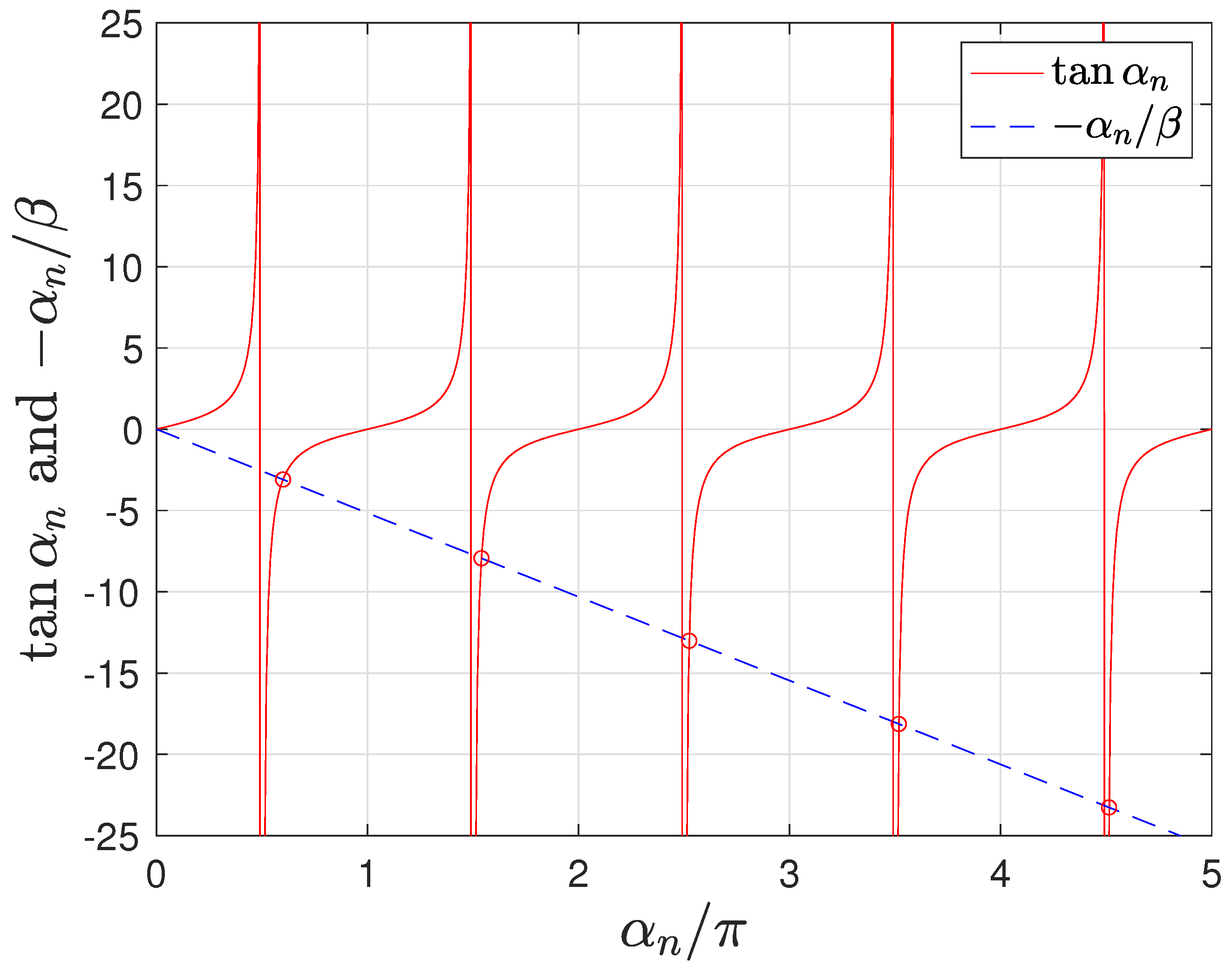
In the Higuchi model [
3], the characteristic values are of the form
, leading to the approximation
. However, the assumption of solid–liquid interface equilibrium leads to the characteristic Equation (
23), which depends on both Sh and
and the characteristic values of which must be numerically computed. In particular, for
and
the first characteristic values are
,
,
,
,…, which tends towards
as
n increases (see
Figure 4). The deviation from
of the first characteristic values produces a response that is non necessarily proportional to
, as in the Higuchi model [
3].
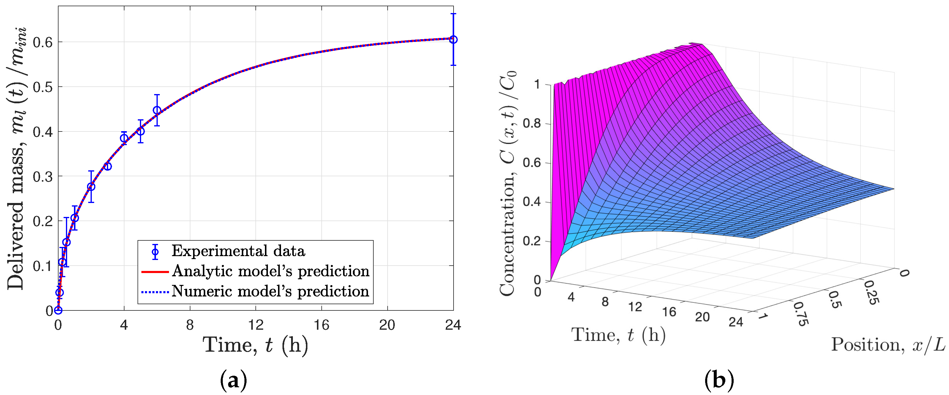
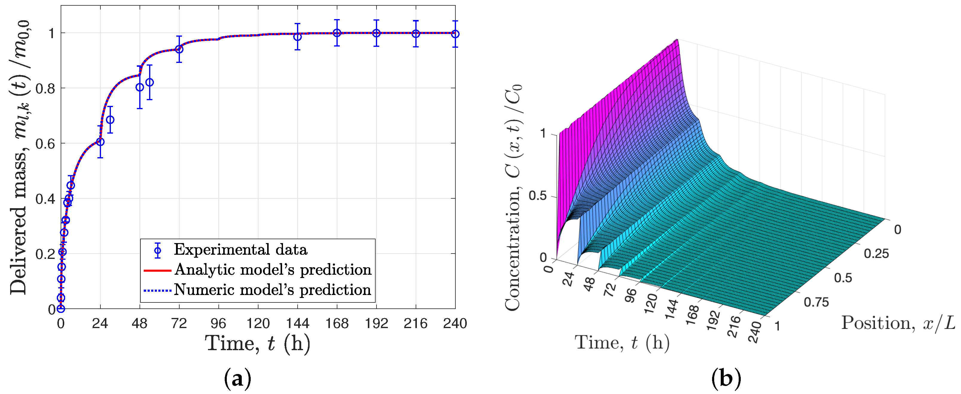
The experimental evidence shown in
Figure 2a and
Figure 3a supports the use of the solid–liquid interface equilibrium assumption,
, because at the end of the first 24 h the concentration in the liquid seems to reach a constant value (see
Figure 2a); it was only after the PBS medium was exchanged for a fresh one that the drug release continued (see
Figure 2a). Condition (
9) or its equivalent for the recursive delivery (
17) includes the solid–liquid interface equilibrium assumption, and these conditions indicate that the rate of drug delivery to the liquid is time-varyiant, as it depends on the total mass of the drug in the liquid at the same instant. This concentration is proportional to the total mass inside the solid matrix due to the total mass balance of the total solid–liquid system. As a result of these conditions, the delivered mass with respect to the initial mass within the solid matrix tends to
as time tends to infinity (see Equation (
32)), which is consistent with the experimental data, i.e.,
for
. Thus, for the particular experimental study case, when the drug concentration in the liquid is low, diffusion controls the delivery rate; however, as this concentration increases, the equilibrium plays a greater role, becoming the controlling mechanism as time increases.
The proposed models for single or recursive delivery are able to describe the delivered mass profile (see
Figure 2a and
Figure 3a), that is, the usual experimental measurement, and allows prediction of the concentration profile within the solid matrix, as shown in
Figure 2b and
Figure 3b. Notice that for the particular experimental study case, after each 24 h the profile concentration in the solid matrix is approximately constant, because the solid–liquid interface equilibrium has been reached. In addition, in order to validate the analytical solutions provided in Equation (
32) for single release experiments and Equation (
40) for recursive release experiments, numerical solutions of the proposed models were determined using an orthogonal collocation method;
Figure 2a and
Figure 3a show that the numerical and analytical solutions overlap.
6. Conclusions
In this work, a mathematical model to describe drug delivery from polymer coatings on implants was proposed. The model considers a unidirectional recursive diffusion process which follows Fick’s second law and considers the convective phenomena from the polymer matrix to the liquid where the drug is delivered as well as the polymer–liquid drug distribution equilibrium. The resulting model is solved using Laplace transformation for two scenarios: (1) a constant initial condition for a single drug delivery experiment; and (2) a recursive delivery process where the liquid medium is replaced with fresh liquid after a fixed period of time, causing a stepped delivery rate. Finally, the study case shows that these models can satisfactorily reproduce the experimental data, clarifying the predominant step in the control of drug release.
The proposed models for single and recursive release experiments presented in
Section 2.1 and
Section 2.2 have linear partial differential equations and boundary conditions; therefore, it was possible to obtain the analytical solutions provided in Equations (
25), (
31) and (
32) for single release experiments, and Equations (
39) and (
40) for recursive release experiments. However, numerical methods are another option to solve these problems, and they become mandatory when extra phenomena need to be included in the drug release models in order to obtain satisfactory predictions, for instance, when swelling and degradation of the solid matrix become relevant, causing moving boundaries, or when a drug has more complex interactions such as biodegradation or adsorption, which produce non-linear terms in the model due to the reaction kinetics or adsorption isotherms.


 and
and 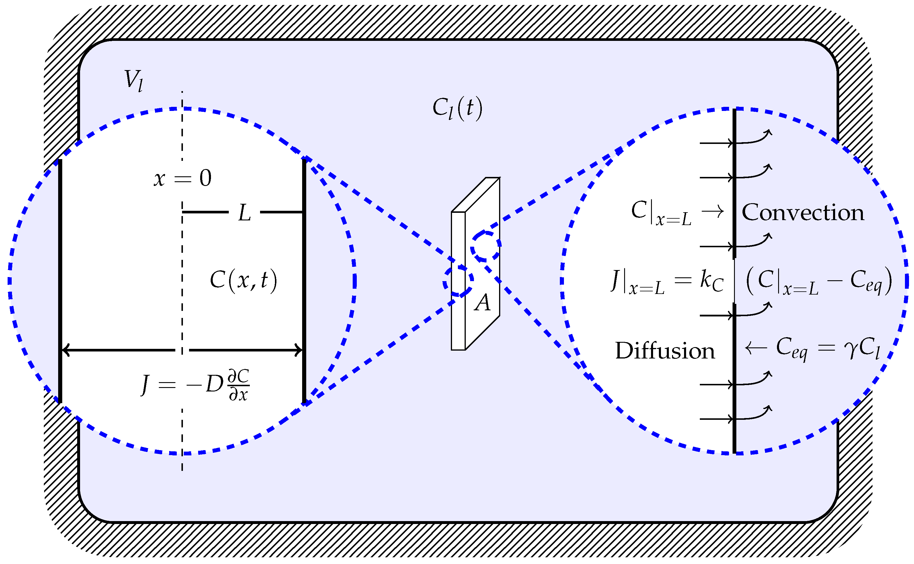


