Traveling Band Solutions in a System Modeling Hunting Cooperation

Abstract

A classical Lotka–Volterra model with the logistical growth of prey-and-hunting cooperation in the functional response of predators to prey was extended by introducing advection terms, which included the velocities of animals. The effect of velocity on the kinetics of the problem was analyzed. In order to examine the band behavior of species over time, traveling wave solutions were introduced, and conditions for the coexistence of both populations and/or extinction were found. Numerical simulations illustrating the obtained results were performed.

1. Introduction

Population dynamics is an active research field in mathematical biology, aimed at studying and predicting the evolution of ecosystems as a consequence of different dynamic behaviors. When considering ecological communities, along with interspecific interactions, such as predation and competition, intraspecific interactions (both aggressive and cooperative) can provide new insights for modeling more complex dynamics. Cooperation, indeed, can be observed in many biological systems and is known to induce demographic Allee effects [1]. In particular, cooperative hunting, observed in many species (carnivores, birds, aquatic organisms, spiders), often increases hunting success: this phenomenon, the Allee effect in predators, can sensibly alter the stability of the ecological community, by either allowing the survival of predators that would go extinct otherwise or increasing predation pressure and leading to a drastic prey decrease [2]. The population growth is strongly influenced by both environmental factors [3] and species density. The spatial structure of the environment affects individual movements, with consequences on population dynamics. Individual movements can be undirected or directed. The random movement of individuals in the environment is generally modeled as a passive diffusion of a density function. To describe such a random movement of individuals in both prey and predator populations, self-diffusion terms can be introduced in the model. Along with these modifications, cross-diffusion terms can be considered to take into account how the random movement of one population can be influenced by the presence or absence, abundance or scarcity of individuals belonging to the other species [4,5,6]. These reaction–-diffusion models have been widely used to describe the spatiotemporal behavior of similar systems in different fields, from chemical to economic as well as biological [7,8,9,10,11,12].

Previous work by our research team has considered some interacting population models and investigated several characteristics (e.g., scarcity of resources, nonlinear growth, fear effect, cooperative predation), also in the context of a spatially inhomogeneous environment. In previous research, the authors considered and analyzed ODE representations for the spreading of waterborne diseases (for example [13]) and reaction–-diffusion systems modeling a predator–prey community with either hunting cooperation [14,15] or fear and group defense [16]. These last models helped to highlight the effect of spatial diffusion on the evolution of an ecosystem, and its role in the appearance of spatial patterns in equilibrium states. Conditions on the model parameters leading to the presence of such patterns and to the specification of their aspect (stripes, spots, etc.) have also been obtained.

In some contexts, individuals belonging to a population can have advective (directed) movements either driven by a directional fluid/wind flow or arising from their senses and following the gradient of a resource distribution (taxis); in other contexts, species move towards (or away from) other species to compete for food, or to escape and survive. Some examples of this directed movement can be found in living species in rivers, lakes, and oceans, as well as in marine species along coastlines. Various advection models have been formulated in order to highlight the possible different types of taxis, with or without the additional presence of random dispersion (e.g., [17,18,19,20,21,22,23,24] and the references therein). It has been observed (e.g., [25]) that often animals move aggregated in groups or bands. Many studies have been conducted to highlight collective trends and interactions between different individuals and different species (e.g., [26,27] and the references therein). Several authors have developed models and techniques aimed at capturing the above collective behavior of these species. Among these techniques, traveling waves can be found in various studies to describe the aggregation of microorganisms in chemotaxis phenomena [28], in studies of cell movement phenomena in the evolution of wound healing [29], and in studies of movement and cohesion in insect swarms [30]. On the contrary, they have been used little in studies concerning the behavior of other categories of animals in prey–predator dynamics. Generally, traveling wave solutions have been interpreted as a spatial distribution (i.e., as dispersion rather than clustering); consequentially, they have not been used often to study the temporal dynamics in ecological systems. In such spatial models, the coexistence problem can also depend on the characteristics of the domain in which the populations live. From another point of view, traveling waves could represent good candidates to describe the temporal dynamics in the movement of animal bands [4,5] In this paper, we used traveling wave solutions to analyze the band behavior of prey and predator species over time. We firmly believed that studying the behavior of each band and the interactions between them could be useful to provide a clear overview of the evolution of the system. In order to represent individual and collective movements and analyze how the velocity of individuals affected their competition and the coexistence of competitors and influenced the kinetics of the system in general, a taxis model was considered. In this model, the predator–prey system with hunting cooperation, as introduced in [2], was extended to include an advection term where each individual of both species moved with its own velocity. We emphasize that the advection terms were introduced in the ODE system in order to evaluate the influence of individual velocity alone on the kinetics of the system. Adding advection to the system could change the long-term outcome (coexistence/extinction) of the population. As an example, as compared to the ODE system, in a scenario in which the predation pressure was strong while, at the same time, the prey population moved slowly, it was possible to reach the extinction of both species. Once we have assessed the contribution due to advection terms, we also plan to consider a diffusive advection system in a future study, in order to evaluate the combined effect of both directed movement and random dispersion.

Note that in [14,15], the authors extended the model in [2] to include spatiotemporal dynamics; they studied the effect of diffusion and explored the related Turing patterns formation. Later, in [31], the influence of cross-diffusion was analyzed. In [32], the authors replaced the ordinary time derivative with a fractional one in order to investigate how the fractional-in-time derivative impacted the system dynamics, while in [33], traveling wave solutions of diffusive extension of the predator–prey model (with spatial diffusion of predators) were investigated.

Briefly, the novelty of this contribution was to introduce the effect of the collective movement of both populations in a predator–prey model whose complex kinetics already assumed hunting cooperation in the functional response of predators. Traveling waves, usually considered as a tool to describe the spatial distribution of species, were introduced to study the evolution of bands of each species over time, taking into account the interplay between the velocities of bands and individuals. Such a study provided challenges and ideas in many other fields of applied mathematics such as ecology, aerospace science, and economics, in which nonlinear mathematical models having a similar structure have been considered.

The paper is arranged as follows. Section 2 is devoted to preliminary results concerning the starting mathematical model and the statement of the problem. In Section 3, the traveling waves are introduced, and the stability analysis is performed, obtaining the main theorem that summarizes the influence of the velocity on the kinetics of the system. In Section 4, various numerical simulations are performed, painting rich scenarios. The paper ends with conclusions on the obtained results.

2. Mathematical Model

2.1. Preliminaries

In this section, we start with the model studied in [2], where the classical Lotka–Volterra with logistical growth of the prey had been extended by considering hunting cooperation in the functional response of predators to prey. Specifically, it was assumed that cooperative predators would benefit from their behavior, so that the success of their attacks increased with their density: the constant attack rate $\lambda$ of the classical model was replaced by a density-dependent term. The model is given by

$$\left\{\begin{array}{c}{\displaystyle \frac{du}{d\tau }=ru\left({\displaystyle 1-\frac{u}{k}}\right)-(\lambda +aw)uw,}\hfill \\ \\ {\displaystyle \frac{dw}{d\tau }=e(\lambda +aw)uw-mw,}\hfill \end{array}\right.$$

(1)

where $u\left(\tau \right)$ and $w\left(\tau \right)$ represent prey and predators densities, respectively; $r>0$ is the per capita growth of prey, $k>0$ is the carrying capacity of prey; $e>0$ is the food conversion efficiency; $m>0$ is the per capita mortality rate of predators; $\lambda >0$ is the attack rate; and $a>0$ is the predators’ rate of hunting cooperation. Then by adopting dimensionless variables and parameters, the non-dimensionalized version of the model is given by

$$\left\{\begin{array}{c}{\displaystyle \frac{dn}{dt}=\sigma n\left({\displaystyle 1-\frac{n}{K}}\right)-(1+\alpha p)np,}\hfill \\ \\ {\displaystyle \frac{dp}{dt}=(1+\alpha p)np-p,}\hfill \end{array}\right.$$

(2)

where $n\left(t\right)$ and $p\left(t\right)$ are prey and predator densities, respectively, and the three dimensionless parameters are obtained as

$${\displaystyle \sigma =\frac{r}{m};K=\frac{e\lambda k}{m};\alpha =\frac{am}{{\lambda }^2}.}$$

As observed in [2], K comprises the dimensional carrying capacity, the conversion efficiency, as well as the per-capita predator mortality and attack rate; then it could be interpreted as the predators’ basic reproduction number.

System (2) admits the steady states $E_0\equiv (0,0)$, $E_1\equiv (K,0)$ and the coexistent equilibria $E^{*}=(n^{*},p^{*})$, where

$${\displaystyle n^{*}=\frac{1}{1+\alpha p^{*}}}$$

(3)

and $p^{*}$ (positive) solution of

$$f\left(x\right):=K{\alpha }^2{x}^3+2\alpha K{x}^2+K(1-\sigma \alpha )x+\sigma (1-K)=0.$$

(4)

If $K>1$, then $E^{*}$ is unique; while if

$${\displaystyle \frac{-2-9\alpha \sigma +(2+6\alpha \sigma )\sqrt{1+3\sigma \alpha }}{\alpha \sigma (1+4\alpha \sigma )}<K\le 1,\sigma >\frac{1}{\alpha },}$$

(5)

then there exist two coexistent equilibria. In all other cases, no coexistent equilibria were admissible. Concerning the stability of the above steady states, the following theorem holds true.

Theorem 1.

The coexistent equilibrium $E^{*}\equiv (n^{*},p^{*})$ is stable when

$${\displaystyle \alpha K{p}^{*}<\sigma <\frac{K{(1+\alpha p^{*})}^2(1+2\alpha p^{*})}{\alpha }.}$$

(6)

The boundary equilibrium $E_0\equiv (0,0)$ is always unstable; the boundary equilibrium $E_1\equiv (K,0)$ is unstable if $K>1$ and stable if $K<1.$

This result easily follows from linear stability analysis. Indeed, the entries $a_{ij}$ of the Jacobian matrix J characterizing the linearized system close to the generic equilibrium $\overline{E}=(\overline{n},\overline{p})$ can be written as:

$$\left\{\begin{array}{cc}{a}_{11}=\sigma (1-\frac{2}{K}\overline{n})-(1+\alpha \overline{p})\overline{p},\hfill & a_{12}=-(1+2\alpha \overline{p})\overline{n},\hfill \\ a_{21}=(1+\alpha \overline{p})\overline{p},\hfill & a_{22}=(1+2\alpha \overline{p})\overline{n}-1.\hfill \end{array}\right.$$

(7)

The Jacobian matrix for $E_0$, $E_1$, and $E^{*}$ is given by:

$$J\left(E_0\right)=\left(\begin{array}{cc}\sigma & 0\\ 0& -1\end{array}\right);J\left(E_1\right)=\left(\begin{array}{cc}-\sigma & -K\\ 0& K-1\end{array}\right);$$

$$J\left(E^{*}\right)=\left(\begin{array}{cc}{\displaystyle \frac{-\sigma }{K(1+\alpha p^{*})}}& {\displaystyle -\frac{1+2\alpha p^{*}}{1+\alpha p^{*}}}\\ (1+\alpha p^{*})p^{*}& {\displaystyle \frac{\alpha p^{*}}{1+\alpha p^{*}}}\end{array}\right).$$

It is evident that the eigenvalues of $J\left(E_0\right)$ are $\{\sigma ,-1\}$, so that $E_0$ is a saddle point. $E_1$ is stable only for $K>1$, as $J\left(E_1\right)$ has $\{-\sigma ,K-1\}$ as eigenvalues. Finally, the requirements $\mathtt{tr}\left[J\left(E^{*}\right)\right]<0$ and $\mathtt{Det}\left[J\left(E^{*}\right)\right]>0$ lead to the two inequalities in (6). For ease of notation in the following analysis, we denote by

$${\displaystyle {\sigma }^{*}=\frac{K{(1+\alpha p^{*})}^2(1+2\alpha p^{*})}{\alpha }.}$$

(8)

2.2. The Advection Model

In order to describe and examine the effect of the individual-directed movement on the kinetics of the system, we generalized (2) by introducing advection terms. In particular, we introduced a velocity for each individual of both populations in order to represent the movement of individuals belonging to prey and predator populations

$$\left\{\begin{array}{c}{\displaystyle \frac{\partial n}{\partial t}+v_1·\nabla n=\sigma n\left({\displaystyle 1-\frac{n}{K}}\right)-(1+\alpha p)np,}\hfill \\ \\ {\displaystyle \frac{\partial p}{\partial t}+v_2·\nabla p=(1+\alpha p)np-p,t}\hfill \end{array}\right.$$

(9)

where $n(\mathbf{x},t)$ and $p(\mathbf{x},t)$ represent the densities of prey and predator population, $\mathbf{x}\in \Omega \subset {\mathbb{R}}^2$ and $t>0$. The parameters $v_1=(v_1^1,v_1^2)$ and $v_2=(v_2^1,v_2^2)$ are the average velocities of each (individual) prey and predator. We appended the initial boundary conditions

$$\left\{\begin{array}{cc}n(\mathbf{x},0)=n_0\left(\mathbf{x}\right),\hfill & p(\mathbf{x},0)=p_0\left(\mathbf{x}\right)\mathrm{on}\Omega \hfill \\ n(\mathbf{x},t)=\overline{n},\hfill & p(\mathbf{x},t)=\overline{p},\mathrm{on}\partial \Omega \times {\mathbb{R}}_{+}\hfill \end{array}\right.$$

(10)

where $\overline{n}$ and $\overline{p}$ are positive constants.

Remark 1.

The system (9) admits the same constant steady states of system (2) and of the diffusive system introduced in [14].

3. Traveling Waves: Stability Analysis

We introduce the following variables for the traveling waves analysis

$$z=-\kappa ·\mathbf{x}+ct,n(\mathbf{x},t)=\mathcal{N}\left(z\right),p(\mathbf{x},t)=\mathcal{P}\left(z\right),$$

(11)

where $\kappa =({\kappa }_1,{\kappa }_2)$ is the wave vector and c is the wave speed. System (9) becomes

$$\left\{\begin{array}{c}(c-\kappa ·v_1){\mathcal{N}}^{\prime }=\sigma \mathcal{N}\left({\displaystyle 1-\frac{\mathcal{N}}{K}}\right)-(1+\alpha \mathcal{P})\mathcal{N}\mathcal{P},\hfill \\ \\ (c-\kappa ·v_2){\mathcal{P}}^{\prime }=(1+\alpha \mathcal{P})\mathcal{N}\mathcal{P}-\mathcal{P}.\hfill \end{array}\right.$$

(12)

In view of (11), if the asymptotic behavior of (9) and (12) is the same ($z\to \infty ,t\to \infty$), then the asymptotic behavior analysis of the traveling waves $\mathcal{N}$ and $\mathcal{P}$ of (12) gives the description of the asymptotic behavior of (9). It is also worth highlighting that the existence of traveling waves of the most varied biological models (and not only) has been a well-studied topic in the literature (including diffusive terms, advection terms, time delays).

Denoting the generic steady state again by $\overline{E}\equiv (\overline{n},\overline{p})$ and by introducing the perturbation fields $\{U=\mathcal{N}-\overline{n},V=\mathcal{P}-\overline{p}\}$, the linear version of (12) is

$${\displaystyle \frac{\partial }{\partial t}\left(\begin{array}{c}U\hfill \\ V\hfill \end{array}\right)=\left(\begin{array}{cc}{\displaystyle \frac{a_{11}}{c-\kappa ·v_1}}& {\displaystyle \frac{a_{12}}{c-\kappa ·v_1}}\\ {\displaystyle \frac{a_{21}}{c-\kappa ·v_2}}& {\displaystyle \frac{a_{22}}{c-\kappa ·v_2}}\end{array}\right)\left(\begin{array}{c}U\hfill \\ V\hfill \end{array}\right)=A\left(\overline{E}\right)\left(\begin{array}{c}U\hfill \\ V\hfill \end{array}\right),}$$

(13)

where the expressions of $a_{ij}$ in the entries of this new Jacobian matrix A are the ones given in (7). The necessary and sufficient condition guaranteeing the linear stability [34] of $\overline{E}$ is

$$\mathtt{tr}\left[A\left(\overline{E}\right)\right]<0,\mathtt{Det}\left[A\left(\overline{E}\right)\right]>0.$$

(14)

The three equilibria were considered separately.

•

The Jacobian matrix A written near $E_0$ is

$$A\left(E_0\right)=\left(\begin{array}{cc}\frac{\sigma }{c-\kappa ·v_1}& 0\\ 0& \frac{-1}{c-\kappa ·v_2}\end{array}\right).$$

(15)

If for $c<\kappa ·v_2$ or $c>\kappa ·v_1$, at least one eigenvalue is positive, then the steady state $E_0$ is unstable. When $\kappa ·v_2<c<\kappa ·v_1,$ the condition (14) is satisfied, then $E_0$ is stable.

•

In the vicinity of $E_1$, the Jacobian matrix is

$$A\left(E_1\right)=\left(\begin{array}{cc}\frac{-\sigma }{c-\kappa ·v_1}& \frac{-K}{c-\kappa ·v_1}\\ 0& \frac{K-1}{c-\kappa ·v_2}\end{array}\right).$$

(16)

When $c<min(\kappa ·v_1,\kappa ·v_2)$, we can distinguish two cases: $K<1\mathtt{and}K>1$. When $K>1$, it follows that $\mathtt{Det}\left[A\left(E_1\right)\right]<0$; while if $K<1$, then it follows that $\mathtt{tr}\left[A\left(E_1\right)\right]>0;$ in both cases, $E_1$ is unstable.

When $\kappa ·v_2<c<\kappa ·v_1,$ the steady state $E_1$ is unstable. In fact, if $K>1$, then it follows that $\mathtt{tr}\left[A\left(E_1\right)\right]>0$; while if $K<1$, then it follows that $\mathtt{Det}\left[A\left(E_1\right)\right]<0.$

When $\kappa ·v_1<c<\kappa ·v_2,$ the steady state $E_1$ is unstable if $K<1$ being $\mathtt{Det}\left[A\left(E_1\right)\right]<0,$ while $E_1$ is stable if $K>1.$

•

In the vicinity of $E^{*}$, the Jacobian matrix can be written as

$$A\left(E^{*}\right)=\left(\begin{array}{cc}\frac{b_{11}}{c-\kappa ·v_1}& \frac{b_{12}}{c-\kappa ·v_1}\\ \frac{b_{21}}{c-\kappa ·v_2}& \frac{b_{22}}{c-\kappa ·v_2}\end{array}\right),$$

(17)

with

$$\left\{\begin{array}{cc}{\displaystyle b_{11}=-\frac{\sigma }{K(1+\alpha p^{*})},}\hfill & {\displaystyle b_{12}=-\frac{1+2\alpha p^{*}}{1+\alpha p^{*}},}\hfill \\ b_{21}=(1+\alpha p^{*})p^{*},\hfill & {\displaystyle b_{22}=\frac{\alpha p^{*}}{1+\alpha p^{*}}.}\hfill \end{array}\right.$$

(18)

In this case, we can write

$$\begin{array}{c}{\displaystyle \mathtt{tr}\left[A\left(E^{*}\right)\right]=\frac{1}{K(1+\alpha p^{*})}\left[{\displaystyle -\frac{\sigma }{c-\kappa ·v_1}+\frac{\alpha K{p}^{*}}{c-\kappa ·v_2}}\right],}\hfill \\ {\displaystyle \mathtt{Det}\left[A\left(E^{*}\right)\right]=\frac{1}{(c-\kappa ·v_1)(c-\kappa ·v_2)}\frac{p^{*}}{{(1+\alpha p^{*})}^{2}K}[-\alpha \sigma +K{(1+\alpha p^{*})}^2(1+2\alpha p^{*})].}\hfill \end{array}$$

(19)

When $\kappa ·v_1<c<\kappa ·v_2,$ being $\mathtt{t}\mathtt{r}\left[A\left(E^{*}\right)\right]<0$, then $E^{*}$ is stable (unstable) if and only if $\sigma >{\sigma }^{*}$ ($\sigma <{\sigma }^{*}$).

When $\kappa ·v_2<c<\kappa ·v_1,$ being $\mathtt{tr}\left[A\left(E^{*}\right)\right]>0$, then $E^{*}$ is unstable.

If $c<min(\kappa ·v_1,\kappa ·v_2),$ denoted by

$${\displaystyle \overline{\sigma }=\alpha K{p}^{*}\frac{c-\kappa ·v_1}{c-\kappa ·v_2},}$$

(20)

it follows that

$$\begin{array}{c}\mathtt{Det}\left[A\left(E^{*}\right)\right]>0(<0)\iff \sigma <{\sigma }^{*}(\sigma >{\sigma }^{*}),\hfill \\ \mathtt{tr}\left[A\left(E^{*}\right)\right]<0(>0)\iff \sigma <\overline{\sigma }(\sigma >\overline{\sigma }).\hfill \end{array}$$

(21)

Remark 2.

When $c>max(\kappa ·v_1,\kappa ·v_2)$, the asymptotic stability analysis for system (12) in the vicinity of the steady states is the same as we have reported for system (2).

The above results were summarized in the following theorem.

Theorem 2.

• When $c>\kappa ·v_1$ and $c<\kappa ·v_2$, the coexistent equilibrium $E^{*}$ is stable if $\sigma >{\sigma }^{*}$, and unstable otherwise.
• When $c>\kappa ·v_2$ and $c<\kappa ·v_1$, the coexistent equilibrium $E^{*}$ is unstable.
• If $c<min(\kappa ·v_1,\kappa ·v_2)$, then
  $E^{*}$ is stable $\iff \sigma <min\{{\sigma }^{*},\overline{\sigma }\}$ and unstable $\iff \sigma >max\{{\sigma }^{*},\overline{\sigma }\}.$
• If $c<\kappa ·v_2$ or $c>\kappa ·v_1$, then $E_0$ is unstable.
• If $c>\kappa ·v_2$ and $c<\kappa ·v_1$, then $E_0$ is stable.
• If $c<min(\kappa ·v_1,\kappa ·v_2)$ or $c>\kappa ·v_2$ and $c<\kappa ·v_1$, then $E_1$ is unstable.
• If $c>\kappa ·v_1$ and $c<\kappa ·v_2$, then $E_1$ is stable for $K>1$ and unstable for $K<1.$

From a biological point of view, recalling that $v_1$ and $v_2$ represent the average velocity of each member of prey and predator species, respectively, while c is the velocity at which a band of each species moves, we could provide a possible interpretation of the above results.

Unlike the ODE system for which the equilibrium $E_0$ would always be unstable, when the velocities of the individuals of both species were considered, the equilibrium $E_0$ could be stable. In particular, when the velocity of a band of predators was greater than the average speed of any member of the predator population ($c>\kappa ·v_2$), that is, the band would move rapidly to catch a prey, increasing the predation pressure; and at the same time, if the velocity at which a band of prey moved was smaller than the average velocity of any individual of that species ($c<\kappa ·v_1$), that is, the prey population moved slowly, not perceiving predatory pressures, then it would be possible to reach the extinction of both species. In this case, consistently, the coexistent equilibrium was always unstable.

Concerning the coexistent equilibrium, we noted that when the velocity of the band of predators was smaller than the average speed of any member ($c<\kappa ·v_2$), that is, the band moved slowly to catch a prey, reducing the predation pressure, and at the same time, the velocity at which a band of prey moved was greater than the average velocity of any individual of the prey species ($c>\kappa ·v_1$), that is, the prey population was more interested in security, the same condition ensuring the stability of $E^{*}$, according to Theorem 1, implied the instability of $E^{*}$, according to Theorem 2.

4. Numerical Simulations

In order to graphically represent our findings on the stationary states of the considered model (9), we first thoroughly explored the parameter space to identify suitable regions corresponding to the stability/instability of the equilibria in the related cases. Clearly, different values of the predators’ basic reproduction number K (higher or lower than one) discriminated different regimes, along with weak or strong cooperation (described by small/large $\alpha$ values). To identify such values, as well as to numerically solve the ODE system (12) and obtain a phase portrait of the solution trajectories corresponding to the different parameter settings, we developed a set of routines in a Mathematica [35] environment.

Before reporting some results of the many numerical simulations, we should summarize the previously reported findings for the ODE system (2). In that case, there existed two boundary steady states ($E_0$ and $E_1$) and 0, 1, or 2 internal steady states. Therefore, depending on the value of the parameter K, we could observe two different behaviors.

(a)

When $K>1$, there existed a single coexistent equilibrium $E^{*}$ that was stable, provided that the conditions (6), given in Theorem (1), were met. The other equilibria were unstable.

(b)

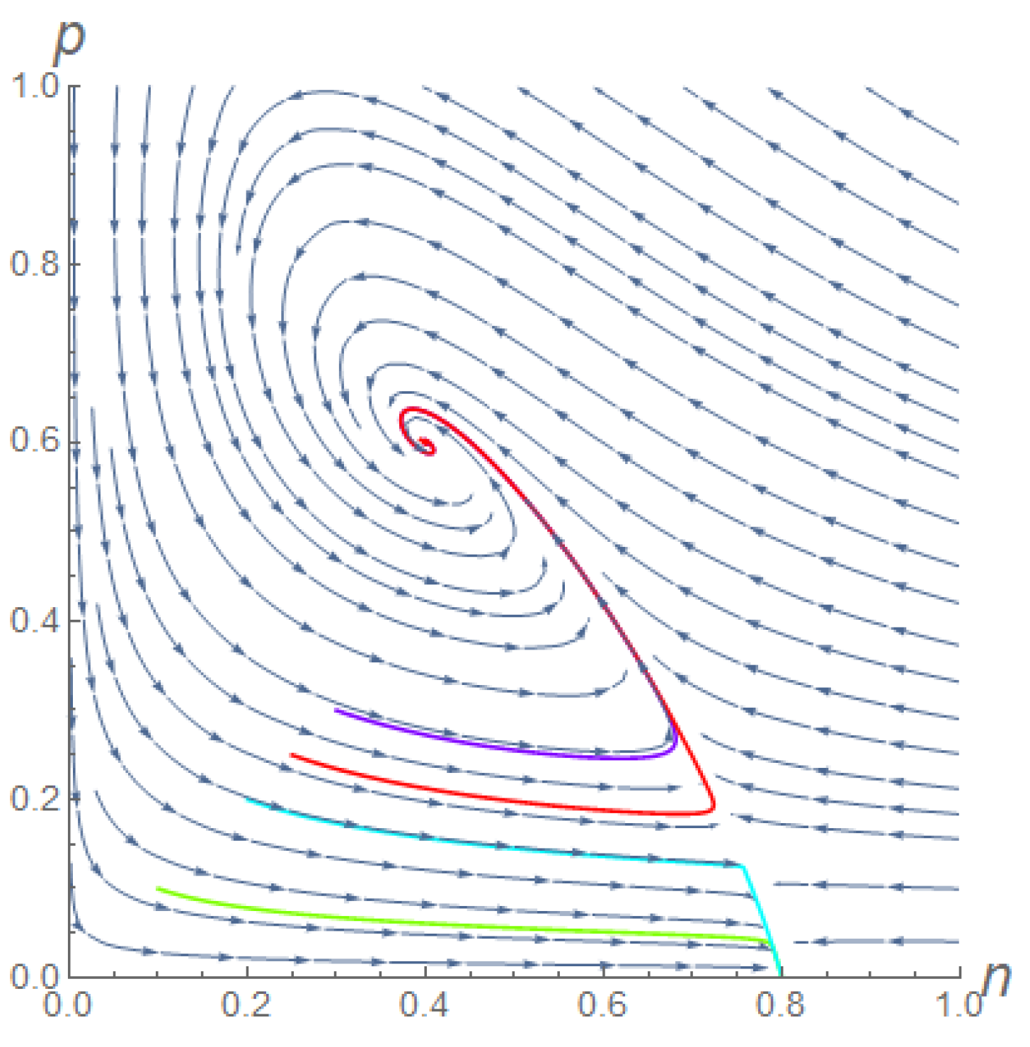
When $K<1$, the boundary equilibrium $E_1$ was always stable. Therefore, two coexistent equilibria could exist when conditions (5) were met. One (or both) of them could be stable provided that the conditions (6), given in Theorem 1, were met. Figure 1 shows a phase portrait of this situation, where orbits could reach the boundary steady state $E_1$ or the stable coexistent equilibrium $E^{*}$, depending on their starting point.

For the traveling wave solutions of (9), the situation was more complex and, therefore, more complicated. In the following, we examine all scenarios in detail. To simplify the description and interpretation of the different cases, we chose to consider one dimension in space, so that $x,\kappa ,v_1,v_2$ were all scalar quantities. Moreover, we scaled $\kappa$ to 1. In this setting, $v_1$ and $v_2$ represented the average individual speed for a prey and a predator, respectively, to be compared with the band speed c.

4.1. $K>1$

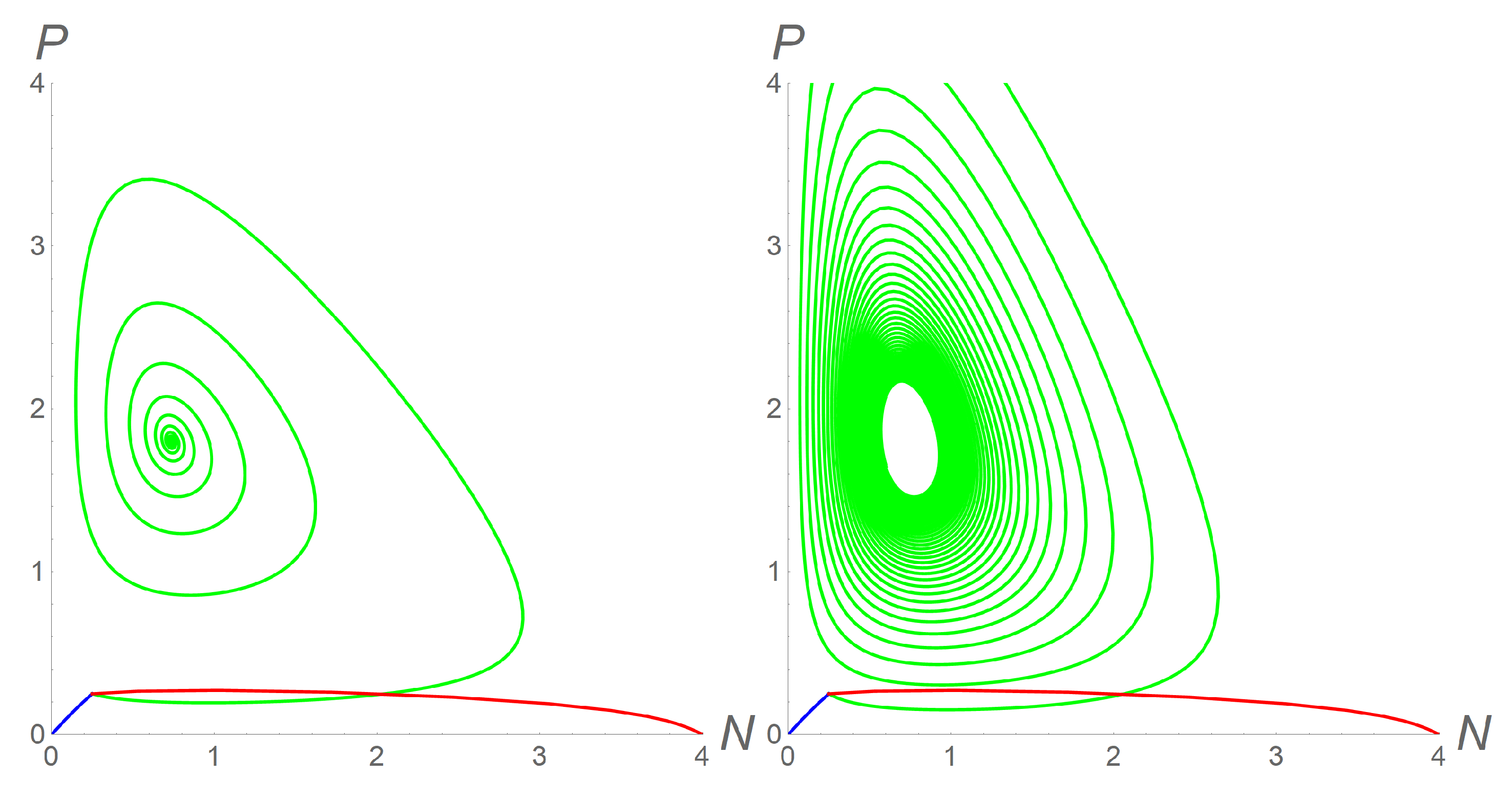
Once we fixed the values of the model parameters $\sigma ,\alpha ,$ and K, we could still observe changes in the stability of all the equilibria, as stated in Theorem 2, according to different values of $c,v_1,\mathrm{and}{v}_2$. Specifically, we chose $\sigma$ = 3, $\alpha$ = 0.2 (corresponding to a weak cooperation among predators), and K = 4. Then for all the simulations, we fixed the same initial conditions ${\mathcal{N}}_0$ = ${\mathcal{P}}_0$ = 0.25. All results for this case are shown in the left panel of Figure 2. First, we chose c = 2, and $v_1$ = $v_2$ = 1. In this case, system (12) formally reduced to (2), so that the only coexistent equilibrium was $E^{*}\approx$ (0.74; 1.80). In this case, the constants $\overline{\sigma }$ and ${\sigma }^{*}$ had the approximate values 1.4 and 60, respectively, so that conditions (6) were met. Then, $E^{*}$ was stable, and the orbit in the phase plane starting from (0.25; 0.25) approached it (green line). Therefore, we fixed c = 0.2, $v_1$ = 0.5, and $v_2$ = 0.1, to describe a scenario where the bands of prey moved slowly while the bands of predators moved quickly, consequently increasing the predatory pressure. Predators would greedily hunt all prey, consume them, and consequently go extinct themselves. As stated in Theorem 2, the only stable equilibrium was $E_0$, so that both populations would go extinct (blue line). Finally, if we chose c = 0.2, $v_1$ = 0.1, and $v_2$ = 0.5, so that the bands of prey moved quickly, while the bands of predators moved slowly, the only stable equilibrium was $E_1$: predators would go extinct, and prey density would reach the saturated value K (red line). In addition, we found that even in the first described case ($c>v_1$ and $c>v_2$) with the coexistent equilibrium $E^{*}$ verifying the requirement (6), an imbalance between the individual velocities $v_1$ and $v_2$ could lead to instability, confirmed by the appearance of a limit cycle in the phase portrait. Indeed, by modifying only the value $v_2$ = 1.5 according to the first example (with c = 2, $v_1$ = 1), the green orbit leading to the coexistence of a steady state, as shown in the left panel of Figure 2, transformed into the one shown in the right panel of the same figure.

4.2. $K<1$ and No Coexistent Equilibrium Exists

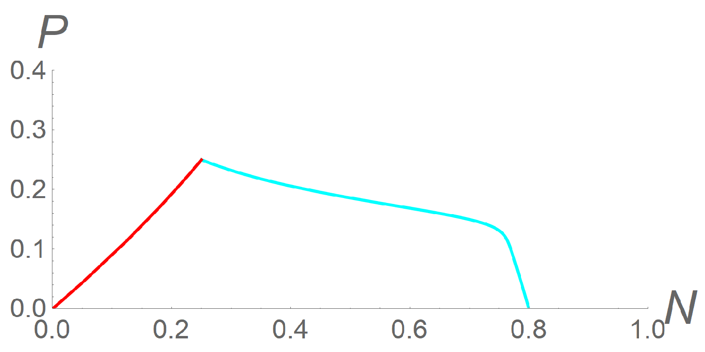
In this case, a suitable choice of the velocities could lead to the extinction of both populations ($E_0$ became stable and $E_1$, unstable). To represent this situation, we fixed the values of the model parameters as $\sigma$ = 3, $\alpha$ = 0.6 (corresponding to a weak cooperation among predators), and K = 0.8. Again, we fixed as initial conditions ${\mathcal{N}}_0$ = ${\mathcal{P}}_0$ = 0.25. All results for this case are shown in Figure 3. Therefore, if we choose c = 2 and $v_1$ = $v_2$ = 1, system (12) again reduced to (2), so that the only stable equilibrium was $E_1$ = (0.8; 0): predators would go extinct while density of prey would reach its maximum possible value (pale blue line). However, if we chose, instead, c = 0.2, $v_1$ = 0.5, and $v_2$ = 0.1, $E_1$ lost its stability, and the only stable equilibrium was $E_0$, so that both populations would go extinct (red line). This choice of parameters represented a situation in which either the prey population was not very sensitive to predatory pressure or not sufficiently interested in its own safety, and then the bands of prey would move slowly; or the bands of hungry predators moved fast and captured all the prey, and all would become extinct.

4.3. $K<1$ and Two Coexistent Equilibria Exist

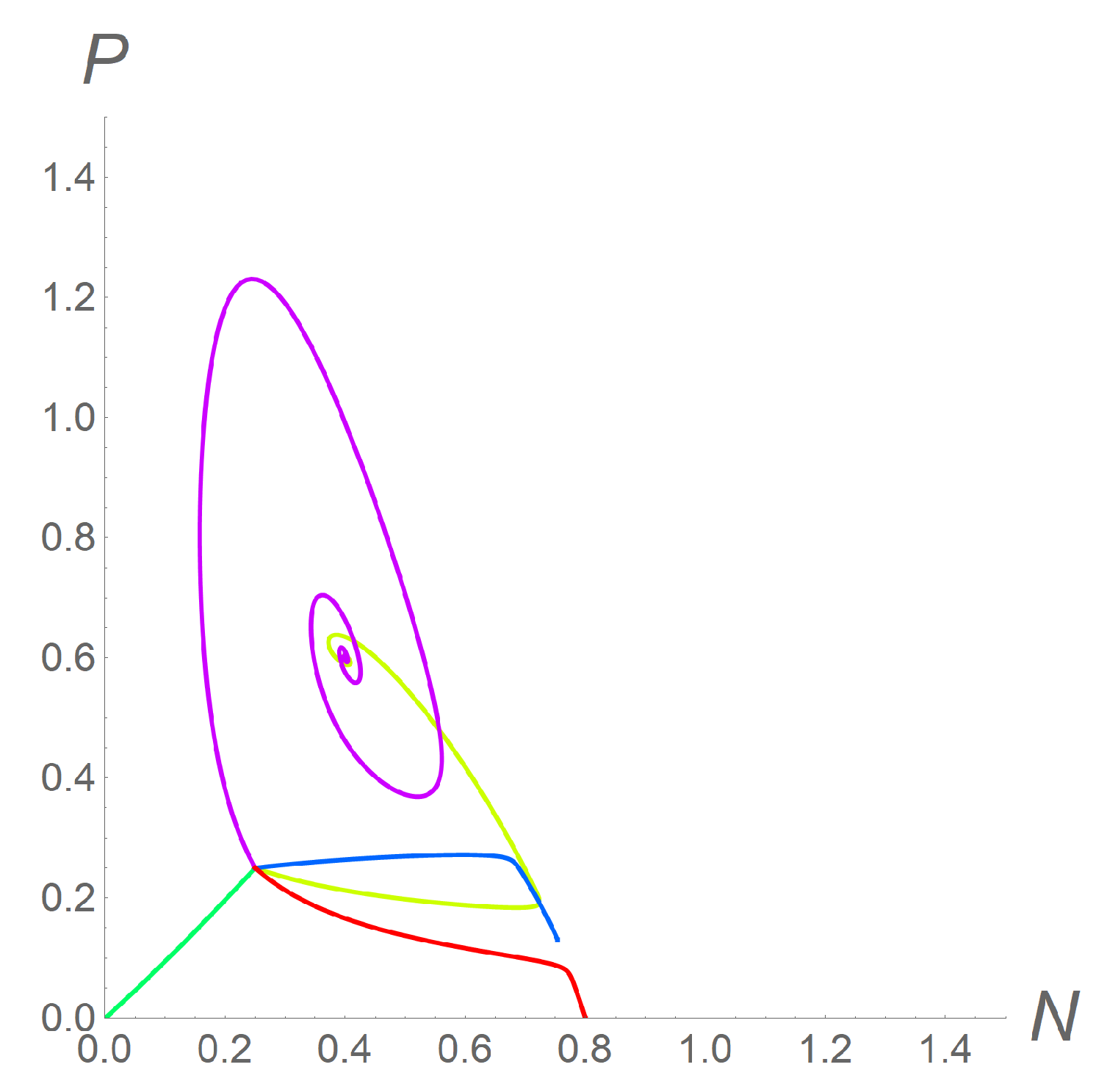
This situation was undoubtedly the most complex, as compared to the other scenarios. We could observe the stability of each one of the equilibria and also the coexistence of two different stable steady states, so that orbits could reach any one of them, according to different initial conditions. As an example, we chose again the model parameters as $\sigma$ = 3 and K = 0.8 while $\alpha$ = 2.5 (corresponding to a strong cooperation among predators). In this case, system (2) admitted two coexistent equilibria, $E_1^{*}\approx$ (0.75; 0.13) and $E_2^{*}\approx$ (0.4; 0.6). For $E_1^{*}$, the constants ${\overline{\sigma }}_1$ and ${\sigma }_1^{*}$ had the approximate values 0.26 and 0.93, respectively, so that the conditions (6) were not met: $E_1^{*}$ was an unstable steady state for system (2). On the contrary, $E_2^{*}$ was a stable steady state for system (2), since the approximate values of the constants ${\overline{\sigma }}_2$ and ${\sigma }_2^{*}$ were 1.2 and 8.0, respectively. As a consequence, if we chose c = 2 and $v_1$ = $v_2$ = 1, so that system (12) reduced to (2), the orbit reached the stable equilibrium $E_2^{*}$ or, as shown in Figure 1, the boundary equilibrium $E_1$, depending on the chosen initial conditions. Figure 4 shows the phase portrait corresponding to this parameter setting, with orbits always starting from ${\mathcal{N}}_0$ = ${\mathcal{P}}_0$ = 0.25: the yellow line ends in $E_2^{*}$.

A different setting for the velocities, as in the previous examples (c = 0.2, $v_1$ = 0.5, $v_2$ = 0.1), led to a situation where $E_0$ was the only stable equilibrium and both populations would go extinct (green line). As a third setting, we chose c = 0.2, $v_1$ = 0.1, and $v_2$ = 0.5. Then, $E_1$ lost its stability, and the orbit approached the first coexistent equilibrium $E_1^{*}$ (blue line). Convergence of the orbit towards $E_2^{*}$ was also possible when $c<v_1$ and $c<v_2$: indeed, for c = 0.1, $v_1$ = 0.6, and $v_2$ = 0.2, $E_2^{*}$ was the only stable steady state (magenta line). Finally, when c = 0.6, $v_1$ = 0.1, and $v_2$ = 0.4, none of the coexistent equilibria were stable, and the orbit reached the boundary equilibrium $E_1$ (red line).

5. Conclusions

Spatial effects are often relevant in interacting population dynamics. Among them, models involving convective pursuit and evasion have been particularly significant for ecological studies, but they are also challenging. From this perspective, the present study considered a generalization of a predator–prey model with the logistical growth of the prey and the hunting cooperation of predators by the inclusion of suitable terms representing the species’ movements. A traveling waves analysis allowed us to characterize the interplay between the aggregated movements of bands of both populations and the individual velocities. Theoretical results on the stability of the traveling bands equilibria, also as comparison to the model without advective terms, were obtained. Such results were confirmed by specific numerical simulations. Future work will include the analysis and numerical simulation of a diffusive advection system to assess the combined effect of directed movement and random dispersion on the model dynamics. Different choices, such as a single species diffusion, both species dispersion, and even cross-diffusion should be considered. In these extended spatial models, the shape of the domain should also be considered in order to represent more complex ecosystems.

References

- Courchamp, F.; Berec, L.; Gascoigne, J. Allee Effects in Ecology and Conservation; Oxford University Press: Oxford, UK, 2008. [Google Scholar]
- Teixeira Alves, M.; Hilker, F.M. Hunting cooperation and Allee effects in predators. J. Theor. Biol. 2017, 419, 13–22. [Google Scholar] [CrossRef]
- Cantrell, R.S.; Cosner, C. Spatial Ecology via Reaction-Diffusion Equations; John Wiley and Sons Ltd.: Hoboken, NJ, USA, 2003. [Google Scholar]
- Murray, J. Mathematical Biology I. An Introduction; Springer: New York, NY, USA, 2002; Volume 17. [Google Scholar]
- Murray, J. Mathematical Biology II. Spatial Models and Biomedical Applications; Springer: New York, NY, USA, 2003; Volume 18. [Google Scholar]
- Okubo, A. Diffusion and Ecological Problems: Mathematical Models; Springer: New York, NY, USA, 1980. [Google Scholar]
- Prigogine, I.; Lefever, R. Symmetry breaking instabilities in dissipative systems. II. J. Chem. Phys. 1968, 48, 1698–1700. [Google Scholar] [CrossRef]
- Rionero, S.; Torcicollo, I. On the dynamics of a nonlinear reaction-diffusion duopoly model. Int. J. Non-Linear Mech. 2018, 99, 105–111. [Google Scholar] [CrossRef]
- Torcicollo, I. On the dynamics of a non-linear Duopoly game model. Int. J. Non-Linear Mech. 2013, 57, 31–38. [Google Scholar] [CrossRef]
- Mishra, S.; Upadhyay, R.K. Strategies for the existence of spatial patterns in predator–prey communities generated by cross-diffusion. Nonlinear Anal. Real World Appl. 2020, 51, 103018. [Google Scholar] [CrossRef]
- Torcicollo, I. On the nonlinear stability of a continuous duopoly model with constant conjectural variation. Int. J. Non-Linear Mech. 2016, 81, 268–273. [Google Scholar] [CrossRef] [Green Version]
- Abundo, M.; Ascione, G.; Carfora, M.F.; Pirozzi, E. A fractional PDE for first passage time of time-changed Brownian motion and its numerical solution. Appl. Numer. Math. 2020, 155, 103–118. [Google Scholar] [CrossRef]
- Carfora, M.F.; Torcicollo, I. Identification of epidemiological models: The case study of Yemen cholera outbreak. Appl. Anal. 2020, 101, 3744–3754. [Google Scholar] [CrossRef]
- Capone, F.; Carfora, M.F.; De Luca, R.; Torcicollo, I. Turing patterns in a reaction-diffusion system modeling hunting cooperation. Math Comput. Simul. 2019, 165, 172–180. [Google Scholar] [CrossRef]
- Capone, F.; Carfora, M.F.; Luca, R.D.; Torcicollo, I. Nonlinear stability and numerical simulations for a reaction—Diffusion system modelling Allee effect on predators. Int. J. Nonlinear Sci. Numer. Simul. 2021, 000010151520200015. [Google Scholar] [CrossRef]
- Carfora, M.; Torcicollo, I. Cross-diffusion-driven instability in a predator–prey system with fear and group defense. Mathematics 2020, 8, 1244. [Google Scholar] [CrossRef]
- Odell, G.M. Biological waves. In Mathematical Models in Molecular and Cellular Biology; Segel, L.A., Ed.; Cambridge University Press: Cambridge, UK, 1980. [Google Scholar]
- Hori, Y.; Miyazako, H. Analysing diffusion and flow-driven instability using semidefinite programming. J. R. Soc. Interface 2019, 16, 20180586. [Google Scholar] [CrossRef] [PubMed] [Green Version]
- Ibrahim, H.; Nasreddine, E. Traveling waves for a model of individual clustering with logistic growth rate. J. Math. Phys. 2017, 58, 081505. [Google Scholar] [CrossRef]
- Zhang, T.; Jin, Y. Traveling waves for a reaction—Diffusion–advection predator–prey model. Nonlinear Anal. Real World Appl. 2017, 36, 203–232. [Google Scholar] [CrossRef]
- Liang, D.; Wu, J. Travelling Waves and Numerical Approximations in a Reaction Advection Diffusion Equation with Nonlocal Delayed Effects. J. Nonlinear Sci. 2003, 13, 289–310. [Google Scholar] [CrossRef]
- Tchepmo Djomegni, P.; Govinder, K.S.; Doungmo Goufo, E.F. Movement, competition and pattern formation in a two prey-one predator food chain model. Comp. Appl. Math. 2017, 37, 2445–2459. [Google Scholar] [CrossRef]
- Di Costanzo, E.; Ingangi, V.; Angelini, C.; Carfora, M.F.; Carriero, M.; Natalini, R. A Macroscopic Mathematical Model for Cell Migration Assays Using a Real-Time Cell Analysis. PLoS ONE 2016, 11, e0162553. [Google Scholar] [CrossRef]
- Tchepmo Djomegni, P.; Duffy, K. Multi-dynamics of travelling bands and pattern formation in a predator–prey model with cubic growth. Adv. Differ. Equ. 2016, 2016, 265. [Google Scholar] [CrossRef] [Green Version]
- Sumpter, D.J. The principles of collective animal behavior. Philos. Trans. R. Soc. Biol. Sci. 2006, 361, 4–22. [Google Scholar] [CrossRef]
- Perc, M.; Gomez-Gardenes, J.; Szolnoki, A.; Flora, L.; Moreno, Y. Evolutionary dynamics of group interactions on structured populations: A review. J. R. Soc. Interface 2013, 10, 20120997. [Google Scholar] [CrossRef] [Green Version]
- Perc, M.; Gomez-Gardenes, J.; Szolnoki, A.; Flora, L.; Moreno, Y. Evolutionary game thery: Theoretical concepts and applications to microbial communities. Physica A 2010, 389, 4265–4298. [Google Scholar] [CrossRef] [Green Version]
- Franz, B.; Xue, C.; Painter, K.; Erban, R. Traveling waves in hybrid chemotaxis models. Bull. Math. Biol. 2014, 76, 377–400. [Google Scholar] [CrossRef] [PubMed] [Green Version]
- Landaman, K.; Cai, A.; Hughes, B. Travelling waves of attached and detached cells in a wound-healing cell migration assay. Bull. Math. Biol. 2007, 69, 2119–2138. [Google Scholar] [CrossRef] [PubMed]
- Edelstein-Keshet, L.; Watmough, J.; Grunbaum, D. Do travelling band solutions describe cohesive swarms? An investigation for migratory locusts. J. Math. Biol. 1998, 36, 515–549. [Google Scholar] [CrossRef]
- Song, D.; Li, C.; Song, Y. Stability and cross-diffusion-driven instability in a diffusive predator–prey system with hunting cooperation functional response. Nonlinear Anal. Real World Appl. 2020, 54, 103106. [Google Scholar] [CrossRef]
- Carfora, F.; Torcicollo, I. A Fractional-in-Time Prey–Predator Model with Hunting Cooperation: Qualitative Analysis, Stability and Numerical Approximations. Axioms 2021, 10, 78. [Google Scholar] [CrossRef]
- Ghimire, S.; Wang, X. Traveling waves in cooperative predation: Relaxation of sublinearity. Math. Appl. Sci. Eng. 2021, 2, 22–31. [Google Scholar] [CrossRef]
- Merkin, D. Introduction to the Theory of Stability; Springer: Berlin/Heidelberg, Germany, 1997; Volume 24. [Google Scholar]
- Mathematica; Version 11.3.0; Wolfram Research, Inc.: Champaign, IL, USA, 2018.
Figure 1.
Phase portrait of the orbits of system (2) in the case : once fixed K = 0.8, = 2.5, = 3, both (0.8, 0) and (0.4, 0.6) are stable. Then, different starting points lead to different steady states. Here, for (, ) = (0.1, 0.1) and (, ) = (0.2, 0.2), the orbits reach (green and pale blue lines, respectively), while for (, ) = (0.25, 0.25) and (, ) = (0.3, 0.3), the orbits reach (red and violet lines, respectively). The superimposed stream plot highlights the basins of attraction of the two equilibria.
Figure 2.
Phase portrait for system (9) in the case . The parameters are fixed as = 3, = 0.2, and K = 4, and the initial conditions as = = 0.25 for all simulations. In both panels, the settings c = 0.2, = 0.5, and = 0.1 leads the orbit towards (blue line) and the settings c = 0.2, = 0.1, and = 0.5 leads the orbit towards (red line). In the left panel, the settings c = 2, and = = 1 leads the orbit towards (green line); in the right panel, with c = 2, = 1, and = 1.5, a limit circle around appears (green line).
Figure 3.
Phase portrait for system (9) in the case , when no coexistent equilibria exist. The parameters are fixed as = 3, = 0.6, and K = 0.8, and the initial conditions as = = 0.25 for all simulations. Now, the setting c = 2 and = = 1 leads the orbit towards (pale blue line), while the setting c = 0.2, = 0.5, and = 0.1 leads the orbit towards (red line).
Figure 4.
Phase portrait for system (9) in the case , when two coexistent equilibria exist. The parameters are fixed as = 3, = 2.5, and K = 0.8, and the initial conditions as = = 0.25, for all simulations. The settings c = 2 and = = 1 (yellow line) as well as c = 0.1, = 0.6, and = 0.2 (magenta line) both lead the orbit towards . The settings c = 0.2, = 0.1, and = 0.5 lead the orbit towards (blue line). With c = 0.2, = 0.5, and = 0.1, the orbit reaches (green line), while the settings c = 0.6, = 0.1, and = 0.4 lead the orbit towards the only stable equilibrium (red line).
Publisher’s Note: MDPI stays neutral with regard to jurisdictional claims in published maps and institutional affiliations. |
© 2022 by the authors. Licensee MDPI, Basel, Switzerland. This article is an open access article distributed under the terms and conditions of the Creative Commons Attribution (CC BY) license (https://creativecommons.org/licenses/by/4.0/).
Share and Cite
MDPI and ACS Style
Carfora, M.F.; Torcicollo, I. Traveling Band Solutions in a System Modeling Hunting Cooperation. Mathematics 2022, 10, 2303. https://0-doi-org.brum.beds.ac.uk/10.3390/math10132303
AMA Style
Carfora MF, Torcicollo I. Traveling Band Solutions in a System Modeling Hunting Cooperation. Mathematics. 2022; 10(13):2303. https://0-doi-org.brum.beds.ac.uk/10.3390/math10132303
Chicago/Turabian StyleCarfora, Maria Francesca, and Isabella Torcicollo. 2022. "Traveling Band Solutions in a System Modeling Hunting Cooperation" Mathematics 10, no. 13: 2303. https://0-doi-org.brum.beds.ac.uk/10.3390/math10132303
Note that from the first issue of 2016, this journal uses article numbers instead of page numbers. See further details here.