A Multi-Start Biased-Randomized Algorithm for the Capacitated Dispersion Problem

Abstract

The capacitated dispersion problem is a variant of the maximum diversity problem in which a set of elements in a network must be determined. These elements might represent, for instance, facilities in a logistics network or transmission devices in a telecommunication network. Usually, it is considered that each element is limited in its servicing capacity. Hence, given a set of possible locations, the capacitated dispersion problem consists of selecting a subset that maximizes the minimum distance between any pair of elements while reaching an aggregated servicing capacity. Since this servicing capacity is a highly usual constraint in real-world problems, the capacitated dispersion problem is often a more realistic approach than is the traditional maximum diversity problem. Given that the capacitated dispersion problem is an NP-hard problem, whenever large-sized instances are considered, we need to use heuristic-based algorithms to obtain high-quality solutions in reasonable computational times. Accordingly, this work proposes a multi-start biased-randomized algorithm to efficiently solve the capacitated dispersion problem. A series of computational experiments is conducted employing small-, medium-, and large-sized instances. Our results are compared with the best-known solutions reported in the literature, some of which have been proven to be optimal. Our proposed approach is proven to be highly competitive, as it achieves either optimal or near-optimal solutions and outperforms the non-optimal best-known solutions in many cases. Finally, a sensitive analysis considering different levels of the minimum aggregate capacity is performed as well to complete our study.

1. Introduction

The capacity limitation of a facility is a typical constraint in supply networks. A production plant or a distribution center can manufacture or manage only a limited quantity of product in a given time. Highly cited reviews [1,2] affirm that determining the capacities of facilities is one of the most common strategic decisions in the supply chain network design topic. According to Correia and Saldanha-da Gama [3], the operating capacity is a decision that must be made even before knowing the demand. Additionally, one of the biggest difficulties posed whenever a facility must be located is considering that its capacity is insufficient to satisfy customer demand [4]. That is, the capacity of the active facilities must be ideally greater than the total demand that must be serviced. This condition appears in most logistics challenges at any decision level (strategic, tactical, and operational).

One example of a strategic logistics challenge is the well-known facility location problem (FLP) [5,6,7,8,9], which consists of locating a set of facilities with the objective of minimizing both the setup costs and the cost of servicing a set of customers from the facilities. The FLP can be capacitated [10] or uncapacitated [11], depending on whether the facilities have a restricted capacity or one that exceeds any possible demand from the customers. Some FLP versions include a location-allocation problem, i.e., we must decide not only which facilities should be open (location) but also how to assign the customers to each open facility (allocation). Similar challenges also appear in other types of networks, such as telecommunication ones, where ‘facilities’ refer to communication devices and ‘capacity’ refers to the volume of data they can transmit at a given quality of service level [12].

Maximum diversity problems (MDP) are another family of related facility optimization problems that are less explored by the literature [13]. They do not include the allocation part of the FLP but only the location component. Additionally, typical objective functions in these diversity problems do not seek to minimize cost but to optimize indicators regarding the distances among the open facilities [14]. Furthermore, diversity problems can also be employed to model situations where a subset of elements must be selected from a given set, and distances between the elements in the subset must be minimized.

Hence, fields as different as workforce selection, gender diversity, medical treatment, capital investment, telecommunication services, pollution control, or environmental balance [13,15] show the broad application of MDP. Most of the published literature on diversity problems considers that the number of best elements to select (or facilities to open) is determined according to an initially defined criterion for the problem. The selection objective must effectively represent the diversity existing in the original collection of possibilities, i.e., the selection must guarantee that a function reaches a maximum or minimum in the combinatorial optimization problem.

Model (1) is an example of a typical integer program that represents a diversity problem with the objective of maximizing the minimum distance between any pair of selected elements (active facilities) [16]. In this model, V is the set of elements, $d_{ij}$ is the distance between elements $i\in V$ and $j\in V$, p is the number of elements to be selected, and $x_i$ is a binary variable that takes the value 1 if element $i\in V$ is selected and 0 otherwise.

$$\begin{array}{cccc}\hfill & \hfill & \hfill max& \underset{\begin{array}{c}i,j\in V\\ i<j\end{array}}{\min }\{d_{ij}:x_i{x}_j=1\}\hfill \\ \hfill & \hfill & \hfill s.t.& \sum _{i\in V}{x}_i=p\hfill \\ \hfill & \hfill & \hfill & x_i\in \{0,1\}\forall i\in V\hfill \end{array}$$

(1)

Despite that models similar to Model (1) are widely used to represent diversity problems, they are often not practical in some strategic logistics situations, where the minimum servicing capacity must be included as a threshold. Selecting a known number of p facilities (selected elements) does not guarantee that the demand is satisfied, since each facility may have a different capacity depending on their location, market conditions, etc. [17,18]. Hence, sometimes we need to consider a minimum capacity to meet, i.e., the aggregate capacity of the open facilities must not be less than a given threshold. Consequently, we address a capacitated dispersion problem (CDP) [19], which has the same objective function as Model (1)—i.e., to maximize the dispersion of the open facilities—but fixing a given capacity threshold instead of considering a given number of facilities, p.

These characteristics can be observed in multiple real-world situations, e.g., (i) determining the location of undesirable facilities, such as landfills or nuclear reactors [20]; (ii) location problems where the objective is to reach a population as large as possible to increase the service level, such as hospitals or schools [21], and (iii) setting the location of franchise outlets that should be as far as possible from each other to avoid competition between them [22].

In this context, Lozano-Osorio et al. [23] showed a case study in which a real-world application of the CDP was addressed. These authors not only considered a capacity restriction but also a budget constraint. The CDP has been proven to be NP-hard [24], which implies that exact methods might require a vast amount of time to guarantee optimality of a solution when coping with large-sized instances. Hence, finding high-quality or near-optimal solutions in a short computational times requires the use of approximate methods, such as metaheuristics.

Consequently, the main contribution of this work is to propose a biased-randomized algorithm [25,26] that uses a construction–destruction logic to generate high-quality solutions for the CDP in short computing times. In order to do so, the algorithm also makes use of a multi-start schema and a local search strategy. Our approach can be seen as an extension to the CDP of the destructive approaches proposed for the non-restricted MDP by Glover et al. [15] and Duarte and Martí [27].

In addition, our algorithm also incorporates biased-randomization techniques, which contribute to enhance the searching process. The remainder of the paper is organized as follows: Section 2 revises some related work on diversity problems. Section 3 provides a detailed description of the problem we are addressing, as well as an integer non-linear model for the CDP. Section 4 describes the biased-randomized algorithm proposed to solve this problem. Section 5 shows the numerical results obtained after testing our procedures. They are compared with previously published results. Finally, Section 6 outlines some general concluding remarks and future research lines.

2. Related Work on Diversity Problems

Some early studies addressing diversity problems can be found in the scientific literature [15,28,29,30]. More recently, Sandoya et al. [14] performed a review of different diversity, dispersion, and equity models, as well as the metaheuristics employed in solving them. They performed a correlation analysis to identify similarities and differences between these problems. Five models were identified:

• The Max-Min problem, whose objective is to maximize the minimum distance between any pair of elements in a solution.
• The Max-Sum problem, whose objective is to maximize the total distance among all elements in a solution.
• The Max-Mean problem, whose objective is to maximize the average dispersion of the elements, while the remaining problems in this list set a predefined number of elements, the Max-Mean problem does not require this constraint.
• The Max-MinSum problem, whose objective is to maximize the minimum aggregate dispersion of each element in a solution.
• The Min-Diff problem, whose objective is to minimize the difference between the maximum and the minimum aggregate dispersion of each element in a solution.

Problems 1 and 2 seek to optimize efficiency. Conversely, problems 3, 4, and 5 were proposed by Prokopyev et al. [31] with the objective of maximizing equity. These authors formulated each problem as a mathematical programming model. Equivalent linear models were formulated as well. Both exact and approximate methods were employed by the authors to solve the aforementioned problems. Additionally, Parreno et al. [32] performed a thorough comparison between models 1, 2, 4, and 5. These authors presented mathematical formulations for each of these problems, which were later solved by utilizing the commercial CPLEX solver. Both numerical and geometrical results were analyzed.

Finally, the authors proposed a new mathematical model to achieve diversity. The most recent review article on diversity, dispersion, and equity models was performed by Martí et al. [13], who showed how these problems have evolved over time from an Operations Research perspective. New benchmark instances were proposed and tested through a series of computational experiments.

Perhaps the Max-Sum problem is the most-addressed diversity model in the literature. For instance, Duarte and Martí [27] compared memory-based procedures, inspired by tabu search (TS), with memory-less ones based on GRASP. The authors concluded that algorithms employing memory tended to yield higher quality results. Martí et al. [33] performed a thorough comparison of different heuristics and metaheuristics to solve the Max-Sum diversity problem. Both benchmark and newly-introduced instances were used to test these approaches. These authors showed that, in general, local search based metaheuristics, such as the variable neighborhood search (VNS), provide excellent results.

Alternatively, Martí et al. [34] proposed an exact algorithm based on the branch-and-bound method to solve this problem. Moreover, a group of upper bounds was calculated for partial solutions. Additional algorithms can be found in the literature about the Max-Sum problem, such as an iterated greedy metaheuristic [35], an opposition-based memetic algorithm [36], or the comparison of an exploring TS, a scatter search, a VNS, and a simple random restart algorithm [37].

Literature about the Min-Diff dispersion problem includes the work by Mladenović et al. [38], who proposed a VNS metaheuristic to solve it. The proposed algorithm yielded new best-known solutions (BKS) for 170 out of 190 benchmark instances. The same problem was addressed by Duarte et al. [39], who proposed a set of hybrid algorithms that combine GRASP, VNS, and path relinking. The results were compared with both previously published metaheuristics and optimal results yielded by CPLEX. Other approaches have been proposed to solve this problem, such as a hybridization between TS and memetic search [40], iterated local search [41], or an intensification-driven TS [42].

Regarding the Max-Mean dispersion problem, Martí and Sandoya [43] proposed a hybridization between GRASP, path relinking, and variable neighborhood descent (VND) to solve it. Their results were compared with alternative state-of-the-art methods. Additional algorithms addressing the Max-Mean problem can be found in the literature, such as a TS-based memetic algorithm [44], a dynamic TS [45], or a VNS [46]. Finally, the Max-MinSum dispersion problem has been studied as well.

For instance, Lai et al. [47] solved this problem through a solution-based TS algorithm. The obtained results show that this approach outperformed the BKS for 80 out of 140 benchmark instances. Other approaches employed to solve this problem have been a VNS [48], a TS and a GRASP [49], or a TS with a dynamical neighborhood size [50].

Studies on the CDP have traditionally used the Max-Min model as an objective function. Rosenkrantz et al. [24] introduced this problem from a theoretical point of view. Since then, only a few published articles have studied the CDP. Accordingly, the related literature is scarce as compared with other dispersion problems. In fact, the traditional “uncapacitated” Max-Min problem has been more thoroughly studied. For instance, Resende et al. [16] hybridized GRASP and different variants of path relinking to solve it. The results were compared with the ones obtained from previous algorithms found in the literature.

To the best of our knowledge, only a few published articles have addressed the CDP. In Peiró et al. [19], the authors proposed a hybrid heuristic combining the GRASP and VND metaheuristics within a strategic oscillation approach to solve it. The problem was initially modeled using a mixed-integer linear program (MILP). The proposed model is an adaptation of the model formulated by Kuo et al. [29]. A set of benchmark instances were used to compare the results yielded by both the exact and the metaheuristic approaches. Additionally, Martí et al. [51] also proposed both an exact and a heuristic approach to solve the CDP.

First, the authors formulated a new MILP model based on the work by Sayyady and Fathi [52]. Then, a heuristic based on the scatter search methodology is presented. Both approaches yielded results that outperformed the ones reported in previous works, both in terms of quality of the final solution as well as computational times. Finally, Martínez-Gavara et al. [21] extended the CDP by proposing the so-called generalized dispersion problem, which not only includes the capacity constraint but also a maximum budget that cannot be exceeded. The GRASP and LS metaheuristics were proposed to solve this problem. A set of small-, medium-, and large-sized benchmark instances was used to test the proposed approaches.

3. Problem Definition

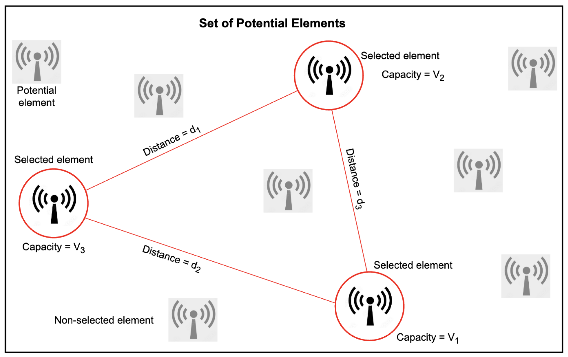
The problem addressed in this article is a CDP in which the objective function employs the Max-Min model. In order to provide an intuitive view of of the problem studied, and without loss of generality, we will assume that the considered elements are facilities to open in a logistics network. Therefore, given a set of potential facilities, the problem consists of selecting a subset such that the minimum distance between any pair of open facilities is maximized. Unlike the traditional Max-Min diversity problem, the number of facilities to open in this problem is not given as an input parameter.

Instead, each facility has a known capacity, and the aggregated capacity of the open facilities must be above a given user-defined threshold. Figure 1 depicts a small example of a final solution to the problem addressed, where a set of potential elements (telecommunication devices in this case) is considered. Each element might have a different capacity in terms of the volume of data it can efficiently transmit above a given quality of service level. Selected elements in the solution are surrounded with a circle, and the distances among them have been drawn.

In a more formal way, the CDP can be defined on a complete, weighted, and undirected graph $G(V,E)$, in which V is the set of facilities, and E is the set of edges connecting these facilities. If $i,j\in V$, with $i\ne j$, each edge $(i,j)\in E$ has a distance $d_{ij}>0$ that satisfies the triangle inequality. All distances are symmetric, i.e., $d_{ij}=d_{ji}$. Each facility $i\in V$ has a known deterministic capacity $c_i>0$. An aggregated servicing capacity b is required as a threshold. Then, the CDP consists of finding a subset $O\subset V$ of facilities to open, with aggregated capacity exceeding b and such that the minimum distance between any pair of facilities $i,j\in S$ is maximized. In this context, $x_i$ is a binary variable that takes the value 1 if facility $i\in V$ is included in O and 0 otherwise. Then, an integer programming model for this problem can be formulated as follows:

$$Maximize\underset{\begin{array}{c}i,j\in O\\ i<j\end{array}}{\min }{d}_{ij}$$

(2)

$$s.t.\sum _{i\in V}{c}_i{x}_i\ge b$$

(3)

$$x_i\in \{0,1\}\forall i\in V$$

(4)

The objective function (2) maximizes the minimum distance between any pair of open facilities. Constraint (3) guarantees that the minimum required capacity is met. Finally, constraint (4) defines the values that decision variables can take. This model can be linearized, as shown by Peiró et al. [19] and Martí et al. [51].

4. Solution Approaches for the Capacitated Dispersion Problem

Since the problem described in Section 3 is NP-hard, two different approximate methods to solve it are proposed. The proposed approaches make use of biased-randomization techniques [53], which are also combined with local search strategies within a multi-start framework. Biased-randomized techniques propose the use of a skewed probability distribution in order to induce an oriented (biased) random behavior in a constructive heuristic, thus, transforming a deterministic procedure into a probabilistic algorithm while maintaining the logic behind the heuristic [54].

This type of algorithm is highly flexible and can be designed to work with a reduced set of parameters, which diminishes the need to perform time-consuming fine-tuning processes and enhances their applicability in real-life. The first proposed heuristic is based on a “constructive” strategy. It starts with all facilities closed and then iteratively opens new facilities (one at a time) until the required capacity is met, i.e., until the solution becomes feasible.

The second heuristic follows a “destructive” strategy: it starts with all facilities open—which makes the solution feasible from the very beginning—and then iteratively removes facilities (one at a time) while the solution is still feasible. Notice that these two heuristics are complementary, and therefore they can be executed in parallel. Depending on the specific instance being analyzed, one will tend to perform better than the other, e.g., in instances in which the optimal value is reached when most of the facilities are open, the destructive strategy might be more efficient, and vice versa. Hence, after a fast comparison, we can choose the one that better adapts to the instance and then extend it into a full multi-start biased-randomized algorithm, which might also include a local search and other advanced features.

4.1. A Constructive Heuristic

Algorithm 1 shows the main procedure of the constructive heuristic, which extends the algorithm proposed by Martí et al. [51]. This approach generates a feasible initial solution (S). It starts from a hypothetical scenario where all facilities are initially closed, i.e., the algorithm starts with an empty initial solution (line 1). Then, the list of edges ($edge\_list$), which contains the set of edges connecting each pair of facilities, is decreasingly sorted according to the computed distance (line 2), i.e., it is ordered starting with the pair of facilities with the longest distance between them, and ending with the pair of facilities with the shortest distance between them. Next, the algorithm selects the element at the top position of $edge\_list$ (line 3).

Subsequently, the pair of facilities that compose the selected edge are included in the solution (line 4). Later, the objective function f is computed for the first time, considering the distance between these two facilities (line 5). The heuristic generates a preference list of candidate facilities ($node\_list$) to be included in the solution in order to decide the most suitable ones to add in each iteration. Thus, for each unselected facility, the algorithm calculates the distance with respect to all the facilities within the solution and then creates an edge connecting the unselected facility with the one in the solution containing the minimum distance between them.

In each new iteration, it is not necessary to re-generate the complete list but only a partially recalculated one. This is done by considering the new facility added in the previous iteration. Next, in order to sort the list, a cost function is implemented. It considers both the calculated distance from the new facility ($distance\_to\_solution$) to each of the facilities currently selected and the capacity of the unselected candidate facility. The cost associated with each element of the list is defined in Equation (5), where $n_i$ is the non-selected facility i. Notice that $\delta \in (0,1)$ is a tuning parameter, which depends on the heterogeneity of the facilities in terms of the capacity.

To be more specific, in scenarios with heterogeneous facilities, in terms of capacity, $\delta$ will be close to 0. On the contrary, $\delta$ will be close to 1 in scenarios with homogeneous facilities in terms of capacity. Then, the list of facilities is sorted in descending order (line 6). Afterwards, while the minimum required capacity is not met (line 7), the algorithm iteratively adds new facilities to the solution from $node\_list$. Hence, the facility at the top position is added to the solution (line 9). Later, the objective function is updated (line 10). Finally, the $node\_list$ is updated considering the new facility in the solution (line 11). This procedure is repeated until the capacity constraint is met.

$$cost\left(n_i\right)=\delta ·distance\_to\_solution\left(n_i\right)+(1-\delta )·capacity\left(n_i\right)$$

(5)

Algorithm 1 is embedded into a multi-start framework, whose main characteristics are depicted in Algorithm 2. Initially, the algorithm generates a feasible initial solution (S) using the constructive heuristic (Algorithm 1). Next, in a second stage, it aims to improve this initial solution by iteratively exploring the search space. In order to diversify the search, the previously described heuristic is extended into a probabilistic algorithm by implementing a biased randomized algorithm [55]. This algorithm introduces a slight modification in the greedy constructive behavior that provides a certain degree of randomness while maintaining the logic behind the constructive heuristic.

Algorithm 1: Constructive heuristic ($edge\_list$)

1: $S\leftarrow \varnothing$ 2: $edge\_list\leftarrow sort(edge\_list$) 3: Select an element i from $edge\_list$ 4: $S\leftarrow S\cup Nodes(edge\_list(i\left)\right)$ 5: $f\leftarrow dist(edge\_list(i\left)\right)$ 6: $edge\_list\leftarrow Update(edge\_list)$ 7: while$\mathit{not}\_\mathit{feasible}\_\mathit{solution}\left(\mathit{S}\right)$do 8:     Select an element i from $node\_list$ 9:     $S\leftarrow S\cup node\_list\left(i\right)$ 10:   $f\leftarrow Update\_f\left(S\right)$ 11:   $node\_list\leftarrow Update(node\_list)$ 12: end while 13: returnS

Algorithm 2: Multi-start biased-randomized constructive heuristic ($t_{max},beta,edge\_list$)

1: $S\leftarrow ConstructiveHeuristic(edge\_list)$ 2: while$(time\le t_{max})$do 3:     $S_{new}\leftarrow BRConstructiveHeuristic\left(beta\right)$ 4:     $S_{new}^{\prime }\leftarrow LocalSearch\left(S_{new}\right)$ 5:     if $f\left(S_{new}^{\prime }\right)>f\left(S\right)$ then 6:          $S\leftarrow S_{new}^{\prime }$ 7:     end if 8: end while 9: returnS

Thus, a new different solution $S_{new}$ is generated in each iteration. Skewed probability distributions have been used in different optimization problems and are usually combined with an iterated local search framework, to induce an ‘oriented’ (non-uniform) random behavior [56,57]. This process turns a deterministic version of the constructive heuristic into a randomized constructive heuristic whilst preserving most of the selection criterion inside the constructive heuristic. In our case, the biased-randomization process is introduced by employing a Geometric probability distribution with a single parameter $\beta$ ($0<\beta <1$), which controls the relative level of greediness present in the randomized behavior of the algorithm.

When $\beta$ takes values close to 1, the behavior is similar to the deterministic version of the heuristic. Conversely, when $\beta$ takes values close to 0, we approximate the behavior of uniform randomness [58]. This biased behavior was introduced in two different points of Algorithm 1. First is at the very beginning of the heuristic, to select the first edge from the list of edges ($edge\_list$) (line 3), which contains the two first facilities of the solution. Second is during the construction process, to select a new facility from the list of candidate facilities ($node\_list$) (line 8).

Therefore, the elements of the list are rearranged applying a biased-randomized process at each iteration, such that better elements are more likely to be ranked at the top of the list. Unlike the deterministic process, each time a new facility is inserted into the solution, the objective function f does not necessarily have to improve. Consequently, the heuristic must check whether it requires updating. This process allows us to generate different ‘promising’ solutions at each iteration of the multi-start process.

Afterwards, Algorithm 2 starts a local search strategy around the new solution $S_{new}$ to get ($S_{new}^{\prime }$). This procedure is depicted in Algorithm 3. It is based on dropping the oldest facility of the solution and reconstructing a feasible solution using the biased-randomized heuristic. Furthermore, a dropped facility is not considered to generate a new solution until all the oldest facilities—i.e., those that have been added before—have been deleted from the solution.

This step reduces the chances of becoming trapped in a local minimum. The procedure is repeated until a maximum number of iterations without improvement is reached. Finally, each time the cost of the new solution ($S_{new}^{\prime }$) improves, the cost of the best solution found thus far (S) and the latter is updated (line 6). This whole procedure is repeated until a stopping criterion is met, which is based on a maximum execution time ($t_{max}$).

Algorithm 3: Local Search (S)

1: $S^{\prime }\leftarrow S$ 2: $\mathit{noImprovement}\leftarrow 0$ 3: while$\mathit{noImprovement}<\mathit{MaxIter}$do 4:     $\mathit{noImprovement}\leftarrow \mathit{noImprovement}+1$ 5:     $u\leftarrow \mathit{oldest}\_\mathit{selected}\_\mathit{node}\left(S\right)$ 6:     $S\leftarrow \mathit{Drop}(S,u)$ 7:     $S\leftarrow \mathit{Add}\left(S\right)$ 8:     if $f\left(S^{\prime }\right)>f\left(S\right)$ then 9:          $S^{\prime }\leftarrow S$ 10:        $\mathit{noImprovement}\leftarrow 0$ 11:     end if 12: end while 13: return$S^{\prime }$

4.2. A Destructive Heuristic

A destructive heuristic, and its corresponding extension as a multi-start biased-randomized algorithm, have been also designed and implemented. Algorithm 4 describes the basic destructive heuristic. It starts with a solution where all facilities are open (line 1). Notice that, although this solution employs the highest possible capacity, its objective function value is highly inefficient. Hence, in order to enhance the objective function, the heuristic aims to close facilities (one at a time) iteratively, as long as the capacity constraint is not violated.

As a first step, the destructive heuristic sorts the list of edges ($edge\_list$) in ascending order (line 2) according to the distance between facilities, i.e., those edges with the shortest distances are at the top of the list. Each of these edges is selected iteratively by the heuristic, which then removes one of its facilities from the solution. The facility to be removed is chosen randomly, and the edges containing it are also removed from the list of edges. This procedure is repeated until the capacity constraint is not further satisfied (lines 3–8). Then, the last facility that was removed ($selected\_node$) is reintroduced in the solution (line 9) to preserve its feasibility.

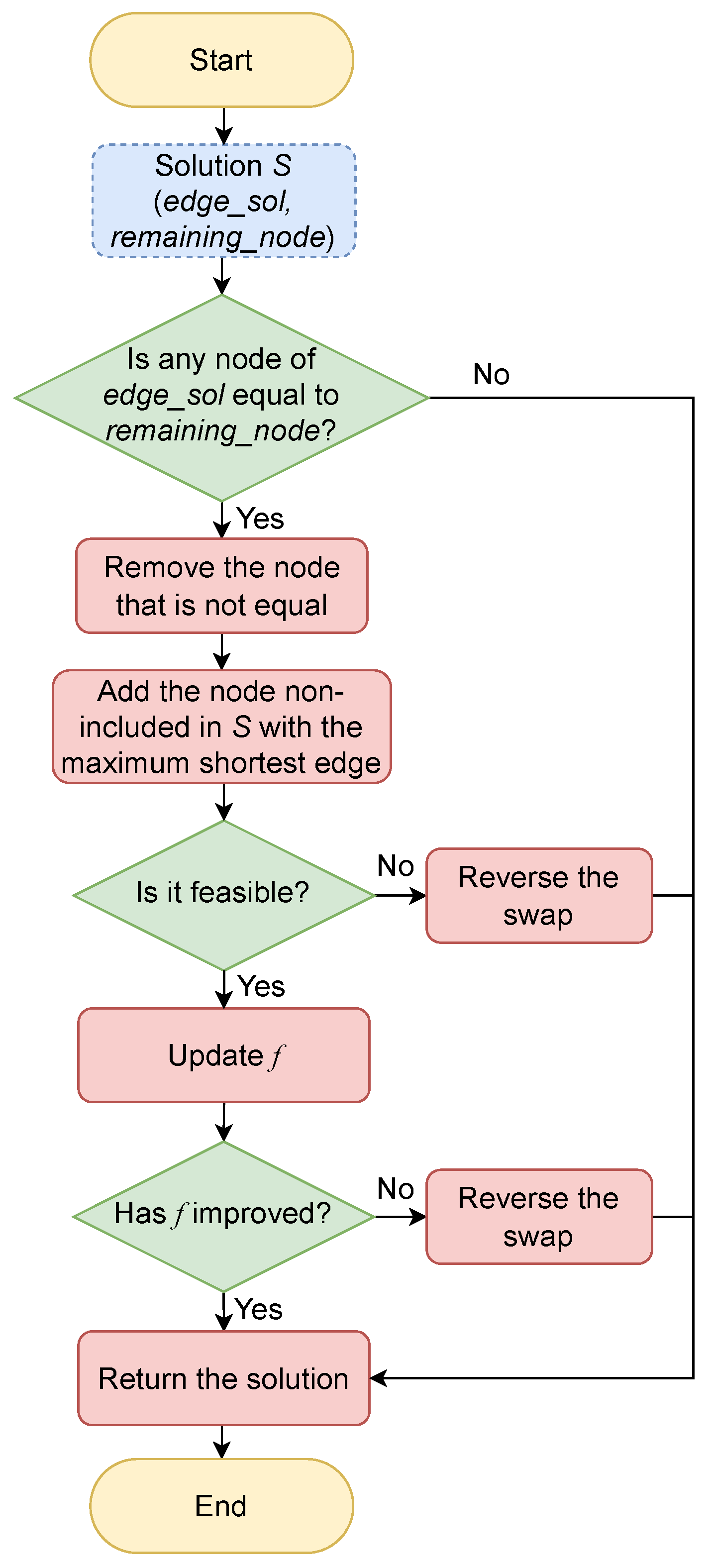
Finally, Algorithm 4 performs a fast last movement (line 12) considering both the shortest edge in the current solution as well as the node that remained in the solution ($remaining\_node$) after assessing the second-to-last edge in the while loop. Figure 2 depicts an overview of the last movement implemented at the end of Algorithm 4. It consists of checking if $remaining\_node$ is the same as any facility in the shortest edge ($edge\_sol$). If it is the same, then we remove the complementary facility in $edge\_sol$, i.e., the facility that is not $remaining\_node$.

Then, we calculate the distances between each node included in the current solution (S) and each facility that is not in S. For each facility non-included in S, we select the edge with the shortest distance, i.e., we have a set of minimum-distance edges. Next, the facility with the longest edge of this set is included in the solution. As a consequence, a new solution is found and, if it is feasible and the value of the objective function improves the original one, the new solution is accepted. This heuristic is fast in terms of the computational time, since it avoids recomputing the entire solution each time a facility is closed.

As in the previous framework, a deterministic version of Algorithm 4 is employed to create an initial solution. Later, this heuristic is embedded into a multi-start iterative process used to improve the initial solution (Algorithm 5). It uses biased-randomization techniques to select the next edge from the list. Again, a geometric probability distribution with parameter $\beta$ ($0<\beta <1$) is employed. This procedure is similar to the one described in Algorithm 2.

Algorithm 4: Destructive heuristic ($edge\_list$)

1: $S\leftarrow Allnodes$ 2: $edge\_list\leftarrow sort(edge\_list$) 3: while$\mathit{feasible}\_\mathit{solution}\left(\mathit{S}\right)$do 4:     Select an element i from $edge\_list$ 5:     $selected\_node\leftarrow SelectNode(edge\_list(i\left)\right)$ 6:     $S\leftarrow S\backslash selected\_node$ 7:     $edge\_list\leftarrow Update(edge\_list,selected\_node)$ 8: end while 9: $S\leftarrow S\cup selected\_node$ 10: $f\leftarrow Update\_f\left(S\right)$ 11: $edge\_list\leftarrow Update(edge\_list,selected\_node)$ 12: $S\leftarrow last\_move(S,edge\_list(i\left)\right)$ 13: returnS

Algorithm 5: Multi-start biased-randomized destructive heuristic ($t_{max},beta,edge\_list$)

1: $S\leftarrow DestructiveHeuristic(edge\_list)$ 2: while$(time\le t_{max})$do 3:     $S_{new}\leftarrow BRDestructivedHeuristic\left(beta\right)$ 4:     $S_{new}^{\prime }\leftarrow LocalSearch\left(S_{new}\right)$ 5:      if $f\left(S_{new}^{\prime }\right)>f\left(S\right)$ then 6:           $S\leftarrow S_{new}^{\prime }$ 7:      end if 8: end while 9: returnS

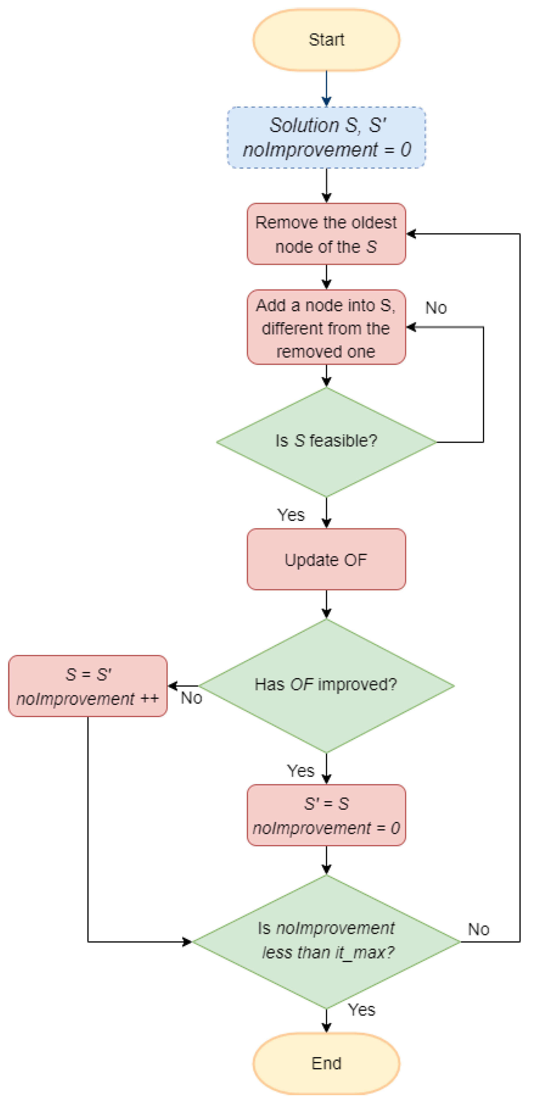
Figure 3 outlines the main characteristics of the local search procedure employed to improve the solution provided by the destructive heuristic. The main idea behind this method is trying to delete the minimum connection between two facilities of the solution. The local search follows a swapping strategy to achieve this goal. The procedure starts by selecting the edge with the shortest distance in the solution S, which defines the best-found objective function. The facility with the smallest capacity in this edge is selected to be swapped with a facility that has not been included in the current solution. After this swapping operation is performed, the solution is recomputed using the constructive heuristic.

The local search procedure follows a first-improved criteria to accept the swap, i.e., each time the solution is enhanced, the local search performs the swap and then selects the new minimum edge to repeat the procedure. Once this method finds a facility that improves the solution for this selected edge, the local search stops, i.e., this procedure does not explore if a different facility yields a higher-quality improvement. The local search finishes when no new improvements are achieved.

5. Numerical Experiments and Results

This section describes the computational experiments that we performed to test the effectiveness and efficiency of the algorithms discussed above.

5.1. Computational Environment

All the algorithms were implemented in Python $3.8$ and executed using a computing instance of Google Cloud Platform (GCP) with an Intel(R) Xeon(R) CPU @ $2.20$ GHz with 4 GB of memory RAM and Ubuntu $18.04$ as the Operating system. We set the maximum execution time to 60 s for the small and medium instances (less than 500 nodes) and 180 s for those with 500 nodes or more.

The proposed algorithms were compared with the BKS reported by Martí et al. [51], who employed both Gurobi and approximate methods as solving approaches. A Geometric probability distribution with parameter $\beta =0.3$ was used for all the performed experiments. This parameter was obtained after a quick test on the set $\{0.1,0.2,\dots ,0.9\}$. Each instance was run 30 times with different random seeds. Three groups of instances proposed by Martí et al. [51] were employed, namely:

• SOM instances, which is a data set with random numbers between 0 and 9 from an integer Uniform distribution. The data set was proposed in Martí et al. [34]. These instances have 50 nodes.
• GKD instances, which is a data set built using Euclidean distances. Node coordinates were generated considering a Uniform distribution between 0 and 10. This data set was proposed in Martí et al. [34]. Two subsets were considered: the first one is called GKD-b and has instances with 50 and 150 nodes; and the second one is called GKD-c and has instances with 500 nodes.
• MDG instances, which is a data set with real numbers randomly selected between 0 and 1000 from a Uniform distribution. This data set was introduced by Duarte and Martí [27]. These instances have 500 nodes.

Since the aforementioned instances were originally proposed to solve the maximum diversity problem—i.e., they did not consider node capacities—we adapted them to include all the CDP characteristics. Hence, Martí et al. [51] assumed that the minimum aggregated capacity b is a percentage m of the sum of all facility capacities, with $m\in \{0.2,0.3\}$ (i.e., $20\%$ or $30\%$ of the total capacity in the network). That is, $b=m·{\sum }_{i\in V}{c}_i$. We divided our experiments into two different sets.

First, to compare the quality of our methods with the BKS, we considered the case where $m=0.2$, which is the level used in Martí et al. [51]. In the second set of experiments, cases where $m\in \{0.4,0.6,0.8\}$ were also tested. These scenarios might appear in some telecommunication networks where many access points, hubs, or antennas have to be deployed [59,60].

5.2. Analysis of Results

Table 1. Comparative results between our algorithms and other approaches.

Instance	Solution Approach							Gaps (%)
	Gurobi (UB) [1]	Martí et al. [51] BKS [2]	GRASP [3]	Constructive Avg [4]	Constructive Best [5]	Destructive Avg [6]	Destructive Best [7]	[1]–[5]	[1]–[7]	[2]–[5]	[2]–[7]	[3]–[5]	[3]–[7]	[5]–[7]
SOM-a_11_n50_m5	4.0	4.0	4.0	4.0	4.0	4.0	4.0	0.0%	0.0%	0.0%	0.0%	0.0%	0.0%	0.0%
SOM-a_12_n50_m5	4.0	4.0	4.0	4.0	4.0	4.0	4.0	0.0%	0.0%	0.0%	0.0%	0.0%	0.0%	0.0%
SOM-a_13_n50_m5	5.0	5.0	5.0	5.0	5.0	5.0	5.0	0.0%	0.0%	0.0%	0.0%	0.0%	0.0%	0.0%
SOM-a_14_n50_m5	4.0	4.0	4.0	4.0	4.0	4.0	4.0	0.0%	0.0%	0.0%	0.0%	0.0%	0.0%	0.0%
SOM-a_15_n50_m5	4.0	4.0	4.0	4.0	4.0	4.0	4.0	0.0%	0.0%	0.0%	0.0%	0.0%	0.0%	0.0%
SOM-a_16_n50_m15	4.0	4.0	4.0	4.0	4.0	4.0	4.0	0.0%	0.0%	0.0%	0.0%	0.0%	0.0%	0.0%
SOM-a_17_n50_m15	4.0	4.0	4.0	4.0	4.0	4.0	4.0	0.0%	0.0%	0.0%	0.0%	0.0%	0.0%	0.0%
SOM-a_18_n50_m15	4.0	4.0	4.0	4.0	4.0	4.0	4.0	0.0%	0.0%	0.0%	0.0%	0.0%	0.0%	0.0%
SOM-a_19_n50_m15	4.0	4.0	4.0	4.0	4.0	4.0	4.0	0.0%	0.0%	0.0%	0.0%	0.0%	0.0%	0.0%
SOM-a_20_n50_m15	4.0	4.0	4.0	4.0	4.0	4.0	4.0	0.0%	0.0%	0.0%	0.0%	0.0%	0.0%	0.0%
GKD-b_11_n50_b02	147.2	147.2	147.2	135.1	147.2	146.6	146.6	0.0%	0.4%	0.0%	0.4%	0.0%	0.4%	0.4%
GKD-b_12_n50_b02	178.1	178.1	178.1	164.9	178.1	178.1	178.1	0.0%	0.0%	0.0%	0.0%	0.0%	0.0%	0.0%
GKD-b_13_n50_b02	96.1	93.6	96.1	83.6	96.1	92.2	92.2	0.0%	4.1%	−2.7%	1.5%	0.0%	4.1%	4.1%
GKD-b_14_n50_b02	84.6	84.6	84.6	73.3	84.6	84.6	84.6	0.0%	0.0%	0.0%	0.0%	0.0%	0.0%	0.0%
GKD-b_15_n50_b02	154.9	154.9	154.9	140.7	154.9	154.9	154.9	0.0%	0.0%	0.0%	0.0%	0.0%	0.0%	0.0%
GKD-b_16_n50_b02	77.7	77.7	77.7	65.8	77.7	77.7	77.7	0.0%	0.0%	0.0%	0.0%	0.0%	0.0%	0.0%
GKD-b_17_n50_b02	41.8	38.2	41.8	33.2	41.8	38.4	38.4	0.0%	8.1%	−9.4%	−0.5%	0.0%	8.1%	8.1%
GKD-b_18_n50_b02	108.5	108.5	108.5	97.6	108.5	105.9	106.6	0.0%	1.8%	0.0%	1.8%	0.0%	1.8%	1.8%
GKD-b_19_n50_b02	119.1	119.1	119.1	106.1	119.1	119.1	119.1	0.0%	0.0%	0.0%	0.0%	0.0%	0.0%	0.0%
GKD-b_20_n50_b02	115.3	115.3	115.3	103.5	115.3	108.7	108.7	0.0%	5.7%	0.0%	5.7%	0.0%	5.7%	5.7%
GKD-b_41_n150_b02	164.2	161.8	161.7	152.7	164.2	157.5	158.7	0.0%	3.3%	−1.5%	1.9%	−1.5%	1.9%	3.3%
GKD-b_42_n150_b02	84.3	84.1	84.0	74.6	84.1	82.9	84.0	0.2%	0.4%	0.0%	0.1%	−0.1%	0.0%	0.1%
GKD-b_43_n150_b02	63.3	62.0	62.0	54.4	62.7	61.5	62.5	0.9%	1.3%	−1.1%	−0.8%	−1.1%	−0.8%	0.3%
GKD-b_44_n150_b02	103.3	101.6	102.2	91.4	102.2	98.1	98.6	1.1%	4.5%	−0.6%	3.0%	0.0%	3.5%	3.5%
GKD-b_45_n150_b02	106.6	105.8	104.9	96.0	106.6	104.4	104.4	0.0%	2.1%	−0.8%	1.3%	−1.6%	0.5%	2.1%
GKD-b_46_n150_b02	124.5	123.8	124.4	113.2	124.5	123.2	123.2	0.0%	1.0%	−0.6%	0.5%	−0.1%	1.0%	1.0%
GKD-b_47_n150_b02	163.4	162.6	163.0	153.2	162.9	162.3	162.5	0.3%	0.6%	−0.2%	0.1%	0.1%	0.3%	0.2%
GKD-b_48_n150_b02	100.2	98.7	98.5	89.3	100.0	98.1	98.1	0.2%	2.1%	−1.3%	0.6%	−1.5%	0.4%	1.9%
GKD-b_49_n150_b02	166.3	165.5	166.3	156.0	166.3	166.0	166.3	0.0%	0.0%	−0.5%	−0.5%	0.0%	0.0%	0.0%
GKD-b_50_n150_b02	111.2	110.3	110.1	100.0	111.2	107.3	108.1	0.0%	2.8%	−0.8%	2.0%	−1.0%	1.8%	2.8%
GKD-c_01_n500_b02	9.4	9.2	9.1	8.3	9.1	9.1	9.1	3.2%	3.2%	1.1%	1.1%	0.0%	0.0%	0.0%
GKD-c_02_n500_b02	9.5	9.3	9.2	8.4	9.4	9.2	9.2	1.1%	3.2%	−1.1%	1.1%	−2.2%	0.0%	2.1%
GKD-c_03_n500_b02	9.4	9.2	9.1	8.3	9.2	8.9	9.0	2.1%	4.3%	0.0%	2.2%	−1.1%	1.1%	2.2%
GKD-c_04_n500_b02	9.3	9.1	9.0	8.2	9.1	9.0	9.1	2.2%	2.2%	0.0%	0.0%	−1.1%	−1.1%	0.0%
GKD-c_05_n500_b02	9.3	9.1	9.0	8.2	9.1	8.9	9.0	2.2%	3.2%	0.0%	1.1%	−1.1%	0.0%	1.1%
GKD-c_06_n500_b02	9.4	9.0	8.9	8.2	9.1	8.9	8.9	3.2%	5.3%	−1.1%	1.1%	−2.2%	0.0%	2.2%
GKD-c_07_n500_b02	9.3	9.1	9.1	8.3	9.1	9.0	9.1	2.2%	2.2%	0.0%	0.0%	0.0%	0.0%	0.0%
GKD-c_08_n500_b02	9.6	9.3	9.3	8.5	9.5	9.2	9.3	1.0%	3.1%	−2.2%	0.0%	−2.2%	0.0%	2.1%
GKD-c_09_n500_b02	9.3	9.1	9.1	8.2	9.0	9.0	9.0	3.2%	3.2%	1.1%	1.1%	1.1%	1.1%	0.0%
GKD-c_10_n500_b02	9.5	9.3	9.1	8.3	9.2	9.1	9.2	3.2%	3.2%	1.1%	1.1%	−1.1%	−1.1%	0.0%
MDG-b_01_n500_b02	125.0	50.6	51.1	37.5	56.9	51.7	54.5	-	-	−12.5%	−7.7%	−11.4%	−6.7%	4.2%
MDG-b_02_n500_b02	125.0	46.0	46.6	33.4	50.9	44.8	50.0	-	-	−10.7%	−8.7%	−9.2%	−7.3%	1.8%
MDG-b_03_n500_b02	125.0	45.8	45.3	33.8	51.4	43.6	45.8	-	-	−12.2%	0.0%	−13.5%	−1.1%	10.9%
MDG-b_04_n500_b02	125.0	47.6	49.6	34.7	53.0	41.5	42.9	-	-	−11.3%	9.9%	−6.9%	13.5%	19.1%
MDG-b_05_n500_b02	125.0	49.1	48.1	34.9	50.7	46.7	49.1	-	-	−3.3%	0.0%	−5.4%	−2.1%	3.2%
MDG-b_06_n500_b02	125.0	46.6	45.4	33.7	49.9	44.6	48.7	-	-	−7.1%	−4.5%	−9.9%	−7.3%	2.4%
MDG-b_07_n500_b02	125.0	47.3	44.9	33.1	47.9	43.4	45.5	-	-	−1.3%	3.8%	−6.7%	−1.3%	5.0%
MDG-b_08_n500_b02	125.0	48.7	45.2	34.0	51.8	48.1	50.1	-	-	−6.4%	−2.9%	−14.6%	−10.8%	3.3%
MDG-b_09_n500_b02	125.0	48.8	47.8	35.9	52.7	46.7	49.9	-	-	−8.0%	−2.3%	−10.3%	−4.4%	5.3%
MDG-b_10_n500_b02	125.0	50.5	47.5	34.9	56.5	47.5	52.7	-	-	−11.9%	−4.4%	−18.9%	−10.9%	6.7%
Average	73.9	58.1	58.1	51.1	59.3	57.1	57.9	0.7%	1.8%	$-2.1$%	0.2%	$-2.5$%	$-0.2$%	2.1%

shows the results obtained with the constructive and destructive heuristics for all benchmark instances when $m=0.2$. Moreover, with the objective to compare the quality of our methods, we also report the obtained results using an implementation of the well-known GRASP metaheuristic, in which the same constructive procedure and local search operators were used, as well as the results reported by Martí et al. [51], employing both Gurobi and approximate methods. The results obtained by the latter are called the BKS.

In the case of the large MDG instances, the values obtained by Gurobi represent only an upper bound attained in 3600 s of computing time. Since we use 10 different seeds, Table 1 shows two columns of results for each heuristic strategy: a column with the average (Avg) result (columns [4] and [6]) when running these 30 seeds, and a column with our best-found solution (columns [5] and [7]). The last six columns in Table 1 show the percentage gaps between some of the tested solution approaches.

Hence, if we denote OBS as the best solution obtained with our biased-randomized algorithm, then the percentage gap between both the BKS and the OBS solutions is computed as $Gap=(BKS-OBS)/BKS$. That is, since the objective function must be maximized, a negative gap means that our algorithm outperforms the current BKS. Finally, the gap regarding the MDG instances when solved by Gurobi is not computed, since these values only represent upper bounds and not the optimal solutions.

As can be seen in Table 1, the OBS obtained by our constructive algorithm usually matches or outperforms the BKS, sometimes by a noticeable percentage gap. For example, while the global average gap between these approaches is $-2.1\%$, we can see that this gap grows up to a $-8.5\%$ for the MDG instances, which are the largest ones. For the smallest instances, the gap is smaller since both the BKS and our constructive algorithm are capable of reaching the optimal value (hence, there is a large number of $0\%$ gaps). For this set of instances, our destructive algorithm does not perform as well as the constructive one but provides an average gap of only $0.2\%$ when compared with the currently published BKS.

Notice that both algorithms also reach the optimal solutions for all SOM instances. Furthermore, the constructive algorithm yields the optimal solution for all the GKD instances with 50 facilities and for a few GKD instances with 150 facilities. Concerning the GRASP metaheuristic, as can be observed, both the constructive and the destructive methods outperform the results provided by the GRASP metaheuristic, obtaining improvements of about $-2.5\%$ and $-0.2\%$, respectively.

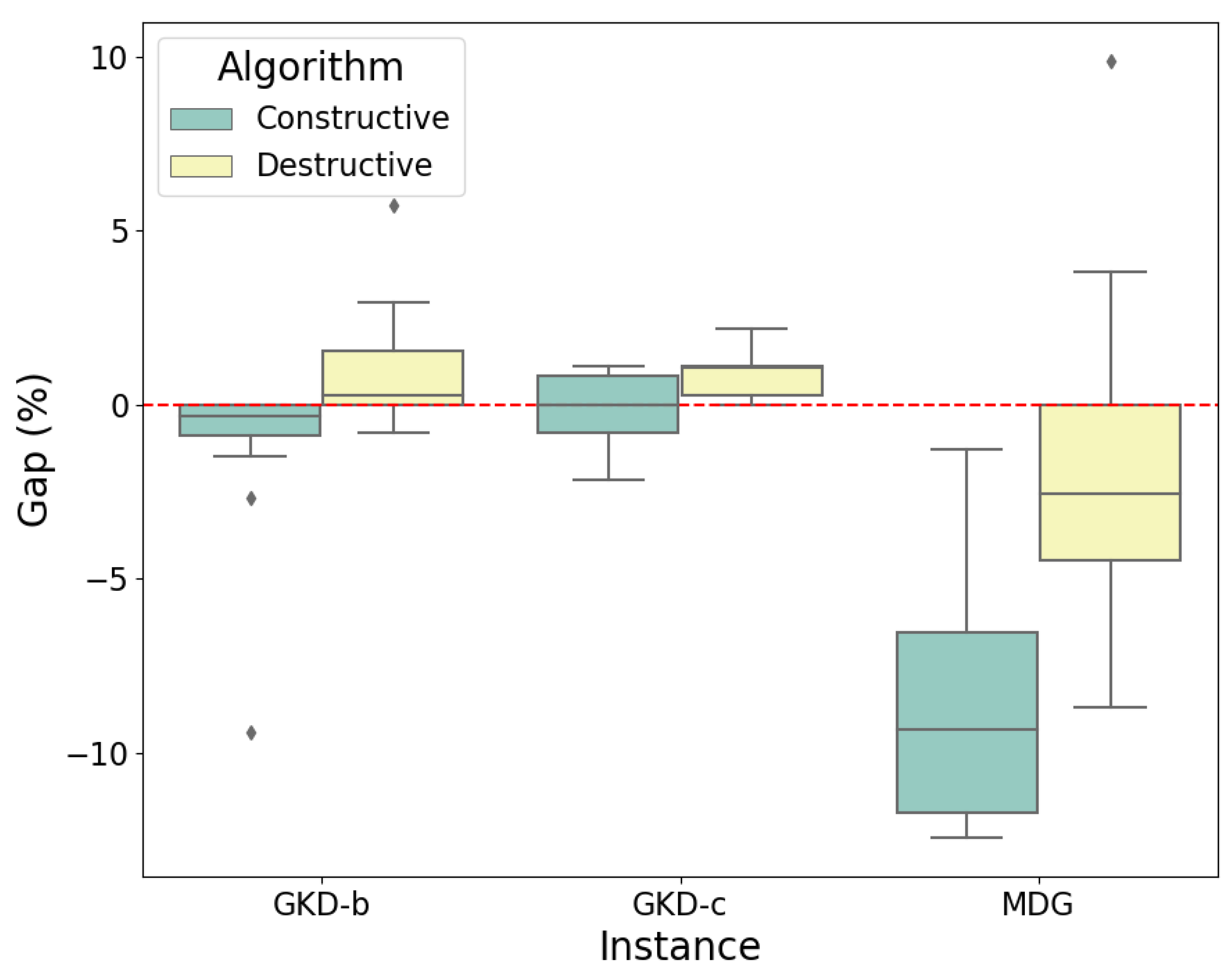
Additionally, we notice that the average gap between the OBS obtained by our constructive algorithm and the optimal solutions is only $0.7\%$. The computed gaps between our approaches and the BKS are depicted in Figure 4. GKD-b, GKD-c, and MDG instances are considered. For each pair of box plots, the one on the left (in green) represents our constructive algorithm, while the one on the right (in yellow) refers to our destructive algorithm. For almost all these instances, the constructive algorithm outperforms the BKS.

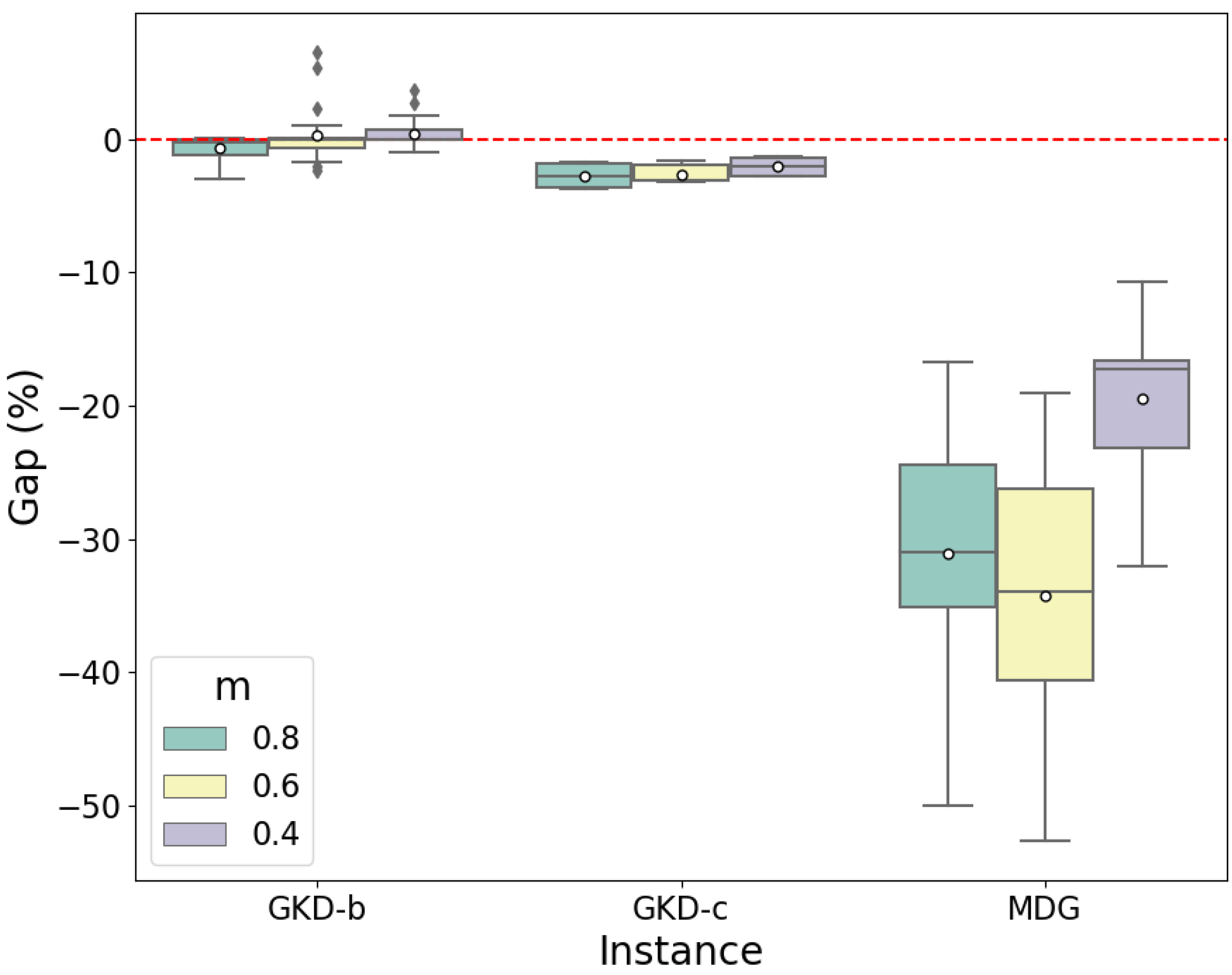
In order to justify why we designed the destructive procedure, additional sets of experiments were conducted. The m parameter was set as $0.8$, $0.6$, and $0.4$.

Table 2. Performance of our algorithm versions for different capacity levels.

Instance	Minimum Aggregate Capacity m
	0.8			0.6			0.4
	Constructive	Destructive	Gap	Constructive	Destructive	Gap	Constructive	Destructive	Gap
GKD-b_11_n50_b02	95.3	95.3	0.0%	107.8	107.8	0.0%	122.4	122.4	0.0%
GKD−b_12_n50_b02	117.7	117.7	0.0%	136.1	136.1	0.0%	148.7	146.1	1.7%
GKD−b_13_n50_b02	43.0	43.0	0.0%	55.1	55.1	0.0%	70.9	70.9	0.0%
GKD−b_14_n50_b02	39.7	39.7	0.0%	47.9	47.9	0.0%	62.5	62.5	0.0%
GKD−b_15_n50_b02	93.0	92.9	0.1%	111.1	109.9	1.1%	129.2	129.2	0.0%
GKD−b_16_n50_b02	22.2	22.2	0.0%	39.0	39.0	0.0%	49.1	49.1	0.0%
GKD−b_17_n50_b02	6.5	6.5	0.0%	13.8	12.9	6.5%	22.5	21.9	2.7%
GKD−b_18_n50_b02	54.8	54.8	0.0%	74.4	72.7	2.3%	88.0	84.8	3.6%
GKD−b_19_n50_b02	64.6	64.6	0.0%	81.0	76.7	5.3%	96.3	96.1	0.2%
GKD−b_20_n50_b02	65.1	65.1	0.0%	77.9	77.9	0.0%	90.1	90.1	0.0%
GKD−b_41_n150_b02	117.4	118.8	−1.2%	129.5	130.3	−0.6%	145.2	143.5	1.2%
GKD−b_42_n150_b02	43.5	43.9	−0.9%	52.8	53.3	−0.9%	64.7	64.9	−0.3%
GKD−b_43_n150_b02	27.6	28.3	−2.5%	37.4	38.0	−1.6%	44.2	44.6	−0.9%
GKD−b_44_n150_b02	56.6	58.3	−3.0%	69.4	69.5	−0.1%	79.5	78.8	0.9%
GKD−b_45_n150_b02	65.9	66.5	−0.9%	75.3	76.6	−1.7%	87.7	88.6	−1.0%
GKD−b_46_n150_b02	76.3	76.8	−0.7%	88.1	89.9	−2.0%	102.2	102.2	0.0%
GKD−b_47_n150_b02	119.1	120.6	−1.3%	131.1	131.6	−0.4%	143.0	143.5	−0.3%
GKD−b_48_n150_b02	57.7	58.6	−1.6%	66.9	68.5	−2.4%	78.2	77.7	0.6%
GKD−b_49_n150_b02	120.6	121.2	−0.5%	133.8	133.3	0.4%	147.1	147.1	0.0%
GKD−b_50_n150_b02	66.1	67.0	−1.4%	77.2	77.3	−0.1%	90.1	89.9	0.2%
GKD−c_01_n500_b02	5.5	5.7	−3.6%	6.4	6.6	−3.1%	7.3	7.5	−2.7%
GKD−c_02_n500_b02	5.7	5.8	−1.8%	6.4	6.6	−3.1%	7.5	7.6	−1.3%
GKD−c_03_n500_b02	5.5	5.7	−3.6%	6.3	6.4	−1.6%	7.3	7.5	−2.7%
GKD−c_04_n500_b02	5.4	5.5	−1.9%	6.3	6.5	−3.2%	7.3	7.5	−2.7%
GKD−c_05_n500_b02	5.5	5.6	−1.8%	6.3	6.5	−3.2%	7.4	7.5	−1.4%
GKD−c_06_n500_b02	5.4	5.6	−3.7%	6.4	6.6	−3.1%	7.3	7.4	−1.4%
GKD−c_07_n500_b02	5.5	5.7	−3.6%	6.4	6.6	−3.1%	7.2	7.4	−2.8%
GKD−c_08_n500_b02	5.4	5.5	−1.9%	6.4	6.6	−3.1%	7.5	7.6	−1.3%
GKD−c_09_n500_b02	5.6	5.7	−1.8%	6.4	6.5	−1.6%	7.3	7.4	−1.4%
GKD−c_10_n500_b02	5.5	5.7	−3.6%	6.4	6.5	−1.6%	7.4	7.6	−2.7%
MDG−b_01_n500_b02	1.4	1.9	−35.7%	4.0	5.0	−25.0%	11.5	14.5	−26.1%
MDG−b_02_n500_b02	1.2	1.6	−33.3%	4.2	5.5	−31.0%	12.2	13.5	−10.7%
MDG−b_03_n500_b02	1.2	1.4	−16.7%	3.7	5.2	−40.5%	10.4	12.3	−18.3%
MDG−b_04_n500_b02	1.2	1.6	−33.3%	3.5	5.1	−45.7%	9.6	11.0	−14.6%
MDG−b_05_n500_b02	1.2	1.7	−41.7%	3.7	4.8	−29.7%	10.5	13.1	−24.8%
MDG−b_06_n500_b02	1.3	1.6	−23.1%	3.7	5.2	−40.5%	11.2	13.1	−17.0%
MDG−b_07_n500_b02	1.5	1.8	−20.0%	4.2	5.0	−19.0%	10.6	14.0	−32.1%
MDG−b_08_n500_b02	1.4	1.8	−28.6%	4.7	5.7	−21.3%	13.8	16.2	−17.4%
MDG−b_09_n500_b02	1.4	1.8	−28.6%	3.8	5.8	−52.6%	12.7	14.8	−16.5%
MDG−b_10_n500_b02	1.2	1.8	−50.0%	3.8	5.2	−36.8%	11.4	13.4	−17.1%
Average	35.5	35.9	−8.8%	42.7	43.1	−9.1%	51.2	51.6	−5.2%

compares the performance of the constructive and destructive versions of the algorithm under these conditions. SOM instances are not included in this table because the optimal solutions are always $0.0$ when $m=0.8$ and $m=0.6$, and $1.0$ when $m=0.4$. That is, the best solution under these conditions is a trivial one given the characteristics of the SOM instances—e.g., the input distance between some pairs of potential facilities is $0.0$.

In Table 2, the gap is calculated as Gap = (constructive − destructive)/constructive, i.e., a negative gap means that the destructive version reaches a higher quality solution, whereas a positive gap means that the constructive procedure is better. Unlike the results in Table 1, where the aggregate capacity was set in $20\%$, Table 2 shows a general better performance of the destructive procedure. This is mainly because this set of instances requires a high percentage of open facilities to reach optimality.

The highest average differences are achieved when $m=0.8$ ($-8.8\%$) and $m=0.6$ ($-9.1\%$). When $m=0.4$, the gap decreases to $-5.2\%$, and, as previously shown, the average difference is $2.1\%$ when $m=0.2$. A general decreasing trend in the solution quality is identified when increasing m. For instance, the destructive procedure yields an average solution of $71.1$ when $m=0.2$ (Table 1), whereas this solution is $35.9$ when $m=0.8$. Notice that this situation is explained by the fact that a higher capacity percentage requires to open a higher number of facilities.

As a result, the distances between open facilities are smaller. Furthermore, we highlight the high gap difference for the MDG instances. For example, when $m=0.6$, the average difference computed only for these instances is $-34.2\%$, with a maximum gap of $-52.6\%$ for a single instance. These results demonstrate the necessity of a destructive procedure such as the one designed in this article. Finally, Figure 5 shows a percentage comparison between the constructive and destructive versions of the algorithm for different levels of m and considering the GKD-b, GKD-c, and MDG instances.

These box plots highlight the large differences between the obtained results. For example, the results for the MDG instances show that the destructive version clearly outperforms the constructive version, regardless of the m value. In contrast, when considering the GKD instances, the differences are not so noticeable.

6. Conclusions and Future Work

In this work, we proposed a constructive–destructive biased-randomized algorithm to solve the CDP. A multi-start approach, including a local search procedure, allowed us to diversify and intensify the search. The first algorithm version used a constructive approach: starting from a scenario with no selected elements (facilities), the solution was constructed by iteratively adding promising elements, one at a time, until the required servicing capacity was reached. On the contrary, the destructive version began with all elements selected.

Then, the solution was constructed by removing non-promising elements, one at a time, while the required servicing capacity was still satisfied. Since most existing benchmark instances are designed to solve the MDP, which does not consider facility capacities, the minimum required capacity must be included in the instances. Different values for this parameter were considered, which was set as a percentage of the total potential capacity in the network. In particular, we conducted experiments where this parameter, m, was set as $0.2$, $0.4$, $0.6$, and $0.8$. The case where $m=0.2$ allowed us to perform comparisons between our two versions of the algorithm and the state-of-the-art approaches.

In this case, the obtained results show the potential of our constructive version, which was able to outperform the recently published best-known solutions for large instances with 500 elements. Additionally, our destructive version of the algorithm also yielded competitive results for these instances.

In a second set of experiments, the approaches were compared for higher values of m. In this case, the destructive version of the algorithm outperformed the constructive one, especially when $m=0.6$ and $m=0.8$. These results show that, as the number of elements to select increased, removing elements from an ‘all-selected’ scenario was a more efficient strategy than starting from an ‘none-selected’ scenario. On the contrary, when the number of needed elements was small, the constructive strategy tended to perform better. Notice that our approach allowed us to perform a fast heuristic test on each instance to determine which strategy (constructive or destructive) would perform better for that specific instance and then to use that strategy in the full metaheuristic algorithm.

Some future research lines that can extend this work are described next: (i) to consider a variant of the problem in which there is a cost associated with selecting each element (e.g., the cost of opening a given facility, which should be related to the capacity of each facility); and (ii) to consider realistic scenarios where the input parameters—such as the demands or capacities—are stochastic. In this case, our proposed algorithms can be extended into a simheuristic by including Monte Carlo simulation.

References

- Govindan, K.; Fattahi, M.; Keyvanshokooh, E. Supply chain network design under uncertainty: A comprehensive review and future research directions. Eur. J. Oper. Res. 2017, 263, 108–141. [Google Scholar] [CrossRef]
- Eskandarpour, M.; Dejax, P.; Miemczyk, J.; Péton, O. Sustainable supply chain network design: An optimization-oriented review. Omega 2015, 54, 11–32. [Google Scholar] [CrossRef]
- Correia, I.; Saldanha-da Gama, F. Facility location under uncertainty. In Location Science; Springer: Berlin/Heidelberg, Germany, 2015; pp. 185–213. [Google Scholar]
- Fernández, E.; Landete, M. Fixed-charge facility location problems. In Location Science; Springer: Berlin/Heidelberg, Germany, 2015; pp. 47–77. [Google Scholar]
- Dönmez, Z.; Kara, B.Y.; Karsu, Ö.; Saldanha-da Gama, F. Humanitarian facility location under uncertainty: Critical review and future prospects. Omega 2021, 102, 102393. [Google Scholar] [CrossRef]
- Ortiz-Astorquiza, C.; Contreras, I.; Laporte, G. Multi-level facility location problems. Eur. J. Oper. Res. 2018, 267, 791–805. [Google Scholar] [CrossRef] [Green Version]
- Boonmee, C.; Arimura, M.; Asada, T. Facility location optimization model for emergency humanitarian logistics. Int. J. Disaster Risk Reduct. 2017, 24, 485–498. [Google Scholar] [CrossRef]
- Ahmadi-Javid, A.; Seyedi, P.; Syam, S.S. A survey of healthcare facility location. Comput. Oper. Res. 2017, 79, 223–263. [Google Scholar] [CrossRef]
- Melo, M.T.; Nickel, S.; Saldanha-Da-Gama, F. Facility location and supply chain management—A review. Eur. J. Oper. Res. 2009, 196, 401–412. [Google Scholar] [CrossRef]
- Pagès-Bernaus, A.; Ramalhinho, H.; Juan, A.A.; Calvet, L. Designing e-commerce supply chains: A stochastic facility–location approach. Int. Trans. Oper. Res. 2019, 26, 507–528. [Google Scholar] [CrossRef]
- De Armas, J.; Juan, A.A.; Marquès, J.M.; Pedroso, J.P. Solving the deterministic and stochastic uncapacitated facility location problem: From a heuristic to a simheuristic. J. Oper. Res. Soc. 2017, 68, 1161–1176. [Google Scholar] [CrossRef]
- Fernandez, S.; Juan, A.A.; de Armas, J.; Silva, D.; Riera, D. Metaheuristics in telecommunication systems: Network design, routing, and allocation problems. IEEE Syst. J. 2018, 12, 3948–3957. [Google Scholar] [CrossRef]
- Martí, R.; Martínez-Gavara, A.; Pérez-Peló, S.; Sánchez-Oro, J. A review on discrete diversity and dispersion maximization from an OR perspective. Eur. J. Oper. Res. 2021, 299, 795–813. [Google Scholar] [CrossRef]
- Sandoya, F.; Martínez-Gavara, A.; Aceves, R.; Duarte, A.; Martí, R. Diversity and equity models. In Handbook of Heuristics; Springer: Berlin/Heidelberg, Germany, 2018; Volume 2, pp. 979–998. [Google Scholar]
- Glover, F.; Kuo, C.C.; Dhir, K.S. Heuristic algorithms for the maximum diversity problem. J. Inf. Optim. Sci. 1998, 19, 109–132. [Google Scholar] [CrossRef]
- Resende, M.G.; Martí, R.; Gallego, M.; Duarte, A. GRASP and path relinking for the max–min diversity problem. Comput. Oper. Res. 2010, 37, 498–508. [Google Scholar] [CrossRef]
- Correia, I.; Melo, T.; Saldanha-da Gama, F. Comparing classical performance measures for a multi-period, two-echelon supply chain network design problem with sizing decisions. Comput. Ind. Eng. 2013, 64, 366–380. [Google Scholar] [CrossRef] [Green Version]
- Tordecilla, R.D.; Copado-Méndez, P.J.; Panadero, J.; Quintero-Araujo, C.L.; Montoya-Torres, J.R.; Juan, A.A. Combining heuristics with simulation and fuzzy logic to solve a flexible-size location routing problem under uncertainty. Algorithms 2021, 14, 45. [Google Scholar] [CrossRef]
- Peiró, J.; Jiménez, I.; Laguardia, J.; Martí, R. Heuristics for the capacitated dispersion problem. Int. Trans. Oper. Res. 2021, 28, 119–141. [Google Scholar] [CrossRef]
- Erkut, E.; Neuman, S. Analytical models for locating undesirable facilities. Eur. J. Oper. Res. 1989, 40, 275–291. [Google Scholar] [CrossRef]
- Martínez-Gavara, A.; Corberán, T.; Martí, R. GRASP and Tabu Search for the Generalized Dispersion Problem. Expert Syst. Appl. 2021, 173, 114703. [Google Scholar] [CrossRef]
- Daskin, M.S. Network and Discrete Location: Models, Algorithms, and Applications; John Wiley & Sons: Hoboken, NJ, USA, 2011. [Google Scholar]
- Lozano-Osorio, I.; Martínez-Gavara, A.; Martí, R.; Duarte, A. Max–min dispersion with capacity and cost for a practical location problem. Expert Syst. Appl. 2022, 200, 116899. [Google Scholar] [CrossRef]
- Rosenkrantz, D.J.; Tayi, G.K.; Ravi, S.S. Facility Dispersion Problems under Capacity and Cost Constraints. J. Comb. Optim. 2000, 4, 7–33. [Google Scholar] [CrossRef]
- Belloso, J.; Juan, A.A.; Faulin, J. An iterative biased-randomized heuristic for the fleet size and mix vehicle-routing problem with backhauls. Int. Trans. Oper. Res. 2019, 26, 289–301. [Google Scholar] [CrossRef] [Green Version]
- Ferone, D.; Hatami, S.; González-Neira, E.M.; Juan, A.A.; Festa, P. A biased-randomized iterated local search for the distributed assembly permutation flow-shop problem. Int. Trans. Oper. Res. 2020, 27, 1368–1391. [Google Scholar] [CrossRef]
- Duarte, A.; Martí, R. Tabu search and GRASP for the maximum diversity problem. Eur. J. Oper. Res. 2007, 178, 71–84. [Google Scholar] [CrossRef]
- Chandrasekaran, R.; Daughety, A. Location on Tree Networks: P-Centre and n-Dispersion Problems. Math. Oper. Res. 1981, 6, 50–57. [Google Scholar] [CrossRef] [Green Version]
- Kuo, C.C.; Glover, F.; Dhir, K.S. Analyzing and Modeling the Maximum Diversity Problem by Zero-One Programming. Decis. Sci. 1993, 24, 1171–1185. [Google Scholar] [CrossRef]
- Ghosh, J.B. Computational aspects of the maximum diversity problem. Oper. Res. Lett. 1996, 19, 175–181. [Google Scholar] [CrossRef] [Green Version]
- Prokopyev, O.A.; Kong, N.; Martinez-Torres, D.L. The equitable dispersion problem. Eur. J. Oper. Res. 2009, 197, 59–67. [Google Scholar] [CrossRef]
- Parreño, F.; Álvarez-Valdés, R.; Martí, R. Measuring diversity. A review and an empirical analysis. Eur. J. Oper. Res. 2021, 289, 515–532. [Google Scholar] [CrossRef]
- Martí, R.; Gallego, M.; Duarte, A.; Pardo, E.G. Heuristics and metaheuristics for the maximum diversity problem. J. Heuristics 2013, 19, 591–615. [Google Scholar] [CrossRef]
- Martí, R.; Gallego, M.; Duarte, A. A branch and bound algorithm for the maximum diversity problem. Eur. J. Oper. Res. 2010, 200, 36–44. [Google Scholar] [CrossRef]
- Lozano, M.; Molina, D.; García-Martínez, C. Iterated greedy for the maximum diversity problem. Eur. J. Oper. Res. 2011, 214, 31–38. [Google Scholar] [CrossRef]
- Zhou, Y.; Hao, J.K.; Duval, B. Opposition-based memetic search for the maximum diversity problem. IEEE Trans. Evol. Comput. 2017, 21, 731–745. [Google Scholar] [CrossRef] [Green Version]
- Aringhieri, R.; Cordone, R. Comparing local search metaheuristics for the maximum diversity problem. J. Oper. Res. Soc. 2011, 62, 266–280. [Google Scholar] [CrossRef]
- Mladenović, N.; Todosijević, R.; Urošević, D. Less is more: Basic variable neighborhood search for minimum differential dispersion problem. Inf. Sci. 2016, 326, 160–171. [Google Scholar] [CrossRef]
- Duarte, A.; Sánchez-Oro, J.; Resende, M.G.; Glover, F.; Martí, R. Greedy randomized adaptive search procedure with exterior path relinking for differential dispersion minimization. Inf. Sci. 2015, 296, 46–60. [Google Scholar] [CrossRef]
- Wang, Y.; Wu, Q.; Glover, F. Effective metaheuristic algorithms for the minimum differential dispersion problem. Eur. J. Oper. Res. 2017, 258, 829–843. [Google Scholar] [CrossRef]
- Zhou, Y.; Hao, J.K. An iterated local search algorithm for the minimum differential dispersion problem. Knowl.-Based Syst. 2017, 125, 26–38. [Google Scholar] [CrossRef] [Green Version]
- Lai, X.; Hao, J.K.; Glover, F.; Yue, D. Intensification-driven tabu search for the minimum differential dispersion problem. Knowl.-Based Syst. 2019, 167, 68–86. [Google Scholar] [CrossRef]
- Martí, R.; Sandoya, F. GRASP and path relinking for the equitable dispersion problem. Comput. Oper. Res. 2013, 40, 3091–3099. [Google Scholar] [CrossRef]
- Lai, X.; Hao, J.K. A tabu search based memetic algorithm for the max-mean dispersion problem. Comput. Oper. Res. 2016, 72, 118–127. [Google Scholar] [CrossRef] [Green Version]
- Carrasco, R.; Pham, A.; Gallego, M.; Gortázar, F.; Martí, R.; Duarte, A. Tabu search for the Max-Mean Dispersion Problem. Knowl.-Based Syst. 2015, 85, 256–264. [Google Scholar] [CrossRef]
- Brimberg, J.; Mladenović, N.; Todosijević, R.; Urošević, D. Less is more: Solving the Max-Mean diversity problem with variable neighborhood search. Inf. Sci. 2017, 382–383, 179–200. [Google Scholar] [CrossRef]
- Lai, X.; Yue, D.; Hao, J.K.; Glover, F. Solution-based tabu search for the maximum min-sum dispersion problem. Inf. Sci. 2018, 441, 79–94. [Google Scholar] [CrossRef]
- Amirgaliyeva, Z.; Mladenović, N.; Todosijević, R.; Urošević, D. Solving the maximum min-sum dispersion by alternating formulations of two different problems. Eur. J. Oper. Res. 2017, 260, 444–459. [Google Scholar] [CrossRef]
- Martínez-Gavara, A.; Campos, V.; Laguna, M.; Martí, R. Heuristic solution approaches for the maximum minsum dispersion problem. J. Glob. Optim. 2017, 67, 671–686. [Google Scholar] [CrossRef]
- Lai, X.; Fu, Z.H. A tabu search approach with dynamical neighborhood size for solving the maximum min-sum dispersion problem. IEEE Access 2019, 7, 181357–181368. [Google Scholar] [CrossRef]
- Martí, R.; Martínez-Gavara, A.; Sánchez-Oro, J. The capacitated dispersion problem: An optimization model and a memetic algorithm. Memetic Comput. 2021, 13, 131–146. [Google Scholar] [CrossRef]
- Sayyady, F.; Fathi, Y. An integer programming approach for solving the p-dispersion problem. Eur. J. Oper. Res. 2016, 253, 216–225. [Google Scholar] [CrossRef]
- Juan, A.A.; Corlu, C.G.; Tordecilla, R.D.; de la Torre, R.; Ferrer, A. On the use of biased-randomized algorithms for solving non-smooth optimization problems. Algorithms 2020, 13, 8. [Google Scholar] [CrossRef] [Green Version]
- Grasas, A.; Juan, A.A.; Faulin, J.; De Armas, J.; Ramalhinho, H. Biased randomization of heuristics using skewed probability distributions: A survey and some applications. Comput. Ind. Eng. 2017, 110, 216–228. [Google Scholar] [CrossRef]
- Juan, A.A.; Faulin, J.; Ferrer, A.; Lourenço, H.R.; Barrios, B. MIRHA: Multi-start biased randomization of heuristics with adaptive local search for solving non-smooth routing problems. TOP 2013, 21, 109–132. [Google Scholar] [CrossRef]
- Ferrer, A.; Guimarans, D.; Ramalhinho, H.; Juan, A.A. A BRILS metaheuristic for non-smooth flow-shop problems with failure-risk costs. Expert Syst. Appl. 2016, 44, 177–186. [Google Scholar] [CrossRef] [Green Version]
- Dominguez, O.; Juan, A.A.; De La Nuez, I.; Ouelhadj, D. An ILS-biased randomization algorithm for the two-dimensional loading HFVRP with sequential loading and items rotation. J. Oper. Res. Soc. 2016, 67, 37–53. [Google Scholar] [CrossRef] [Green Version]
- Estrada-Moreno, A.; Savelsbergh, M.; Juan, A.A.; Panadero, J. Biased-randomized iterated local search for a multiperiod vehicle routing problem with price discounts for delivery flexibility. Int. Trans. Oper. Res. 2019, 26, 1293–1314. [Google Scholar] [CrossRef]
- Alvarez, S.; Ferone, D.; Juan, A.A.; Silva, D.; de Armas, J. A 2-stage biased-randomized iterated local search for the uncapacitated single allocation p-hub median problem. Trans. Emerg. Telecommun. Technol. 2018, 29, e3418. [Google Scholar] [CrossRef]
- Alvarez, S.; Ferone, D.; Juan, A.; Tarchi, D. A simheuristic algorithm for video streaming flows optimisation with QoS threshold modelled as a stochastic single-allocation p-hub median problem. J. Simul. 2021. [Google Scholar] [CrossRef]
Figure 1.
Simple example of a CDP solution.
Figure 2.
Last move of the destructive heuristic.
Figure 3.
Local search (LS).
Figure 4.
Gaps between the BKS and our algorithms.
Figure 5.
Gaps between our algorithms for different minimum capacities.