A (2+1)-Dimensional Fractional-Order Epidemic Model with Pulse Jumps for Omicron COVID-19 Transmission and Its Numerical Simulation

Abstract

In this paper, we would like to propose a (2+1)-dimensional fractional-order epidemic model with pulse jumps to describe the spread of the Omicron variant of COVID-19. The problem of identifying the involved parameters in the proposed model is reduced to a minimization problem of a quadratic objective function, based on the reported data. Moreover, we perform numerical simulation to study the effect of the parameters in diverse fractional-order cases. The number of undiscovered cases can be calculated precisely to assess the severity of the outbreak. The results by numerical simulation show that the degree of accuracy is higher than the classical epidemic models. The regular testing protocol is very important to find the undiscovered cases in the beginning of the outbreak.

1. Introduction

Many mathematical models are proposed to describe the spread of infectious diseases, and the following classical SEIR model is commonly used for disease modeling, which is shown in the following form [1].

$$\begin{array}{c}\hfill \left\{\begin{array}{c}{S}^{\prime }=-\alpha S-\beta S+\gamma R,\hfill \\ I^{\prime }=\alpha S+\eta E-\omega I,\hfill \\ E^{\prime }=\beta S-\eta E,\hfill \\ R^{\prime }=\omega I-\gamma R.\hfill \end{array}\right.\end{array}$$

(1)

In this model, the symbol ′ represents the derivative with respect to the time variable t. We denote $S\equiv S\left(t\right)$, $I\equiv I\left(t\right)$, $E\equiv E\left(t\right)$, and $R\equiv R\left(t\right)$ by the number of each group at time t. In the above model (1), all the population is divided into four groups: susceptible individuals in the free environment (S), undiagnosed and non-isolated infectious individuals (I), free exposed individuals (E), and recovered individuals (R). Considering that the COVID-19 has more complex characteristics than common epidemics, scientists have proposed various generalized SEIR models for describing the spread of COVID-19 (see, e.g., [2,3,4,5,6]). For example, stability analysis and numerical simulation of a generalized SEIR model on the spread of COVID-19 were conducted [2,3]. For another example, the SEIRD model is proposed, in which the total population is divided into five groups, consisting of susceptible, exposed, infected, recovered, and dead. A machine learning algorithm has also been introduced to solve the inverse problem of the SEIRD model [4].

Recently, the highly infectious Omicron variant of COVID-19 has upended many aspects of our lives. However, when the reported data are applied in the above integer-order model to predict the spread of the Omicron variant, the model does not meet the requirements of accuracy, and so, it is invalid. Therefore, the use of a fractional-order model to simulate the Omicron variant of COVID-19 has attracted more and more attention of researchers [7,8,9,10,11,12,13]. Though the degree of accuracy of fraction-order epidemic models is higher than integer-order epidemic models, the birth pulses and pulse treatments dealing with the analysis for the Omicron variant of COVID-19 are not extensive, but these technologies are wildly used in epidemic models [14,15,16,17,18,19,20,21,22]. Therefore, we would like to propose a new (2+1)-dimensional fractional-order epidemic model with pulse jumps to describe the spread of the Omicron variant of COVID-19 in several districts in this paper.

The rest of the paper is organized as follows. In the next section, a new (2+1)-dimensional fractional-order epidemic model with pulse jumps is proposed. In Section 3, the inverse problem is proposed to determine the characteristic parameters in the proposed model, which are used to analyze the spread of the Omicron variant of COVID-19. Numerical simulations are performed in Section 4. At the end of the paper, a few concluding remarks are presented in Section 5.

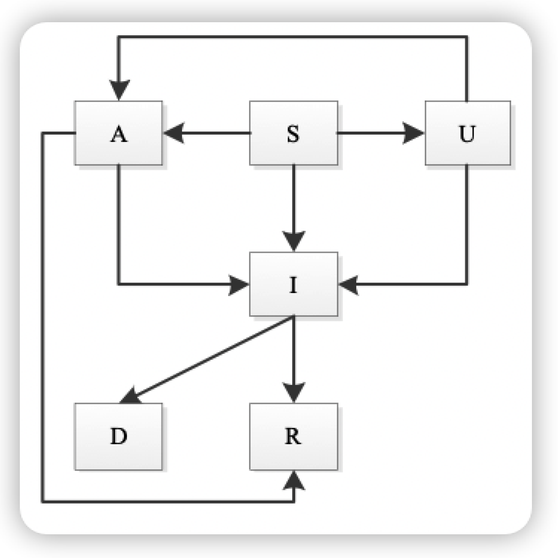
2. Fractional-Order Model with Pulse Jumps

In our model, the total population is divided into six distinct epidemiological subclasses of individuals, which are susceptible (S), asymptomatic (A), infectious (I), recovered (R), dead (D), and unexposed (U). The relationship among the subclasses in the same location is shown in Figure 1.

There are several areas to be considered in this paper, which are denoted as $i=1,2,\dots$. We denote $S\equiv S(i,t)$, $A\equiv A(i,t)$, $I\equiv I(i,t)$, $R\equiv R(i,t)$, $D\equiv D(i,t)$, $U\equiv U(i,t)$ as the number of each group at time t and area i with the location of $(x_i,y_i)$. Suspected cases might be infected to become infectious cases, and the number of infected individuals entering the I class is ${\gamma }_{3}S(I+U+A)$. Suspected cases might be infected to become asymptomatic cases, and the number of infected individuals entering the A class is ${\gamma }_{4}S(I+U+A)$. Suspected cases might be misdiagnosed, and the number of misdiagnosed individuals entering the U class is ${\gamma }_{5}S(I+U+A)$. Therefore, the transfer relationships between class S and the other classes can be expressed as follows:

$${}^c{D}_t^{\alpha }S={\gamma }_1(\frac{{\partial }^{2}S}{\partial x^2}+\frac{{\partial }^{2}S}{\partial y^2})-({\gamma }_3+{\gamma }_4+{\gamma }_5)S(I+U+A).$$

(2)

Here, we adopted the Caputo definition of a fractional-order derivative operator, which is defined in the following form with $m\in {\mathrm{N}}^{+}$:

$${}^c{D}_t^{\alpha }S\left(t\right)=\frac{1}{\mathsf{\Gamma }(m-\alpha )}{\int }_0^t{(t-\tau )}^{-\alpha -1+m}\frac{d^m}{d{\tau }^m}S\left(\tau \right)d\tau ,m-1<\alpha <m.$$

(3)

In many senses, the order of a fractional-order derivative is always less than 1. It is important to point out that there are many definitions of fractional-order derivative operators such as the Grünwald–Letnikov, the Riemann–Liouville, and the Caputo definitions [23,24,25].

When the asymptomatic cases and undiscovered cases are confirmed, the number of infected cases will increase at a rate of ${\gamma }_6$ and ${\gamma }_7$, respectively. The infectious individuals might recover at a rate of ${\gamma }_8$. We denote by ${\gamma }_9$ the death rate of the Omicron variant of COVID-19. Therefore, the transfer relationships between class I and the other classes can be expressed as follows:

$${}^c{D}_t^{\alpha }I={\gamma }_{3}S(I+U+A)+{\gamma }_{6}A+{\gamma }_{7}U-{\gamma }_{8}I-{\gamma }_{9}I+\sum _{i=1}^m{h}_i^{\left(1\right)}\delta (t-t_i).$$

(4)

We denote by ${\gamma }_{10}$ and ${\gamma }_{11}$ the recovery rate of the untreated asymptomatic cases and the rate of the undiscovered cases transferring into class A, respectively. A large number of asymptomatic cases might be reported. We use the following pulse function and delta function to describe such a situation.

$$\begin{array}{c}{\delta }_{\eta }(x-x_0)=\left\{\begin{array}{c}\frac{1}{2\eta },x_0-\eta <x<x_0+\eta ,\hfill \\ 0,\mathrm{otherwise},\hfill \end{array}\right.\hfill \\ \delta (x-x_0)=\underset{\eta \to 0}{\lim }{\delta }_{\eta }(x-x_0).\hfill \end{array}$$

(5)

We also denote by $h_i$ the number of pulse cases at time $t_i$. Therefore, the transfer relationships between class A and the other classes can be expressed as follows:

$${}^c{D}_t^{\alpha }A={\gamma }_{4}S(I+U+A)-{\gamma }_{6}A-{\gamma }_{10}A+{\gamma }_{11}U+\sum _{i=1}^m{h}_i^{\left(2\right)}\delta (t-t_i).$$

(6)

Based on the analysis above, the transfer relationships between class U, class R, class D, and the other classes can be expressed as follows:

$$\begin{array}{c}{}^c{D}_t^{\alpha }U={\gamma }_{5}S(I+U+A)-{\gamma }_{11}U-{\gamma }_{7}U+{\gamma }_2(\frac{{\partial }^{2}U}{\partial x^2}+\frac{{\partial }^{2}U}{\partial y^2}),\hfill \\ {}^c{D}_t^{\alpha }R={\gamma }_{8}I+{\gamma }_{10}A,\hfill \\ {}^c{D}_t^{\alpha }D={\gamma }_{9}I.\hfill \end{array}$$

Thus, we have structured a new model for Omicron COVID-19 infection within the framework of the Caputo fractional-order derivative as follows:

$$\left\{\begin{array}{c}{}^c{D}_t^{\alpha }S={\gamma }_1(\frac{{\partial }^{2}S}{\partial x^2}+\frac{{\partial }^{2}S}{\partial y^2})-({\gamma }_3+{\gamma }_4+{\gamma }_5)S(I+U+A),\hfill \\ {}^c{D}_t^{\alpha }I={\gamma }_{3}S(I+U+A)+{\gamma }_{6}A+{\gamma }_{7}U-{\gamma }_{8}I-{\gamma }_{9}I+\sum _{i=1}^m{h}_i^{\left(1\right)}\delta (t-t_i),\hfill \\ {}^c{D}_t^{\alpha }A={\gamma }_{4}S(I+U+A)-{\gamma }_{6}A-{\gamma }_{10}A+{\gamma }_{11}U+\sum _{i=1}^m{h}_i^{\left(2\right)}\delta (t-t_i),\hfill \\ {}^c{D}_t^{\alpha }U={\gamma }_{5}S(I+U+A)-{\gamma }_{11}U-{\gamma }_{7}U+{\gamma }_2(\frac{{\partial }^{2}U}{\partial x^2}+\frac{{\partial }^{2}U}{\partial y^2}),\hfill \\ {}^c{D}_t^{\alpha }R={\gamma }_{8}I+{\gamma }_{10}A,\hfill \\ {}^c{D}_t^{\alpha }D={\gamma }_{9}I.\hfill \end{array}\right.$$

(7)

The definitions of the parameters are listed in

Table 1. Definition of the parameters.

Symbols	Description
${\gamma }_1$	Transmission rate from S group in other considered locations
${\gamma }_2$	Transmission rate from U group in other considered locations
${\gamma }_3$	Transmission rate from S to I group
${\gamma }_4$	Transmission rate from S to A group
${\gamma }_5$	Transmission rate from S to U group
${\gamma }_6$	Transmission rate from A to I group
${\gamma }_7$	Transmission rate from U to I group
${\gamma }_8$	Recovery rate of I group
${\gamma }_9$	Omicron COVID-19 death rate
${\gamma }_{10}$	Recovery rate of A group
${\gamma }_{11}$	Transmission rate from U to A group

. The initial data are denoted by $I(i,0)$, $A(i,0)$, $R(i,0)$, and $D(i,0)$. ${\gamma }_1$ is the transmission rate from the S group in location $(x_j,y_j)$ to the S group in location $(x_i,y_i)$, $i\ne j$. ${\gamma }_2$ is the transmission rate from the U group in location $(x_j,y_j)$ to the U group in location $(x_i,y_i)$, $i\ne j$. We assume ${\gamma }_1$ and ${\gamma }_2$ are constants in this paper.

3. Inverse Problem

In this section, the discrete-time model is built and the least-squares algorithm is used to solve the inverse problem and estimate the unknown parameters in the model. The reported active cases, recovered cases, death cases, and asymptomatic cases at time $t=n\tau ,n\in N^{*}$ are denoted by $I\left[n\right]$, $R\left[n\right]$, $D\left[n\right]$, and $A\left[n\right]$. Denote $\tau$ as the constant time step, $\tau =1$ usually.

The discrete-time fractional-order Caputo operator ${\mathsf{\Delta }}^{\alpha }$ with numerical approximation is defined in the following form [26].

$$\begin{array}{cc}\hfill {\mathsf{\Delta }}^{\alpha }X\left[n\right]& =\frac{{\tau }^{-\alpha }}{\mathsf{\Gamma }(2-\alpha )}\sum _{j=0}^n{b}_{nj}\hfill \\ & =\frac{{\tau }^{-\alpha }}{\mathsf{\Gamma }(2-\alpha )}\sum _{j=0}^n(X[n-j+1]-X[n-j])({(j+1)}^{1-\alpha }-j^{1-\alpha }).\hfill \end{array}$$

(8)

Then, $X[n+1]$ can be calculated based on ${\mathsf{\Delta }}^{\alpha }X\left[n\right]$ and $X\left[i\right](i\le n)$,

$$\begin{array}{cc}\hfill X[n+1]=& {\mathsf{\Delta }}^{\alpha }X\left[n\right]\mathsf{\Gamma }(2-\alpha ){\tau }^{\alpha }+X\left[n\right]-\sum _{j=1}^n{b}_{nj}\hfill \\ \hfill =& {\mathsf{\Delta }}^{\alpha }X\left[n\right]\mathsf{\Gamma }(2-\alpha ){\tau }^{\alpha }+X\left[n\right]\hfill \\ & -\sum _{j=1}^n(X[n-j+1]-X[n-j])({(j+1)}^{1-\alpha }-j^{1-\alpha }).\hfill \end{array}$$

(9)

The discrete form of the spatial dimension can be expressed as

$$\frac{{\partial }^{2}S}{\partial x^2}+\frac{{\partial }^{2}S}{\partial y^2}\approx \sum _{j\ne i}\frac{S(x_j,y_j,t)-S(x_i,y_i,t)}{d_{ij}},$$

(10)

$$\frac{{\partial }^{2}U}{\partial x^2}+\frac{{\partial }^{2}U}{\partial y^2}\approx \sum _{j\ne i}\frac{U(x_j,y_j,t)-U(x_i,y_i,t)}{d_{ij}}.$$

(11)

Here, $d_{ij}$ is the distance between two districts, whose positions are $(x_i,y_i)$ and $(x_j,y_j)$. Thus, the discrete-time fractional-order epidemic model has the following form:

$$\left\{\begin{array}{c}{\mathsf{\Delta }}^{\alpha }S[i,n]={\gamma }_1\times \sum _{j\ne i}\frac{S[j,n]-S[i,n]}{d_{ij}}-({\gamma }_3+{\gamma }_4+{\gamma }_5)S[i,n](I[i,n]+U[i,n]+A[i,n]),\hfill \\ {\mathsf{\Delta }}^{\alpha }I[i,n]={\gamma }_{3}S[i,n](I[i,n]+U[i,n]+A[i,n])+{\gamma }_{6}A[i,n]+{\gamma }_{7}U[i,n]-({\gamma }_8+{\gamma }_9)I[i,n]+h^{\left(1\right)}\left[n\right],\hfill \\ {\mathsf{\Delta }}^{\alpha }A[i,n]={\gamma }_{4}S[i,n](I[i,n]+U[i,n]+A[i,n])-({\gamma }_6+{\gamma }_{10})A[i,n]+{\gamma }_{11}U[i,n]+h^{\left(2\right)}\left[n\right],\hfill \\ {\mathsf{\Delta }}^{\alpha }U[i,n]={\gamma }_{5}S[i,n](I[i,n]+U[i,n]+A[i,n])-({\gamma }_{11}+{\gamma }_7)U[i,n]+{\gamma }_2\times \sum _{j\ne i}\frac{U[i,n]-U[i,n]}{d_{ij}},\hfill \\ {\mathsf{\Delta }}^{\alpha }R[i,n]={\gamma }_{8}I[i,n]+{\gamma }_{10}A[i,n],\hfill \\ {\mathsf{\Delta }}^{\alpha }D[i,n]={\gamma }_{9}I[i,n].\hfill \end{array}\right.$$

(12)

To consider further, by substituting (9) into (12), the number of each subgroup at time $t=(n+1)\tau$ can be estimated. The estimated active cases $\widehat{I[i,n]}$, the death cases $\widehat{D[i,n]}$, and the recovered cases $\widehat{R[i,n]}$ can be obtained at position i and $t=n\tau$, based on the initial condition $S[i,0]$,$I[i,0]$, $A[i,0]$, $R[i,0]$, $D[i,0]$. The misfit between model predictions and the target values is computed by the following functions:

$$m_1=\sum _i\sum _n{|I[i,n]-\widehat{I[i,n]}|}^2,$$

(13)

$$m_3=\sum _i\sum _n{|A[i,n]-\widehat{A[i,n]}|}^2,$$

(14)

$$m_3=\sum _i\sum _n{|R[i,n]-\widehat{R[i,n]}|}^2,$$

(15)

$$m_4=\sum _i\sum _n{|D[i,n]-\widehat{D[i,n]}|}^2.$$

(16)

This inverse problem is a multi-objective optimization problem. The final function is the sum of the above three functions, each of which considers one of the reference quantities:

$$Err({\gamma }_i,\alpha )=m_1+m_2+m_3+m_4.$$

(17)

The parameters ${\gamma }_i(i=1,2,\dots ,11)$, $\alpha$ and the unknown initial undiscovered cases $U[i,0]$ of different districts can be estimated by minimizing the above function (17).

Because the following model:

$$({\gamma }_i^{*},{\alpha }^{*})=argminErr({\gamma }_i,\alpha )$$

(18)

is a nonlinear programming model, in which several unknown model parameters need to be optimized, the Gradient Descent Algorithm 1 is applied to minimize the least-squares norm (18).

Algorithm 1 Gradient descent.

Require: Starting point ${\gamma }_i$, $\alpha$, $U[i,0]$, a function $\frac{Err({\gamma }_i,\alpha )}{{\gamma }_i}$, step size $\beta$, tolerance $\theta$   1: repeat   2:   Calculate $\frac{\partial Err({\gamma }_i,\alpha )}{\partial {\gamma }_i}$, $\frac{\partial Err({\gamma }_i,\alpha )}{\partial \alpha }$   3:   Update ${\gamma }_i={\gamma }_i-\beta \frac{\partial Err({\gamma }_i,\alpha )}{\partial {\gamma }_i}$ and $\alpha =\alpha -\beta \frac{\partial Err({\gamma }_i,\alpha )}{\partial \alpha }$   4: until $\mathsf{\Delta }X<\theta$ for 10 iterations in sequence Ensure: some hopefully minimizing ${\gamma }_i$, $\alpha$, $U[i,0]$

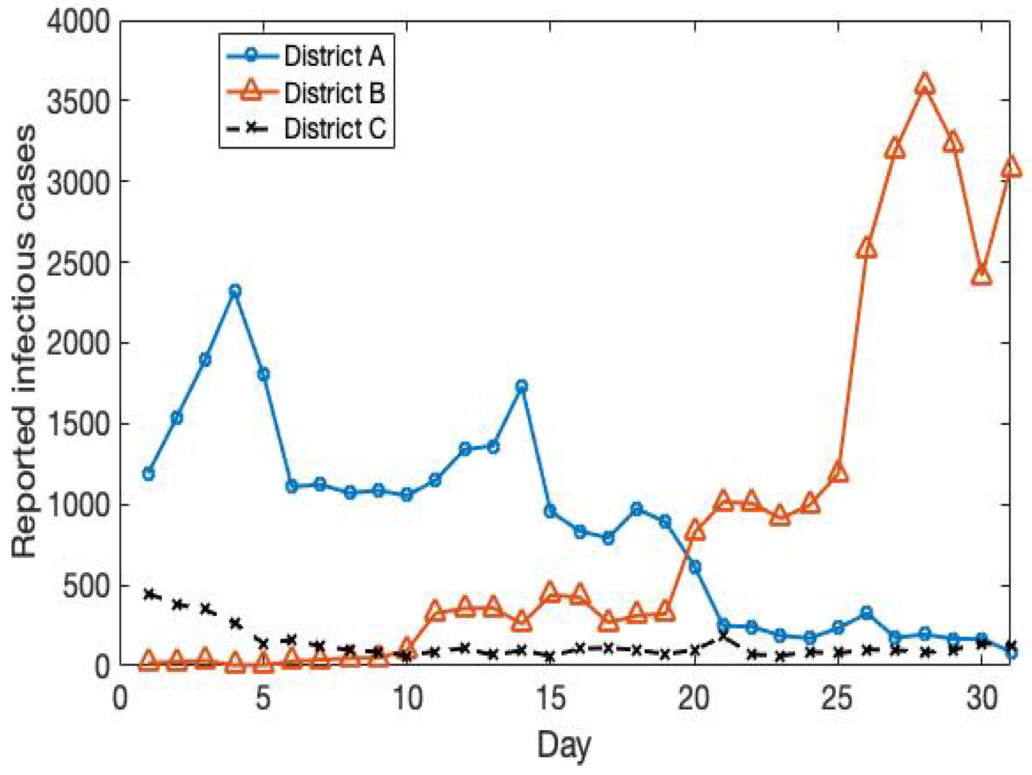
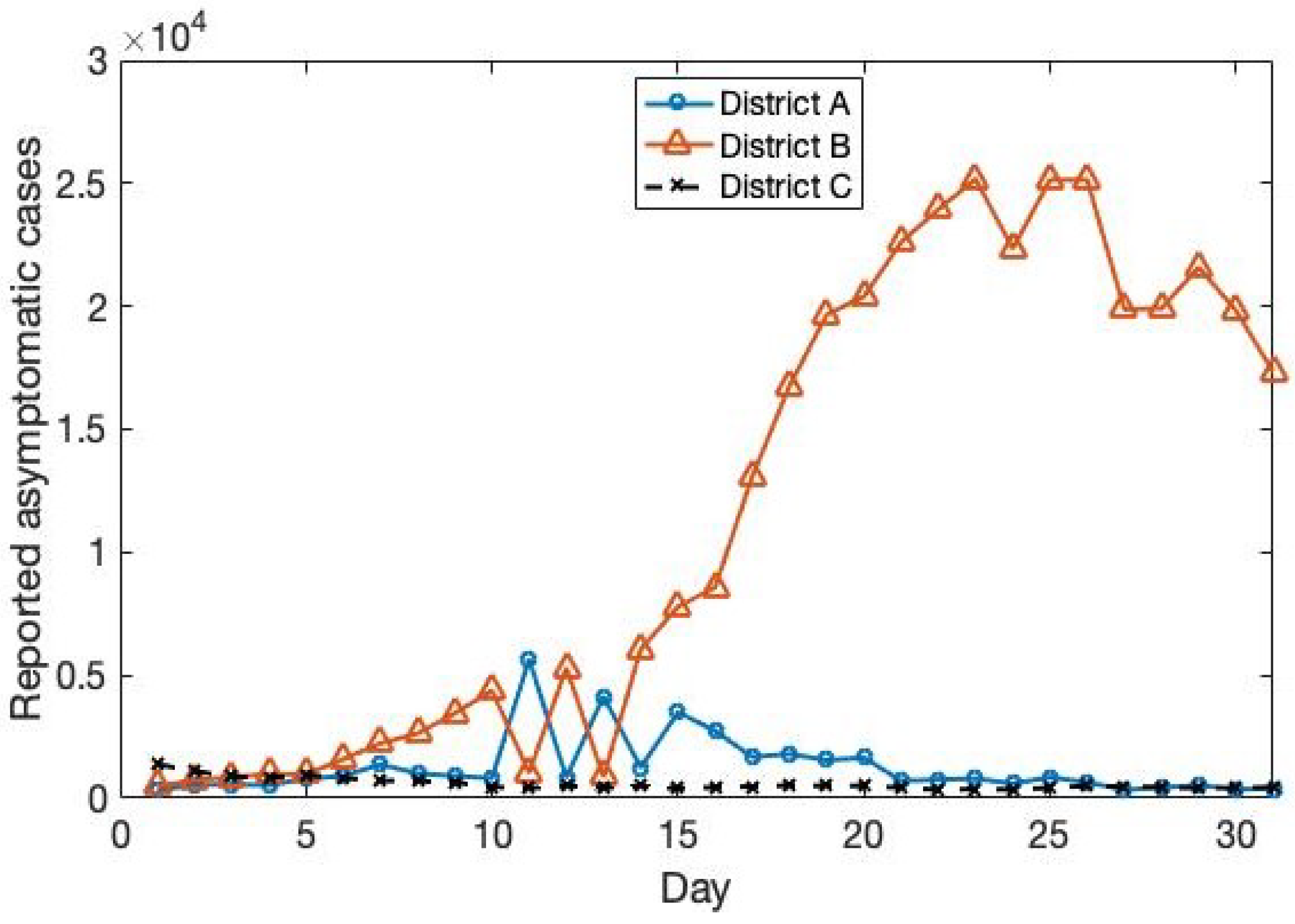
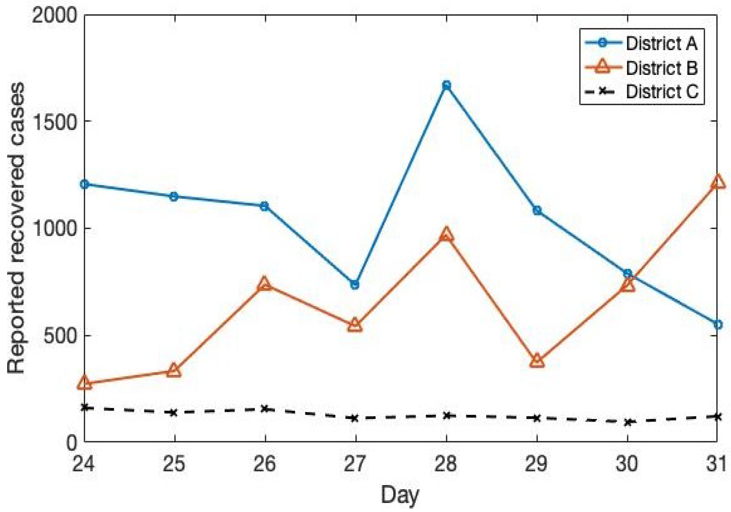
4. Numerical Simulation

In this section, the spread of the Omicron variant of COVID-19 in three districts with different characteristics will be discussed. The reported confirmed cases, asymptomatic cases, and recovered cases during a 31-day period in 2022 and the basic information of districts were collected from the Internet. The data are shown in Figure 2, Figure 3 and Figure 4.

As shown in Figure 2, Figure 3 and Figure 4, the spread of the Omicron variant of COVID-19 in District A and B is more serious than in District C. The numbers of the reported confirmed cases and asymptomatic cases in District A are reducing and the cases then flatten out. The high infection rate is a characteristic in District B during those 31 days, which means it is at the beginning of the outbreak. The numbers of the reported confirmed cases and asymptomatic cases are stable in District C. This means that the spread of the disease in District C was under control and the risk of large-scale spread is low.

The gradient descent algorithm is applied to solve the inverse problem to estimate the parameters in the model. We predict the trend of the Omicron variant of COVID-19 in different districts, based on the estimated parameters. The results are shown in Figure 5, Figure 6, Figure 7, Figure 8, Figure 9, Figure 10, Figure 11, Figure 12, Figure 13, Figure 14, Figure 15 and Figure 16.

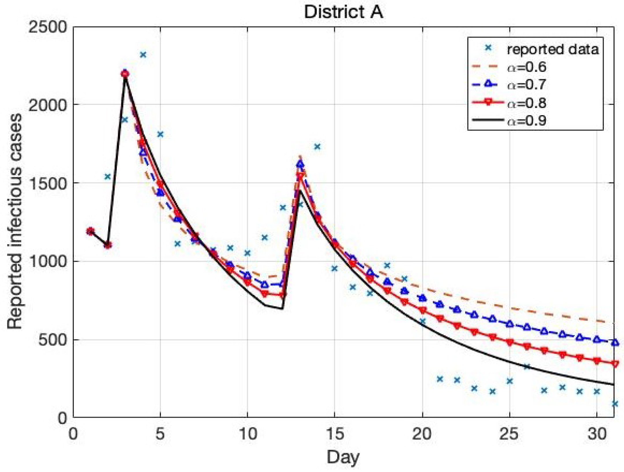
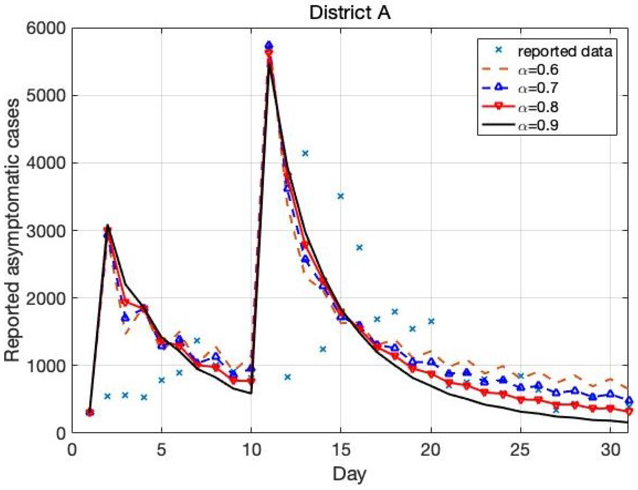
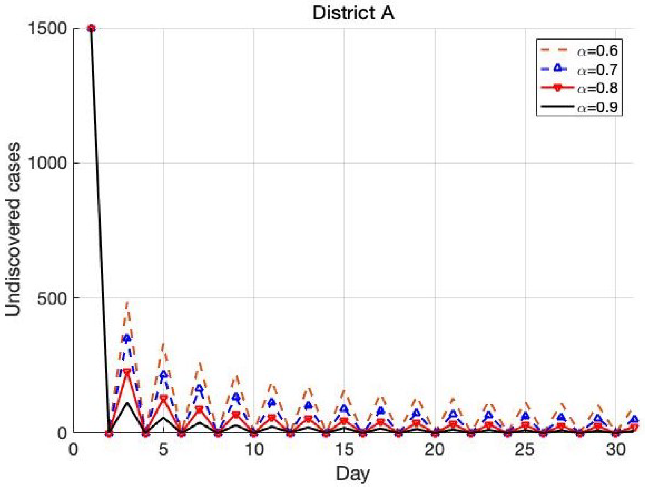
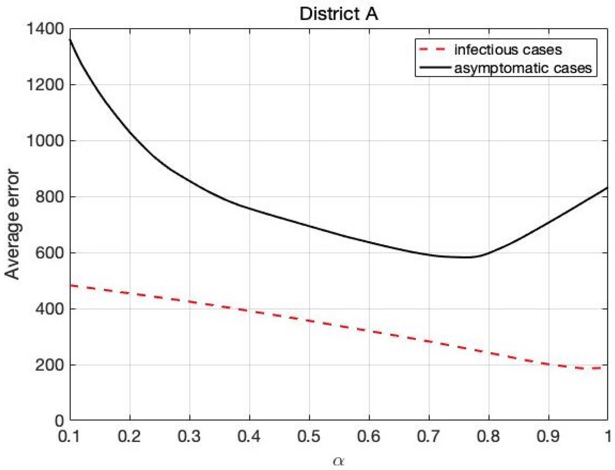
4.1. The Trend in District A

The trend of the Omicron variant of COVID-19 in District A, based on a different fractional-order, is shown in Figure 5, Figure 6, Figure 7 and Figure 8.

In Figure 6, we find there are two pulses in group I. The estimated parameters are listed as $\alpha =0.98$, ${\gamma }_3=2.5\times {10}^{-9}$, ${\gamma }_6=0.005$, ${\gamma }_7=0.05$,${\gamma }_8=0.05$, ${\gamma }_9=0.1$. In Figure 6, we find there are also two pulses in group A. The estimated parameters are listed as $\alpha =0.8$, ${\gamma }_4=2.3\times {10}^{-11}$, ${\gamma }_{10}=0.23$, ${\gamma }_{11}=1.9$. From Figure 5 and Figure 6, one can see that the numbers of class I and class A are reducing and the cases have flattened out. Figure 7 shows that the number of the undiscovered cases reduces fast. The number of undiscovered cases at the initial time is $U[1,0]=1500$. The amplitude of the oscillations becomes smaller slowly during these days. In Figure 8, we study the effect of the parameters in the model for various fractional orders. The results show that the fractional order of class A is more sensitive than that of class I. The best fractional order is $\alpha =0.78$ to describe the trend of class A, and the best fractional-order value is $\alpha =0.98$ to describe the trend of the class I.

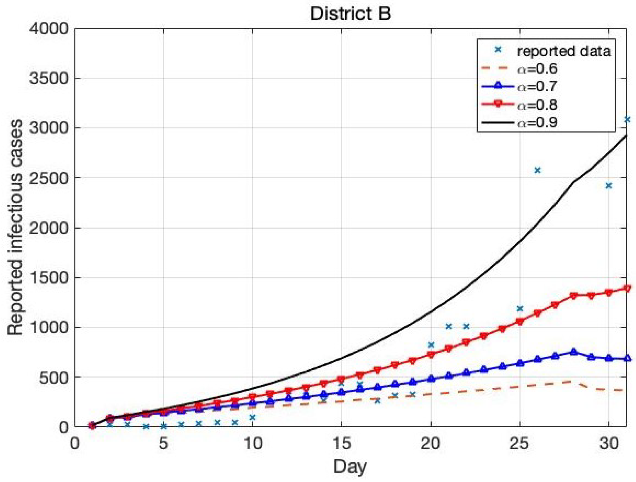
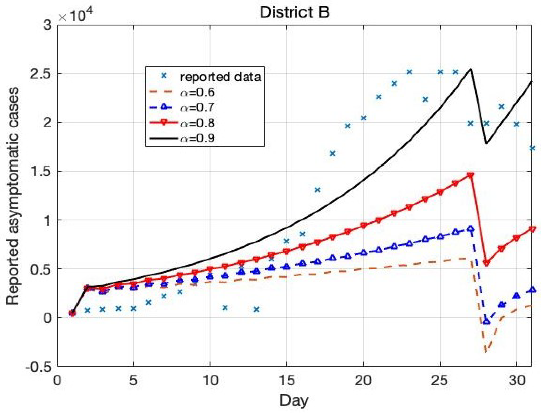
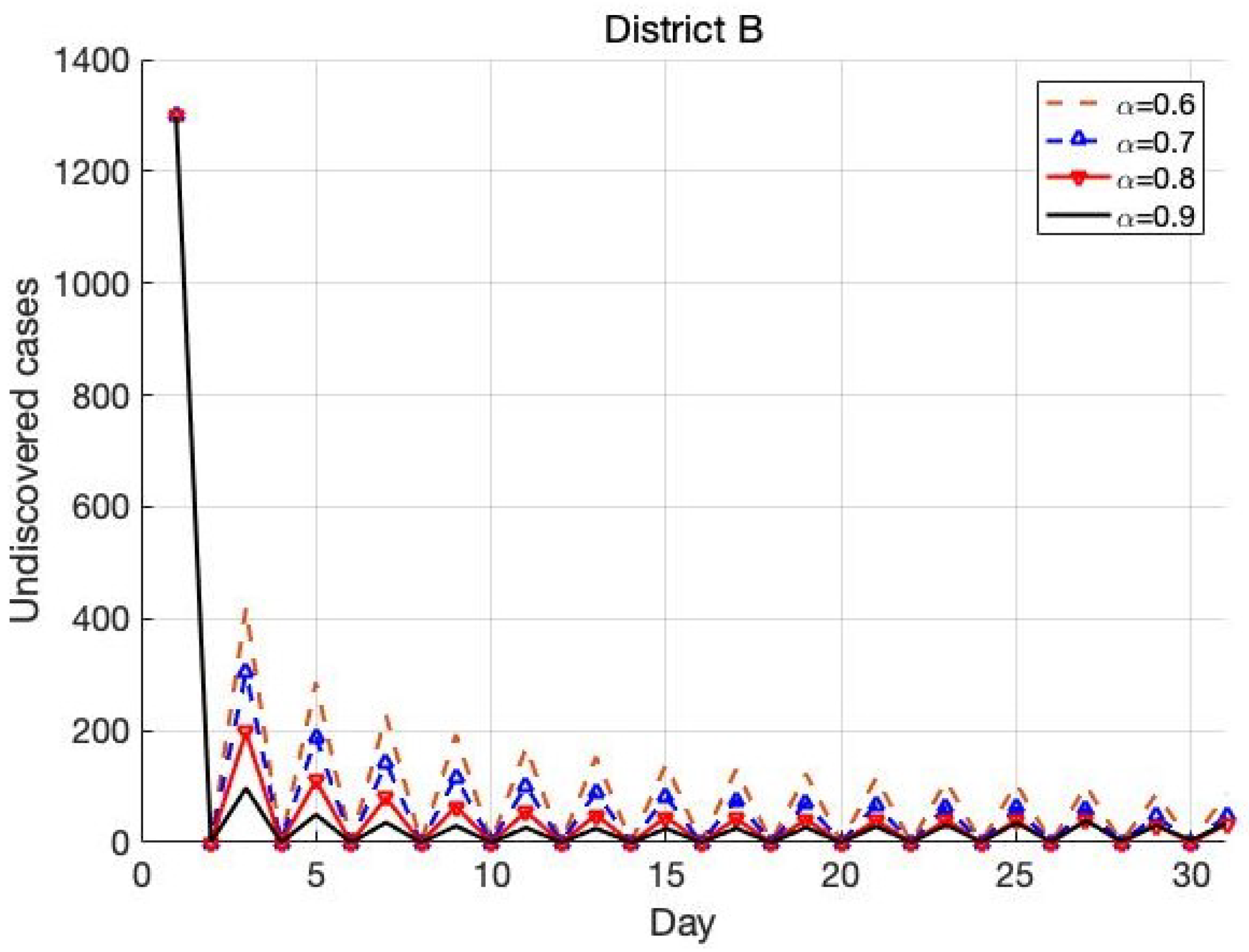
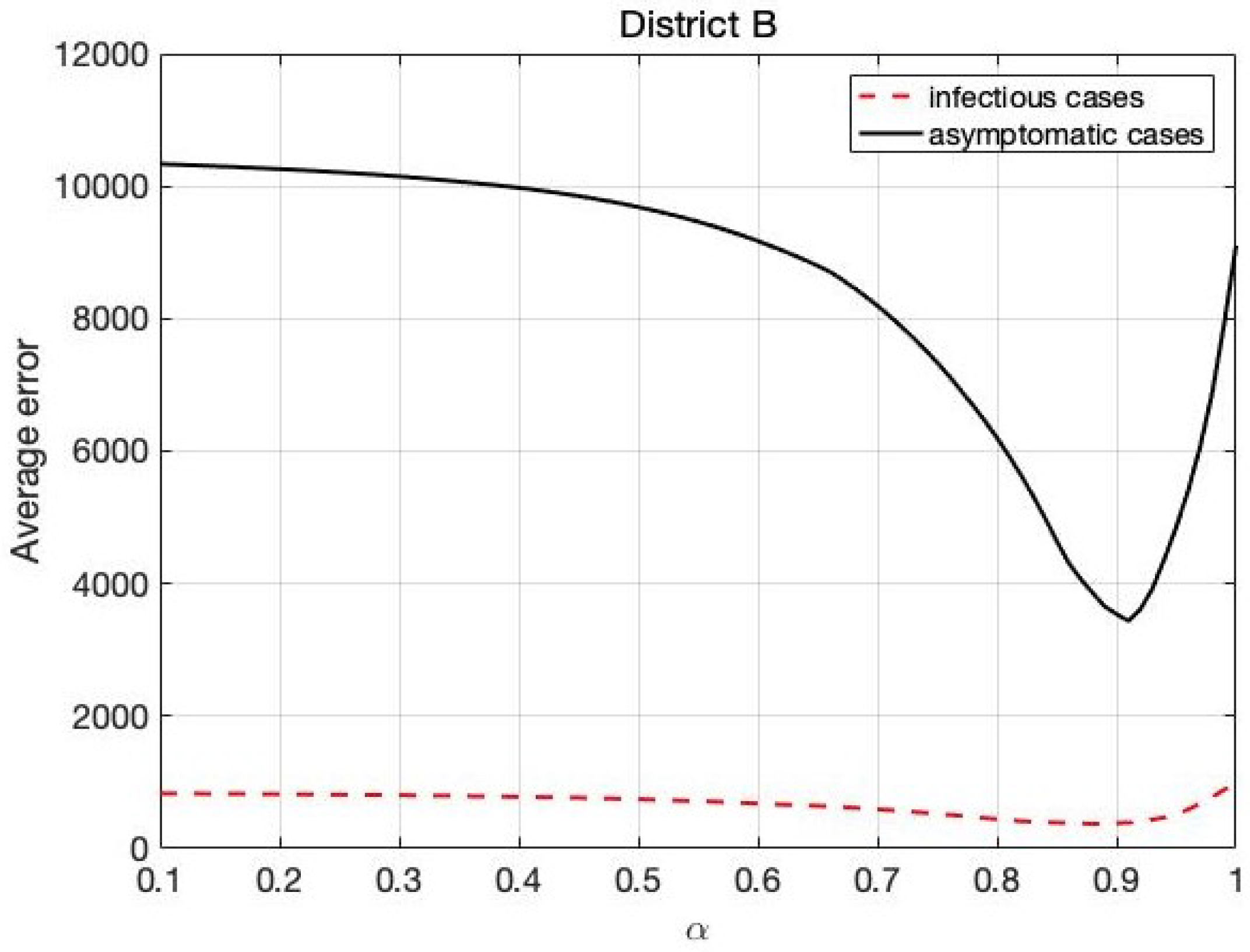
4.2. The Trend in District B

The trend of the Omicron variant of COVID-19 in District B, based on the different fractional order, is shown in Figure 9, Figure 10, Figure 11 and Figure 12.

In Figure 9, the number of class I increases during these 31 days. The estimated parameters are listed as $\alpha =0.9$, ${\gamma }_3=3.5\times {10}^{-9}$, ${\gamma }_6=0.015$, ${\gamma }_7=0.05$,${\gamma }_8=0.006$, ${\gamma }_9=0.0004$. In Figure 10, we find that there is one pulse in group A. The estimated parameters are listed as $\alpha =0.9$, ${\gamma }_4=4.3\times {10}^{-8}$, ${\gamma }_{10}=0.0009$, ${\gamma }_{11}=1.9$. From Figure 9 and Figure 10, one can see that the high infection rate is at the beginning of the outbreak. Compared with the estimated parameters obtained in District A, the spread of the Omicron variant in District B is more serious than District A. Figure 11 shows that the number of undiscovered cases is reducing fast. The amplitude of the oscillations becomes smaller slowly during these days. In Figure 12, we study the effect of the parameters in the model for various fractional-order cases. The results show that the best fractional-order value is $\alpha =0.9$ to describe the trend of class I and class A.

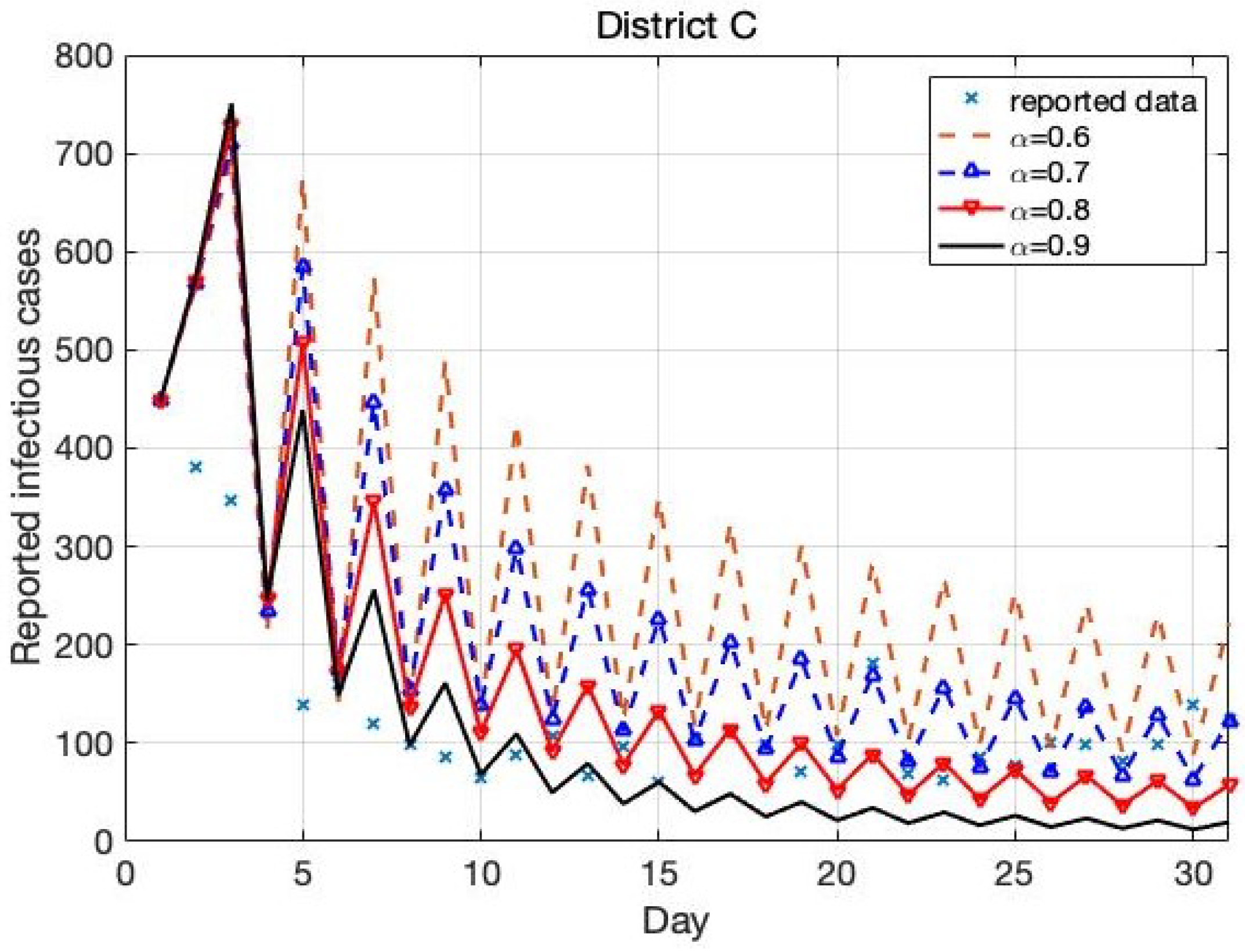
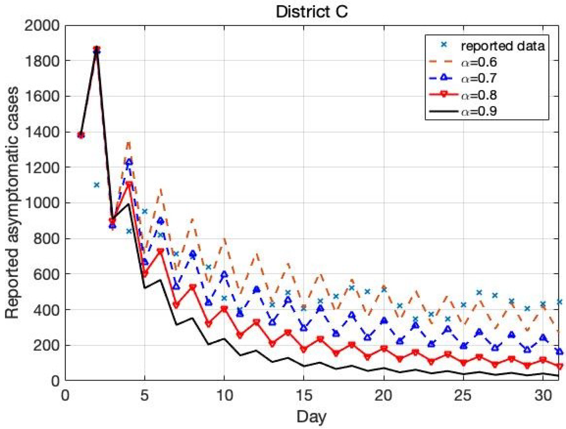
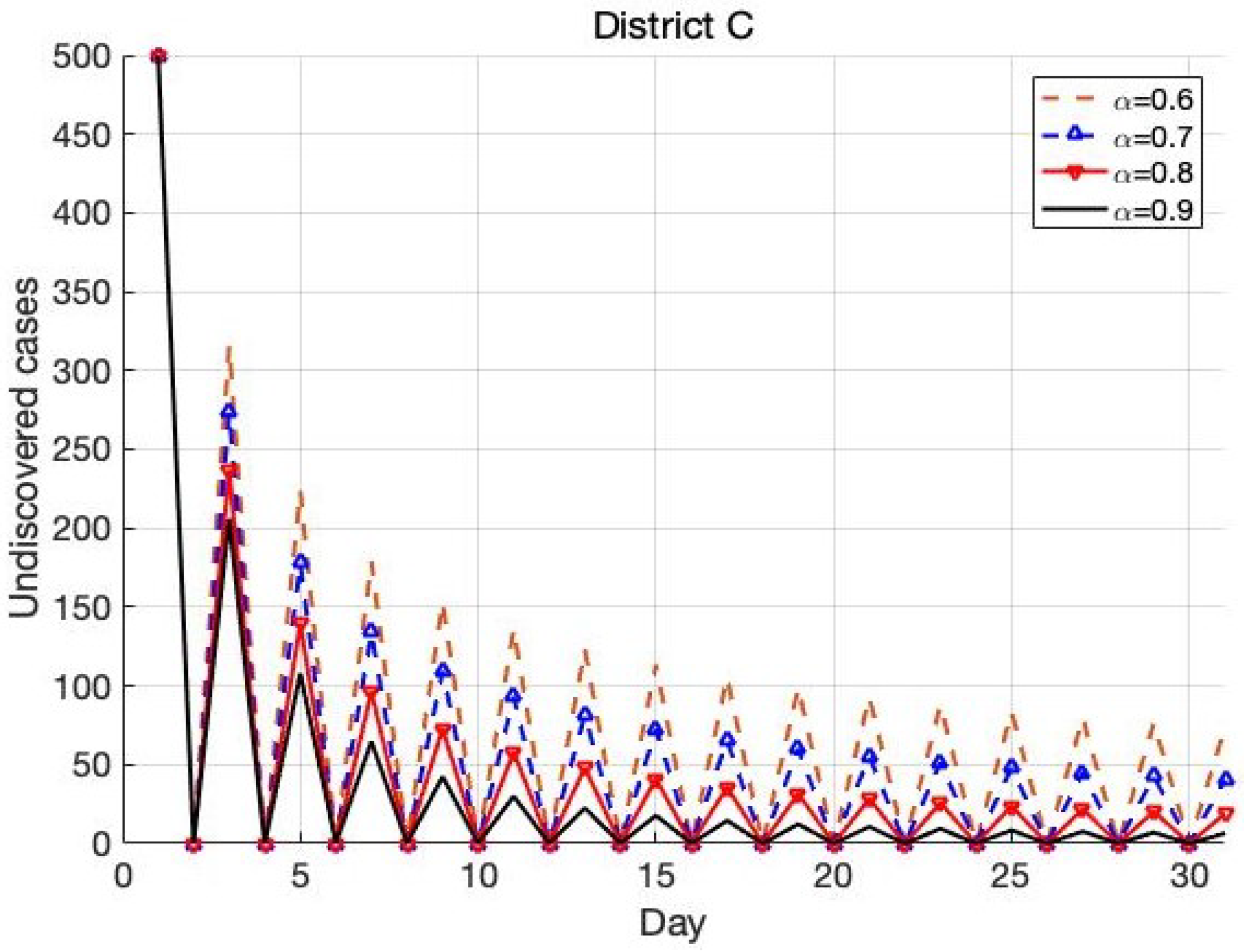
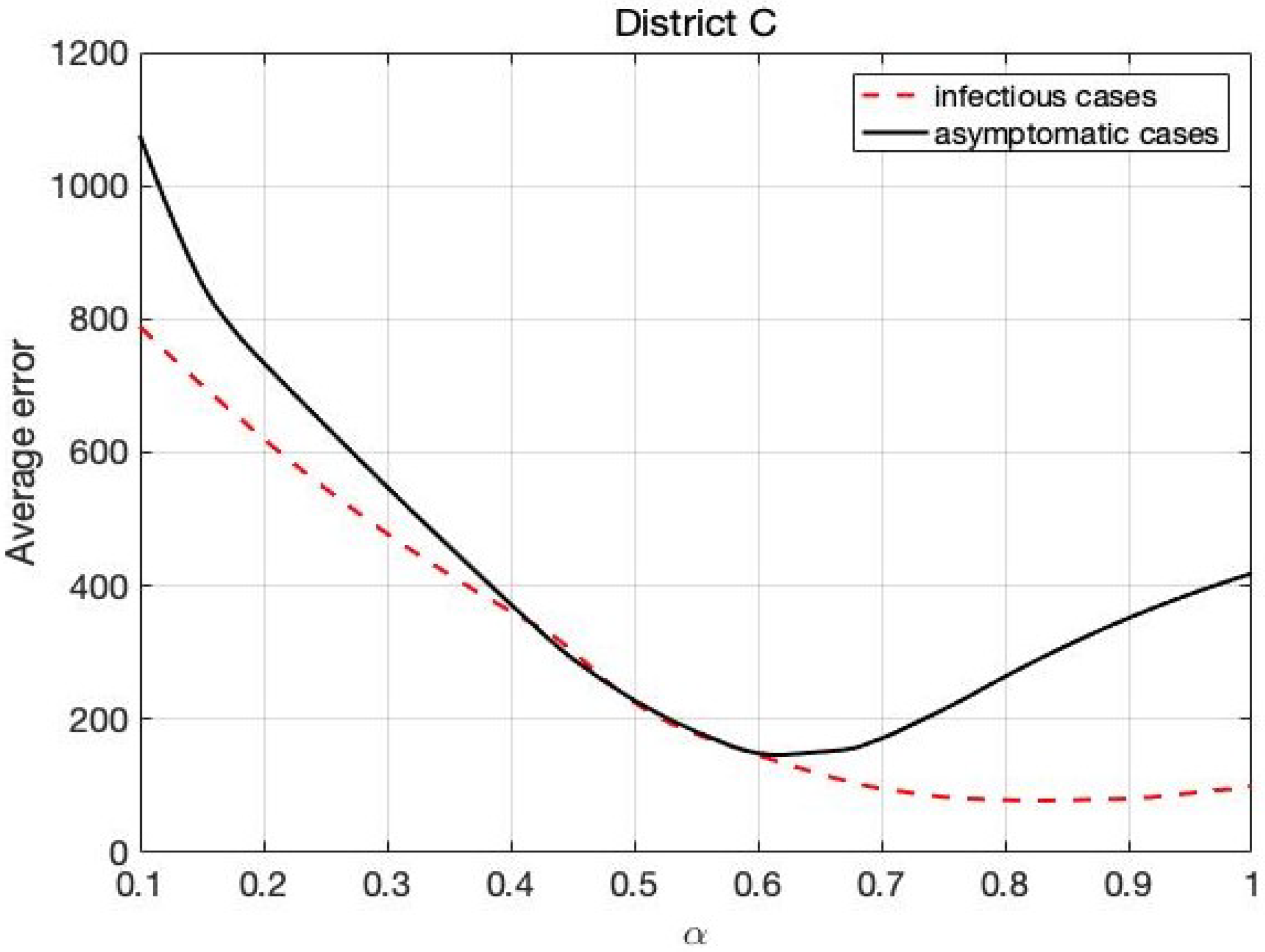
4.3. The Trend in District C

The trend of the Omicron variant of COVID-19 in District C, based on the different fractional order, is shown in Figure 13, Figure 14, Figure 15 and Figure 16.

In Figure 13, the number of class I deceases during 31 days. The estimated parameters are listed as $\alpha =0.8$, ${\gamma }_3=2.5\times {10}^{-21}$, ${\gamma }_6=0.5$, ${\gamma }_7=0.05$, ${\gamma }_8=0.6$, ${\gamma }_9=0.7$. In Figure 14, the number of class I deceases during 31 days. The estimated parameters are listed as $\alpha =0.6$, ${\gamma }_4=2.3\times {10}^{-26}$, ${\gamma }_{10}=0.023$, ${\gamma }_{11}=2.5$. Compared with the estimated parameters obtained in District A and District B, the spread of the disease in District C was under control and the risk of large-scale spread was low. Figure 15 shows that the number of the undiscovered cases is reducing fast. The number of undiscovered cases at the initial time is $U[3,0]=500$. The amplitude of the oscillations becomes smaller slowly during these days. In Figure 16, we study the effect of the parameters in the model for various fractional orders. The results show that the fractional order of class A is more sensitive than that of class I. The best fractional order is $\alpha =0.8$ to describe the trend of class A, and the best fractional order is $\alpha =0.6$ to describe the trend of class I.

5. Conclusions

In this paper, a new (2+1)-dimensional fractional-order epidemic model with pulse jumps was proposed to describe the spread of the Omicron variant of COVID-19. The problem of identifying the involved parameters in the proposed model was reduced to a minimization problem of a quadratic objective function, based on the reported data, and the approaches for analyzing the identifiability of the inverse problems were described. The main innovations in our study are using a fractional-order partial differential equation technology and considering pulse jumps in the proposed model in order to describe the characteristics and transmission mechanism of the Omicron variant of COVID-19 more accurately. The results by numerical simulation show that the degree of accuracy is higher than the corresponding classical epidemic models. By using the proposed model, the number of undiscovered cases can be calculated precisely to assess the severity of the outbreak. Three districts were considered in the paper, which are in different periods of the Omicron outbreak. At the beginning of the outbreak, there were many undiscovered cases. The infection rate was much higher than the other period. The number of reported infectious cases and asymptomatic cases increased quickly. Therefore, the regular testing protocol is very important to find the undiscovered cases. When the outbreak is under control, the risk of large-scale spread is low. The number of undiscovered cases was reducing fast. The amplitude of the oscillations became smaller slowly during these days. There are some limitations: (1) relatively small data; (2) only distance is used in the model. In future work, we will collect more data about COVID-19 to illustrate the effectiveness of our algorithm.

References

1. Shin, H.Y. A multi-stage SEIR(D) model of the COVID-19 epidemic in Korea. Ann. Med. 2021, 53, 1159–1169. [Google Scholar] [CrossRef]
2. Annas, S.; Pratama, M.I.; Rifandi, M.; Sanusi, W.; Side, S. Stability analysis and numerical simulation of SEIR model for pandemic COVID-19 spread in Indonesia. Chaos Solitons Fractals 2020, 139, 110072. [Google Scholar] [CrossRef]
3. Paul, S.; Mahata, A.; Ghosh, U.; Roy, B. Study of SEIR epidemic model and scenario analysis of COVID-19 pandemic. Ecol. Genet. Genom. 2021, 19, 100087. [Google Scholar] [CrossRef]
4. Quintero, Y.; Ardila, D.; Camargo, E.; Rivas, F.; Aguilar, J. Machine learning models for the prediction of the SEIRD variables for the COVID-19 pandemic based on a deep dependence analysis of variables. Comput. Biol. Med. 2021, 134, 104500. [Google Scholar] [CrossRef]
5. Li, J.; Zhong, J.; Ji, Y.M.; Yang, F. A new SEIAR model on small-world networks to assess the intervention measures in the COVID-19 pandemics. Results Phys. 2021, 25, 104283. [Google Scholar] [CrossRef]
6. Zhu, W.J.; Shen, S.F. An improved SIR model describing the epidemic dynamics of the COVID-19 in China. Results Phys. 2021, 25, 104289. [Google Scholar] [CrossRef]
7. Inc, M.; Acay, B.; Berhe, H.W.; Yusuf, A.; Khan, A.; Yao, S.W. Analysis of novel fractional COVID-19 model with real-life data application. Results Phys. 2021, 23, 103968. [Google Scholar] [CrossRef]
8. Omar, O.A.M.; Elbarkouky, R.A.; Ahmed, H.M. Fractional stochastic modelling of COVID-19 under wide spread of vaccinations: Egyptian case study. Alex. Eng. J. 2022, 61, 8595–8609. [Google Scholar] [CrossRef]
9. Kolebaje, O.T.; Vincent, O.R.; Vincent, U.E.; McClintock, P.V.E. Nonlinear growth and mathematical modelling of COVID-19 in some African countries with the Atangana-Baleanu fractional derivative. Commun. Nonlinear Sci. Numer. Simul. 2022, 105, 106076. [Google Scholar] [CrossRef]
10. Zhou, J.C.; Salahshour, S.; Ahmadian, A.; Senu, N. Modeling the dynamics of COVID-19 using fractal-fractional operator with a case study. Results Phys. 2022, 33, 105103. [Google Scholar] [CrossRef]
11. Omame, A.; Abbas, M.; Onyenegecha, C.P. A fractional-order model for COVID-19 and tuberculosis co-infection using Atangana-Baleanu derivative. Chaos Solitons Fractals 2021, 15, 111486. [Google Scholar] [CrossRef]
12. Omame, A.; Abbas, M.; Onyenegecha, C.P. A fractional order model for the co-interaction of COVID-19 and Hepatitis B virus. Results Phys. 2022, 37, 105498. [Google Scholar] [CrossRef]
13. Omame, A.; Isah, M.E.; Abbas, M.; Abdel-Aty, A.H.; Onyenegecha, C.P. A fractional order model for Dual Variants of COVID-19 and HIV co-infection via Atangana-Baleanu derivative. Alex. Eng. J. 2022, 61, 9715–9731. [Google Scholar] [CrossRef]
14. Meng, X.Z.; Chen, L.S.; Song, Z.T. Global dynamics behaviors for new delay SEIR epidemic disease model with vertical transmission and pulse vaccination. Appl. Math. Mech. 2007, 28, 1259–1271. [Google Scholar] [CrossRef]
15. Sekiguchi, M.; Ishiwata, E. Dynamics of a discretized SIR epidemic model with pulse vaccination and time delay. J. Comput. Appl. Math. 2011, 236, 997–1008. [Google Scholar] [CrossRef] [Green Version]
16. Ling, L.; Jiang, G.R.; Long, T.F. The dynamics of an SIS epidemic model with fixed-time birth pulses and state feedback pulse treatments. Appl. Math. Model. 2015, 39, 5579–5591. [Google Scholar] [CrossRef]
17. Asamoah, J.K.K.; Okyere, E.; Abidemi, A.; Moore, S.E.; Sun, G.Q.; Jin, Z.; Acheampong, E.; Gordon, J.F. Optimal control and comprehensive cost-effectiveness analysis for COVID-19. Results Phys. 2022, 33, 105177. [Google Scholar] [CrossRef]
18. Asamoah, J.K.K.; Jin, Z.; Sun, G.Q.; Seidu, B.; Yankson, E.; Abidemi, A.; Oduro, F.T.; Moore, S.E.; Okyere, E. Sensitivity assessment and optimal economic evaluation of a new COVID-19 compartmental epidemic model with control interventions. Chaos Solitons Fractals 2021, 146, 110885. [Google Scholar] [CrossRef]
19. Acheampong, E.; Okyere, E.; Iddi, S.; Bonney, J.H.; Asamoah, J.K.K.; Wattis, J.A.; Gomes, R.L. Mathematical modelling of earlier stages of COVID-19 transmission dynamics in Ghana. Results Phys. 2022, 34, 105193. [Google Scholar] [CrossRef]
20. Asamoah, J.K.K.; Owusu, M.A.; Jin, Z.; Oduro, F.T.; Abidemi, A.; Gyasi, E.O. Global stability and cost-effectiveness analysis of COVID-19 considering the impact of the environment: Using data from Ghana. Chaos Solitons Fractals 2020, 140, 110103. [Google Scholar]
21. Ssebuliba, J.; Nakakawa, J.N.; Ssematimba, A.; Mugisha, J.Y.T. Mathematical modelling of COVID-19 transmission dynamics in a partially comorbid community. Partial. Differ. Equ. Appl. Math. 2022, 5, 100212. [Google Scholar] [CrossRef]
22. Paul, S.; Mahata, A.; Mukherjee, S.; Roy, B. Dynamics of SIQR epidemic model with fractional order derivative. Partial. Differ. Equ. Appl. Math. 2022, 5, 100216. [Google Scholar] [CrossRef]
23. Rezapour, S.; Mohammadi, H.; Samei, M.E. SEIR epidemic model for COVID-19 transmission by Caputo derivative of fractional order. Adv. Differ. Equ. 2020, 2020, 490. [Google Scholar] [CrossRef]
24. Delshad, S.S.; Asheghan, M.M.; Beheshti, M.H. Robust stabilization of fractional-order systems with interval uncertainties via fractional-order controllers. Adv. Differ. Equ. 2010, 2010, 984601. [Google Scholar] [CrossRef] [Green Version]
25. Arenas, A.J.; Gonzlez-Parra, G.; Chen-Charpentier, B.M. Construction of nonstandard finite difference schemes for the SI and SIR epidemic models of fractional order. Math. Comput. Simul. 2016, 121, 48–63. [Google Scholar] [CrossRef]
26. Sene, N. Introduction to the fractional-order chaotic system under fractional operator in Caputo sense. Alex. Eng. J. 2021, 60, 3997–4014. [Google Scholar] [CrossRef]
Figure 1. Flow chart of the relationship between each subclasses.
Mathematics 10 02517 g001
Figure 2. The infections cases during 31 days.
Mathematics 10 02517 g002
Figure 3. The asymptomatic cases during 31 days.
Mathematics 10 02517 g003
Figure 4. The reported recovered cases during 31 days.
Mathematics 10 02517 g004
Figure 5. Model results for infected cases.
Mathematics 10 02517 g005
Figure 6. Model results for asymptomatic cases.
Mathematics 10 02517 g006
Figure 7. Model results for undiscovered cases.
Mathematics 10 02517 g007
Figure 8. Model results for various orders.
Mathematics 10 02517 g008
Figure 9. Model results for infected cases.
Mathematics 10 02517 g009
Figure 10. Model results for asymptomatic cases.
Mathematics 10 02517 g010
Figure 11. Model results for undiscovered cases.
Mathematics 10 02517 g011
Figure 12. Model results for various orders.
Mathematics 10 02517 g012
Figure 13. Model results for infected cases.
Mathematics 10 02517 g013
Figure 14. Model results for asymptomatic cases.
Mathematics 10 02517 g014
Figure 15. Model results for infected nodes.
Mathematics 10 02517 g015
Figure 16. Model results for various orders.
Mathematics 10 02517 g016