Exact Solutions and Non-Traveling Wave Solutions of the (2+1)-Dimensional Boussinesq Equation

Abstract

By the extended $(\frac{G^{\prime }}{G})$ method and the improved tanh function method, the exact solutions of the (2+1) dimensional Boussinesq equation are studied. Firstly, with the help of the solutions of the nonlinear ordinary differential equation, we obtain the new traveling wave exact solutions of the equation by the homogeneous equilibrium principle and the extended $(\frac{G^{\prime }}{G})$ method. Secondly, by constructing the new ansatz solutions and applying the improved tanh function method, many non-traveling wave exact solutions of the equation are given. The solutions mainly include hyperbolic, trigonometric and rational functions, which reflect different types of solutions for nonlinear waves. Finally, we discuss the effects of these solutions on the formation of rogue waves according to the numerical simulation.

1. Introduction

As is well known, many nonlinear phenomena can finally be described by nonlinear partial differential equations. With the wide application of nonlinear partial differential equations in practical problems, the research on solutions of high-dimensional nonlinear partial differential equations has gradually become a hot topic. There are many methods to solve the exact solution, such as Hirota’s bilinear form [1], conformable triple Sumudu decomposition method [2], Painlevé analysis [3], Exp-function method, ansatz method [4], etc. Most explicit exact solutions of equations are obtained through transformation and operation, but in fact, there is no unified solution method. Therefore, many scientists are committed to finding a universally applicable method.

A few years ago, Wang et al. in [5] used the $(\frac{G^{\prime }}{G})$-expansion method to deal with nonlinear evolution equations. The idea of this method is that the traveling wave solutions of nonlinear evolution equations can be expressed by a polynomial of $(\frac{G^{\prime }}{G})$, where $G=G(\xi )$ satisfies a linear ordinary differential equation. The degree of the polynomial can be determined by the homogeneous balance between the highest derivative term and the nonlinear term in nonlinear evolution equations, and the coefficients of the polynomial can be obtained by solving algebraic equations. Solitary waves can be derived from traveling waves, and traveling wave solutions will be expressed by hyperbolic functions, trigonometric functions and rational functions.

Furthermore, in order to find the non-traveling wave solutions of nonlinear evolution equations, Xie et al. in [6] introduced the generalized Riccati equation and then improved the tanh function method; that is, various ansatz solutions were proposed on the basis of the generalized Riccati equation. In order to show that abundant non-traveling wave solutions can be obtained by this method, they chose the (3+1)-dimensional Kadomtsev–Petviashvili equation, which can describe water waves, and finally obtained abundant soliton-like solutions, periodic solutions and rational solutions.

These two methods are concise and effective, and they can be widely used in many nonlinear evolution equations. The Boussinesq equation is a wave equation introduced by Joseph Boussinesq, which describes the dispersive and nonlinear properties of shallow water. This equation is widely applied in the research on changes in wave-induced set-up and current [7], and it is an important nonlinear partial differential equation. Many scholars have studied the exact solutions of such equations in different ways.

Song et al. in [8] gave the solitary wave number of the generalized (2+1)-dimensional Boussinesq equation, and they obtained the exact solitary wave solutions by using the bifurcation method of dynamic systems under different parameter conditions.

$$u_{tt}-\alpha u_{xx}-\beta u_{yy}-\gamma {(u^2)}_{xx}-\delta u_{xxxx}=0,$$

(1)

where $\alpha$, $\beta$, $\gamma$ and $\delta$ are arbitrary constants. Zhao et al. in [9] applied the improved $(\frac{G^{\prime }}{G})$-expansion method with a second-order linear ordinary differential equation, assuming that the form of the solution has positive and negative power terms, and they obtained the exact solutions of this equation expressed by the hyperbolic function, trigonometric function and rational function. Yang et al. in [10] used the Riccati equation to obtain abundant solutions for this equation.

When $\alpha =\beta =\gamma =\delta =1$, the generalized (2+1)-dimensional Boussinesq equation is simplified as

$$u_{tt}-u_{xx}-u_{yy}-{(u^2)}_{xx}-u_{xxxx}=0.$$

(2)

Zeng et al. in [11] have obtained the exact solutions of this equation by using Bäcklund transformation and performing mathematical calculations. Wang in [12] employed Hirota’s bilinear method and Riemann-theta functions to construct the explicit triple periodic wave solutions for this equation under the Bäcklund transformation. Liu et al. in [13] constructed a general higher-order breather solution by using Hirota’s bilinear method combined with perturbation expansion. Taking a long-wave limit for the obtained breather solution, and then making further parameter constraints, general smooth rational solutions would be succinctly constructed.

When $\alpha =\beta =\delta =1$, $\gamma =-3$, Wang et al. in [14] used the $(\frac{G^{\prime }}{G})$-expansion method to construct a new exact solution of the (2+1)-dimensional Boussinesq equation

$$u_{tt}-u_{xx}-u_{yy}+3{(u^2)}_{xx}-u_{xxxx}=0.$$

(3)

Li et al. in [15] further improved the $(\frac{G^{\prime }}{G})$-expansion method and constructed the solutions in the forms of $(\frac{G^{\prime }}{G+G^{\prime }})$ and $(\frac{G^{\prime }}{G^2})$, respectively, and they obtained and discussed the existence of the extended solution of the (2+1)-dimensional Boussinesq equation and its solution process. Jiao in [16] used the step-by-step procedure to obtain Jacobian elliptic function solutions of similarity equations, thus generating truncated series solutions of the original perturbed Boussinesq equation.

Many phenomena in nature can be simulated by functions, such as bell-shaped sech functions and kink-shaped tanh functions, which can model wave phenomena such as plasma, elastic medium, fluids, etc. [6]. In order to obtain more abundant new solutions that can explain the corresponding nonlinear phenomena, we employ the extended $(\frac{G^{\prime }}{G})$ method in [17,18] and improved the tanh function method in [19,20] to study Equation (3). In Section 2, using the solutions of nonlinear ordinary differential equation, adding the constant d, as well as positive and negative power terms, many exact solutions are constructed by the extended $(\frac{G^{\prime }}{G})$ method. Moreover, we discuss the structure and properties of the exact solutions under the same and different undetermined coefficients, and we analyze the effects of these solutions on the formation of rogue waves. In Section 3, by using the improved tanh function method, constructing new ansatz solutions of the generalized Riccati equation, and assuming that the solution has a positive power term and negative power term, we obtain three groups of non-traveling wave solutions composed of arbitrary functions $\mu (y,t)$ and $c(y,t)$. Furthermore, we discuss the different trajectories of the image in a certain direction for different differentiable functions. In Section 4, some conclusions are given.

2. Extended $(\frac{{\mathit{G}}^{\prime }}{\mathit{G}})$ Method

2.1. Preliminary

The extended $(\frac{G^{\prime }}{G})$ method is based on the general method, changing the auxiliary nonlinear ordinary differential equations and undetermined functions. For a given nonlinear partial differential equation

$$P(u,u_t,u_x,u_{tt},u_{xt},u_{xx},\dots )=0,$$

(4)

the main steps of the extended $(\frac{G^{\prime }}{G})$ method are as follows.

Step 1

Making the traveling wave transformation on Equation (4), we suppose that $u(\xi )=u(x,y,\dots ,t)$, $\xi =a_{1}x+a_{2}y+\dots -bt$, in which $a_j(j=1,2,\dots )$ and b are undetermined real constants. Then, we integrate and simplify it to an ordinary differential equation

$$P(e,u,u^{\prime },u^{″},\dots )=0,$$

(5)

where e is a integral constant, and $u^{\prime }=\frac{du}{d\xi },u^{″}=\frac{d^{2}u}{d{\xi }^2},\dots$

Step 2

Supposing that the solution of Equation (5) has the following form

$$u(\xi )=\sum _{i=-N}^N{e}_i{(d+H(\xi ))}^i,$$

(6)

where $e_i$ $(i=0,\pm 1,\pm 2,\dots ,\pm N)$$(i=0,1,2,\dots ,N)$ are undetermined constants and $e_i\ne 0$, N is determined by the homogeneous balance principle, and $H(\xi )=\frac{G^{\prime }(\xi )}{G(\xi )}$ satisfies an auxiliary nonlinear partial differential equation of G.

Step 3

Substituting (6) into Equation (5), we use the auxiliary equation to convert the left-hand side of Equation (5) into a polynomial of $(d+H(\xi ))$. Equating each coefficient of the same power term of $(d+H(\xi ))$ to zero, then we obtain the algebraic equations about undetermined coefficients.

Step 4

Solving the algebraic equations of $e_i$$(i=0,\pm 1,\pm 2,\dots ,\pm N)$$(i=0,\pm 1,\pm 2,\dots ,\pm N)$ and e, we finally substitute the solutions of the auxiliary equation to determine the specific form of (6).

The choice of auxiliary equations determines the structure and properties of solutions of nonlinear partial differential equation. Generally speaking, the $(\frac{G^{\prime }}{G})$-expansion method in [14] is to use a second-order linear ordinary differential equation $G^{″}+\lambda G^{\prime }+\mu G=0$, which includes three types of solutions.

In Ref. [21], the author mentioned a nonlinear auxiliary ordinary differential equation

$$AG{G}^{″}-BG{G}^{\prime }-C{(G^{\prime })}^2-E{G}^2=0,$$

(7)

where A, B, C and E are undermined coefficients. Taking $M=A-C$, $\omega =B^2+4EM$, and $\Delta =ME$, the solutions of this equation are as follows.

When $B\ne 0$ and $\omega >0$,

$$H(\xi )=(\frac{G^{\prime }}{G})=\frac{B}{2M}+\frac{\sqrt{\omega }}{2M}\frac{C_{1}sinh(\frac{\sqrt{\omega }}{2A}\xi )-C_{2}cosh(\frac{\sqrt{\omega }}{2A}\xi )}{C_{2}sinh(\frac{\sqrt{\omega }}{2A}\xi )+C_{1}cosh(\frac{\sqrt{\omega }}{2A}\xi )}.$$

(8)

When $B\ne 0$ and $\omega <0$,

$$H(\xi )=(\frac{G^{\prime }}{G})=\frac{B}{2M}+\frac{\sqrt{-\omega }}{2M}\frac{-C_{1}sin(\frac{\sqrt{-\omega }}{2A}\xi )+C_{2}cos(\frac{\sqrt{-\omega }}{2A}\xi )}{C_{2}sin(\frac{\sqrt{-\omega }}{2A}\xi )+C_{1}cos(\frac{\sqrt{-\omega }}{2A}\xi )}.$$

(9)

When $B\ne 0$ and $\omega =0$,

$$H(\xi )=(\frac{G^{\prime }}{G})=\frac{B}{2M}+\frac{C_2}{C_1+C_2\xi }.$$

(10)

When $B=0$ and $\Delta >0$,

$$H(\xi )=(\frac{G^{\prime }}{G})=\frac{\sqrt{\Delta }}{M}\frac{C_{1}sinh(\frac{\sqrt{\Delta }}{A}\xi )+C_{2}cosh(\frac{\sqrt{\Delta }}{A}\xi )}{C_{2}sinh(\frac{\sqrt{\Delta }}{A}\xi )-C_{1}cosh(\frac{\sqrt{\Delta }}{A}\xi )}.$$

(11)

When $B=0$ and $\Delta <0$,

$$H(\xi )=(\frac{G^{\prime }}{G})=\frac{\sqrt{-\Delta }}{M}\frac{-C_{1}sin(\frac{\sqrt{-\Delta }}{A}\xi )+C_{2}cos(\frac{\sqrt{-\Delta }}{A}\xi )}{C_{2}sin(\frac{\sqrt{-\Delta }}{A}\xi )+C_{1}cos(\frac{\sqrt{-\Delta }}{A}\xi )}.$$

(12)

In the subsequent sections, we will use the extended $(\frac{G^{\prime }}{G})$ method to solve the exact solutions of (2+1)-dimensional Boussinesq equation with $AG{G}^{″}-BG{G}^{\prime }-C{(G^{\prime })}^2-E{G}^2=0$ as an auxiliary equation.

2.2. Expression Form of Traveling Wave Solution

Considering the following (2+1)-dimensional Boussinesq equation

$$u_{tt}-u_{xx}-u_{yy}+3{(u^2)}_{xx}-u_{xxxx}=0,$$

through traveling wave transformation $u(\xi )=u(x,y,t)$, $\xi =x+ay-bt,$ where $a,b$ are two non-zero constants, Equation (3) becomes

$$(b^2-1-a^2)u^{″}+3{(u^2)}^{″}-u^{⁗}=0.$$

Integrating it twice, we obtain

$$u^{″}-3u^2+cu+e=0,$$

(13)

where e is a real integral constant, $c=a^2+1-b^2$. We suppose Supposingthat Equation (13) has the following solution

$$u(\xi )=\sum _{i=-N}^N{e}_i{(d+H(\xi ))}^i.$$

(14)

When whenthe power of the highest-order derivative term $u^{″}$ and the nonlinear term $u^2$ are equal, then $N=2$. Furthermore, (14) can be written as

$$u(\xi )=e_{-2}{(d+H)}^{-2}+e_{-1}{(d+H)}^{-1}+e_0+e_1(d+H)+e_2{(d+H)}^2.$$

(15)

Substituting (15) into Equation (13), and taking $\mathsf{\Theta }=M{d}^2+Bd-E$, then we obtain the following algebraic equations about undetermined coefficients.

$$\left\{\begin{array}{c}-3A^2{e}_2(e_2-{\displaystyle \frac{2M^2}{A^2}})=0,\hfill \\ -6A^2(e_2-{\displaystyle \frac{2M^2}{A^2}})((e_1+{\displaystyle \frac{2M(2dM+B)}{A^2}}))-10M^2(e_1+{\displaystyle \frac{2M(2dM+B)}{A^2}})=0,\hfill \\ 3A^2({\displaystyle \frac{M(B+2dM)}{A^2}}-e_1)(e_1+{\displaystyle \frac{2M(B+2dM)}{A^2}})-12M^2(e_0-{\displaystyle \frac{12M\mathsf{\Theta }+A^{2}c+\omega }{6A^2}})\hfill \\ +6A^2(e_2-{\displaystyle \frac{2M^2}{A^2}})(({\displaystyle \frac{12M\mathsf{\Theta }+A^{2}c+\omega }{6A^2}}-e_0)+{\displaystyle \frac{{(B+2dM)}^2}{2A^2}})=0,\hfill \\ -6A^2(e_2-{\displaystyle \frac{2M^2}{A^2}})(e_{-1}+{\displaystyle \frac{\mathsf{\Theta }(B+2dM)}{A^2}})-6M\mathsf{\Theta }(e_1+{\displaystyle \frac{2M(B+2dM)}{A^2}})\hfill \\ -12M^2{e}_{-1}=0,\hfill \\ A^2{e}_0(c+3e_0+e)-6A^2(e_2{e}_{-2}+e_1{e}_{-1})+2M^2{e}_{-2}+2e_2{\mathsf{\Theta }}^2-e_1(B+2dM)\mathsf{\Theta }\hfill \\ -e_{-1}M(B+2dM)=0,\hfill \\ -6A^2(e_{-2}-{\displaystyle \frac{2{\mathsf{\Theta }}^2}{A^2}})(e_1+{\displaystyle \frac{M(B+2dM)}{A^2}})-6M\mathsf{\Theta }(e_{-1}+{\displaystyle \frac{2(B+2dM)\mathsf{\Theta }}{A^2}})\hfill \\ -12{\mathsf{\Theta }}^2{e}_1=0,\hfill \\ 3A^2(e_{-1}+{\displaystyle \frac{2(B+2dM)\mathsf{\Theta }}{A^2}})({\displaystyle \frac{(B+2dM)\mathsf{\Theta }}{A^2}}-e_{-1}))-12\mathsf{\Theta }(e_0-{\displaystyle \frac{12M\mathsf{\Theta }+A^{2}c+\omega }{6A^2}})\hfill \\ +6A^2(e_{-2}-{\displaystyle \frac{2{\mathsf{\Theta }}^2}{A^2}})(({\displaystyle \frac{12M\mathsf{\Theta }+A^{2}c+\omega }{6A^2}}-e_0)+{\displaystyle \frac{{(B+2dM)}^2}{2A^2}})=0,\hfill \\ -6A^2(e_{-2}-{\displaystyle \frac{2{\mathsf{\Theta }}^2}{A^2}})(e_{-1}+{\displaystyle \frac{5(B+2dM)\mathsf{\Theta }}{3A^2}})+10{\mathsf{\Theta }}^2(e_{-1}+{\displaystyle \frac{2(B+2dM)\mathsf{\Theta }}{A^2}})=0,\hfill \\ -3A^2{e}_{-2}(e_{-2}-{\displaystyle \frac{2{\mathsf{\Theta }}^2}{A^2}})=0.\hfill \end{array}\right.$$

By solving these equations with Maple math software, we obtain three groups of coefficient relations about $e_{-2}$, $e_{-1}$, $e_0$, $e_1$, $e_2$ and e.

Group 1

$$e=\frac{{\omega }^2-A^4{c}^2}{12A^4},e_{-2}=0,e_{-1}=0,$$

$$e_0=\frac{12M(M{d}^2+Bd-E)+A^{2}c+\omega }{6A^2},e_1=-\frac{2M(2dM+B)}{A^2},e_2=\frac{2M^2}{A^2}.$$

Group 2

$$e=\frac{{\omega }^2-A^4{c}^2}{12A^4},e_{-2}=\frac{2{(M{d}^2+Bd-E)}^2}{A^2},e_{-1}=-\frac{2(2dM+B)(M{d}^2+Bd-E)}{A^2},$$

$$e_0=\frac{12M(M{d}^2+Bd-E)+A^{2}c+\omega }{6A^2},e_1=0,e_2=0.$$

Group 3

$$e=\frac{256M^2{(M{d}^2+E)}^2-A^4{c}^2}{12A^4},e_{-2}=\frac{2{(M{d}^2+E)}^2}{A^2},e_{-1}=0,$$

$$e_0=\frac{A^{2}c-8M(M{d}^2+E)}{6A^2},e_1=0,e_2=\frac{2M^2}{A^2},B=-2dM.$$

Considering the exact solutions of each group when the conditions (8)–(12) are satisfied, for convenience, in (8) and (11), $C_1^2-C_2^2=1$, $C_3=\mathrm{arccosh}{C}_1=\mathrm{arcsinh}{C}_2.$ In (10), $C_2\ne 0$, $C_3=\frac{C_1}{C_2}.$ In (9) and (12), $C_1^2+C_2^2=1$, $C_3=$arccos$C_1=$arcsin$C_2.$

The exact solutions of Group 1 are as follows.

$u_{1,1}(\xi )={\displaystyle \frac{12M(M{d}^2+Bd-E)+A^{2}c+\omega }{6A^2}}$

$-{\displaystyle \frac{2M(2dM+B)}{A^2}}(d+{\displaystyle \frac{B}{2M}}+{\displaystyle \frac{\sqrt{\omega }}{2M}}tanh({\displaystyle \frac{\sqrt{\omega }}{2A}}\xi -C_3))$

$+{\displaystyle \frac{2M^2}{A^2}}{(d+{\displaystyle \frac{B}{2M}}+{\displaystyle \frac{\sqrt{\omega }}{2M}}tanh({\displaystyle \frac{\sqrt{\omega }}{2A}}\xi -C_3))}^2,$

$u_{1,2}(\xi )={\displaystyle \frac{12M(M{d}^2+Bd-E)+A^{2}c+\omega }{6A^2}}$

$-{\displaystyle \frac{2M(2dM+B)}{A^2}}(d+{\displaystyle \frac{B}{2M}}+{\displaystyle \frac{\sqrt{-\omega }}{2M}}tan(-{\displaystyle \frac{\sqrt{-\omega }}{2A}}\xi +C_3))$

$+{\displaystyle \frac{2M^2}{A^2}}{(d+{\displaystyle \frac{B}{2M}}+{\displaystyle \frac{\sqrt{-\omega }}{2M}}tan(-{\displaystyle \frac{\sqrt{-\omega }}{2A}}\xi +C_3))}^2,$

$u_{1,3}(\xi )={\displaystyle \frac{12M(M{d}^2+Bd-E)+A^{2}c+\omega }{6A^2}}-{\displaystyle \frac{2M(2dM+B)}{A^2}}(d+{\displaystyle \frac{B}{2M}}+{\displaystyle \frac{1}{\xi +C_3}})$

$+{\displaystyle \frac{2M^2}{A^2}}{(d+{\displaystyle \frac{B}{2M}}+{\displaystyle \frac{1}{\xi +C_3}})}^2,$

$u_{1,4}(\xi )={\displaystyle \frac{12M^2{d}^2-8ME+A^{2}c}{6A^2}}+{\displaystyle \frac{2M^2}{A^2}}{(d+{\displaystyle \frac{\sqrt{\Delta }}{M}}tanh({\displaystyle \frac{\sqrt{\Delta }}{A}}\xi +C_3))}^2$

$-{\displaystyle \frac{4M^{2}d}{A^2}}(d+{\displaystyle \frac{\sqrt{\Delta }}{M}}tanh({\displaystyle \frac{\sqrt{\Delta }}{A}}\xi +C_3)),$

$u_{1,5}(\xi )={\displaystyle \frac{12M^2{d}^2-8ME+A^{2}c}{6A^2}}+{\displaystyle \frac{2M^2}{A^2}}{(d+{\displaystyle \frac{\sqrt{-\Delta }}{M}}tan(-{\displaystyle \frac{\sqrt{-\Delta }}{A}}\xi +C_3))}^2$

$-{\displaystyle \frac{4M^{2}d}{A^2}}(d+{\displaystyle \frac{\sqrt{-\Delta }}{M}}tan(-{\displaystyle \frac{\sqrt{-\Delta }}{A}}\xi +C_3)).$

The exact solutions of Group 2 are as follows.

$u_{2,1}(\xi )={\displaystyle \frac{12M(M{d}^2+Bd-E)+A^{2}c+\omega }{6A^2}}$

$-{\displaystyle \frac{2(2dM+B)(M{d}^2+Bd-E)}{A^2}}{(d+{\displaystyle \frac{B}{2M}}+{\displaystyle \frac{\sqrt{\omega }}{2M}}tanh({\displaystyle \frac{\sqrt{\omega }}{2A}}\xi -C_3))}^{-1}$

$+{\displaystyle \frac{2{(M{d}^2+Bd-E)}^2}{A^2}}{(d+{\displaystyle \frac{B}{2M}}+{\displaystyle \frac{\sqrt{\omega }}{2M}}tanh({\displaystyle \frac{\sqrt{\omega }}{2A}}\xi -C_3))}^{-2},$

$u_{2,2}(\xi )={\displaystyle \frac{12M(M{d}^2+Bd-E)+A^{2}c+\omega }{6A^2}}$

$-{\displaystyle \frac{2(2dM+B)(M{d}^2+Bd-E)}{A^2}}{(d+{\displaystyle \frac{B}{2M}}+{\displaystyle \frac{\sqrt{-\omega }}{2M}}tan(-{\displaystyle \frac{\sqrt{-\omega }}{2A}}\xi +C_3))}^{-1}$

$+{\displaystyle \frac{2{(M{d}^2+Bd-E)}^2}{A^2}}{(d+{\displaystyle \frac{B}{2M}}+{\displaystyle \frac{\sqrt{-\omega }}{2M}}tan(-{\displaystyle \frac{\sqrt{-\omega }}{2A}}\xi +C_3))}^{-2},$

$u_{2,3}(\xi )={\displaystyle \frac{12M(M{d}^2+Bd-E)+A^{2}c+\omega }{6A^2}}$

$-{\displaystyle \frac{2(2dM+B)(M{d}^2+Bd-E)}{A^2}}{(d+{\displaystyle \frac{B}{2M}}+{\displaystyle \frac{1}{\xi +C_3}})}^{-1}$

$+{\displaystyle \frac{2{(M{d}^2+Bd-E)}^2}{A^2}}{(d+{\displaystyle \frac{B}{2M}}+{\displaystyle \frac{1}{\xi +C_3}})}^{-2},$

$u_{2,4}(\xi )={\displaystyle \frac{12M^2{d}^2-8ME+A^{2}c}{6A^2}}+{\displaystyle \frac{2{(M{d}^2-E)}^2}{A^2}}{(d+{\displaystyle \frac{\sqrt{\Delta }}{M}}tanh({\displaystyle \frac{\sqrt{\Delta }}{A}}\xi +C_3))}^{-2}$

$-{\displaystyle \frac{4dM(M{d}^2-E)}{A^2}}{(d+{\displaystyle \frac{\sqrt{\Delta }}{M}}tanh({\displaystyle \frac{\sqrt{\Delta }}{A}}\xi +C_3))}^{-1},$

$u_{2,5}(\xi )={\displaystyle \frac{12M^2{d}^2-8ME+A^{2}c}{6A^2}}$

$-{\displaystyle \frac{4dM(M{d}^2-E)}{A^2}}{(d+{\displaystyle \frac{\sqrt{-\Delta }}{M}}tan(-{\displaystyle \frac{\sqrt{-\Delta }}{A}}\xi +C_3))}^{-1}$

$+{\displaystyle \frac{2{(M{d}^2-E)}^2}{A^2}}{(d+{\displaystyle \frac{\sqrt{-\Delta }}{M}}tan(-{\displaystyle \frac{\sqrt{-\Delta }}{A}}\xi +C_3))}^{-2}.$

The exact solutions of Group 3 are as follows.

$u_{3,1}(\xi )={\displaystyle \frac{A^{2}c-8M(M{d}^2+E)}{6A^2}}+{\displaystyle \frac{2M^2}{A^2}}{({\displaystyle \frac{\sqrt{\omega }}{2M}}tanh({\displaystyle \frac{\sqrt{\omega }}{2A}}\xi -C_3))}^2$

$+{\displaystyle \frac{2{(M{d}^2+E)}^2}{A^2}}{({\displaystyle \frac{\sqrt{\omega }}{2M}}tanh({\displaystyle \frac{\sqrt{\omega }}{2A}}\xi -C_3))}^{-2},$

$u_{3,2}(\xi )={\displaystyle \frac{A^{2}c-8M(M{d}^2+E)}{6A^2}}+{\displaystyle \frac{2M^2}{A^2}}{({\displaystyle \frac{\sqrt{-\omega }}{2M}}tan(-{\displaystyle \frac{\sqrt{-\omega }}{2A}}\xi +C_3))}^2$

$+{\displaystyle \frac{2{(M{d}^2+E)}^2}{A^2}}{({\displaystyle \frac{\sqrt{-\omega }}{2M}}tan(-{\displaystyle \frac{\sqrt{-\omega }}{2A}}\xi +C_3))}^{-2},$

$u_{3,3}(\xi )={\displaystyle \frac{A^{2}c-8M(M{d}^2+E)}{6A^2}}+{\displaystyle \frac{2M^2}{A^2}}{({\displaystyle \frac{1}{\xi +C_3}})}^2+{\displaystyle \frac{2{(M{d}^2+E)}^2}{A^2}}{({\displaystyle \frac{1}{\xi +C_3}})}^{-2},$

$u_{3,4}(\xi )={\displaystyle \frac{A^{2}c-8ME}{6A^2}}+{\displaystyle \frac{2M^2}{A^2}}{({\displaystyle \frac{\sqrt{\Delta }}{M}}tanh({\displaystyle \frac{\sqrt{\Delta }}{A}}\xi +C_3))}^2$

$+{\displaystyle \frac{2E^2}{A^2}}{({\displaystyle \frac{\sqrt{\Delta }}{M}}tanh({\displaystyle \frac{\sqrt{\Delta }}{A}}\xi +C_3))}^{-2},$

$u_{3,5}(\xi )={\displaystyle \frac{A^{2}c-8ME}{6A^2}}+{\displaystyle \frac{2M^2}{A^2}}{({\displaystyle \frac{\sqrt{-\Delta }}{M}}tan(-{\displaystyle \frac{\sqrt{-\Delta }}{A}}\xi +C_3))}^2$

$+{\displaystyle \frac{2E^2}{A^2}}{({\displaystyle \frac{\sqrt{-\Delta }}{M}}tan(-{\displaystyle \frac{\sqrt{-\Delta }}{A}}\xi +C_3))}^{-2}.$

Next, we numerically simulate the solutions, and the images are shown in Figure 1, Figure 2, Figure 3, Figure 4, Figure 5, Figure 6, Figure 7, Figure 8, Figure 9, Figure 10, Figure 11, Figure 12 and Figure 13, where $r=x-\frac{t}{2}$, w $\omega$$=y-\frac{t}{2}$.

2.3. Numerical Simulation of Solutions under Different Undetermined Coefficient Values

Firstly, we discuss the structure and properties of the exact solutions under different undetermined coefficient values.

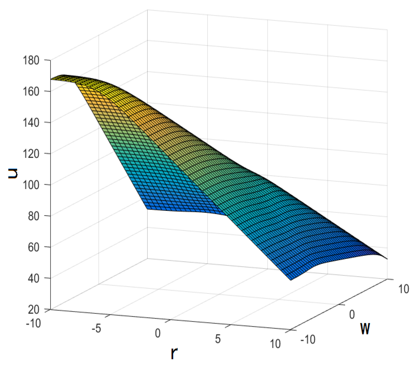
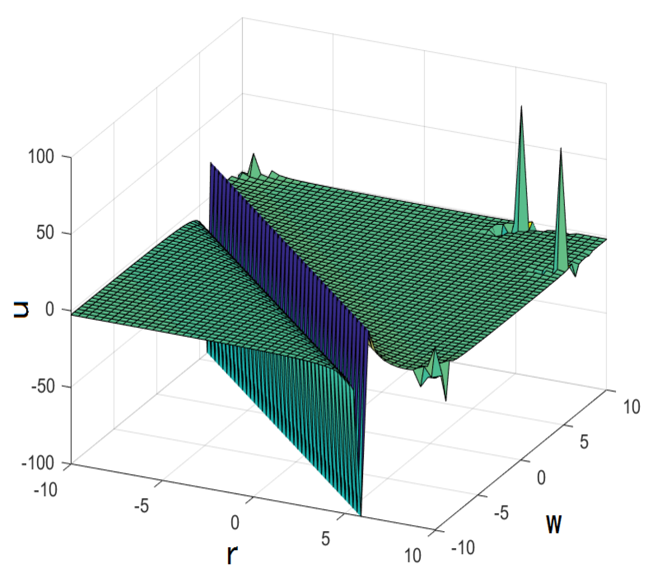
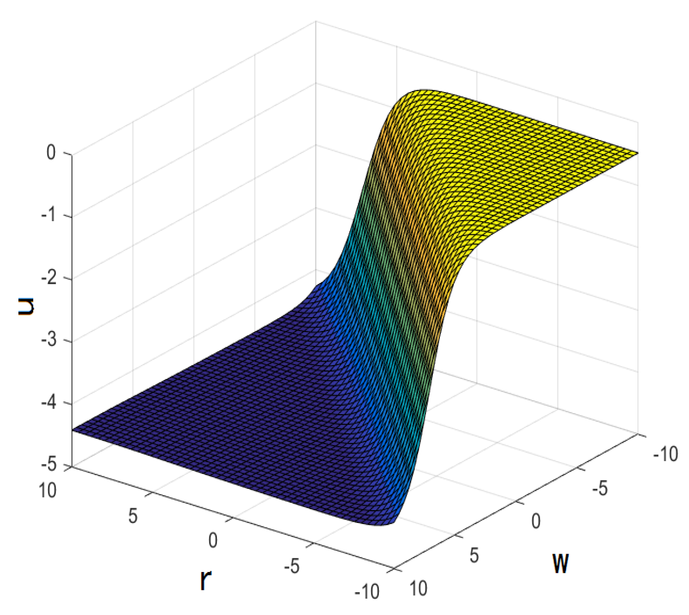
Figure 1. Hyperbolic function $u_{1,1}(\xi )$ as $a=1, c=1, e=\frac{3}{64}, A=2, B=1,$$C_3=\sqrt{5}, E=1,$$M=1, \omega =5, e_0=\frac{13}{24},$$e_1=\frac{3}{2}, C=1, e_2=\frac{1}{2}, d=-2.$

Figure 1. Hyperbolic function $u_{1,1}(\xi )$ as $a=1, c=1, e=\frac{3}{64}, A=2, B=1,$$C_3=\sqrt{5}, E=1,$$M=1, \omega =5, e_0=\frac{13}{24},$$e_1=\frac{3}{2}, C=1, e_2=\frac{1}{2}, d=-2.$

Figure 2. Hyperbolic function $u_{3, 1}(\xi )$ as $a=1, c=1, e=\frac{133}{4}, A=2, B=4,$$C_3=\sqrt{20}, E=1,$$M=1, \omega =20, e_0=-\frac{11}{6},$$e_{-2}=\frac{25}{2}, C=1, e_2=\frac{1}{2}, d=-2.$

Figure 2. Hyperbolic function $u_{3, 1}(\xi )$ as $a=1, c=1, e=\frac{133}{4}, A=2, B=4,$$C_3=\sqrt{20}, E=1,$$M=1, \omega =20, e_0=-\frac{11}{6},$$e_{-2}=\frac{25}{2}, C=1, e_2=\frac{1}{2}, d=-2.$

Figure 3. Hyperbolic function $u_{3, 4}(\xi )$ as $a=1, c=1, e=\frac{5}{4}, A=2, B=0,$$C_3=2, E=1, M=1,$$\Delta =1, e_0=-\frac{1}{2},$$e_{-2}=\frac{1}{2}, C=1, e_2=\frac{1}{2}, d=0.$

Figure 3. Hyperbolic function $u_{3, 4}(\xi )$ as $a=1, c=1, e=\frac{5}{4}, A=2, B=0,$$C_3=2, E=1, M=1,$$\Delta =1, e_0=-\frac{1}{2},$$e_{-2}=\frac{1}{2}, C=1, e_2=\frac{1}{2}, d=0.$

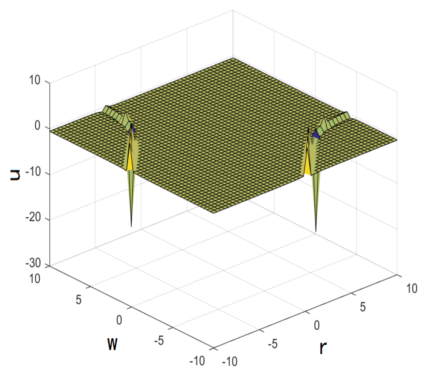
When the exact solution has the form of hyperbolic function, such as $u_{1,1},u_{1,4}$, $u_{2,1}$,$u_{2,4}$, $u_{3,1}$ and $u_{3,4}$. If the solution does not contain the negative power term of $(d+H(\xi ))$, such as $u_{1,1}$ and $u_{1,4}$, it can be inferred from the properties of the hyperbolic tangent function that the image of the solution is smooth. If the solution contains negative power terms of $(d+H(\xi ))$, when the denominator of the solution gradually approaches zero by $\xi$, the image of the solution for $u_{2,1},u_{2,4}$,$u_{3,1}$ and $u_{3,4}$ may reflect sharp points. However, there must be sharp points in the image of solutions $u_{3,1}$ and $u_{3,4}$. For $u_{3,4}$, due to the condition of the auxiliary equation solution $B=-2dM=0,$ and $\Delta >0$, but $M\ne 0,$$d=0$. In this case, the denominator of the negative power term of $(d+H(\xi ))$ is $\frac{\sqrt{\Delta }}{M}tanh(\frac{\sqrt{\Delta }}{A}\xi +C_3)$$\frac{\sqrt{\Delta }}{M}tanh(\frac{\sqrt{\Delta }}{2A}\xi +C_3)$, and $\xi$ can always obtain the value $-\frac{A{C}_3}{\sqrt{\Delta }}$$-\frac{2A{C}_3}{\sqrt{\Delta }}$, so the blow-up phenomenon cannot be avoided and rogue waves will appear in actual phenomena.

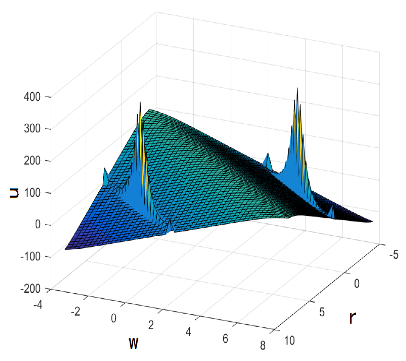
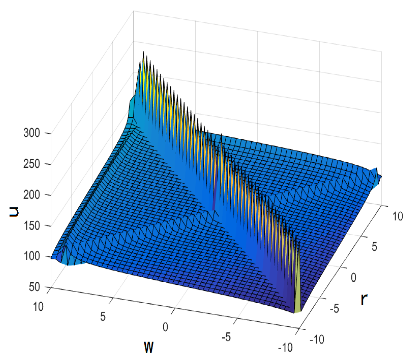
Figure 4. Trigonometric function $u_{1,5}(\xi )$ as $a=1, c=1, A=2,$$B=0, E=-1, M=1,$$\Delta =-1,$$C=1, e_0=\frac{13}{6},$$e_1=2, e_2=\frac{1}{2},$$e=0, C_3=2, d=-2.$

Figure 4. Trigonometric function $u_{1,5}(\xi )$ as $a=1, c=1, A=2,$$B=0, E=-1, M=1,$$\Delta =-1,$$C=1, e_0=\frac{13}{6},$$e_1=2, e_2=\frac{1}{2},$$e=0, C_3=2, d=-2.$

Figure 5. Trigonometric function $u_{2, 2}(\xi )$ as $a=1, c=1, e=-\frac{1}{16},$$B=1, E=-\frac{3}{4}, M=1,$$\omega =-2, C=1, e_0=\frac{9}{8},$$e_{-1}=\frac{33}{8}, e_{-2}=\frac{121}{32},$$A=2, C_3=\sqrt{2}, d=-2.$

Figure 5. Trigonometric function $u_{2, 2}(\xi )$ as $a=1, c=1, e=-\frac{1}{16},$$B=1, E=-\frac{3}{4}, M=1,$$\omega =-2, C=1, e_0=\frac{9}{8},$$e_{-1}=\frac{33}{8}, e_{-2}=\frac{121}{32},$$A=2, C_3=\sqrt{2}, d=-2.$

Figure 6. Trigonometric function $u_{2,5}(\xi )$ as $a=1, c=1, A=2,$$B=0, E=-1, M=1,$$\Delta =-1, C=1, e_0=\frac{13}{6},$$e_{-2}=\frac{25}{2}, e_{-1}=10,$$e=0, C_3=2, d=-2.$

Figure 6. Trigonometric function $u_{2,5}(\xi )$ as $a=1, c=1, A=2,$$B=0, E=-1, M=1,$$\Delta =-1, C=1, e_0=\frac{13}{6},$$e_{-2}=\frac{25}{2}, e_{-1}=10,$$e=0, C_3=2, d=-2.$

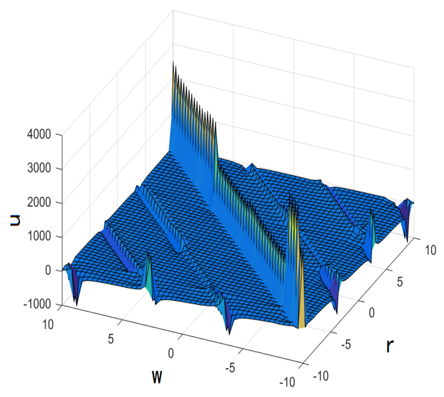
When the exact solution has the form of trigonometric function, such as $u_{1,2}$,$u_{1,5}$,$u_{2,2}$, $u_{2,5}$,$u_{3,2}$ and $u_{3,5}$, from the properties of the tangent function, we deduce that whether the solution contains negative power terms of $(d+H(\xi ))$, the image of the solution will have segmented periodic spikes.

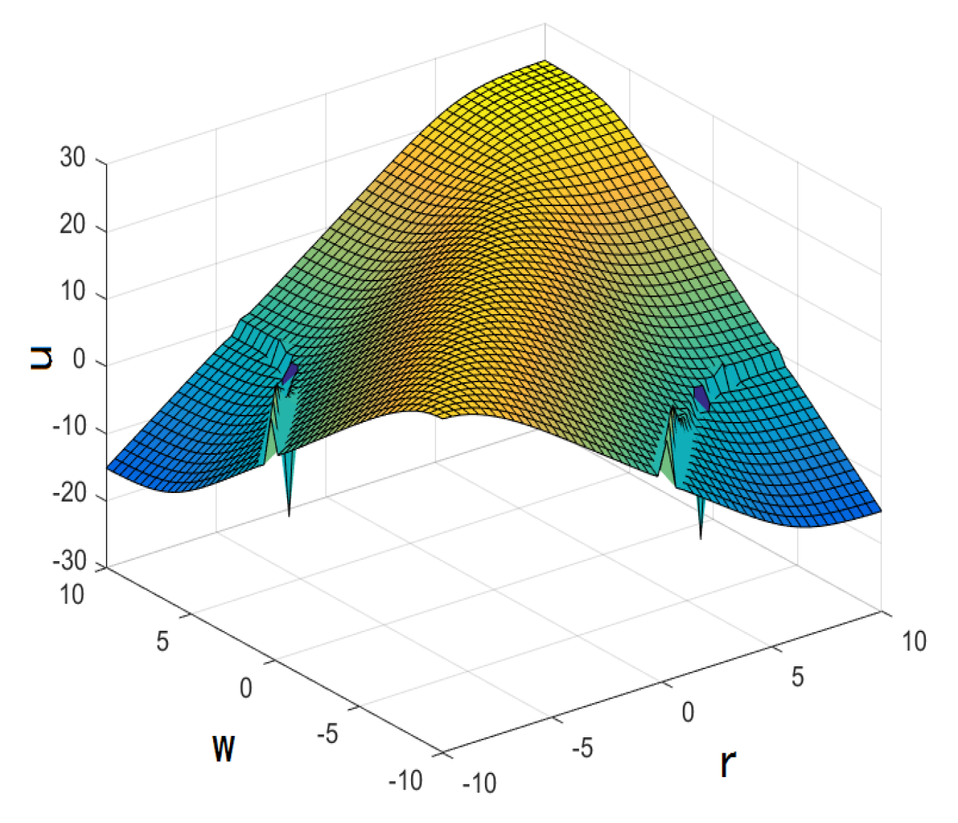
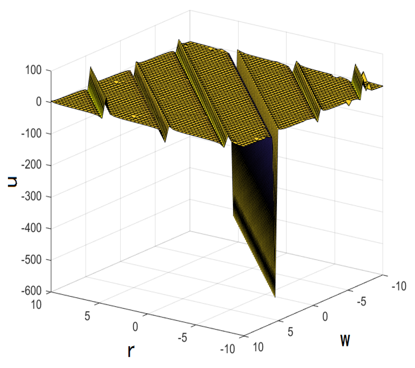
Figure 7. Rational function $u_{1,3}(\xi )$ as $a=1, c=1, e=-\frac{1}{12},$$B=2, E=1, M=-1,$$\omega =0,$$C=2, e_0=\frac{11}{6},$$e_1=-4, e_2=2, A=1,$$C_3=1, d=2.$

Figure 7. Rational function $u_{1,3}(\xi )$ as $a=1, c=1, e=-\frac{1}{12},$$B=2, E=1, M=-1,$$\omega =0,$$C=2, e_0=\frac{11}{6},$$e_1=-4, e_2=2, A=1,$$C_3=1, d=2.$

Figure 8. Rational function $u_{2,3}(\xi )$ as $a=1, c=1, e=-\frac{1}{12},$$B=2, E=1, M=-1,$$\omega =0,$$C=2, e_{-1}=-4,$$A=1, e_{-2}=2, e_0=\frac{11}{6},$$C_3=2, d=2.$

Figure 8. Rational function $u_{2,3}(\xi )$ as $a=1, c=1, e=-\frac{1}{12},$$B=2, E=1, M=-1,$$\omega =0,$$C=2, e_{-1}=-4,$$A=1, e_{-2}=2, e_0=\frac{11}{6},$$C_3=2, d=2.$

Figure 9. Rational function $u_{3,3}(\xi )$$a=1, c=1, e=-\frac{1}{12},$$B=4, E=4, M=-1,$$\omega =0, C=2,$$e_0=-\frac{1}{6},$$A=1, e_2=2, e_{-2}=0,$$C_3=2, d=2.$

Figure 9. Rational function $u_{3,3}(\xi )$$a=1, c=1, e=-\frac{1}{12},$$B=4, E=4, M=-1,$$\omega =0, C=2,$$e_0=-\frac{1}{6},$$A=1, e_2=2, e_{-2}=0,$$C_3=2, d=2.$

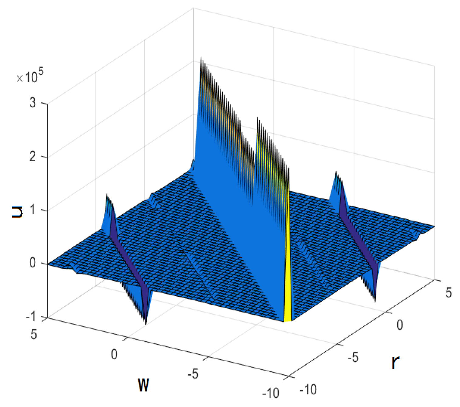
When the exact solution has the form of rational function, such as $u_{1,3},u_{2,3}$ and $u_{3,3}$, since there is always a rational function of $\xi$ in the denominator, there will be sharp points in the image of the solution.

2.4. Numerical Simulation of Solutions under the Same Situation

Now, we discuss the influence of d on the structure and properties of the solution under the same situation.

Figure 10. Hyperbolic function $u_{2,4}(\xi )$ as $d=-2,$$a=1, c=1, A=2, B=0, C_3=2,$$C=1,$$e=0, E=1, M=1, \Delta =1,$$e_0=\frac{3}{2}, e_{-1}=6, e_{-2}=\frac{9}{2}.$

Figure 10. Hyperbolic function $u_{2,4}(\xi )$ as $d=-2,$$a=1, c=1, A=2, B=0, C_3=2,$$C=1,$$e=0, E=1, M=1, \Delta =1,$$e_0=\frac{3}{2}, e_{-1}=6, e_{-2}=\frac{9}{2}.$

Figure 11. Hyperbolic function $u_{2, 4}(\xi )$ as $d=0,$$a=1, c=1, A=2, B=0, C_3=2,$$C=1, e=0,$$E=1, M=1, \Delta =1,$$e_0=-\frac{1}{2}, e_{-1}=0, e_{-2}=\frac{1}{2}.$ .

Figure 11. Hyperbolic function $u_{2, 4}(\xi )$ as $d=0,$$a=1, c=1, A=2, B=0, C_3=2,$$C=1, e=0,$$E=1, M=1, \Delta =1,$$e_0=-\frac{1}{2}, e_{-1}=0, e_{-2}=\frac{1}{2}.$ .

Taking the solution $u_{2,4}$ as an example, which denominator will be $\frac{\sqrt{\Delta }}{M}tanh(\frac{\sqrt{\Delta }}{2A}\xi +C_3)$ when $d=0$, that is a hyperbolic tangent function, but if $\xi$ infinitely approaches $-\frac{A{C}_3}{\sqrt{\Delta }}$, the solution value tends to be infinity, and therefore, blow-up occurs. When $\left|d\right|>\frac{\sqrt{\Delta }}{\left|M\right|}$, the denominator $d+$$\frac{\sqrt{\Delta }}{M}tanh(\frac{\sqrt{\Delta }}{2A}\xi +C_3)$$\ne 0$; then, the function image will be smooth at this time.

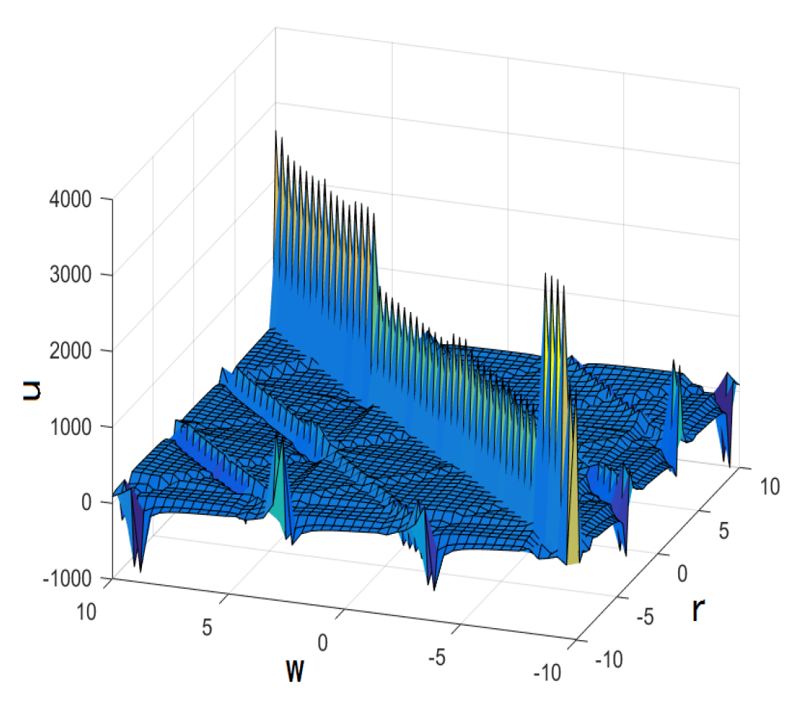
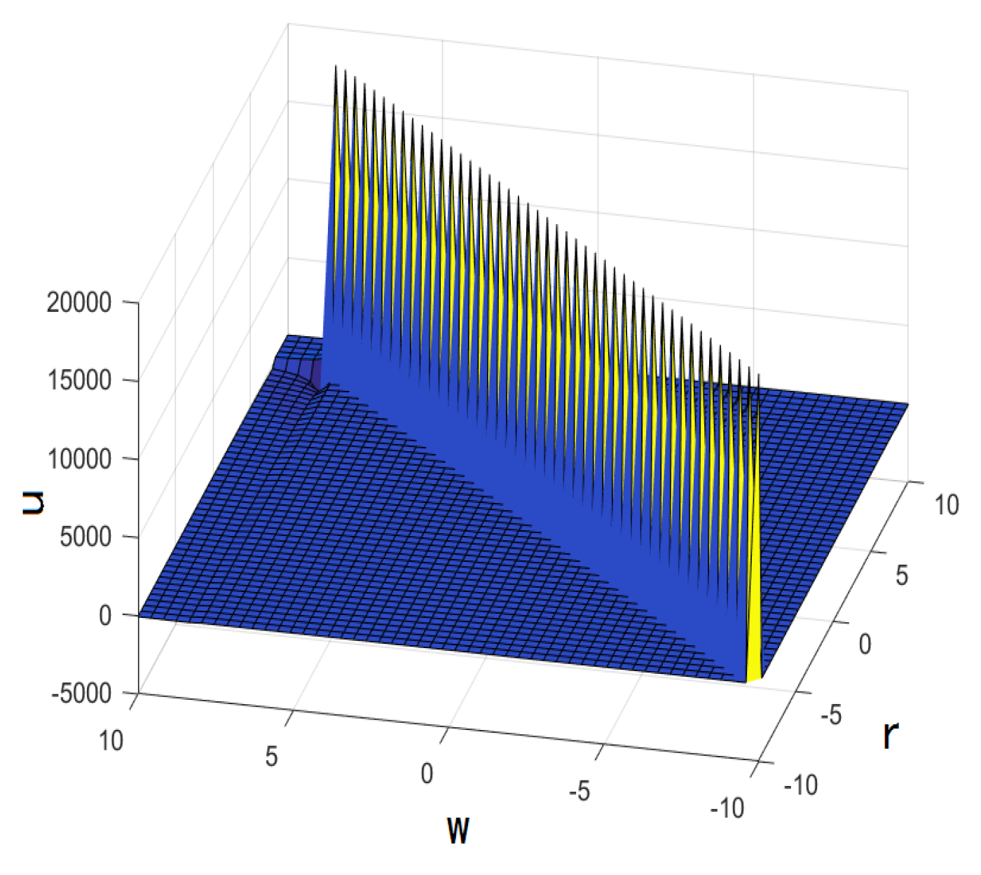
Figure 12. Trigonometric function $u_{3,2}(\xi )$ as $d=-1,$$a=1, c=1, A=2, B=2, E=-2,$$e=\frac{5}{4},$$C=1, M=1, \omega =-4,$$C_3=-2, e_0=\frac{1}{6}, e_2=\frac{1}{2}, e_{-2}=\frac{1}{2}.$

Figure 12. Trigonometric function $u_{3,2}(\xi )$ as $d=-1,$$a=1, c=1, A=2, B=2, E=-2,$$e=\frac{5}{4},$$C=1, M=1, \omega =-4,$$C_3=-2, e_0=\frac{1}{6}, e_2=\frac{1}{2}, e_{-2}=\frac{1}{2}.$

Figure 13. Trigonometric function $u_{3,2}(\xi )$ as $d=0,$$a=1, c=1, A=2, B=0, E=-2,$$e=\frac{21}{4},$$C=1, M=1, \omega =-8,$$C_3=-2, e_0=\frac{1}{2}$,$e_2$$e2$$=\frac{1}{2}, e_{-2}=2.$

Figure 13. Trigonometric function $u_{3,2}(\xi )$ as $d=0,$$a=1, c=1, A=2, B=0, E=-2,$$e=\frac{21}{4},$$C=1, M=1, \omega =-8,$$C_3=-2, e_0=\frac{1}{2}$,$e_2$$e2$$=\frac{1}{2}, e_{-2}=2.$

For $u_{3, 2}$, it is known from the image properties of tangent function that there always exists a $\xi$ so that $\frac{\sqrt{-\omega }}{2M}tan(-\frac{\sqrt{-\omega }}{2A}\xi +C_3)$ is equal to zero no matter what the value d is; then, the solution value is always infinite. These values are periodic, and periodic blow-up will occur.

Comparing those methods mentioned in Refs. [14,15], we add a constant d and negative power terms. Different properties of solutions are obtained by controlling the variable d. The negative power term affects the solution to blow up.

3. Improved Tanh Function Method

3.1. Preliminary

The improved tanh function method makes full use of the generalized Riccati equation

$${\phi }^{\prime }=r+p\phi +q{\phi }^2,$$

(16)

on the basis of the tanh function method, where $r,p$ and q are real constants. For the nonlinear partial differential Equation (4), the steps of the improved tanh function method are as follows.

Step 1

Supposing that Equation (4) has the following form of solution

$$u(x,y,t)=\sum _{i=-N^{\prime }}^{N^{\prime }}{\mu }_i(y,t)\phi {}^i(kx+\eta (y,t)),$$

(17)

where ${\mu }_i(y,t)(i=0,\pm 1,\pm 2,\dots ,\pm N^{\prime })$and $\eta (y,t)$ are differentiable functions, and the value $N^{\prime }$ here is determined by the homogeneous balance principle.

Step 2

Substitute (17) into Equation (4), and repeatedly use Equation (16) to convert the left-hand side of Equation (4) into a polynomial about $\phi (kx+\eta (y,t))$. Equate each coefficient of the same power term to zero, and then obtain the algebraic equations about undetermined functions.

Step 3

Solve the algebraic equations to determine ${\mu }_i(y,t)$ and $\eta (y,t)$, and finally substitute the solution of the generalized Riccati equation into (17).

In the subsequent sections, with the help of the generalized Riccati equation, we will apply the improved tanh function method to solve the non-traveling wave exact solutions of the (2+1)-dimensional Boussinesq equation.

3.2. Expression of Non-Traveling Wave Exact Solution

For the (2+1) dimensional Boussinesq equation

$$u_{tt}-u_{xx}-u_{yy}+3{(u^2)}_{xx}-u_{xxxx}=0,$$

in order to balance the highest derivative term $u_{xxxx}$ and nonlinear term ${(u^2)}_{xx}$, we suppose that Equation (3) has the following form of solution.

$$u(x,y,t)=\frac{a(y,t)}{{\phi }^2}+\frac{b(y,t)}{\phi }+c(y,t)+d(y,t)\phi +e(y,t){\phi }^2,$$

(18)

where $\phi =\phi (kx+\eta (y,t))$, k is a real number but $k\ne 0$, $a(y,t)$, $b(y,t)$, $c(y,t)$, $d(y,t)$, $e(y,t)$ and $\eta (y,t)$ are differentiable functions.

Substituting (18) into Equation (3), and taking $c_0=\frac{k^4{p}^2+8k^{4}qr+k^2-({{\eta }_t}^2-{{\eta }_y}^2)}{6k^2}$, then we obtain the coefficients of $\phi$.

$$\left\{\begin{array}{c}60e{k}^2{q}^2(e-2k^2{q}^2)=0,\hfill \\ 12kq(p(e-2k^2{q}^2)(9e+2k^2{q}^2)+q(d-2k^{2}pq)(6e-2k^2{q}^2))=0,\hfill \\ (e-2k^2{q}^2)(6k^2{p}^2(c-c_0)+4k^4{q}^2{p}^2)+12k^4{q}^4(c-c_0)+e(8k^2{p}^2+16k^{2}qr)\hfill \\ +k^{2}q(d-2k^{2}pq)(21ep-3dp-4k^{2}p{q}^2)=0,\hfill \\ 6k^2(d-2k^{2}pq)[q(20k^2{p}^{2}q+32k^2{q}^{2}r+5dp)+9(p^2+2qr)(e-2k^2{q}^2)]\hfill \\ +6k^2[2rp(e-2k^2{q}^2)(7e+2k^2{q}^2)+2q(beq-k^2{p}^3(e-2k^2{q}^2))]\hfill \\ +2eq({\eta }_{t}t-{\eta }_{y}y)+4q(e_t{\eta }_t-e_y{\eta }_y)=0,\hfill \\ 6k^2[(e-2k^2{q}^2)(3pq(b-2k^{2}pr)+15pr(d-2k^{2}pq)+6e{r}^2)+4k^2{p}^{2}qr-2k^2{p}^4]\hfill \\ +2q(d_t{\eta }_t-d_y{\eta }_y)+4p(e_t{\eta }_t-e_y{\eta }_y)+(e_{tt}-e_{yy})+(2ep+dq)({\eta }_{t}t-{\eta }_{y}y)\hfill \\ +2(d-2k^{2}pq)((p^2+2qr)(d-2k^{2}pq)+k^{2}pq(3p^2+20qr))+6k^2{p}^2{q}^{2}b=0,\hfill \\ 6k^2[r(b-2k^{2}pr)(4k^2{p}^{2}q+6er+3dr)+(e-2k^2{q}^2)(b{p}^2-4k^2{p}^{3}r+2bqr)]\hfill \\ +12b{k}^4{q}^2(p^2+2qr)+(2er+dq)({\eta }_{tt}-{\eta }_{yy})+2p(d_t{\eta }_t-d_y{\eta }_y)\hfill \\ +4r(e_t{\eta }_t-e_y{\eta }_y)+(d_{tt}-d_{yy})=0,\hfill \\ 6k^2[(b-2k^{2}pr)(4k^2{p}^{2}r+b+d{r}^2(d-2k^{2}pq)+ap(a-2k^2{r}^2)(d-2k^{2}pq)]\hfill \\ +6pr{k}^2(e-2k^2{q}^2))+(dr-bq)({\eta }_{tt}-{\eta }_{yy})-2q(b_t{\eta }_t-b_y{\eta }_y)\hfill \\ +2r(d_t{\eta }_t-d_y{\eta }_y)+(c_{tt}-c_{yy})=0,\hfill \\ 6k^2[q(b-2k^{2}pr)(4k^2{p}^{2}r+6aq+3bq)+(a-2k^2{r}^2)(d{r}^2-4k^2{p}^{3}q+2bqr)]\hfill \\ +12d{k}^4{r}^2(p^2+2pr)-(2aq+bp)({\eta }_{tt}-{\eta }_{yy})-2p(b_t{\eta }_t-b_y{\eta }_y)\hfill \\ -4q(a_t{\eta }_t-a_y{\eta }_y)+(b_{tt}-b_{yy})=0,\hfill \\ 6k^2[(a-2k^2{r}^2)(3pr(d-2k^{2}pq)+15pq(b-2k^{2}pr)+6a{q}^2)+4k^2{p}^{2}qr-2k^2{p}^4]\hfill \\ -(2ap+br)({\eta }_{t}t-{\eta }_{y}y)+2r(b_t{\eta }_t-b_y{\eta }_y)-4p(a_t{\eta }_t-a_y{\eta }_y)-(a_{tt}-a_{yy})\hfill \\ +2(b-2k^{2}pr)((p^2+2qr)(b-2k^{2}pr)+k^{2}pr(3p^2+20qr))+6k^2{p}^2{r}^{2}d=0,\hfill \\ 6k^2(b-2k^{2}pr)[r(20k^2{p}^{2}r+32k^2{q}^{2}q+5bp)+9(p^2+2qr)(a-2k^2{r}^2)]\hfill \\ +6k^2[2ap(a-2k^2{r}^2)(7a+2k^2{r}^2)+2r(adr-k^2{p}^3(a-2k^2{r}^2))]\hfill \\ -2ar({\eta }_{tt}-{\eta }_{yy})-4q(a_t{\eta }_t-a_y{\eta }_y)=0,\hfill \\ (a-2k^2{r}^2)(6k^2{p}^2(c-c_0)+a(8k^2{p}^2+16k^{2}qr)+4k^4{r}^2{p}^2)+12k^4{r}^4(c-c_0)\hfill \\ +k^{2}r(b-2k^{2}pr)(21ap-3br-4k^{2}p{r}^2)=0,\hfill \\ 12kr(p(a-2k^2{r}^2)(9a+2k^2{r}^2)+r(b-2k^{2}pr)(6a-2k^2{r}^2))=0,\hfill \\ 60a{k}^2{q}^2(a-2k^2{r}^2)=0.\hfill \end{array}\right.$$

We can obtain the following results by solving those equations with Maple.

Case 1

$$a=0,b=0,d=2k^{2}pq,e=2k^2{q}^2,\eta (y,t)=f_1(y)+f_2(y)t+f_3(t),$$

$$c={\displaystyle \frac{1}{6k^2}}(k^4{p}^2+8k^{4}qr+k^2-({(f_2(y)+f_3^{\prime }(t))}^2-{(f_1^{\prime }(y)+f_2^{\prime }(y)t)}^2)),$$

where $f_1(y),f_2(y)$ and $f_3(t)$ are arbitrary differentiable functions, and ${\eta }_{tt}^2={\eta }_{yy}^2={\eta }_{yt}^2$, while the other two cases are the same.

Case 2

$$a=2k^2{r}^2,b=2k^{2}pr,d=0,e=0,\eta (y,t)=f_1(y)+f_2(y)t+f_3(t),$$

$$c={\displaystyle \frac{1}{6k^2}}(k^4{p}^2+8k^{4}qr+k^2-({(f_2(y)+f_3^{\prime }(t))}^2-{(f_1^{\prime }(y)+f_2^{\prime }(y)t)}^2)).$$

Case 3

$$a=2k^2{r}^2,b=0,d=0,e=0,e=2k^2{q}^2,\eta (y,t)=f_1(y)+f_2(y)t+f_3(t),$$

$$p=0,c={\displaystyle \frac{1}{6k^2}}(8k^{4}qr+k^2-({(f_2(y)+f_3^{\prime }(t))}^2-{(f_1^{\prime }(y)+f_2^{\prime }(y)t)}^2)).$$

For simplicity, we take $M=\frac{\sqrt{p^2-4qr}}{2}$, $N=\frac{\sqrt{4qr-p^2}}{2}$, $\zeta =kx+\eta (y,t)$. Substituting the solutions of the generalized Riccati equation into three cases, we obtain

Case 1

When $p^2-4qr>0$, $pq\ne 0$(or $qr\ne 0$),

$u_1=c-{\displaystyle \frac{k^2}{2}}[p^2-4M^2$tanh${}^2(M\zeta )],$

$u_2=c-{\displaystyle \frac{k^2}{2}}[p^2-4M^2$coth${}^2(M\zeta )],$

$u_3=c-{\displaystyle \frac{k^2}{2}}[p^2-4M^2$(tanh$(2M\zeta )\pm i$sech${(2M\zeta ))}^2],$

$u_4=c-{\displaystyle \frac{k^2}{2}}[p^2-4M^2$(coth$(2M\zeta )\pm$csch${(2M\zeta ))}^2],$

$u_5=c-{\displaystyle \frac{k^2}{2}}[p^2-M^2$(tanh$({\displaystyle \frac{M\zeta }{2}})+$coth$({\displaystyle \frac{M\zeta }{2}}){)}^2],$

$u_6=c-{\displaystyle \frac{k^2{p}^2}{2}}+2k^2{M}^2{\displaystyle \frac{{(\sqrt{A^2+B^2}-A\cosh (2M\zeta ))}^2}{{(A\sinh (2M\zeta )+B)}^2}},$

$u_7=c-{\displaystyle \frac{k^2{p}^2}{2}}+2k^2{M}^2{\displaystyle \frac{{(\sqrt{B^2-A^2}+A\sinh (2M\zeta ))}^2}{{(A\cosh (2M\zeta )+B)}^2}},$

$u_8=c+4k^{2}qr\cosh (M\zeta ){\displaystyle \frac{2qr\cosh (M\zeta )+p(2M\sinh (M\zeta )-p\cosh (M\zeta ))}{{(2M\sinh (M\zeta )-p\cosh (M\zeta ))}^2}},$

$u_9=c+4k^{2}qr\sinh (M\zeta ){\displaystyle \frac{2qr\sinh (M\zeta )+p(2M\cosh (M\zeta )-p\sinh (M\zeta ))}{{(2M\cosh (M\zeta )-p\sinh (M\zeta ))}^2}},$

$u_{10}=c+4k^{2}qr\cosh (2M\zeta ){\displaystyle \frac{(2qr-p^2)\cosh (2M\zeta )+p(2M\sinh (2M\zeta )\pm i2M)}{{(2M\sinh (2M\zeta )-p\cosh (2M\zeta )\pm i2M)}^2}},$

$u_{11}=c+4k^{2}qr\sinh (2M\zeta ){\displaystyle \frac{(2qr-p^2)\sinh (2M\zeta )+p(2M\cosh (2M\zeta )\pm 2M)}{{(2M\cosh (2M\zeta )-p\sinh (2M\zeta )\pm 2M)}^2}},$

$u_{12}=c+8k^{2}qr{\mathsf{\Phi }}_1(\zeta ){\displaystyle \frac{2(2qr-p^2){\mathsf{\Phi }}_1(\zeta )+p(4M{\cosh }^2({\displaystyle \frac{M\zeta }{2}})-2M)}{{(4M{\cosh }^2({\displaystyle \frac{M\zeta }{2}})-2p{\mathsf{\Phi }}_1(\zeta )-2M)}^2}},$

where ${\mathsf{\Phi }}_1(\zeta )=\sinh ({\displaystyle \frac{M\zeta }{2}})\cosh ({\displaystyle \frac{M\zeta }{2}})$, A and B are two non-zero real constants and satisfy $B^2-A^2>0$.

When $p^2-4qr<0$, $pq\ne 0$(or $qr\ne 0$),

$u_{13}=c-{\displaystyle \frac{k^2}{2}}[p^2-4N^2$tan${}^2(N\zeta )],$

$u_{14}=c-{\displaystyle \frac{k^2}{2}}[p^2-4N^2$cot${}^2(N\zeta )],$

$u_{15}=c-{\displaystyle \frac{k^2}{2}}[p^2-4N^2$(tan$(2N\zeta )\pm$sec${(2N\zeta ))}^2],$

$u_{16}=c-{\displaystyle \frac{k^2}{2}}[p^2-4N^2$(cot$(2N\zeta )\pm$csc${(2N\zeta ))}^2],$

$u_{17}=c-{\displaystyle \frac{k^2}{2}}[p^2-N^2$(tan$({\displaystyle \frac{N\zeta }{2}})-$cot$({\displaystyle \frac{N\zeta }{2}}){)}^2],$

$u_{18}=c-{\displaystyle \frac{k^2{p}^2}{2}}+2k^2{N}^2{\displaystyle \frac{{(\sqrt{A^2-B^2}\mp A\cos (2N\zeta ))}^2}{{(A\sin (2N\zeta )+B)}^2}},$

$u_{19}=c-{\displaystyle \frac{k^2{p}^2}{2}}+2k^2{N}^2{\displaystyle \frac{{(\sqrt{A^2-B^2}\mp A\sin (2N\zeta ))}^2}{{(A\cos (2N\zeta )+B)}^2}},$

$u_{20}=c+4k^{2}qr\cos (N\zeta ){\displaystyle \frac{2qr\cos (N\zeta )-p(2N\sin (N\zeta )+p\cos (N\zeta ))}{{(2N\sin (N\zeta )+p\cos (N\zeta ))}^2}},$

$u_{21}=c+4k^{2}qr\sin (N\zeta ){\displaystyle \frac{2qr\sin (N\zeta )+p(2N\cos (N\zeta )-p\sin (N\zeta ))}{{(2N\cos (N\zeta )-p\sin (N\zeta ))}^2}},$

$u_{22}=c+4k^{2}qr\cos (2N\zeta ){\displaystyle \frac{2qr\cos (2N\zeta )-p(2N\sin (2N\zeta )+p\cos (2N\zeta )\pm 2N)}{{(2N\sin (2N\zeta )+p\cos (2N\zeta )\pm 2N)}^2}},$

$u_{23}=c+4k^{2}qr\sin (2N\zeta ){\displaystyle \frac{2qr\sin (2N\zeta )+p(2N\cos (2N\zeta )-p\sin (2N\zeta )\pm 2N)}{{(2N\cos (2N\zeta )-p\sin (2N\zeta )\pm 2N)}^2}},$

$u_{24}=c+8k^{2}qr{\mathsf{\Phi }}_2(\zeta ){\displaystyle \frac{2(2qr-p^2){\mathsf{\Phi }}_2(\zeta )+p(4N{\cos }^2({\displaystyle \frac{N\zeta }{2}})-2N)}{{(4N{\cos }^2({\displaystyle \frac{N\zeta }{2}})-2p{\mathsf{\Phi }}_2(\zeta )-2N)}^2}},$

where ${\mathsf{\Phi }}_2(\zeta )=\sin ({\displaystyle \frac{N\zeta }{2}})\cos ({\displaystyle \frac{N\zeta }{2}}),$ A and B are two non-zero real constants and satisfy $A^2-B^2>0$.

When $r=0$, $pq\ne 0$,

$u_{25}={\displaystyle \frac{1}{6k^2}}(k^4{p}^2+k^2-({(f_2(y)+f_3^{\prime }(t))}^2-{(f_1^{\prime }(y)+f_2^{\prime }(y)t)}^2))$

$-2k^2{p}^2{c}_1{\displaystyle \frac{\cosh (p\zeta )-\sinh (p\zeta )}{{(c_1+\cosh (p\zeta )-\sinh (p\zeta ))}^2}},$

$u_{26}={\displaystyle \frac{1}{6k^2}}(k^4{p}^2+k^2-({(f_2(y)+f_3^{\prime }(t))}^2-{(f_1^{\prime }(y)+f_2^{\prime }(y)t)}^2))$

$-2k^2{p}^2{c}_1{\displaystyle \frac{\cosh (p\zeta )+\sinh (p\zeta )}{{(c_1+\cosh (p\zeta )+\sinh (p\zeta ))}^2}}.$

When $q\ne 0$, $r=p=0$,

$u_{27}={\displaystyle \frac{1}{6k^2}}(k^2-({(f_2(y)+f_3^{\prime }(t))}^2-{(f_1^{\prime }(y)+f_2^{\prime }(y)t)}^2))+{\displaystyle \frac{2k^2{q}^2}{{(c_2+q\zeta )}^2}}.$

Case 2

When $p^2-4qr>0$, $pq\ne 0$(or $qr\ne 0$),

$u_{28}=c-4k^{2}qr{\displaystyle \frac{2Mp\tanh (M\zeta )+p^2-2qr}{{(2M\tanh (M\zeta )+p)}^2}},$

$u_{29}=c-4k^{2}qr{\displaystyle \frac{2Mp\coth M\zeta +p^2-2qr}{{(2M\coth (M\zeta )+p)}^2}},$

$u_{30}=c-4k^{2}qr{\displaystyle \frac{p(2M\tanh (2M\zeta )+p\pm iM\sec \mathrm{h}(2M\zeta ))-2qr}{{(2M\tanh (2M\zeta )+p\pm iM\sec \mathrm{h}(2M\zeta ))}^2}},$

$u_{31}=c-4k^{2}qr{\displaystyle \frac{p(2M\coth (2M\zeta )+p\pm M\csc \mathrm{h}(2M\zeta ))-2qr}{{(2M\coth (2M\zeta )+p\pm M\csc \mathrm{h}(2M\zeta ))}^2}},$

$u_{32}=c-8k^{2}qr{\displaystyle \frac{p(2M\tanh ({\displaystyle \frac{M\zeta }{2}})+2M\coth ({\displaystyle \frac{M\zeta }{2}})+2p)-4qr}{{(2M\tanh ({\displaystyle \frac{M\zeta }{2}})+2M\coth ({\displaystyle \frac{M\zeta }{2}})+2p)}^2}},$

$u_{33}=c-4k^{2}qr{F}_1(\zeta ){\displaystyle \frac{p(2AM\cosh (2M\zeta )+p{F}_1(\zeta )-2M\sqrt{A^2+B^2})-2qr{F}_1(\zeta )}{{(2AM\cosh (2M\zeta )+p{F}_1(\zeta )-2M\sqrt{A^2+B^2})}^2}},$

$u_{34}=c-4k^{2}qr{F}_2(\zeta ){\displaystyle \frac{p(2AM\sinh (2M\zeta )+p{F}_2(\zeta )+2M\sqrt{B^2-A^2})-2qr{F}_2(\zeta )}{{(2AM\sinh (2M\zeta )+p{F}_2(\zeta )+2M\sqrt{B^2-A^2})}^2}},$

$u_{35}=c-{\displaystyle \frac{k^2}{2}}[p^2-M^2{\csc \mathrm{h}}^2({\displaystyle \frac{M\zeta }{2}}){(2\cosh ({\displaystyle \frac{M\zeta }{2}})-\sec \mathrm{h}({\displaystyle \frac{M\zeta }{2}}))}^2],$

where $F_1(\zeta )=A\sinh (2M\zeta )+B$, $F_2(\zeta )=(A\cosh (2M\zeta )+B)$,

A and B are two non-zero real constants and satisfy $B^2-A^2>0$.

When $p^2-4qr<0$, $pq\ne 0$(or $qr\ne 0$),

$u_{36}=c+4k^{2}qr{\displaystyle \frac{2Np\tan (N\zeta )-p^2+2qr}{{(2N\tan (N\zeta )-p)}^2}}$,

$u_{37}=c-4k^{2}qr{\displaystyle \frac{2Np\cot (N\zeta )+p^2-2qr}{{(2N\cot (N\zeta )+p)}^2}}$,

$u_{38}=c+4k^{2}qr{\displaystyle \frac{p(2N\tan (2N\zeta )-p\pm N\sec (2N\zeta ))+2qr}{{(2N\tan (2N\zeta )-p\pm N\sec (2N\zeta ))}^2}}$,

$u_{39}=c-4k^{2}qr{\displaystyle \frac{p(2N\cot (2N\zeta )+p\pm N\csc (2N\zeta ))-2qr}{{(2N\cot (2N\zeta )+p\pm N\csc (2N\zeta ))}^2}}$,

$u_{40}=c+8k^{2}qr{\displaystyle \frac{p(2N\tan ({\displaystyle \frac{N\zeta }{2}})-2N\cot ({\displaystyle \frac{N\zeta }{2}})-2p)+4qr}{{(2N\tan ({\displaystyle \frac{N\zeta }{2}})-2N\cot ({\displaystyle \frac{N\zeta }{2}})-2p)}^2}},$

$u_{41}=c-4k^{2}qr{G}_1(\zeta ){\displaystyle \frac{p(2AN\cos (2N\zeta )+p{G}_1(\zeta )\mp 2N\sqrt{A^2-B^2})-2qr{G}_1(\zeta )}{{(2AN\cos (2N\zeta )+p{G}_1(\zeta )\pm 2N\sqrt{A^2-B^2})}^2}}$,

$u_{42}=c+4k^{2}qr{G}_2(\zeta ){\displaystyle \frac{p(2AN\sin (2N\zeta )-p{G}_2(\zeta )\mp 2N\sqrt{A^2-B^2})+2qr{G}_2(\zeta )}{{(2AN\sin (2N\zeta )-p{G}_2(\zeta )\pm 2N\sqrt{A^2-B^2})}^2}}$,

$u_{43}=c-{\displaystyle \frac{k^2}{2}}[p^2-N^2\csc ({\displaystyle \frac{N\zeta }{2}}){(2\cos ({\displaystyle \frac{N\zeta }{2}})-\sec ({\displaystyle \frac{N\zeta }{2}}))}^2],$

where $G_1(\zeta )=A\sin (2N\zeta )+B$, $G_2(\zeta )=A\cos (2N\zeta )+B$, A and B are two non-zero real constants and satisfy $A^2-B^2>0$.

When $r=0,pq\ne 0$, the solution is independent of x.

When $q\ne 0,r=p=0$, the solution is independent of x.

Case 3 ($p=0$)

When $p^2-4qr>0$, $pq\ne 0$(or $qr\ne 0$),

$u_{44}=c+2k^2{\displaystyle \frac{M^4{\tanh }^4(M\zeta )+q^2{r}^2}{M^2{\tanh }^2(M\zeta )}},$

$u_{45}=c+2k^2{\displaystyle \frac{M^4{\coth }^4(M\zeta )+q^2{r}^2}{M^2{\coth }^2(M\zeta )}},$

$u_{46}=c+2k^2{\displaystyle \frac{M^4{(\tanh (2M\zeta )\pm i\sec \mathrm{h}(2M\zeta ))}^4+q^2{r}^2}{M^2{(\tanh (2M\zeta )\pm i\sec \mathrm{h}(2M\zeta ))}^2}},$

$u_{47}=c+2k^2{\displaystyle \frac{M^4{(\coth (2M\zeta )\pm \csc \mathrm{h}(2M\zeta ))}^4+q^2{r}^2}{M^2{(\coth (2M\zeta )\pm \csc \mathrm{h}(2M\zeta ))}^2}},$

$u_{48}=c+k^2{\displaystyle \frac{M^4{(\tanh ({\displaystyle \frac{M\zeta }{2}})+\coth ({\displaystyle \frac{M\zeta }{2}}))}^4+16q^2{r}^2}{2M^2{(\tanh ({\displaystyle \frac{M\zeta }{2}})+\coth ({\displaystyle \frac{M\zeta }{2}}))}^2}},$

$u_{49}=c+{\displaystyle \frac{k^2{(2M\sqrt{A^2+B^2}-2AM\cosh (2M\zeta ))}^2}{2{(A\sinh (2M\zeta )+B)}^2}}$

$+{\displaystyle \frac{8k^2{r}^2{q}^2{(A\sinh (2M\zeta )+B)}^2}{{(2M\sqrt{A^2+B^2}-2AM\cosh (2M\zeta ))}^2}},$

$u_{50}=c+{\displaystyle \frac{k^2{(2M\sqrt{B^2-A^2}+2AM\sinh (2M\zeta ))}^2}{2{(A\cosh (2M\zeta )+B)}^2}}$

$+{\displaystyle \frac{8k^2{r}^2{q}^2{(A\cosh (2M\zeta )+B)}^2}{{(2M\sqrt{B^2-A^2}+2AM\sinh (2M\zeta ))}^2}},$

$u_{51}=c+2k^2{\displaystyle \frac{M^4{\sinh }^4(M\zeta )+{\cosh }^4(M\zeta )q^2{r}^2}{M^2{\sinh }^2(M\zeta ){\cosh }^2(M\zeta )}},$

$u_{52}=c+2k^2{\displaystyle \frac{M^4{\cosh }^4(M\zeta )+{\sinh }^4(M\zeta )q^2{r}^2}{M^2{\sinh }^2(M\zeta ){\cosh }^2(M\zeta )}},$

$u_{53}=c+{\displaystyle \frac{k^2{(2M\sinh (2M\zeta )\pm i2M)}^2}{2{\cosh }^2(2M\zeta )}}+{\displaystyle \frac{8k^2{q}^2{r}^2{\cosh }^2(2M\zeta )}{{(2M\sinh (2M\zeta )\pm i2M)}^2}},$

$u_{54}=c+{\displaystyle \frac{k^2{(2M\cosh (2M\zeta )\pm 2M)}^2}{2{\sinh }^2(2M\zeta )}}+{\displaystyle \frac{8k^2{q}^2{r}^2{\sinh }^2(2M\zeta )}{{(2M\cosh (2M\zeta )\pm 2M)}^2}},$

$u_{55}=c+{\displaystyle \frac{k^2{(4M{\cosh }^2({\displaystyle \frac{M\zeta }{2}})-2M)}^2}{8{\sinh }^2({\displaystyle \frac{M\zeta }{2}}){\cosh }^2({\displaystyle \frac{M\zeta }{2}})}}+{\displaystyle \frac{32k^{2}qr{\sinh }^2({\displaystyle \frac{M\zeta }{2}}){\cosh }^2({\displaystyle \frac{M\zeta }{2}})}{{(4M{\cosh }^2({\displaystyle \frac{M\zeta }{2}})-2M)}^2}}$,

where A and B are two non-zero real constants and satisfy $B^2-A^2>0$.

When $p^2-4qr<0$, $pq\ne 0$(or $qr\ne 0$),

$u_{56}=c+2k^2{\displaystyle \frac{N^4{\tan }^4(N\zeta )+q^2{r}^2}{N^2\tan (N\zeta )}},$

$u_{57}=c+2k^2{\displaystyle \frac{N^4{\cot }^4(N\zeta )+q^2{r}^2}{N^2\cot (N\zeta )}},$

$u_{58}=c+2k^2{\displaystyle \frac{N^4{(\tan (2N\zeta )\pm \sec (2N\zeta ))}^4+q^2{r}^2}{N^2{(\tan (2N\zeta )\pm \sec (2N\zeta ))}^2}},$

$u_{59}=c+2k^2{\displaystyle \frac{N^4{(\cot (2N\zeta )\pm \csc (2N\zeta ))}^4+q^2{r}^2}{N^2{(\cot (2N\zeta )\pm \csc (2N\zeta ))}^2}},$

$u_{60}=c+k^2{\displaystyle \frac{N^4{(\tan ({\displaystyle \frac{N\zeta }{2}})-\cot ({\displaystyle \frac{N\zeta }{2}}))}^4+16q^2{r}^2}{2N^2{(\tan ({\displaystyle \frac{N\zeta }{2}})-\cot ({\displaystyle \frac{N\zeta }{2}}))}^2}},$

$u_{61}=c+{\displaystyle \frac{2k^2{(\pm N\sqrt{A^2-B^2}-AN\cos (2N\zeta ))}^2}{{(A\sin (2N\zeta )+B)}^2}}+{\displaystyle \frac{2k^2{r}^2{q}^2{(A\sin (2N\zeta )+B)}^2}{{(\pm N\sqrt{A^2-B^2}-AN\cos (2N\zeta ))}^2}},$

$u_{62}=c+{\displaystyle \frac{2k^2{(\pm N\sqrt{A^2-B^2}+AN\sin (2N\zeta ))}^2}{{(A\cos (2N\zeta )+B)}^2}}+{\displaystyle \frac{2k^2{r}^2{q}^2{(A\cos (2N\zeta )+B)}^2}{{(\pm N\sqrt{A^2-B^2}+AN\sin (2N\zeta ))}^2}},$

$u_{63}=c+2k^2{\displaystyle \frac{N^4{\sin }^4(N\zeta )+{\cos }^4(N\zeta )q^2{r}^2}{N^2{\sin }^2(N\zeta ){\cos }^2(N\zeta )}},$

$u_{64}=c+2k^2{\displaystyle \frac{N^4{\cos }^4(N\zeta )+{\sin }^4(N\zeta )q^2{r}^2}{N^2{\sin }^2(N\zeta ){\cos }^2(N\zeta )}},$

$u_{65}=c+{\displaystyle \frac{k^2{(2N\sin (2N\zeta )\pm 2N)}^2}{2{\cos }^2(2N\zeta )}}+{\displaystyle \frac{8k^2{q}^2{r}^2{\cos }^2(2N\zeta )}{{(2N\sin (2N\zeta )\pm 2N)}^2}},$

$u_{66}=c+{\displaystyle \frac{k^2{(2N\cos (2N\zeta )\pm 2N)}^2}{2{\sin }^2(2N\zeta )}}+{\displaystyle \frac{8k^2{q}^2{r}^2{\sin }^2(2N\zeta )}{{(2N\cos (2N\zeta )\pm 2N)}^2}},$

$u_{67}=c+{\displaystyle \frac{k^2{(4N{\cos }^2({\displaystyle \frac{N\zeta }{2}})-2N)}^2}{8{\sin }^2({\displaystyle \frac{N\zeta }{2}}){\cos }^2({\displaystyle \frac{N\zeta }{2}})}}+{\displaystyle \frac{32k^{2}qr{\sin }^2({\displaystyle \frac{N\zeta }{2}}){\cos }^2({\displaystyle \frac{N\zeta }{2}})}{{(4N{\cos }^2({\displaystyle \frac{N\zeta }{2}})-2N)}^2}}$,

where A and B are two non-zero real constants and satisfy $A^2-B^2>0$.

When $r=0$, $pq\ne 0$, but $p=0$, the solution is independent of x.

3.3. Property Analysis of the Solution

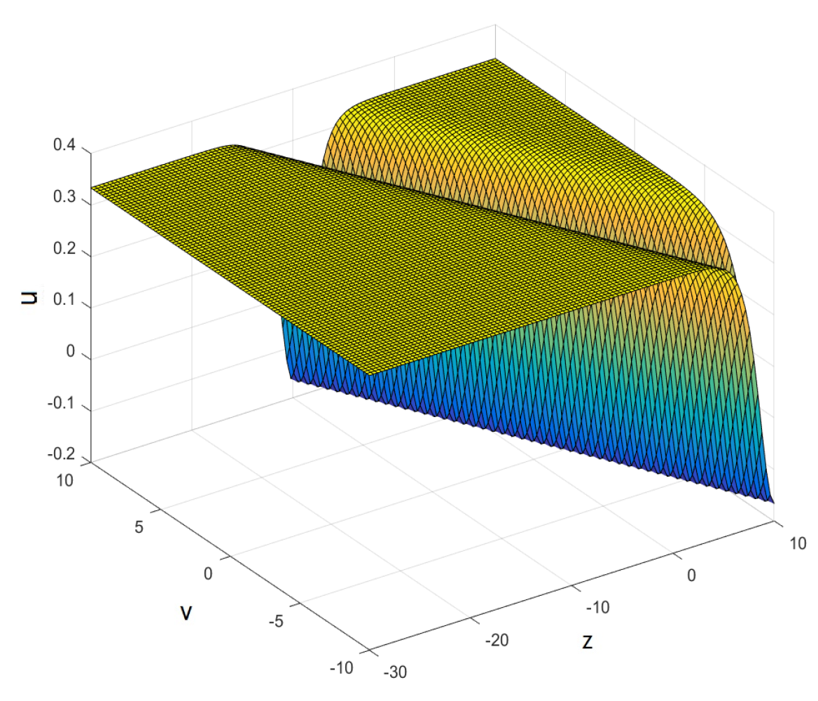
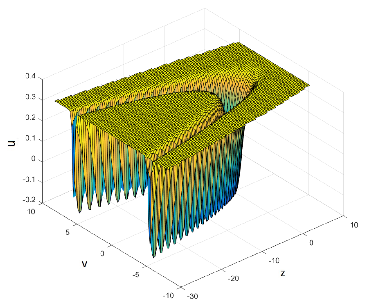
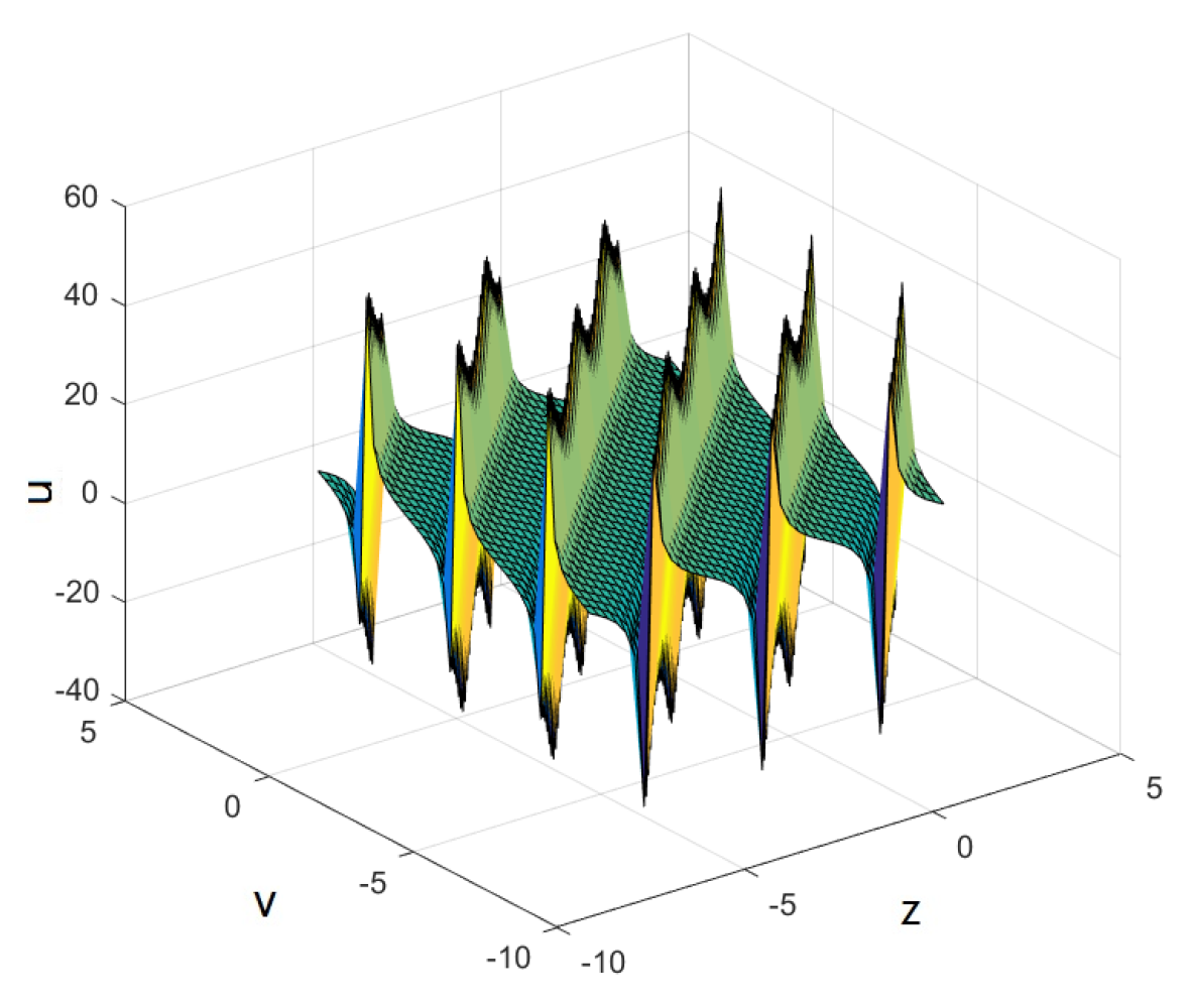
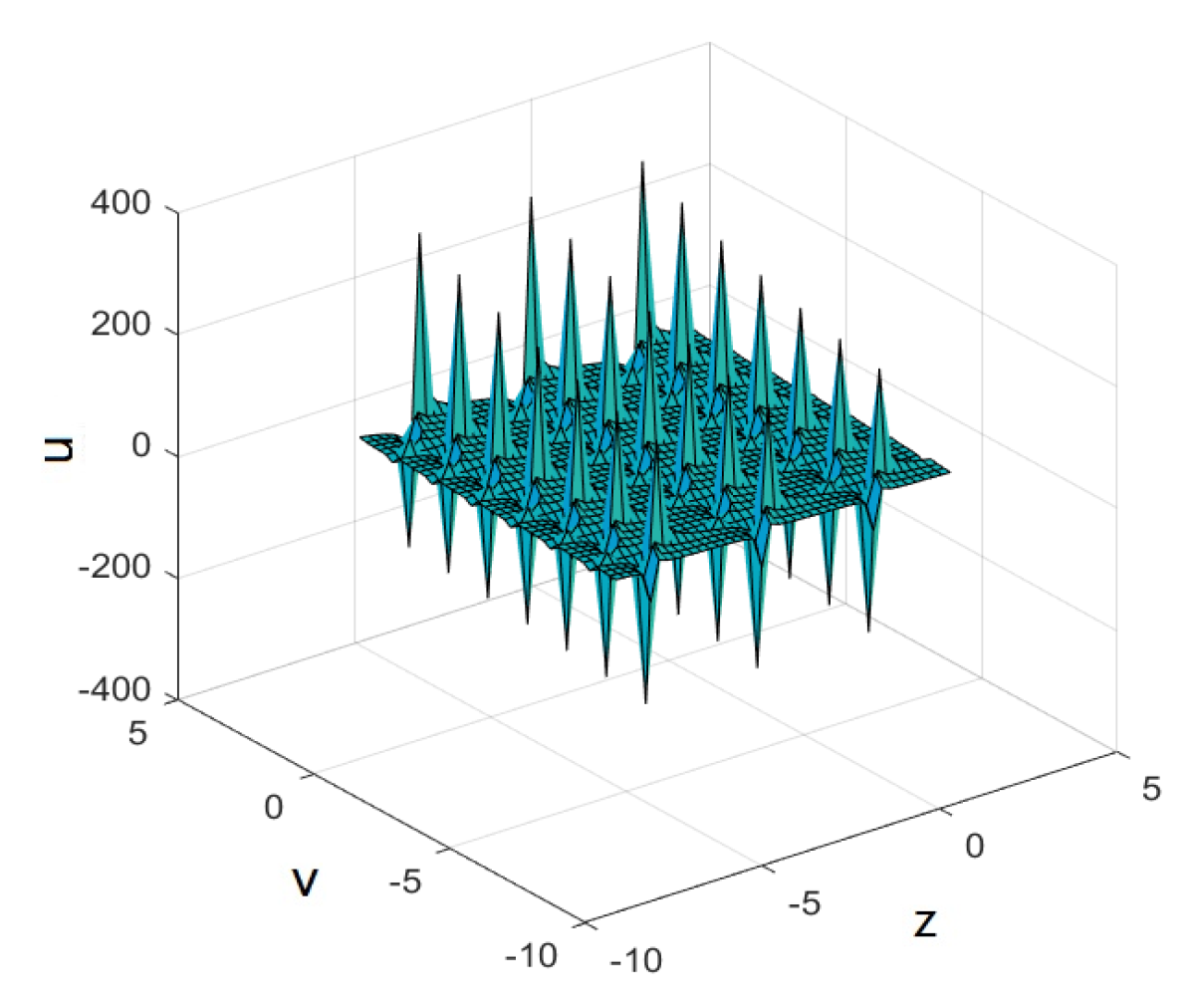
The solutions obtained in this section all include arbitrary differentiable functions $f_1(y),f_2(y)$ and $f_3(t)$, which may give the prediction of physical phenomena with given parameters. According to the expressions of solutions in Case 1, these non-traveling wave solutions can be regarded as kink type, periodic type and singular solitary wave type. Below, we take z$=kx$, $v=y+t$ and give the numerical simulation for the solutions of Case 1.

Figure 14 and Figure 15, respectively, show that when $f_1(y)=y,f_2(y)=0$, $f_3(t)=t$, $\zeta =kx+y+t=$z$+v$, the image of $u_{25}$ shows a linear trajectory in a certain direction; when $f_1(y)=y^2$, $f_2(y)=2y$, $f_3(t)=t^2$, $\zeta =kx+{(y+t)}^2=$z$+v^2$, the image of $u_{25}$ shows a parabolic trajectory in a certain direction. If $c_1=1,p=1$, the denominator ${(1+\cosh (\zeta )-\sinh (\zeta ))}^2$ of $u_{25}$ is always not equal to zero; then, no blow-up occurs, so the images are of all solitary wave. In Figure 16 and Figure 17, $u_{20}$ mainly includes sine functions and cosine functions. If $N=1$, $p=2$, the denominator ${(2\sin (\zeta )+2\cos (\zeta ))}^2$ of $u_{20}$ can be equal to zero, which leads to singularity. However, by comparing $\zeta =$z$+v$ with $\zeta =$z$+v^2$ as an independent variable of trigonometric function, we can intuitively find that the sharps in Figure 17 are multiplied more than those in Figure 16. From the properties of trigonometric function, it can be seen that the images are periodic type. Moreover, each trigonometric function solution in Case 1 is a periodic singular solitary wave solution.

4. Conclusions

In this paper, the exact solutions of the (2+1)-dimension Boussinesq equation are obtained by using the extended $(\frac{G^{\prime }}{G})$ method. For hyperbolic function solutions, such as $u_{3,4}$, the denominator can always obtain zero if $d=0$, and the blow-up phenomenon cannot be avoided. For the trigonometric function solutions, periodic blow-up will occur because of the property and periodicity of the tangent function. For rational function solutions, the solution $u_{3,3}$ contains both positive and negative power terms $(d+H(\xi ))$, the image of solution $u_{3,3}$ is therefore like a superposition of the image of solution $u_{1,3}$ and $u_{2,3}$. Moreover, the rational function of $\xi$ always appears as the denominator, which will lead to blow-up. The formation of rogue waves is reflected by those solutions.

The extended $(\frac{G^{\prime }}{G})$ method is to add a coefficient d to each item in the $(\frac{G^{\prime }}{G})$-expansion, so that the solution becomes the form of $(d+H(\xi ))$. In the fourth hyperbolic function solution of Group 2, it is observed that the smoothness of the image can be controlled by d.

The improved tanh function method is also applied to obtain many non-traveling wave solutions, including kink solutions, periodic solitary wave solutions, and singular solitary wave solutions. Numerical simulation and analysis enables us to better explain the rogue wave phenomenon in natural phenomena. The image of the solution changes greatly under the influence of differentiable function $f_1(y)$, $f_2(y)$ and $f_3(t)$. For example, if $f_1(y)=y^2$, $f_2(y)=2y$, $f_3(t)=t^2$, the image of the solution shows a parabolic trajectory in a certain direction. If we extend these arbitrary differentiable functions, considering trigonometric functions, hyperbolic trigonometric functions, exponential functions, and so on, the equation will have more abundant solutions.

We also find that $u_{1,1}$ and $u_1$ can be expressed as $k_1+k_2{\tanh }^2(k_3\varphi +k_4)$ when $B=-2dM$ and $\varphi (x,y,t)=\phi (kx+\eta (y,t))$ is a linear transformation satisfing ${\eta }_{yy}^2={\eta }_{tt}^2={\eta }_{yt}^2$. Observing the solutions obtained by those two methods, we find that in the extended ($\frac{G^{\prime }}{G}$) method, the $B=-2dM$ is satisfied. In the improved tanh function method, if $\phi (kx+\eta (y,t))$ is a linear transformation of $x,y$ and t, that satisfies the condition ${\eta }_{yy}^2={\eta }_{tt}^2={\eta }_{yt}^2$, which is recorded as $\varphi (x,y,t)$. $u_{1,1}$ and $u_1$ can be simply expressed as $k_1+k_2{\tanh }^2(k_3\varphi +k_4)$, where $k_i(i=1,2,3,4)$ are constants. Moreover, $u_{1,2}$ and $u_{13}$ can be simply expressed as $k_5+k_6{\tan }^2(k_7\varphi +k_8),$ $u_{1,3}$ and $u_{27}$ can be expressed as $k_9+\frac{k_{10}}{{(k_{11}\varphi +k_{12})}^2}$. Here, we only list the solutions of Group 1 and Case 1 obtained by those two methods. These phenomena suggest that there may be some relationships between solutions obtained by different methods for the same equation.

References

- Ghanbari, B. Employing Hirota’s bilinear form to find novel lump waves solutions to an important nonlinear model in fluid mechanics. Results Phys. 2021, 29, 104689. [Google Scholar] [CrossRef]
- Eltayebh, H.; Mesloub, S. Application of Multi-Dimensional of Conformable Sumudu Decomposition Method for Solving Conformable Singular Fractional Coupled Burger’s Equation. Acta Math. Sci. 2021, 41, 1679–1698. [Google Scholar] [CrossRef]
- Wang, Q.; Li, L.Z. Painlevé analysis, Lie symmetry and exact solutions to the generalized time dependent coefficients Gardner equation. J. Shandong Univ. Sci. 2019, 54, 37–44. [Google Scholar]
- Guner, O. New exact solutions for the seventh-order time fractional Sawada-Kotera-Ito equation via various methods. Waves Random Complex Media 2020, 30, 441–457. [Google Scholar] [CrossRef]
- Wang, M.L.; Li, X.Z.; Zhang, J.L. The (G′/G)-expansion method and travelling wave solutions of nonlinear evolution equations in mathematical physics. Phys. Lett. A 2008, 372, 417–423. [Google Scholar] [CrossRef]
- Xie, F.D.; Zhang, Y.; Lü, Z.S. Symbolic computation in non-linear evolution equation: Application to (3+1)-dimensional Kabomtsev-Petviashvili equation. Chaos Solitons Fractals 2005, 24, 257–263. [Google Scholar] [CrossRef]
- Du, B.R.; Zhu, L.S. The application of Boussinesq Equations in the Research on Changes in Wave Induced Set-up and Current after Completion of Engineering. Guangdong Shipbuild. 2012, 31, 47–51. [Google Scholar]
- Song, M.; Shao, S.G. Exact solitary wave solutions of the generalized (2+1)dimensional Boussinesq equation. Appl. Math. Comput. 2010, 7, 3557–3563. [Google Scholar] [CrossRef]
- Zhao, Y.M.; Yang, Y.J.; Jiang, Y. Application of the improved (G′/G)-expansion method to exact solutions for generalized (2+1)-dimensional Boussinesq equation. Pure Appl. Math. 2012, 28, 176–180. [Google Scholar]
- Yang, J.; Feng, Q.J. The Solitary Wave Solutions for Generalized (2+1)-dimensional Boussinesq Equation. Math. Pract. Theory 2017, 47, 230–237. [Google Scholar]
- Zeng, X.; Zhang, H.Q. Backlund transformation and exact solutions for (2 +1)-dimensional Boussinesq equation. Acta Phys. Sin. 2005, 54, 1476–1480. [Google Scholar] [CrossRef]
- Wang, J.M. On Triply Periodic Wave Solutions for (2+1)-Dimensional Boussinesq Equation. Commun. Theor. Phys. 2012, 57, 563–567. [Google Scholar] [CrossRef]
- Liu, Y.K.; Li, B.; An, H.L. General high-order breathers, lumps in the (2+1)-dimensional Boussinesq equation. Nonlinear Dyn. 2018, 92, 2061–2076. [Google Scholar] [CrossRef]
- Wang, W.L.; Feng, S.Q.; Guo, L.N. The Exact Solutions of (2+1)-dimensional Boussinesq Equation. J. Neijiang Norm. Univ. 2011, 26, 21–23. [Google Scholar]
- Li, Z.Q.; Liu, H.Z. Generalized Solution of (2+1)-dimensional Boussinesq Equation. J. Binzhou Univ. 2018, 34, 38–41. [Google Scholar]
- Jiao, X.Y. Truncated series solutions to the (2+1)-dimensional perturbed Boussinesq equation by using the approximate symmetry method. Chin. Phys. B 2018, 27, 127–133. [Google Scholar] [CrossRef]
- Yin, J.Y. Extended expansion method for (G′/G) and new exact solutions of Zakharov equations. Acta Phys. Sin. 2013, 62, 1–5. [Google Scholar]
- Liao, G.J.; Huang, L.W.; Chen, X.; Guo, Y.F. Using extended expansion method to obtain exact solutions of (2+1)-dimensional breaking soliton equation. J. Guangxi Univ. Sci. Technol. 2019, 30, 110–117. [Google Scholar]
- Xu, Y.Q.; Zheng, X.X.; Xin, J. Abundant new non-travelling wave solutions for the (3+1)-dimensional Boiti-Leon-Manna-Pempinelli equation. J. Appl. Anal. Comput. 2021, 11, 2052–2069. [Google Scholar]
- Zhang, S.; Xia, T.C. Symbolic Computation and New Families of Exact Non-travelling Wave Solutions of (2+1)-dimensional Broer-Kaup Equation. Commun. Theor. Phys. 2006, 45, 985–990. [Google Scholar]
- Nather, H.; Abdullah, F.A. New generalized and improved (G′/G)-expansion method for nonlinear evolution equations in mathematical physics. J. Egypt. Math. Soc. 2014, 22, 390–395. [Google Scholar] [CrossRef] [Green Version]
Figure 14.
Linear solitary wave solution as ,
Figure 15.
Parabolic solitary wave solution as ,
Figure 16.
Parabolic and periodic singular wave solution as .
Figure 17.
Publisher’s Note: MDPI stays neutral with regard to jurisdictional claims in published maps and institutional affiliations. |
© 2022 by the authors. Licensee MDPI, Basel, Switzerland. This article is an open access article distributed under the terms and conditions of the Creative Commons Attribution (CC BY) license (https://creativecommons.org/licenses/by/4.0/).
Share and Cite
MDPI and ACS Style
Gao, L.; Guo, C.; Guo, Y.; Li, D. Exact Solutions and Non-Traveling Wave Solutions of the (2+1)-Dimensional Boussinesq Equation. Mathematics 2022, 10, 2522. https://0-doi-org.brum.beds.ac.uk/10.3390/math10142522
AMA Style
Gao L, Guo C, Guo Y, Li D. Exact Solutions and Non-Traveling Wave Solutions of the (2+1)-Dimensional Boussinesq Equation. Mathematics. 2022; 10(14):2522. https://0-doi-org.brum.beds.ac.uk/10.3390/math10142522
Chicago/Turabian StyleGao, Lihui, Chunxiao Guo, Yanfeng Guo, and Donglong Li. 2022. "Exact Solutions and Non-Traveling Wave Solutions of the (2+1)-Dimensional Boussinesq Equation" Mathematics 10, no. 14: 2522. https://0-doi-org.brum.beds.ac.uk/10.3390/math10142522
Note that from the first issue of 2016, this journal uses article numbers instead of page numbers. See further details here.