Output Tracking Control of Random Nonlinear Time-Varying Systems

Abstract

This paper is concerned with the output tracking control problem for random nonlinear systems with time-varying powers. A distinct feature of this paper is that we consider time-varying powers and the second-order moment process simultaneously, which is more practical in real applications than the existing results where only one factor is considered. We propose a new design scheme, which ensures that the fourth moment of the tracking error can be adjusted to be arbitrarily small and all the states of the closed-loop system are bounded in probability. Finally, a numerical simulation is given to demonstrate the feasibility of the control idea.

1. Introduction

Consider the random nonlinear systems (RNSs) with time-varying powers described by

$$\begin{array}{c}\hfill \begin{array}{ccc}{\dot{x}}_j\hfill & =\hfill & {\left[x_{j+1}\right]}^{r_j(t)}+f_j({\overline{x}}_j)+g_j^T({\overline{x}}_j)\zeta (t),j=1,\cdots ,n-1,\hfill \\ {\dot{x}}_n\hfill & =\hfill & {\left[u\right]}^{r_n(t)}+f_n({\overline{x}}_n)+g_n^T({\overline{x}}_n)\zeta (t),\hfill \\ y\hfill & =\hfill & x_1,\hfill \end{array}\end{array}$$

(1)

where ${\overline{x}}_j={(x_1,\cdots ,x_j)}^T\in R^j$, $u\in R$, $y\in R$ are the state, input, and output of the system, respectively. ${\overline{x}}_j(t_0)={(x_{10},\cdots ,x_{j0})}^T$, $t\in [t_0,\infty )$. The time-varying power $r_j(t):R^{+}\to R^{+}$ is a continuous bounded function complying $1\le \underline{r}\le r_j(t)\le \overline{r}$ with two positive constants $\underline{r}$ and $\overline{r}$, and we define ${[·]}^{a(t)}=sign(·){|·|}^{a(t)}$ with $a(t)$ as the time-varying continuous function. The functions $f_j:R^j\to R$ and $g_j:R^j\to R$, $j=1,\cdots ,n$, are smooth, vanishing at the origin. $\zeta (t)\in R^m$ is a standard second-order moment process (SOMP) defined on the complete probability space $(\mathrm{\Omega },\mathcal{F},{\mathcal{F}}_t,\mathcal{P})$ with a filtration ${\mathcal{F}}_t$ complying the general requirements. A given ${\mathcal{C}}^1$ target signal is defined as $y_0(t)\in R$ (${\mathcal{C}}^1$ represents a class of functions whose derivatives are continuous).

When the noise $\zeta (t)$ in system (1) is white noise, system (1) is called stochastic nonlinear systems (SNSs), and there are many results on its control design. Reference [1] explores the adaptive output feedback tracking problems for SNSs with the unknown state, and [2] considers the strict-feedback SNSs with unknown parameters in the drift terms or the diffusion terms. State feedback tracking control of SNSs was studied in [3]. Reference [4] investigates the global output feedback stabilization for SNSs. Reference [5] presents mean-nonovershooting tracking control designs for strict-feedback SNSs. Reference [6] solves the prescribed-time mean-square stabilization and inverse optimality control problems for strict-feedback SNSs by developing a new nonscaling backstepping design scheme. Reference [7] solves the finite-time stabilization problem of stochastic low-order nonlinear systems with time-varying orders and stochastic inverse dynamics. In [8], a new observer design for a class of nonlinear systems with unknown, bounded, time-varying delays was presented. In [9], the authors studied the finite time stability of equilibrium points of the Caputo–Katugampola fractional neural networks with time delays and proved its existence and uniqueness.

The results in [1,2,3,4,5,6,7] is based on $r_j(t)=1$. When $r_j(t)$ is greater than 1, system (1) is understood as high power systems. There are also many studies on higher power systems. Reference [10] investigated the finite-time stabilization of output-constrained systems with stochastic inverse dynamics and high-order and low-order nonlinearities. Reference [11] presented an adaptive state-feedback strategy for state-constrained systems. In [12], the authors were concerned with the problem of robust cooperative output tracking. According to the results in [10,11,12], the orders are required to be constants. However, there are many systems with time-varying powers in practical industrial applications. For example, it is clear that the power of boiler turbine units in [13] is time-varying. In addition, the underactuated mechanical system in [14] is also a time-varying system. The reason is the performance hidden trouble brought by spring hardening. Recently, ref. [15] presented two types of controllers for SNSs with time-varying powers, namely the state feedback controller and optimal controller. Reference [16] studied the adaptive control of systems with time-varying power.

White noise is considered a disturbance in the above results. It is undeniable that white noise has its own unique advantages in theoretical analysis. However, in many engineering systems, SOMP is more reasonable for model disturbances. References [17,18,19] propose two stability theories for this type of system (RNSs with SOMP). Reference [19] considers the stabilization for RNSs. The trajectory tracking of random Lagrange systems disturbed is studied in [20]. Reference [21] discussed the adaptive tracking control for RNSs. Reference [22] investigated the stability of the nonlinear benchmark system in vibrating environments. Reference [23] focused on cooperative control for multiple benchmark systems. References [19,20,21,22,23] focused on tracking problems. There are also some studies on the stability of random systems. For example, stability in the presence of time delay [24], unified stability criteria [25], global asymptotic stability, and stabilization [26]. Nevertheless, there are currently no published results on tracking the control of higher-order RNSs with time-varying powers.

In this paper, we focus on output tracking control for a class of high-order RNSs with time-varying powers. Compared with the available results, the main contributions of this paper are two-fold:

(1)

This paper is the first result on the output tracking topic of high-order RNSs with time-varying powers. To extend the order of the system to the time-varying power domain, a new method is proposed to design the controller to achieve stability analysis. Different from [15]’s method, the time-varying order of the system considered in this paper is not uniform $r(t)$ and we consider different orders, i.e., $r_i(t)\ne r_j(t)$, $i\ne j$.

(2)

Unlike the deterministic systems [16], the systems studied in this paper are perturbed by SOMP. In the controller design, how to reasonably separate the SOMP from the nonlinear functions is a challenging problem. This is completely different from the designs with white noise in [1,2,3,4,5,6,7,8,9,10,11,12,13,14,15].

This paper includes four parts. Section 2 is the control design and analysis. Section 3 illustrates the effectiveness of the control method by a simulation example. Section 4 presents the conclusions.

2. Control Design and Analysis

For system (1), we need the following assumptions.

Assumption 1.

For the target signal $y_0(t)\in R$, we assume that $y_0(t)$ and ${\dot{y}}_0(t)$ satisfy $|y_0|+|{\dot{y}}_0|\le M$, where M is a positive constant.

Assumption 2.

There exist nonnegative smooth functions ${\theta }_i({\overline{x}}_i)$ and ${\varphi }_i({\overline{x}}_i)$, $i=1,\dots ,n$, such that

$$|f_i({\overline{x}}_i)|\le {\theta }_i({\overline{x}}_i),$$

$$|g_i({\overline{x}}_i)|\le {\varphi }_i({\overline{x}}_i).$$

Assumption 3.

$\zeta (t)$ is the ${\mathcal{F}}_t-$ adapted and piecewise continuous process satisfying ${sup}_{t\ge t_0}E{|\zeta (t)|}^2<K$, where $K>0$ is a constant.

Remark 1.

Assumption 3 shows that the random process $\zeta (t)$ is a second-order moment process. As shown in [19,20,21,22,23,24,25,26], this kind of noise characterizes the physical system more reasonably than white noise.

The objective of this paper was to design an output tracking controller for system (1), such that the closed-loop system has a unique solution on $[t_0,\infty )$, all states are bounded in probability and the tracking error’s 4th moment can be tuned arbitrarily small.

2.1. Controller Design

For system (1), we adopted the coordinate changes

$$\begin{array}{ccc}\hfill {\eta }_i& =& x_i-x_i^{\ast },\hfill \end{array}$$

(2)

where $x_i^{\ast }$, $i=2,\cdots ,n$, are intermediate controllers, the specific form of which is given in the following section. In particular, $x_1^{\ast }=y_0$. Then we have

$$\begin{array}{ccc}\hfill {\dot{\eta }}_i& =& {\left[x_{i+1}\right]}^{r_i(t)}+f_i({\overline{x}}_i)+g_i^T({\overline{x}}_i)\zeta (t)-\sum _{k=1}^{i-1}\frac{\partial x_i^{\ast }}{\partial x_k}({\left[x_{k+1}\right]}^{r_k(t)}+f_k({\overline{x}}_k)\hfill \\ & & +g_k^T({\overline{x}}_k)\zeta (t))-\frac{\partial x_i^{\ast }}{\partial y_0}{\dot{y}}_0,\hfill \end{array}$$

(3)

where $x_{n+1}=u$.

Next, we give the design process of the system (1).

Step 1. We first designed $x_2^{\ast }$.

According to (2) and (3), we obtain

$$\begin{array}{c}\hfill {\eta }_1=x_1-x_1^{\ast }=x_1-y_0,\end{array}$$

(4)

and

$$\begin{array}{ccc}\hfill {\dot{\eta }}_1& =& {\left[x_2\right]}^{r_1(t)}+f_1+g_1^T\zeta -{\dot{y}}_0.\hfill \end{array}$$

(5)

Meanwhile, we choose the Lyapunov function $V_1=\frac{1}{4}{\eta }_1^4$. From (5) and Assumptions 1 and 2, we have

$$\begin{array}{c}\hfill \begin{array}{ccc}\dot{V_1}\hfill & =\hfill & {\eta }_1^3{\dot{\eta }}_1\hfill \\ \hfill & =\hfill & {\eta }_1^3({\left[x_2\right]}^{r_1(t)}+f_1+g_1^T\zeta -{\dot{y}}_0)\hfill \\ \hfill & \le \hfill & {\eta }_1^3({\left[x_2\right]}^{r_1(t)}+f_1+g_1^T\zeta +M).\hfill \end{array}\end{array}$$

(6)

By Assumption 2 and Lemma 2.2 in [27], we obtain

$$\begin{array}{c}\hfill {\eta }_1^3(f_1+M)\le {\eta }_1^3({\theta }_1({\overline{x}}_1)+M)\le {\beta }_{11}({\overline{x}}_1){|{\eta }_1|}^{\overline{r}+3}+{ϵ}_{11},\end{array}$$

(7)

where ${\beta }_{11}({\overline{x}}_1)=\frac{3}{\underline{r}+3}{(\frac{\overline{r}}{{ϵ}_{11}(3+\underline{r})})}^{\frac{\overline{r}}{3}}{({\theta }_1({\overline{x}}_1)+M)}^{\frac{\overline{r}+3}{3}}$, and ${ϵ}_{11}$ is a positive constant.

By Assumption 2 and Lemma 2.2 in [27], we have

$$\begin{array}{c}\hfill \begin{array}{ccc}{\eta }_1^3{g}_1^T\zeta \hfill & \le \hfill & {\eta }_1^3{\varphi }_1({\overline{x}}_1)\zeta \hfill \\ \hfill & \le \hfill & {ϵ}_{121}{\eta }_1^6{\varphi }_1^2({\overline{x}}_1)+\frac{1}{4{ϵ}_{121}}{|\zeta |}^2\hfill \\ \hfill & \le \hfill & {\beta }_{12}({\overline{x}}_1)|{\eta }_1{|}^{\overline{r}+3}+\frac{1}{4{ϵ}_{121}}{|\zeta |}^2+{ϵ}_{122},\hfill \end{array}\end{array}$$

(8)

where ${ϵ}_{121}$ and ${ϵ}_{122}$ are positive constants, ${\beta }_{12}({\overline{x}}_1)=\frac{3}{\underline{r}+3}{(\frac{{ϵ}_{122}\overline{r}}{(3+\underline{r})})}^{\frac{\overline{r}}{3}}{ϵ}_{121}^{\frac{\overline{r}+3}{3}}$ ${\eta }_1^{\overline{r}+3}{({\varphi }_1({\overline{x}}_1))}^{\frac{2\overline{r}+6}{3}}$.

Importing (7) and (8) into (6) can cause

$$\begin{array}{ccc}\hfill \dot{V_1}& \le & {\eta }_1^3{\left[x_2\right]}^{r_1(t)}+{\beta }_{11}({\overline{x}}_1)|{\eta }_1{|}^{\overline{r}+3}+{ϵ}_{11}+{\beta }_{12}({\overline{x}}_1)|{\eta }_1{|}^{\overline{r}+3}+\frac{1}{4{ϵ}_{121}}{|\zeta |}^2+{ϵ}_{122}\hfill \\ & =& {\eta }_1^3({\left[x_2\right]}^{r_1(t)}-{\left[x_2^{\ast }\right]}^{r_1(t)})+{\eta }_1^3{\left[x_2^{\ast }\right]}^{r_1(t)}+{\beta }_1({\overline{x}}_1)|{\eta }_1{|}^{\overline{r}+3}+{\delta }_{11}+{\delta }_{12}{|\zeta |}^2,\hfill \end{array}$$

(9)

where ${\beta }_1({\overline{x}}_1)={\beta }_{11}({\overline{x}}_1)+{\beta }_{12}({\overline{x}}_1)$, ${\delta }_{11}={ϵ}_{11}+{ϵ}_{122}$, ${\delta }_{12}=\frac{1}{4{ϵ}_{121}}$.

So, we choose

$$\begin{array}{c}\hfill x_2^{\ast }=-{\alpha }_1({\overline{x}}_1)({\eta }_1+{\left[{\eta }_1\right]}^{\overline{r}})=-{(c_1+{\beta }_1({\overline{x}}_1))}^{\frac{1}{\underline{r}}}({\eta }_1+{\left[{\eta }_1\right]}^{\overline{r}}),\end{array}$$

(10)

such that

$$\begin{array}{c}\hfill {\eta }_1^3{\left[x_2^{\ast }\right]}^{r_1(t)}=-{\alpha }_1^{r_1(t)}({\overline{x}}_1){({\eta }_1+{\left[{\eta }_1\right]}^{\overline{r}})}^{r_1(t)}{\eta }_1^3,\end{array}$$

(11)

where $c_1\ge 1$ is a free parameter, ${\alpha }_1(x_1)\ge 1$ is a smooth function uncorrelated of $r_1(t)$.

By Lemma 2.3 in [27], we have

$$\begin{array}{c}\hfill {\eta }_1^3{({\eta }_1+{\left[{\eta }_1\right]}^{\overline{r}})}^{r_1(t)}\ge |{\eta }_1{|}^{r_1(t)+3}+{|{\eta }_1|}^{\overline{r}{r}_1(t)+3}.\end{array}$$

(12)

Thus, we have

$$\begin{array}{c}\hfill {\eta }_1^3{\left[x_2^{\ast }\right]}^{r_1(t)}\le -(c_1+{\beta }_1({\overline{x}}_1))(|{\eta }_1{|}^{r_1(t)+3}+|{\eta }_1{|}^{\overline{r}{r}_1(t)+3}),\end{array}$$

(13)

and by Lemma 3 in [16], we obtain

$$\begin{array}{c}\hfill |{\eta }_1{|}^{\overline{r}+3}\le |{\eta }_1{|}^{r_1(t)+3}+{|{\eta }_1|}^{\overline{r}{r}_1(t)+3}.\end{array}$$

(14)

From (9) and (10), we have

$$\begin{array}{ccc}\hfill \dot{V_1}& \le & -c_1|{\eta }_1{|}^{\overline{r}+3}+{\eta }_1^3({\left[x_2\right]}^{r_1(t)}-{\left[x_2^{\ast }\right]}^{r_1(t)})+{\delta }_{11}+{\delta }_{12}{|\zeta |}^2.\hfill \end{array}$$

(15)

Step 2. We then design $x_3^{\ast }$.

From (2), we have

$$\begin{array}{ccc}\hfill {\dot{\eta }}_2& =& {\left[x_3\right]}^{r_2(t)}+\left(f_2({\overline{x}}_2)-\frac{\partial x_2^{\ast }}{\partial x_1}({\left[x_2\right]}^{r_1(t)}+f_1({\overline{x}}_1))\right)-\frac{\partial x_2^{\ast }}{\partial y_0}{\dot{y}}_0\hfill \\ & & +g_2^T({\overline{x}}_2)\zeta -\frac{\partial x_2^{\ast }}{\partial x_1}{g}_1^T\zeta .\hfill \end{array}$$

(16)

Choosing $V_2=V_1+\frac{1}{4}{\eta }_2^4$, by (15) and (16), we obtain

$$\begin{array}{c}\hfill \begin{array}{ccc}{\dot{V}}_2\hfill & \le \hfill & -c_1|{\eta }_1{|}^{\overline{r}+3}+{\eta }_1^3({\left[x_2\right]}^{r_1(t)}-{\left[x_2^{\ast }\right]}^{r_1(t)})+{\delta }_{11}+{\delta }_{12}{|\zeta |}^2\hfill \\ \hfill & \hfill & +{\eta }_2^3({\left[x_3\right]}^{r_2(t)}+\left(f_2({\overline{x}}_2)-\frac{\partial x_2^{\ast }}{\partial x_1}({\left[x_2\right]}^{r_1(t)}+f_1({\overline{x}}_1))\right)-\frac{\partial x_2^{\ast }}{\partial y_0}\dot{y_0}\hfill \\ \hfill & \hfill & +g_2^T({\overline{x}}_2)\zeta -\frac{\partial x_2^{\ast }}{\partial x_1}{g}_1^T\zeta ).\hfill \end{array}\end{array}$$

(17)

According to Lemma 2.1 in [27], we obtain

$$\begin{array}{c}\hfill \begin{array}{ccc}{\eta }_1^3({\left[x_2\right]}^{r_1(t)}-{\left[x_2^{\ast }\right]}^{r_1(t)})\hfill & \le \hfill & \overline{r}(2^{\overline{r}-2}+2)(|{\eta }_1{|}^3|{\eta }_2{|}^{r_1(t)}+{\alpha }_1^{\overline{r}-1}|{\eta }_1{|}^{r_1(t)+2}|{\eta }_2|)\hfill \\ \hfill & \le \hfill & \overline{r}(2^{\overline{r}-2}+2)|{\eta }_1{|}^3(|{\eta }_2{|}^{\overline{r}}+|{\eta }_2|)+\overline{r}(2^{\overline{r}-2}+2){\alpha }_1^{\overline{r}-1}\hfill \\ \hfill & \hfill & ·(|{\eta }_1{|}^{\overline{r}+2}+|{\eta }_1{|}^3)|{\eta }_2|.\hfill \end{array}\end{array}$$

(18)

From Lemma 2.2 in [27], we have

$$\begin{array}{c}\hfill \begin{array}{ccc}\overline{r}(2^{\overline{r}-2}+2)({\alpha }_1^{\overline{r}-1}+1)|{\eta }_1{|}^3|{\eta }_2|\hfill & \le \hfill & {ϵ}_{21}+{\beta }_{211}(x_1){|{\eta }_2|}^{\overline{r}+3},\hfill \\ \overline{r}(2^{\overline{r}-2}+2){\alpha }_1^{\overline{r}-1}|{\eta }_1{|}^{\overline{r}+2}|{\eta }_2|\hfill & \le \hfill & \frac{1}{2}|{\eta }_1{|}^{\overline{r}+3}+{\beta }_{212}(x_1){|{\eta }_2|}^{\overline{r}+3},\hfill \\ \overline{r}(2^{\overline{r}-2}+2)|{\eta }_1{|}^3{|{\eta }_2|}^{\overline{r}}\hfill & \le \hfill & \frac{1}{2}|{\eta }_1{|}^{\overline{r}+3}+{\beta }_{213}{|{\eta }_2|}^{\overline{r}+3},\hfill \end{array}\end{array}$$

(19)

where

$$\begin{array}{ccc}\hfill {\beta }_{211}(x_1)& =& \frac{1}{\underline{r}+3}{\left(\frac{\overline{r}+2}{(\underline{r}+3){ϵ}_{211}}\right)}^{\overline{r}+2}{\left(\overline{r}(2^{\overline{r}-2}+2){({(x_1+1)}^2+1)}^{\frac{3}{2}}({\alpha }_1^{\overline{r}-1}+1)\right)}^{\overline{r}+3},\hfill \\ \hfill {\beta }_{212}(x_1)& =& \frac{1}{\underline{r}+3}{\left(\overline{r}(2^{\overline{r}-2}+2){\alpha }_1^{\overline{r}-1}\right)}^{\overline{r}+3}{\left(\frac{\underline{r}+3}{2\overline{r}+4}\right)}^{-(\overline{r}+2)},\hfill \\ \hfill {\beta }_{213}& =& \frac{\overline{r}}{\underline{r}+3}{\left(\frac{6}{\underline{r}+3}\right)}^{\frac{\overline{r}}{3}}{\left(\overline{r}(2^{\overline{r}-2}+2)\right)}^{\frac{\overline{r}+3}{\underline{r}}}.\hfill \end{array}$$

Substituting (19) into (18), we have

$$\begin{array}{c}\hfill {\eta }_1^3({\left[x_2\right]}^{r_1(t)}-{\left[x_2^{\ast }\right]}^{r_1(t)})\le |{\eta }_1{|}^{\overline{r}+3}+{\beta }_{21}(x_1){|{\eta }_2|}^{\overline{r}+3}+{ϵ}_{21},\end{array}$$

(20)

where ${\beta }_{21}(x_1)={\beta }_{211}(x_1)+{\beta }_{212}(x_1)+{\beta }_{213}\ge 0$ is uncorrelated of $r_1(t)$, ${ϵ}_{21}$ is positive constant.

Estimate the sixth term of (17) as

$$\begin{array}{c}\hfill \begin{array}{ccc}\hfill & \hfill & {\eta }_2^3\left(f_2({\overline{x}}_2)-\frac{\partial x_2^{\ast }}{\partial x_1}({\left[x_2\right]}^{r_1(t)}+f_1({\overline{x}}_1))-\frac{\partial x_2^{\ast }}{\partial y_0}{\dot{y}}_0\right)\hfill \\ \hfill & \le \hfill & {\eta }_2^3\left[{\theta }_2({\overline{x}}_2)+\frac{\partial x_2^{\ast }}{\partial x_1}{(x_2+1)}^{\frac{\overline{r}}{2}}+{\theta }_1(x_1))+\frac{\partial x_2^{\ast }}{\partial y_0}M\right]\hfill \\ \hfill & \le \hfill & {\beta }_{22}(x_1){|{\eta }_2|}^{\overline{r}+3}+{ϵ}_{22},\hfill \end{array}\end{array}$$

(21)

where

$$\begin{array}{ccc}\hfill {\beta }_{22}(x_1)& =& \frac{3}{\overline{r}+3}{\left(\frac{\overline{r}}{{ϵ}_{22}(\underline{r}+3)}\right)}^{\frac{\overline{r}}{3}}{\left[{\theta }_2({\overline{x}}_2)+\frac{\partial x_2^{\ast }}{\partial x_1}{(x_2+1)}^{\frac{\overline{r}}{2}}+{\theta }_1(x_1))+\frac{\partial x_2^{\ast }}{\partial y_0}M\right]}^{\frac{\overline{r}+3}{3}},\hfill \end{array}$$

with ${ϵ}_{22}$ being a positive constant.

For the term in (17) involving the SOMP, we have

$$\begin{array}{ccc}\hfill {\eta }_2^3\left(g_2^T({\overline{x}}_2)\zeta -\frac{\partial x_2^{\ast }}{\partial x_1}{g}_1^T({\overline{x}}_1)\zeta \right)& \le & {ϵ}_{231}{\eta }_2^6{\left({\varphi }_2({\overline{x}}_2)+\frac{\partial x_2^{\ast }}{\partial x_1}{\varphi }_1^T({\overline{x}}_1)\right)}^2+\frac{1}{4{ϵ}_{231}}{|\zeta |}^2\hfill \\ & \le & {\beta }_{23}|{\eta }_2{|}^{\overline{r}+3}+{ϵ}_{232}+\frac{1}{4{ϵ}_{231}}{|\zeta |}^2,\hfill \end{array}$$

(22)

where ${ϵ}_{231}$, ${ϵ}_{232}$ are positive constants, and ${\beta }_{23}({\overline{x}}_2)=\frac{3}{\overline{r}+3}{\left(\frac{\overline{r}}{{ϵ}_{232}(\underline{r}+3)}\right)}^{\frac{\overline{r}}{3}}{\left({ϵ}_{231}{\eta }_2^3{\left({\varphi }_2({\overline{x}}_2)+\frac{\partial x_2^{\ast }}{\partial x_1}{\varphi }_1({\overline{x}}_1)\right)}^2\right)}^{\frac{\overline{r}+3}{3}}.$

From (17), (21) and (22), we obtain

$$\begin{array}{c}\hfill \begin{array}{ccc}{\dot{V}}_2\hfill & \le \hfill & -(c_1-1)|{\eta }_1{|}^{\overline{r}+3}+{\eta }_2^3({\left[x_3\right]}^{r_2(t)}-{\left[x_3^{\ast }\right]}^{r_2(t)})+{\eta }_2^3{\left[x_3^{\ast }\right]}^{r_2(t)}+({\beta }_{21}({\overline{x}}_2)+{\beta }_{22}({\overline{x}}_2)\hfill \\ \hfill & \hfill & +{\beta }_{23}({\overline{x}}_2))|{\eta }_2{|}^{\overline{r}+3}+({\delta }_{11}+{\delta }_{21})+({\delta }_{12}+{\delta }_{22}){|\zeta |}^2\hfill \\ \hfill & \le \hfill & -(c_1-1)|{\eta }_1{|}^{\overline{r}+3}+{\eta }_2^3({\left[x_3\right]}^{r_2(t)}-{\left[x_3^{\ast }\right]}^{r_2(t)})+{\eta }_2^3{\left[x_3^{\ast }\right]}^{r_2(t)}+{\beta }_2({\overline{x}}_2){|{\eta }_2|}^{\overline{r}+3}\hfill \\ \hfill & \hfill & +\sum _{k=1}^2{\delta }_{k1}+\sum _{k=1}^2{\delta }_{k2}{|\zeta |}^2,\hfill \end{array}\end{array}$$

(23)

where ${\delta }_{21}={ϵ}_{21}+{ϵ}_{22}+{ϵ}_{232}$, ${\delta }_{22}=\frac{1}{4{ϵ}_{231}}$.

Constructing the virtual controller $x_3^{\ast }$ as

$$\begin{array}{c}\hfill x_3^{\ast }=-{(c_2+{\beta }_2({\overline{x}}_2))}^{\frac{1}{\underline{r}}}({\eta }_2+{\left[{\eta }_2\right]}^{\overline{r}})=-{\alpha }_2({\overline{x}}_2)({\eta }_2+{\left[{\eta }_2\right]}^{\overline{r}}),\end{array}$$

(24)

then we have

$$\begin{array}{c}\hfill {\eta }_3^3{\left[x_3^{\ast }\right]}^{r_2(t)}\le -(c_2+{\beta }_2({\overline{x}}_2))(|{\eta }_2{|}^{r_2(t)+3}+|{\eta }_2{|}^{\overline{r}{r}_2(t)+3}),\end{array}$$

(25)

where $c_2\ge 1$ is the design parameter, the smooth function ${\alpha }_2=-{(c_2+{\beta }_2({\overline{x}}_2))}^{\frac{1}{\underline{r}}}$ is irrelevant of $r_2(t)$.

By (23) and (24), we have

$$\begin{array}{c}\hfill {\dot{V}}_2\le -(c_1-1)|{\eta }_1{|}^{\overline{r}+3}-c_2|{\eta }_2{|}^{\overline{r}+3}+{\eta }_2^3({\left[x_3\right]}^{r_2(t)}-{\left[x_3^{\ast }\right]}^{r_2(t)})+\sum _{k=1}^2{\delta }_{k1}+\sum _{k=1}^2{\delta }_{k2}{|\zeta |}^2.\end{array}$$

(26)

Deductive Step. In this step, we design the virtual control $x_{i+1}^{\ast }$.

Suppose that at step $i-1$, we have a positive function $V_{i-1}$ and a virtual controller $x_i^{\ast }$

$$\begin{array}{ccc}\hfill x_i^{\ast }& =& -{(c_{i-1}+{\beta }_{i-1}({\overline{x}}_{i-1}))}^{\frac{1}{\underline{r}}}({\eta }_{i-1}+{\left[{\eta }_{i-1}\right]}^{\overline{r}})\hfill \\ & =& -{\alpha }_{i-1}({\overline{x}}_{i-1})({\eta }_{i-1}+{\left[{\eta }_{i-1}\right]}^{\overline{r}}),\hfill \end{array}$$

(27)

such that

$$\begin{array}{c}\hfill {\dot{V}}_{i-1}\le -\sum _{k=1}^{i-1}(c_k-1)|{\eta }_k{|}^{\overline{r}+3}+{\eta }_{i-1}^3({\left[x_i\right]}^{r_{i-1}(t)}-{\left[x_i^{\ast }\right]}^{r_{i-1}(t)})+\sum _{k=1}^{i-1}{\delta }_{k1}+\sum _{k=1}^{i-1}{\delta }_{k2}{|\zeta |}^2,\end{array}$$

(28)

where ${\alpha }_{i-1}({\overline{x}}_{i-1})$ is a smooth function uncorrelated of $r_i(t)$.

In step i, we select a function

$$\begin{array}{c}\hfill V_i=V_{i-1}+\frac{1}{4}{\eta }_i^4.\end{array}$$

(29)

From (28) and (29), we have

$$\begin{array}{c}\hfill \begin{array}{ccc}{\dot{V}}_i\hfill & \le \hfill & -\sum _{k=1}^{i-1}(c_k-1)|{\eta }_k{|}^{\overline{r}+3}+{\eta }_{i-1}^3({\left[x_i\right]}^{r_{i-1}(t)}-{\left[x_i^{\ast }\right]}^{r_{i-1}(t)})+\sum _{k=1}^{i-1}{\delta }_{k1}+\sum _{k=1}^{i-1}{\delta }_{k2}{|\zeta |}^2\hfill \\ \hfill & \hfill & +{\eta }_i^3({\left[x_{i+1}\right]}^{r_i(t)}-{\left[x_{i+1}^{\ast }\right]}^{r_i(t)})+{\eta }_i^3{\left[x_{i+1}^{\ast }\right]}^{r_i(t)}+{\eta }_i^3(f_i-\sum _{k=1}^{i-1}\frac{\partial x_i^{\ast }}{\partial x_k}({\left[x_{k+1}\right]}^{r_k(t)}+f_k)\hfill \\ \hfill & \hfill & -\frac{\partial x_i^{\ast }}{\partial y_0}M)+{\eta }_i^3\left(g_i^T\zeta -\sum _{k=1}^{i-1}\frac{\partial x_i^{\ast }}{\partial x_k}{g}_k^T\zeta \right).\hfill \end{array}\end{array}$$

(30)

Similar to the proof process of (18), we have

$$\begin{array}{c}\hfill \begin{array}{ccc}{\eta }_{i-1}^3({\left[x_i\right]}^{r_{i-1}(t)}-{\left[x_i^{\ast }\right]}^{r_{i-1}(t)})\hfill & \le \hfill & \overline{r}(2^{\overline{r}-2}+2)(|{\eta }_{i-1}{|}^3|{\eta }_i{|}^{r_{i-1}(t)}+{\alpha }_{i-1}^{\overline{r}-1}|{\eta }_{i-1}{|}^{r_i(t)+2}|{\eta }_i|)\hfill \\ \hfill & \le \hfill & \overline{r}(2^{\overline{r}-2}+2)|{\eta }_{i-1}{|}^3(|{\eta }_i{|}^{\overline{r}}+|{\eta }_i|)+\overline{r}(2^{\overline{r}-2}+2){\alpha }_{i-1}^{\overline{r}-1}\hfill \\ \hfill & \hfill & ·(|{\eta }_{i-1}{|}^{\overline{r}+2}+|{\eta }_{i-1}{|}^3)|{\eta }_i|\hfill \\ \hfill & \le \hfill & |{\eta }_i{|}^{\overline{r}+3}+{\beta }_{i1}({\overline{x}}_{i-1}){|{\eta }_{i+1}|}^{\overline{r}+3}+{ϵ}_{i1},\hfill \end{array}\end{array}$$

(31)

where ${ϵ}_{i1}\ge 0$ is a free constant and ${\beta }_{i1}({\overline{x}}_{i-1})$ is a smooth function, both of them uncorrelated of $r_i(t)$.

With the help of (27), Assumption 1 and Lemma 2.1 in [27], we obtain

$$\begin{array}{c}\hfill \begin{array}{ccc}\hfill & \hfill & {\eta }_i^3(f_i-\sum _{k=1}^{i-1}\frac{\partial x_i^{\ast }}{\partial x_k}({\left[x_{k+1}\right]}^{r_k(t)}+f_k)-\frac{\partial x_i^{\ast }}{\partial y_0}M)\hfill \\ \hfill & \le \hfill & {\eta }_i^3\left({\theta }_i+\sum _{k=1}^{i-1}\frac{\partial x_i^{\ast }}{\partial x_k}(|x_{k+1}|+|x_{k+1}{|}^{\overline{r}}+{\theta }_i({\overline{x}}_i))+\frac{\partial x_i^{\ast }}{\partial y_0}M\right)\hfill \\ \hfill & \le \hfill & {\beta }_{i2}({\overline{x}}_i){|{\eta }_i|}^{\overline{r}+3}+{ϵ}_{i2},\hfill \end{array}\end{array}$$

(32)

where ${\beta }_{i2}({\overline{x}}_i)\ge 0$ are uncorrelated of $r_i(t)$, ${ϵ}_{i1}$ is a positive constant.

By (3) and (27), Assumption 1 and Lemmas A.2, A.4, we have

$$\begin{array}{ccc}\hfill {\eta }_i^3(g_i\zeta -\sum _{k=1}^{i-1}\frac{\partial x_i^{\ast }}{\partial x_k}{g}_k\zeta )& \le & {\eta }_i^3\left({\varphi }_i({\overline{x}}_i)+\sum _{k=1}^{i-1}\frac{\partial x_i^{\ast }}{\partial x_k}{\varphi }_k({\overline{x}}_i)\right)\zeta \hfill \\ & \le & {\beta }_{i3}({\overline{x}}_i)|{\eta }_i{|}^{\overline{r}+3}+{ϵ}_{i31}+{ϵ}_{i32}{|\zeta |}^2,\hfill \end{array}$$

(33)

where ${\beta }_{i3}({\overline{x}}_i)\ge 0$ are uncorrelated of $r_i(t)$. ${ϵ}_{i31}$ and ${ϵ}_{i32}$ are positive constants.

Substituting (31)–(33) into (30), we have

$$\begin{array}{ccc}\hfill {\dot{V}}_i& \le & -\sum _{k=1}^{i-1}(c_k-1){|{\eta }_k|}^{\overline{r}+3}+{\eta }_i^3({\left[x_{i+1}\right]}^{r_i(t)}-{\left[x_{i+1}^{\ast }\right]}^{r_i(t)})+{\eta }_i^3{\left[x_{i+1}^{\ast }\right]}^{r_i(t)}+\sum _{k=1}^i{\delta }_{k1}\hfill \\ & & +\sum _{k=1}^i{\delta }_{k2}{|\zeta |}^2+({\beta }_{i1}({\overline{x}}_i)+{\beta }_{i2}({\overline{x}}_i)+{\beta }_{i3}({\overline{x}}_i)){|{\eta }_i|}^{\overline{r}+3}.\hfill \end{array}$$

(34)

The virtual controller

$$\begin{array}{c}\hfill x_{i+1}^{\ast }=-{\alpha }_i({\overline{x}}_i)({\eta }_i+{\left[{\eta }_i\right]}^{\overline{r}})=-{(c_i+{\beta }_{i1}({\overline{x}}_i)+{\beta }_{i2}({\overline{x}}_i)+{\beta }_{i3}({\overline{x}}_i))}^{\frac{1}{\underline{r}}}({\eta }_i+{\left[{\eta }_i\right]}^{\overline{r}}),\end{array}$$

(35)

leads to

$$\begin{array}{ccc}\hfill {\dot{V}}_i& \le & -\sum _{k=1}^i(c_k-1)|{\eta }_k{|}^{\overline{r}+3}+{\eta }_i^3({\left[x_{i+1}\right]}^{r_i(t)}-{\left[x_{i+1}^{\ast }\right]}^{r_i(t)})+\sum _{k=1}^i{\delta }_{k1}+\sum _{k=1}^i{\delta }_{k2}{|\zeta |}^2,\hfill \end{array}$$

(36)

where $c_k\ge 1$ is a design parameter and ${\alpha }_i({\overline{x}}_i)\ge 1$ is uncorrelated of $r_i(t)$.

Step n. Finally, we design the controller u. Let

$$\begin{array}{c}\hfill V_n=\sum _{k=1}^n\frac{1}{4}{\eta }_k^4.\end{array}$$

(37)

In the case of (37), we have

$$\begin{array}{ccc}\hfill {\dot{V}}_n& \le & -\sum _{k=1}^{n-1}(c_k-1)|{\eta }_k{|}^{\overline{r}+3}+{\beta }_n({\overline{x}}_n){\eta }_n^{\overline{r}+3}+{\eta }_n^3{\left[u\right]}^{r_n(t)}+\sum _{k=1}^n{\delta }_{k1}+\sum _{k=1}^n{\delta }_{k2}{|\zeta |}^2,\hfill \end{array}$$

(38)

where ${\beta }_n({\overline{x}}_n)\ge 0$ is a smooth function.

If we design the actual controller as

$$\begin{array}{c}\hfill u=-{\alpha }_n({\overline{x}}_n)({\eta }_n+{\left[{\eta }_n\right]}^{\overline{r}})=-{(c_n+{\beta }_n({\overline{x}}_n))}^{\frac{1}{\underline{r}}}({\eta }_n+{\left[{\eta }_n\right]}^{\overline{r}}),\end{array}$$

(39)

then we obtain

$$\begin{array}{ccc}\hfill {\dot{V}}_n& \le & -\sum _{k=1}^n(c_k-1)|{\eta }_k{|}^{\overline{r}+3}+\sum _{k=1}^n{\delta }_{k1}+\sum _{k=1}^n{\delta }_{k2}{|\zeta |}^2,\hfill \end{array}$$

(40)

where $c_n\ge 1$, ${\alpha }_n({\overline{x}}_n)\ge 1$ is uncorrelated of $r_i(t)$.

Remark 2.

The design idea of this paper is completely different from the design idea of [15]. Although the system in [15] also has time-varying power, the system noise considered in this paper is a kind of color noise, which is a completely different white noise from [15]. A new design scheme is proposed in this part.

Remark 3.

With the effect of time-varying powers $r_i(t)$ in system (1), it is a challenging problem to design a time-independent controller. The time-varying powers make our design much more difficult and essentially different from the constant power cases [10,11,12]. In our control scheme, we designed the virtual controllers and real controller with the upper bound $\overline{r}$ and lower bound $\underline{r}$ of $r_i(t)$.

2.2. Stability Analysis

In this part, we present the main results on stability.

Theorem 1.

Consider the high-order RNSs (1), if Assumptions (1)–(3) hold, with the controller (39), we have

(1) 

The closed-loop system has a unique solution on $[t_0,\infty )$;

(2) 

All the states of the closed-loop system are bounded in probability;

(3) 

The fourth moment of the tracking error can be tuned to be arbitrarily small.

Specifically, for $\forall \epsilon$ and initial value $x(t_0)$, there is a finite-time $T(x(t_0),\epsilon )$, such that

$$\begin{array}{c}\hfill E|x_1(t)-y_0{(t)|}^4<\epsilon ,\forall t>T(x(t_0),\epsilon ).\end{array}$$

Proof. 

Let $V=V_n$, for (40), if $r_i(t)=1$, we have

$$\begin{array}{ccc}\hfill \dot{V}& \le & -\sum _{k=1}^n(c_k-1)|{\eta }_k{|}^4+\sum _{k=1}^n{\delta }_{k1}+\sum _{k=1}^n{\delta }_{k2}{|\zeta |}^2\hfill \\ & \le & -c_{0}V+b+a{|\zeta |}^2,\hfill \end{array}$$

(41)

where $c_0={min}_{1\le k\le n}\left\{4(c_k-1)\right\}$, $b={\sum }_{k=1}^n{\delta }_{k1}$, $a={\sum }_{k=1}^n{\delta }_{k2}$. □

If $r_i(t)>1$. By Lemma 2.3 in [27], we have

$$\begin{array}{c}\hfill |{\eta }_k{|}^4\le \tau +\sigma {|{\eta }_k|}^{\overline{r}+3},\end{array}$$

(42)

where $0<\tau \le 1$ is a design parameter and $\sigma =\frac{4}{\overline{r}+3}{(\frac{\overline{r}-1}{\tau (\overline{r}+3)})}^{\frac{\overline{r}-1}{4}}$, which yields

$$\begin{array}{c}\hfill |{\eta }_k{|}^{\overline{r}+3}\ge {\sigma }^{-1}{|{\eta }_k|}^4-{\sigma }^{-1}\tau .\end{array}$$

(43)

Substituting (43) into (40) yields

$$\begin{array}{ccc}\hfill \dot{V}& \le & -c_{0}V+b+a{|\zeta |}^2,\hfill \end{array}$$

(44)

where $c_0={min}_{1\le k\le n}\left\{4{\sigma }^{-1}(c_k-1)\right\}$, $b={\sum }_{k=1}^n(c_k-1){\sigma }^{-1}\tau +{\sum }_{k=1}^n{\delta }_{k1}$, $a={\sum }_{k=1}^n{\delta }_{k2}$.

Let $\eta (t)={({\eta }_1(t),\cdots ,{\eta }_n(t))}^T$, define the first exit time

$$\begin{array}{c}\hfill {\chi }_l=inf\{t:t\ge t_0,|\eta (t)|\ge l\},\forall l>0.\end{array}$$

(45)

Under the concurrence of Assumption 3 and Fubini’s theorem

$$\begin{array}{ccc}\hfill EV(\eta (t\wedge {\chi }_l))& \le & V(\eta (t_0))+b(t-t_0)+aE\{{\int }_{t_0}^t|\zeta (s){|}^{2}ds\}\hfill \\ & \le & V(\eta (t_0))+(b+aK)(t-t_0).\hfill \end{array}$$

(46)

From (46) and Lemma 5 in [19], Conclusion (1) is proved.

Next, we present a proof of Conclusion (3).

Let $t_l=min\{t,{\chi }_l\}=t\wedge {\chi }_l$, by (41), we have

$$\begin{array}{ccc}\hfill E(e^{c_0{t}_l}V(\eta (t_l))& \le & e^{c_0{t}_0}EV(\eta (t_0))+\frac{b}{c_0}(e^{c_{0}t}-e^{c_0{t}_0})+aE\left\{{\int }_{t_0}^t{e}^{c_{0}s}{|\zeta (s)|}^{2}ds\right\}.\hfill \end{array}$$

(47)

Then, letting $l\to \infty$, by (47), we have

$$\begin{array}{ccc}\hfill e^{c_{0}t}E(V(\eta (t))& \le & e^{c_0{t}_0}EV(\eta (t_0))+\frac{b}{c_0}(e^{c_{0}t}-e^{c_0{t}_0})+aE\left\{{\int }_{t_0}^t{e}^{c_{0}s}{|\zeta (s)|}^{2}ds\right\}.\hfill \end{array}$$

(48)

It can be inferred from (48), Assumption 3,

$$\begin{array}{ccc}\hfill e^{c_{0}t}E(V(\eta (t))& \le & e^{c_0{t}_0}EV(\eta (t_0))+\frac{b+aK}{c_0}(e^{c_{0}t}-e^{c_0{t}_0}),\hfill \end{array}$$

(49)

or equivalently

$$\begin{array}{ccc}\hfill E(V(\eta (t))& \le & e^{-c_0(t-t_0)}EV(\eta (t_0))+\frac{b+aK}{c_0}(1-e^{-c_0(t-t_0)}).\hfill \end{array}$$

(50)

Referring to the definition of a and b, it can be obtained that the information of $EV(\eta (t))$ can be adjusted as small as you want. So, noting $\eta ={(x_1-y_0,{\eta }_2,\cdots ,{\eta }_n)}^T$, for $\forall \epsilon$ and initial value $x(t_0)$, ∃ a finite-time $T(x(t_0),\epsilon )$, the sufficient large L leads to

$$\begin{array}{c}\hfill E|x_1-y_0{|}^4<\epsilon ,\forall t>T(x(t_0),\epsilon ).\end{array}$$

(51)

Next, we will prove Conclusion (2). From (50), we obtain

$$\begin{array}{ccc}\hfill EV(\eta (t))& \le & V(\eta (t_0))+\frac{b+aK}{c_0}.\hfill \end{array}$$

(52)

For any constant $h>0$, note that

$$\begin{array}{c}\hfill EV(\eta (t))\ge {\int }_{|\eta |>h}V(\eta (t))P(dw)\ge \underset{|\eta |>h}{inf}V(\eta (t))P(|\eta |>h),\end{array}$$

(53)

from which (52), we have

$$\begin{array}{c}\hfill P(|\eta |>h)\le \frac{V(\eta (t_0))+\frac{b+aK}{c_0}}{{inf}_{|\eta |>h}V(\eta (t))}.\end{array}$$

(54)

By (54) and $V(\eta (t))$, we have

$$\begin{array}{c}\hfill \underset{h\to \infty }{lim}\underset{t>t_0}{sup}P(|\eta |>h)\le \underset{h\to \infty }{lim}\underset{t>t_0}{sup}\frac{V_{\eta (t_0)}+\frac{b+aK}{c_0}}{{inf}_{|\eta |>h}V(\eta (t))}=0.\end{array}$$

(55)

By (48), $\eta (t)$ is bounded in probability. This shows that ${\eta }_i(t),i=1,\cdots ,n$ is bounded in probability. Moreover, considering the ${\eta }_1=x_1-y_0$ and ${\eta }_2=x_2-x_2^{\ast }$, we can conclude that Conclusion (2) is true.

3. A Simulation Example

In this part, we consider the system:

$$\begin{array}{c}\hfill \begin{array}{ccc}{\dot{x}}_1\hfill & =\hfill & {\left[x_2\right]}^{\frac{6}{5}+\frac{1}{5}sint}+\frac{1}{2}{x}_1^3+\frac{1}{2}{x}_1{sin}^2{x}_1\zeta (t),\hfill \\ {\dot{x}}_2\hfill & =\hfill & {\left[u\right]}^{\frac{7}{6}+\frac{1}{6}sint}+x_2^{2}sin{x}_1+\frac{1}{2}{x}_2{sin}^2{x}_1\zeta (t),\hfill \\ y\hfill & =\hfill & x_1.\hfill \end{array}\end{array}$$

(56)

In the simulation, we choose $\zeta (t)=sin(w(t))$, where $w(t)$ is white noise with limited bandwidth produced by MATLAB (noise power is 10 and sample time is 0.01). Obviously, $\zeta (t)$ is a second-order moment process with $E\zeta {(t)}^2\le 1$, which shows that Assumption 3 is satisfied.

Let $y_0=sint$. Choosing $\overline{r}=2$, $\underline{r}=1$. Obviously, the assumptions are true.

By the calculation, we have

$$\begin{array}{c}\hfill u=-(c_2+{\beta }_{21}+{\beta }_{22}+{\beta }_{23})({\eta }_2+{\left[{\eta }_2\right]}^2),\end{array}$$

(57)

where

$$\begin{array}{ccc}\hfill {\beta }_{21}& =& \frac{3}{2}{({(x_1+1)}^2+1)}^{\frac{15}{2}}{({\alpha }_1+1)}^5+101{\alpha }_1^5+40,\hfill \\ \hfill {\beta }_{22}& =& \frac{3}{4}{\left({(1+x_2^4{sin}^2{x}_1)}^{\frac{1}{2}}+\frac{\partial x_2^{\ast }}{\partial x_1}(x_1+1)+|\frac{\partial x_2^{\ast }}{\partial y_0}|\right)}^{\frac{5}{3}},\hfill \\ \hfill {\beta }_{23}& =& \frac{3}{4}{\eta }_2^5{\left({\left(1+\frac{1}{4}{x}_2^2{sin}^4{x}_1\right)}^{\frac{1}{2}}+\frac{\partial x_2^{\ast }}{\partial x_1}{\left(1+\frac{1}{4}{x}_1^2{sin}^4{x}_1\right)}^{\frac{1}{2}}\right)}^{\frac{10}{3}},\hfill \\ \hfill x_2^{\ast }& =& -({\eta }_1+{\left[{\eta }_1\right]}^2)\left(1+\frac{3}{5}{\left({\left(1+\frac{1}{4}{x}_1^6\right)}^{\frac{1}{2}}+1\right)}^{\frac{5}{3}}+3{\eta }_1^5{\left(1+\frac{1}{4}{x}_1^2{sin}^4{x}_1\right)}^{\frac{10}{3}}\right),\hfill \\ \hfill \frac{\partial x_2^{\ast }}{\partial x_1}& =& \frac{15}{16}{({(\frac{1}{4}{x}_1^6+1)}^{1/2}+1)}^{2/5}{(\frac{1}{4}{x}_1^6+1)}^{-1/2}{x}_1^5+\frac{3}{4}{(\frac{1}{4}{x}_1^2{sin}^4{x}_1+1)}^{10/3}{\eta }_1^4\hfill \\ & & +\frac{25}{3}{(\frac{1}{4}{x}_1^2{sin}^4{x}_1+1)}^3{\eta }_1^5(\frac{1}{2}{x}_1{sin}^4{x}_1+x_1^2{sin}^3{x}_{1}cos{x}_1),\hfill \\ \hfill |\frac{\partial x_2^{\ast }}{\partial y_0}|& =& 5{\eta }_1^4{(\frac{1}{4}{x}_1^2{sin}^4{x}_1+1)}^{10/3}({\eta }_1+{\left[{\eta }_1\right]}^2)+{\alpha }_1(1+2{\eta }_1).\hfill \end{array}$$

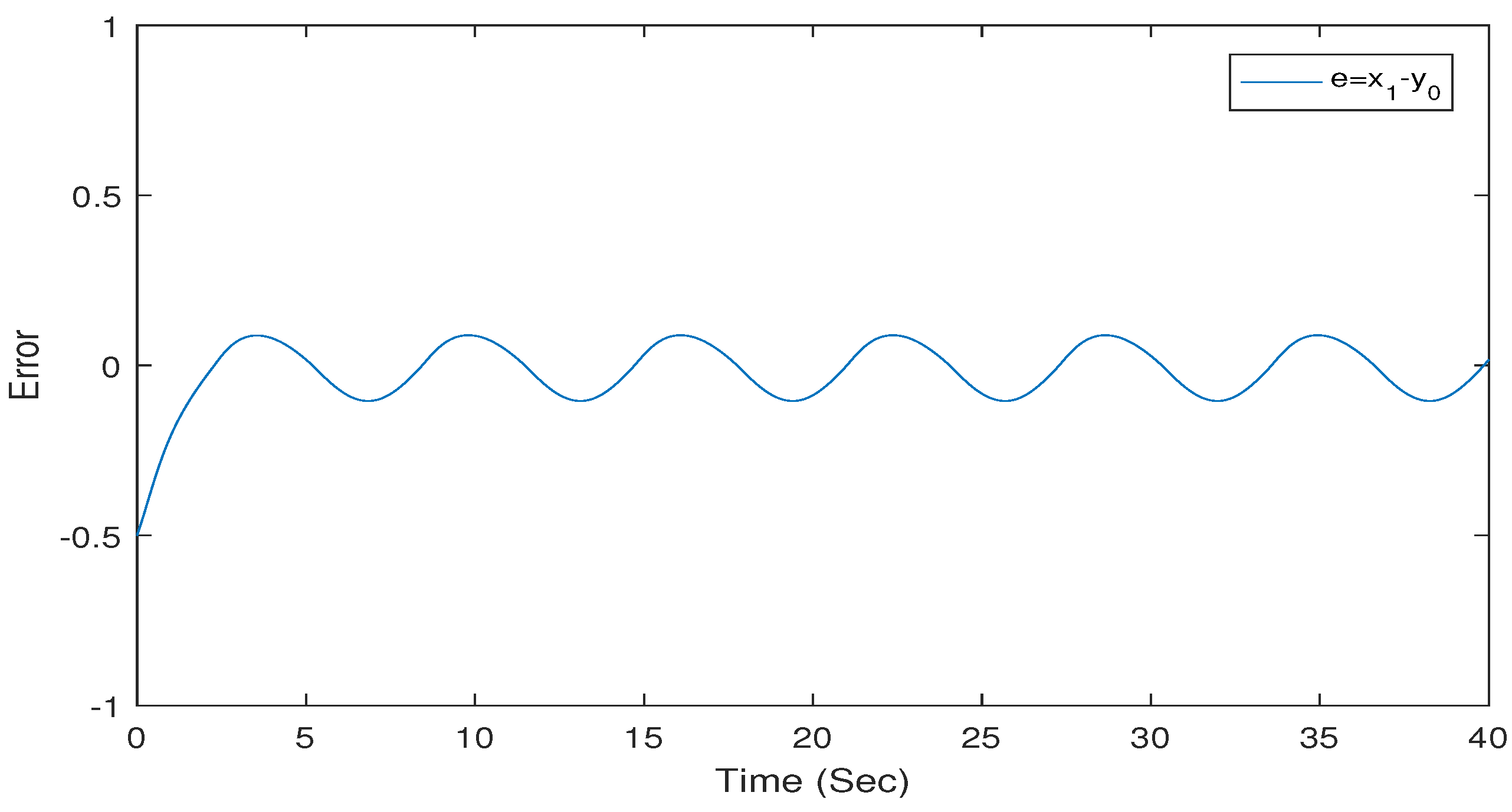
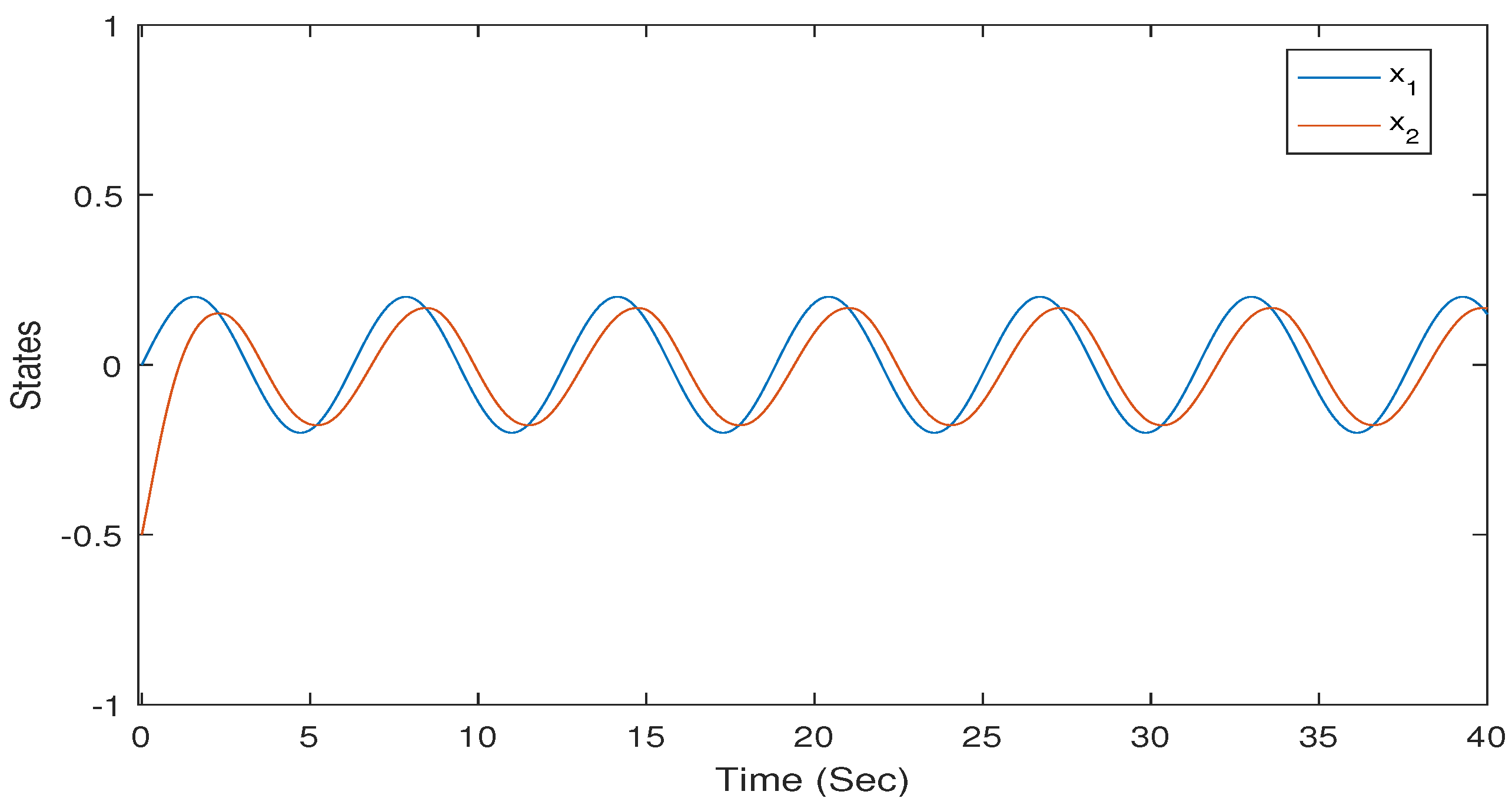
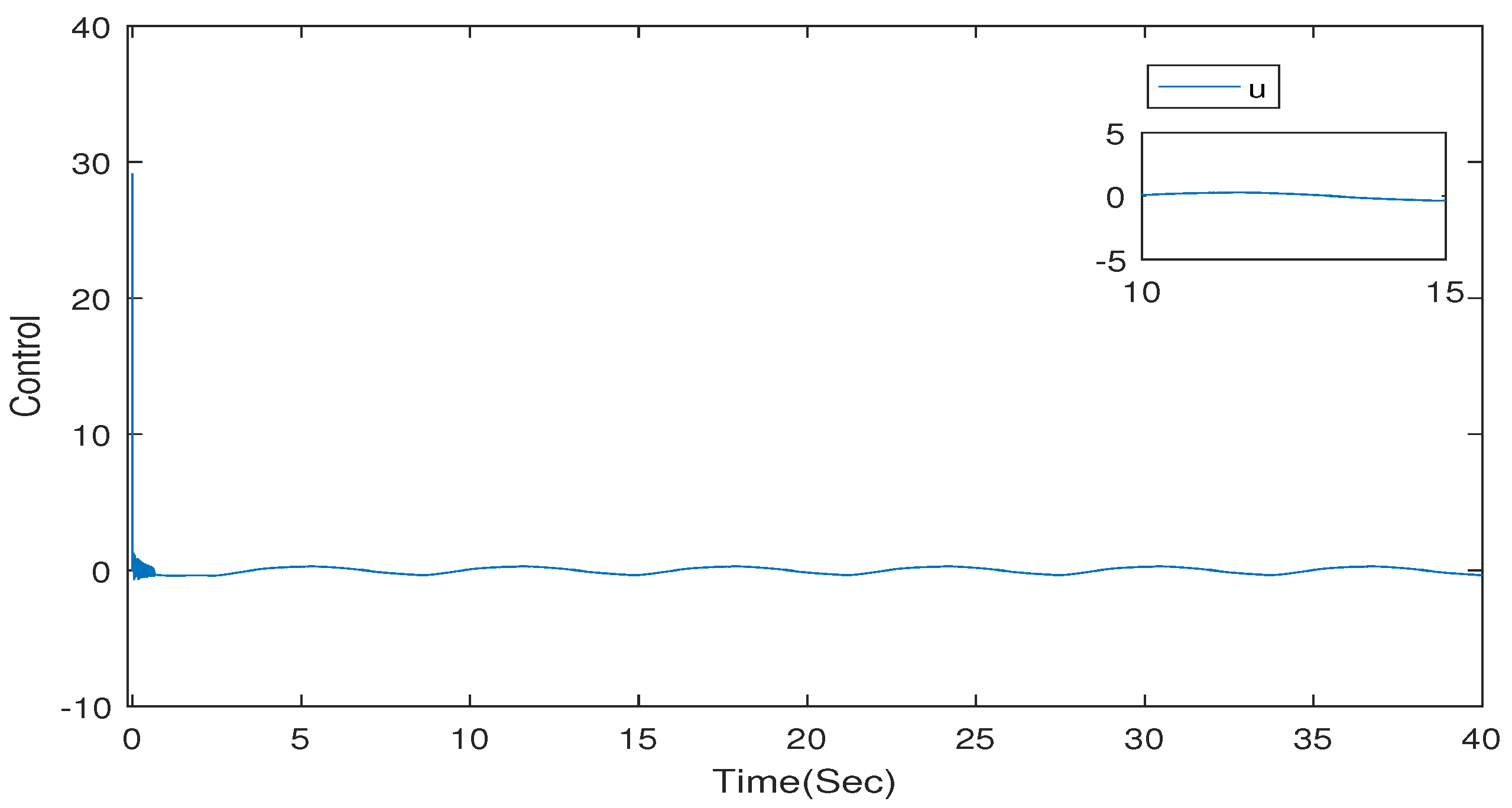
By randomly choosing parameters $c_1=1.3$, $c_2=1$, and a set of initial values ${(x_1(0),x_2(0))}^T={(-0.5,0.6)}^T$. Through the actual simulation, the system responses of the tracking error, states, and controller are shown in Figure 1, Figure 2 and Figure 3. It can be seen from Figure 1 that when $\forall t>T=2s$, the error $|e|=|x_1-y_0|<0.1$. At the same time, the effectiveness of the design idea can be directly illustrated with Figure 2 and Figure 3.

4. Conclusions

We studied the output tracking problem of RNSs with time-varying powers. The advantage of our control is that both time-varying power and SOMP are considered, which is more practical than the existing results, which only consider one factor. First, different from the deterministic systems considered in [15], the disturbance of the system studied in this paper is characterized by SOMP. The difference between the SOMP and Gaussian white noise is that white noise is an independent random process, while the SOMP is an interrelated random process. Secondly, the power of the system studied in this paper is a function of the time-varying order, which must be taken into account in the construction of the controller. The time-invariant controller was designed. It is concluded that the expectation of the fourth moment of the tracking deviation can be trimmed to be arbitrarily small, and all states are bounded in probability.

There are some future research topics, e.g., when there is uncertainty in the system, how to design the controller to ensure the tracking performance, or to generalize the results in this paper to more general systems in [28,29,30,31] or a more practical system [32].

References

- Zhang, T.P.; Xiao, X.N. Adaptive output feedback tracking control of stochastic nonlinear systems with dynamic uncertainties. Int. J. Robust Nonlin. 2015, 25, 1282–1300. [Google Scholar] [CrossRef]
- Li, W.Q.; Krstic, M. Stochastic adaptive nonlinear control with filterless least-squares. IEEE Trans. Autom. Control 2021, 66, 3893–3905. [Google Scholar] [CrossRef]
- Niu, B.; Wang, D.; Alotaibi, N.D.; Alsaadi, F.E. Adaptive neural state-feedback tracking control of stochastic nonlinear switched systems: An average dwell-time method. IEEE Trans. Neur. Net. Learn. 2019, 30, 1076–1087. [Google Scholar] [CrossRef] [PubMed]
- Jin, S.L.; Liu, Y.G.; Man, Y.C. Global output-feedback stabilization for stochastic nonlinear systems with function control coefficients. Asian J. Control 2016, 18, 1189–1199. [Google Scholar] [CrossRef]
- Li, W.Q.; Krstic, M. Mean-nonovershooting control of stochastic nonlinear systems. IEEE Trans. Autom. Control 2021, 66, 5756–5771. [Google Scholar] [CrossRef]
- Li, W.Q.; Krstic, M. Stochastic nonlinear prescribed-time stabilization and inverse optimality. IEEE Trans. Autom. Control 2022, 67, 1179–1193. [Google Scholar] [CrossRef]
- Cui, R.H.; Xie, X.J. Finite-time stabilization of stochastic low-order nonlinear systems with time-varying orders and FT-SISS inverse dynamics. Automatica 2021, 125, 109418. [Google Scholar] [CrossRef]
- Naifar, O.; Ben, M.A.; Hammami, M.A.; Ouali, A. On Observer Design for a Class of Nonlinear Systems Including Unknown Time-Delay. Mediterr. J. Math. 2016, 13, 2841–2851. [Google Scholar] [CrossRef]
- Jmal, A.; Ben Makhlouf, A.; Nagy, A.M.; Naifar, O. Finite-time stability for Caputo–Katugampola fractional-order time-delayed neural networks. Neural Process. Lett. 2019, 50, 607–621. [Google Scholar] [CrossRef]
- Cui, R.H.; Xie, X.J. Finite-time stabilization of output-constrained stochastic high-order nonlinear systems with high-order and low-order nonlinearities. Automatica 2022, 136, 110085. [Google Scholar] [CrossRef]
- Cui, R.H.; Xie, X.J. Adaptive state-feedback stabilization of state-constrained stochastic high-order nonlinear systems. Sci. China Inf. Sci. 2021, 64, 200203. [Google Scholar] [CrossRef]
- Peng, J.M.; Wang, J.N.; Shan, J.Y. Robust cooperative output tracking of networked high-order power integrators systems. Int. J. Control 2016, 89, 270–280. [Google Scholar] [CrossRef]
- Liu, J.Z.; Yan, S.; Zeng, D.L.; Lv, Y. A dynamic model used for controller design of a coal fired once-through boiler-turbine unit. IEEE Trans. Auto. Control 2015, 93, 2069–2078. [Google Scholar] [CrossRef]
- Rui, C.; Reyhangolu, M.; Kolmanovsky, I.; McClamroch, N.H. Nonsmooth stabilization of an underactuated unstable two degrees of freedom mechanical system. In Proceedings of the 36th IEEE Conference on Decision and Control, San Diego, CA, USA, 10–12 December 1997; Volume 4, pp. 3998–4003. [Google Scholar] [CrossRef]
- Li, W.Q.; Liu, Y.; Yao, X.X. State-feedback stabilization and inverse optimal control for stochastic high-order nonlinear systems with time varying powers. Asian J. Control 2021, 23, 739–750. [Google Scholar] [CrossRef]
- Man, Y.C.; Liu, Y.G. Global adaptive stabilization and practical tracking for nonlinear systems with unknown powers. Automatica 2019, 100, 171–181. [Google Scholar] [CrossRef]
- Bertram, J.; Sarachik, P. Stability of circuits with randomly timevarying parameters. IRE Trans. Circuit Theory 1959, 6, 260–270. [Google Scholar] [CrossRef]
- Soong, T.T. Random Differential Equations in Science and Engineering. Math. Sci. Eng. 1973, 103. [Google Scholar] [CrossRef] [Green Version]
- Wu, Z.J. Stability criteria of random nonlinear systems and their applications. IEEE Trans. Autom. Control. 2015, 60, 1038–1049. [Google Scholar] [CrossRef]
- Wu, Z.J.; Karimi, H.R.; Shi, P. Practical trajectory tracking of random Lagrange systems. Automatica 2019, 105, 314–322. [Google Scholar] [CrossRef]
- Yao, L.Q.; Zhang, W.H. Adaptive tracking of random nonlinear system. Int. J. Robust Nonlin. 2017, 27, 3833–3840. [Google Scholar] [CrossRef]
- Wu, Z.J.; Wang, S.T.; Cui, M.Y. Tracking controller design for random nonlinear benchmark system. J. Frank. Inst. 2017, 354, 360–371. [Google Scholar] [CrossRef]
- Li, W.Q.; Liu, L.; Feng, G. Cooperative control of multiple nonlinear benchmark systems perturbed by second-order moment processes. IEEE Trans. Cybern. 2020, 50, 902–910. [Google Scholar] [CrossRef] [PubMed]
- Yao, L.Q.; Zhang, W.H.; Xie, X.J. Stability analysis of random nonlinear systems with time-varying delay and its application. Automatica 2021, 117, 108994. [Google Scholar] [CrossRef] [Green Version]
- Jiao, T.C.; Zheng, H.C.; Xu, S.Y. Unified stability criteria of random nonlinear time-varying impulsive switched systems. IEEE Trans. Circuits Syst. I 2020, 67, 3099–3112. [Google Scholar] [CrossRef]
- Shan, Q.H.; Zhang, H.G.; Wang, Z.S.; Zhang, Z. Global asymptotic stability and stabilization of neural networks with general noise. IEEE Trans. Neur. Net. Lear. 2018, 29, 597–607. [Google Scholar] [CrossRef]
- Chen, C.C.; Qian, C.J.; Lin, X.Z.; Sun, Z.Y.; Liang, Y.W. Smooth output feedback stabilization for a class of nonlinear systems with time-varying powers. Int. J. Robust Nonlinear Control. 2017, 27, 5113–5128. [Google Scholar] [CrossRef]
- Huang, H.; Shirkhani, M.; Tavoosi, J.; Mahmoud, O. A New Intelligent Dynamic Control Method for a Class of Stochastic Nonlinear Systems. Mathematics 2022, 10, 1406. [Google Scholar] [CrossRef]
- Zhu, C.; He, L.; Zhang, K.; Sun, W.; He, Z. Optimal Timing Fault Tolerant Control for Switched Stochastic Systems with Switched Drift Fault. Mathematics 2022, 10, 1880. [Google Scholar] [CrossRef]
- Li, W.Q.; Yao, X.X.; Krstic, M. Adaptive-gain observer-based stabilization of stochastic strict-feedback systems with sensor uncertainty. Automatica 2020, 120, 109112. [Google Scholar] [CrossRef]
- Li, W.Q.; Krstic, M. Prescribed-time output-feedback control of stochastic nonlinear systems. IEEE Trans. Autom. Control. 2022, 68. [Google Scholar] [CrossRef]
- Ayadi, M.; Naifar, O.; Derbel, N. High-order sliding mode control for variable speed PMSG-wind turbine-based disturbance observer. Int. J. Model. Identif. Control. 2019, 32, 85–92. [Google Scholar] [CrossRef]
Figure 1.
Response to the tracking error.
Figure 2.
Response of the states.
Figure 3.
Response of the controller.
Publisher’s Note: MDPI stays neutral with regard to jurisdictional claims in published maps and institutional affiliations. |
© 2022 by the authors. Licensee MDPI, Basel, Switzerland. This article is an open access article distributed under the terms and conditions of the Creative Commons Attribution (CC BY) license (https://creativecommons.org/licenses/by/4.0/).
Share and Cite
MDPI and ACS Style
Wang, R.; Wang, H.; Li, W.; Niu, B. Output Tracking Control of Random Nonlinear Time-Varying Systems. Mathematics 2022, 10, 2524. https://0-doi-org.brum.beds.ac.uk/10.3390/math10142524
AMA Style
Wang R, Wang H, Li W, Niu B. Output Tracking Control of Random Nonlinear Time-Varying Systems. Mathematics. 2022; 10(14):2524. https://0-doi-org.brum.beds.ac.uk/10.3390/math10142524
Chicago/Turabian StyleWang, Ruitao, Hui Wang, Wuquan Li, and Ben Niu. 2022. "Output Tracking Control of Random Nonlinear Time-Varying Systems" Mathematics 10, no. 14: 2524. https://0-doi-org.brum.beds.ac.uk/10.3390/math10142524
Note that from the first issue of 2016, this journal uses article numbers instead of page numbers. See further details here.