Reconstructing the Local Volatility Surface from Market Option Prices

Abstract

We present an efficient and accurate computational algorithm for reconstructing a local volatility surface from given market option prices. The local volatility surface is dependent on the values of both the time and underlying asset. We use the generalized Black–Scholes (BS) equation and finite difference method (FDM) to numerically solve the generalized BS equation. We reconstruct the local volatility function, which provides the best fit between the theoretical and market option prices by minimizing a cost function that is a quadratic representation of the difference between the two option prices. This is an inverse problem in which we want to calculate a local volatility function consistent with the observed market prices. To achieve robust computation, we place the sample points of the unknown volatility function in the middle of the expiration dates. We perform various numerical experiments to confirm the simplicity, robustness, and accuracy of the proposed method in reconstructing the local volatility function.

1. Introduction

In 1973, Fischer Black and Myron Scholes first introduced the Black–Scholes (BS) equation for option pricing [1]:

$$\begin{array}{c}\hfill \frac{\partial u(S,t)}{\partial t}+\frac{1}{2}{\left(\sigma S\right)}^2\frac{{\partial }^{2}u(S,t)}{\partial S^2}+rS\frac{\partial u(S,t)}{\partial S}-ru(S,t)=0,\end{array}$$

(1)

where $u(S,t)$ is the option value, S is the underlying price, t is the time variable, $\sigma$ is the volatility of S, and r is the short interest rate. Equation (1) is solved using boundary conditions and a payoff condition at time $t=T$. The BS equation was derived under the assumption of constant volatility. However, it is widely known that the BS equation with constant volatility cannot accurately produce market option prices. In general, as volatility increases, the prices of options also tend to rise because of the increasing chances of options ending in the money. The volatility and option prices are positively correlated with each other. A generalized BS model was proposed to overcome the limitations of the BS equation with a constant volatility term:

$$\begin{array}{c}\hfill \frac{\partial u(S,t)}{\partial t}+\frac{1}{2}{\left[\sigma (S,t)S\right]}^2\frac{{\partial }^{2}u(S,t)}{\partial S^2}+rS\frac{\partial u(S,t)}{\partial S}-ru(S,t)=0,\end{array}$$

(2)

where $\sigma (S,t)$ is the space- and time-dependent volatility function [2]. Here, we call $\sigma (S,t)$ by the local volatility function because it is a function of both the asset price S and time t, which is a generalization of the constant volatility. Implied volatility is the volatility calculated by inputting the market option price, strike, current underlying asset price, maturity time, and interest rate into the BS equation with a constant volatility, which makes both the theoretical and market option prices the same. Therefore, the implied volatility is the function of the market option price, strike, current underlying asset price, maturity time, and interest rate. We can construct an implied volatility surface by changing strike prices and maturity times while fixing the other parameter values. Note that we are interested in constructing a local volatility function, which is a function of the asset price S and time t not strike price and time.

Various studies have been conducted on reconstructing volatility surfaces using market option prices. Jin et al. [3] proposed a reconstruction method for a non-constant volatility model using the BS equation. Georgiev and Vulkov [4] developed a fast and efficient computational method for reconstructing the time-dependent local volatility surface and used a predictor-corrector scheme because of the non-uniqueness of the local volatility surface. Hofmann et al. [5] developed a simultaneous reconstruction of volatility and interest rate functions from call-and put-price functions and overcame the ill-posedness using a two-parameter Tikhonov regularization. Georgiev and Vulkov [6] also considered the simultaneous recovery of the temporally changing volatility and interest rate functions. Using the BS model, Park et al. [7] proposed a calibration technique of the time-dependent volatility and interest rate functions. Zhang et al. [8] reconstructed the local volatility function using Dupire’s equation with total variation regularization. In quantitative finance, the reconstruction of local volatility is an important inverse problem [9]. In [2], the authors studied the inverse problem of solving a time-dependent local volatility function using option prices. In [10,11], the authors proposed local volatility function reconstruction algorithms that use an effective region of volatility. In [12], the authors presented a simple and efficient algorithm using a jump-diffusion model to calculate time-dependent volatility. Recently, deep learning has been attracting attention from the financial field, and a large part of it has been used for financial time series prediction [13]. Pradeepkumar and Ravi [14] proposed a neural network method for predicting the volatility of financial time series and verified its superior performance compared to several other machine learning methods. Hellmuth and Klingenberg [15] presented a numerical variation based on Bi-Fidelity on a machine learning method. Option pricing studies [16,17,18] on various financial products have been conducted, as well as option pricing studies [19,20,21] on the BS equation.

The primary contribution of this paper is to propose a simple, efficient, and accurate computational method for reconstructing the local volatility function using only given market option prices, expiration times, strike prices, and the generalized BS equation. Some assumptions and additional requirements in the existing literature are Tikhonov regularization, Dupire’s equation, and effective region of volatility. Compared to the previous methods, which involve several assumptions and additional requirements for reconstructing the local volatility function, the proposed algorithm only uses the minimum requirements. Therefore, it is one of the simplest reconstruction methods for the local volatility function.

The layout of this paper is as follows. In Section 2, we present the proposed algorithm for optimizing the local volatility function. In Section 3, computational experiments are performed to demonstrate the efficiency and accuracy of the proposed algorithm. Finally, in Section 4, conclusions are presented.

2. Methodology

We now briefly describe the proposed algorithm of optimizing the local volatility function. We use the generalized BS Equation (2) to reconstruct the local volatility function $\sigma (S,t)$ from market option prices. Equation (2) can be rewritten as

$$\frac{\partial u(S,\tau )}{\partial \tau }=\frac{1}{2}{\left[\sigma (S,\tau )S\right]}^2\frac{{\partial }^{2}u(S,\tau )}{\partial S^2}+rS\frac{\partial u(S,\tau )}{\partial S}-ru(S,\tau ),$$

(3)

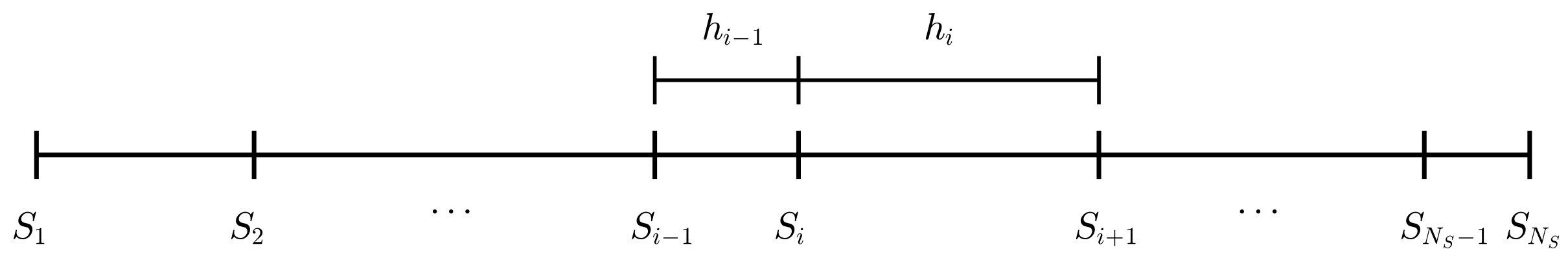
for $(S,\tau )\in \Omega \times (0,T]$ with initial condition $u(S,0)$, where $\tau =T-t$. We numerically solve Equation (3) using the finite difference scheme. Let $u_i^n\equiv u(S_i,n\Delta \tau )$ be the numerical solution of Equation (3) for $i=1,2,\dots ,N_S$ and $n=0,1,\dots ,N_{\tau }$. In this study, unless otherwise specified, we use a uniform temporal size $\Delta \tau =1/360$. We use the non-uniform asset price discrete domain as shown in Figure 1. Here, $h_i=S_{i+1}-S_i$ and $S_1=0$.

Let ${\sigma }_i^n\equiv \sigma (S_i,n\Delta \tau )$ be discrete variable volatility. Using the implicit Euler method, we discretize Equation (3) as follows:

$$\begin{array}{ccc}& & \frac{u_i^{n+1}-u_i^n}{\Delta \tau }=\frac{{\left({\sigma }_i^{n+1}{S}_i\right)}^2}{2}\left(\frac{2u_{i-1}^{n+1}}{h_{i-1}(h_i+h_{i-1})}-\frac{2u_i^{n+1}}{h_i{h}_{i-1}}+\frac{2u_{i+1}^{n+1}}{h_i(h_i+h_{i-1})}\right)\hfill \\ & & +r{S}_i\left(\frac{-h_i{u}_{i-1}^{n+1}}{h_{i-1}(h_i+h_{i-1})}+\frac{(h_i-h_{i-1})u_i^{n+1}}{h_{i-1}{h}_i}+\frac{h_{i-1}{u}_{i+1}^{n+1}}{h_i(h_{i-1}+h_i)}\right)-r{u}_i^{n+1}.\hfill \end{array}$$

(4)

We can then rewrite Equation (4) as

$${\alpha }_i{u}_{i-1}^{n+1}+{\beta }_i{u}_i^{n+1}+{\gamma }_i{u}_{i+1}^{n+1}=b_i,fori=2,\cdots ,N_S,$$

(5)

where

$$\begin{array}{ccc}\hfill {\alpha }_i& =& \frac{r{S}_i{h}_i-{\left({\sigma }_i^{n+1}{S}_i\right)}^2}{h_{i-1}(h_i+h_{i-1})},{\beta }_i=\frac{1}{\Delta \tau }-\frac{r{S}_i(h_i-h_{i-1})-{\left({\sigma }_i^{n+1}{S}_i\right)}^2}{h_{i-1}{h}_i}+r,\hfill \\ \hfill {\gamma }_i& =& -\frac{S_i{h}_{i-1}}{h_i(h_{i-1}+h_i)}-\frac{{\left({\sigma }_i^{n+1}{S}_i\right)}^2}{h_i(h_{i-1}+h_i)},b_i=\frac{u_i^n}{\Delta \tau }.\hfill \end{array}$$

We use the zero Dirichlet boundary condition at $S_1$, that is, $u_1^{n+1}=0$, and linearity condition at $S_{N_S}$, that is, $u_{N_S+1}^{n+1}=2u_{N_S}^{n+1}-u_{N_S-1}^{n+1}$, for all n [22]. To numerically solve the discrete system (5), we use the Thomas algorithm [23]. Note that the generalized BS equation is a degenerate parabolic partial differential equation and has a zero coefficient in front of the partial derivatives at $S_1=0$. However, we use the homogeneous Dirichlet boundary condition at $S_1$; therefore, we do not encounter a degenerate problem. In addition, we assume a positive local volatility function. Let us assume that we have market option prices $\left\{U_{\beta }^{\alpha }\right\}$ at $T_{\alpha }$ for $\alpha =1,\dots ,M_{\alpha }$ and exercise prices $K_{\beta }$ for $\beta =1,\dots ,M_{\beta }$. Here, $T_1<\dots <T_{M_{\alpha }}$ and $K_1<\cdots <K_{M_{\beta }}$. Using the given option prices $\left\{U_{\beta }^{\alpha }\right\}$, we compute the local volatility function $\sigma (S,t)$ by minimizing the following mean-square error (MSE) [10]:

$$\mathcal{E}\left(\sigma \right)=\frac{1}{M_{\alpha }{M}_{\beta }}\sum _{\alpha =1}^{M_{\alpha }}\sum _{\beta =1}^{M_{\beta }}{\omega }_{\beta }^{\alpha }{[u_{K_{\beta }}(\sigma ;S_0,T_{\alpha })-U_{\beta }^{\alpha }]}^2,$$

(6)

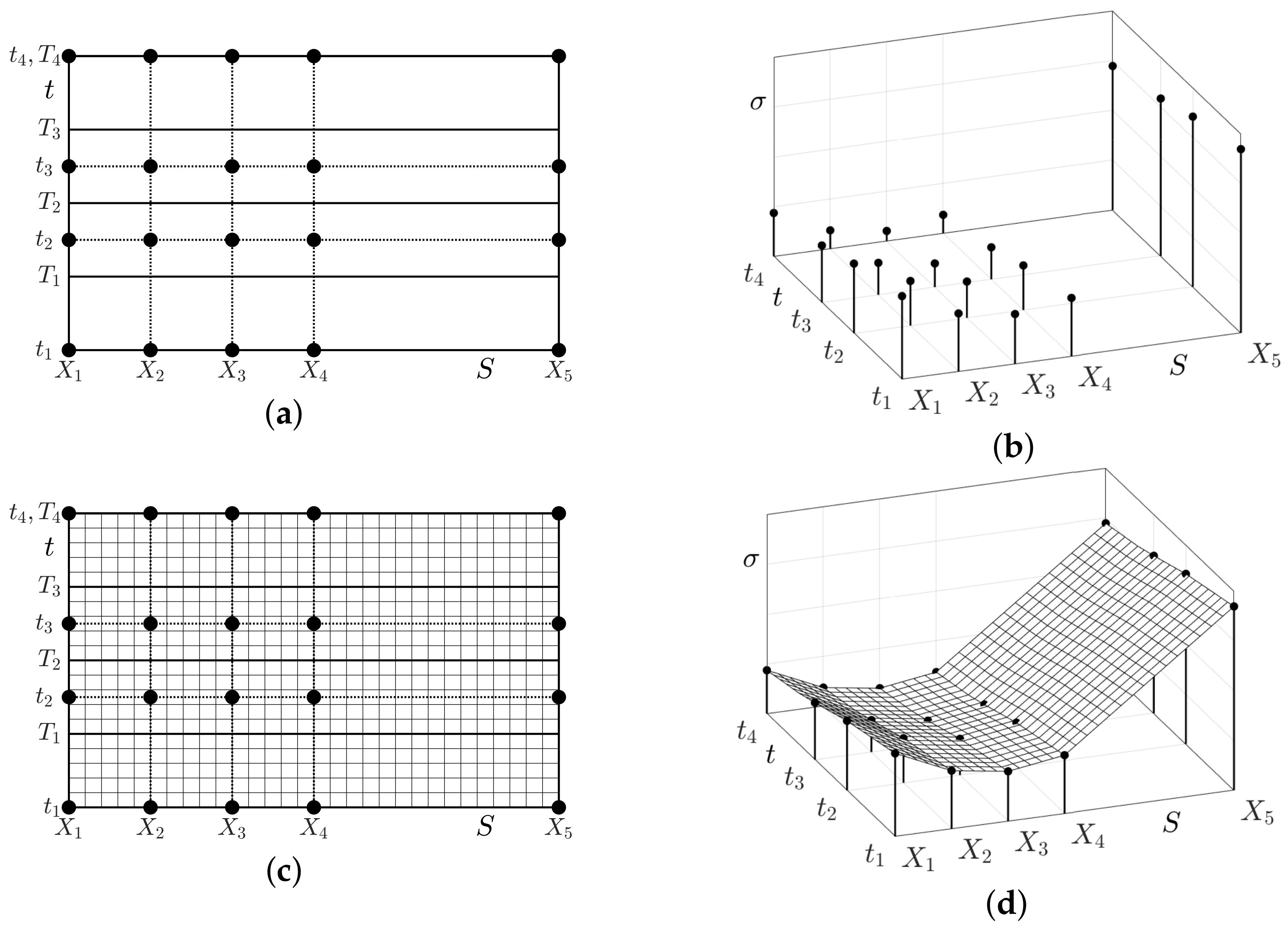
where $u_{K_{\beta }}(\sigma ;S_0,T_{\alpha })$ is the computational solution at $S=S_0$ of Equation (3) with strike price $K_{\beta }$ at time $T_{\alpha }$ and initial condition $u_i^0=max(S_i-K_{\beta },0)$ for $i=1,2,\dots ,N_S$. Here, ${\omega }_{\beta }^{\alpha }$ is one if market data are used; zero otherwise. We apply the lsqcurvefit function in MATLAB R2021a [24] to compute the optimal volatility function $\sigma$ that minimizes cost function $\mathcal{E}\left(\sigma \right)$. To achieve robust computation, we place points of the unknown volatility function at the middle times of the expiration dates [3]. We use the following notation $t_1=0$; $t_q=(T_{q-1}+T_q)/2$ for $q=2,\dots ,M_{\alpha }-1$ and $t_{M_{\alpha }}=T_{M_{\alpha }}$, as shown in Figure 2a.

Let us define the piecewise linearly interpolated volatility function $\sigma (S,t)$ that satisfies

$$\begin{array}{c}\hfill \sigma (S,t)={\sigma }_{pq} \mathrm{if} S=X_p \mathrm{and} t=t_q,\end{array}$$

where $(X_p,t_q)$ are the sample points and ${\sigma }_{pq}$ are the sample volatility values at the sample points, as shown in Figure 2b. Figure 2c,d show the grid used in the finite difference method and the interpolated volatility values at the grid of query points, respectively.

The superior properties of the proposed method are its simplicity, efficiency, and accuracy in reconstructing the local volatility function using only the given market option prices, strike prices, expiration times, and generalized BS equation. For interested readers, MATLAB code with a uniform grid size is provided in the Appendix A.

3. Computational Experiments

We present several numerical experiments to demonstrate the effectiveness of the proposed algorithm. We also provide the CPU times using an Intel(R) Core(TM) i9-12900K CPU 3.19 GHz processor for each experiment.

3.1. Effect of Initial Guess of $\sigma (S,t)$

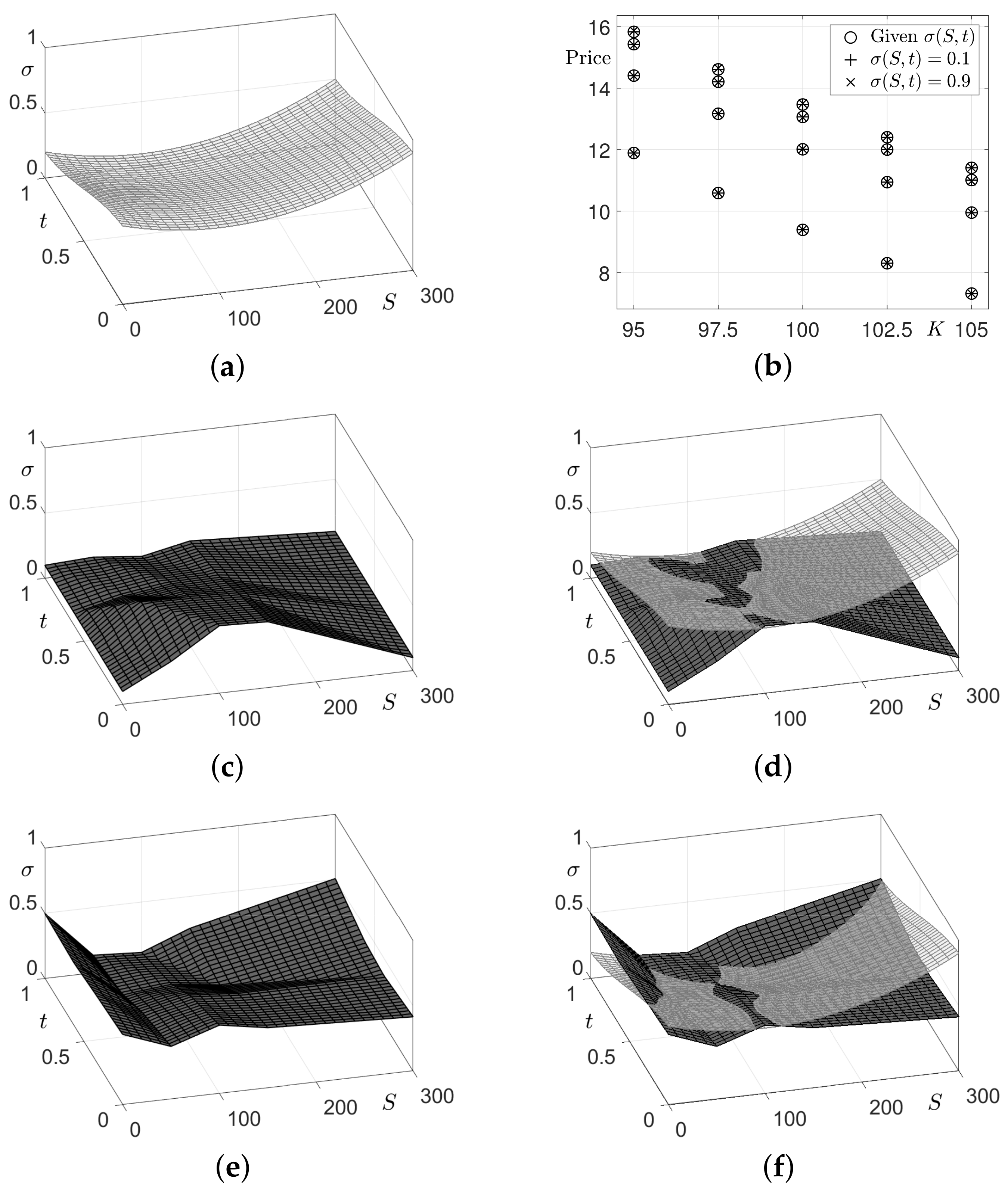
First, we examine the effect of the initial guess of $\sigma (S,t)$ on reconstructing the local volatility function. As a test problem, we consider the following local volatility function on $\Omega =(0,3S_0)\times (0,1)$; see Figure 3a:

$$\begin{array}{c}\hfill \sigma (S,t)=0.00001{(S-S_0)}^2+0.1cos\left(\pi t\right)-0.2t+0.4,\end{array}$$

(7)

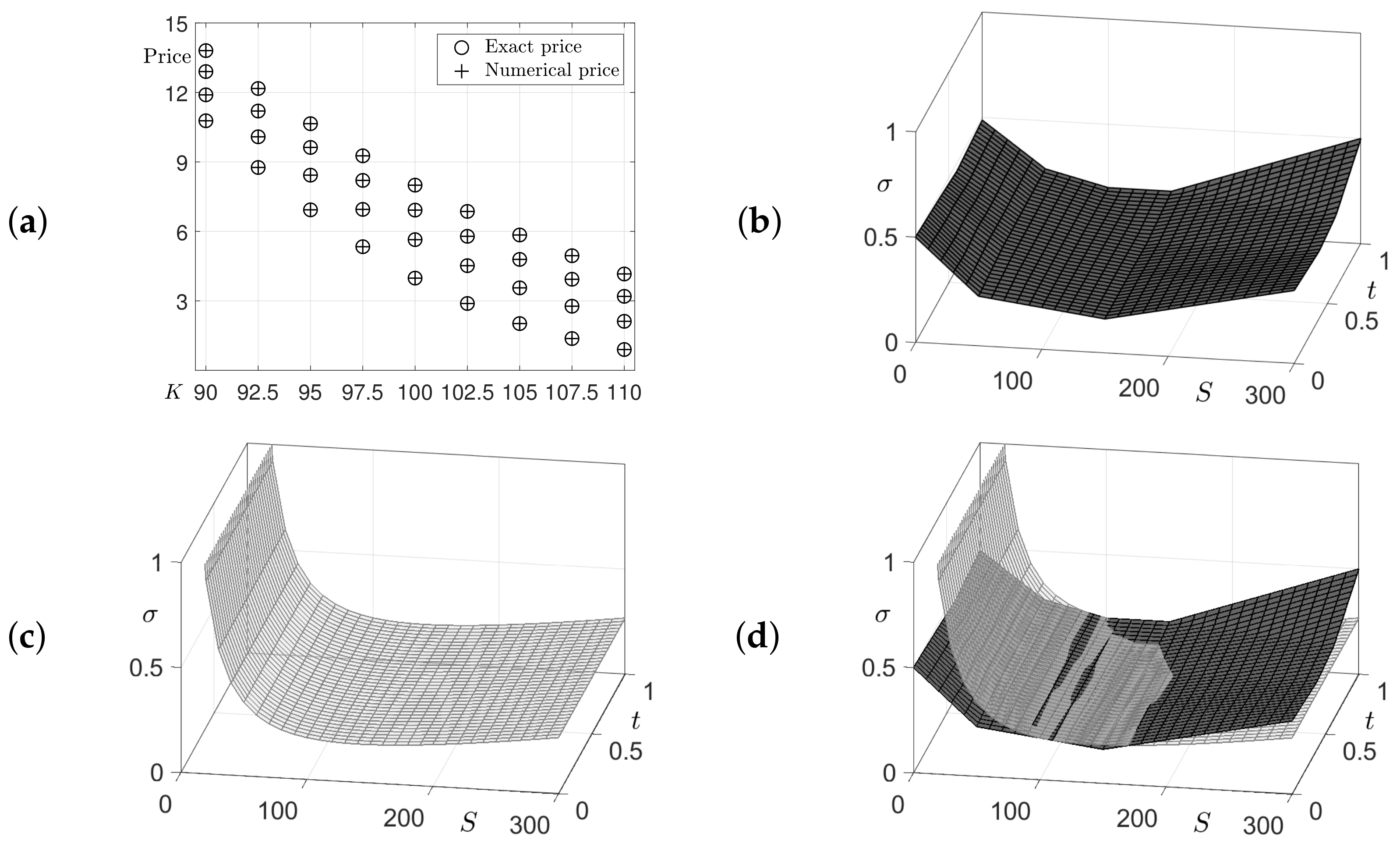
where $S_0=100$. The parameters used are $\Delta \tau =1/360$, $N_S=301$, $r=0.01$, $T_{\alpha }=0.25\alpha$ for $\alpha =1,2,3,4$, and strike prices $K_{\beta }=92.5+2.5\beta$ for $\beta =1,2,\cdots ,5$. Using these parameter values, we generate market call option prices $\left\{U_{\beta }^{\alpha }\right\}$ for $\alpha =1,2,3,4$ and $\beta =1,2,3,4,5$. Figure 3b shows the option prices computed using the given volatility function (7) and two reconstructed local volatility functions with different initial guesses. Figure 3c,e are the reconstructed volatility surfaces using initial guesses $\sigma (S,t)=0.1$ and $\sigma (S,t)=0.9$, respectively. Figure 3d,f are the overlapped surfaces of (c) and (e) with the given reference volatility function, respectively.

These results are in good agreement with each other in the effective volatility region, which is computed using the probability density function of a log-normal distribution to define the effective area. The existence of the effective domain is mainly due to the fact that the volatility term in the BS equation (2) is close to zero where the second derivatives of the option prices are small. In the case of call options, the option prices are close to linearly far away from the strike prices. As schematically shown in Figure 4, the boundary of the effective volatility region is a parabola-type shape; see [10] for more details.

Because the results are virtually independent of the initial guess, we will use $\sigma (S,t)=0.5$ as an initial guess for reconstructing the local volatility function from now on. When $\sigma =0.1$ and $\sigma =0.9$, the CPU times for computing the local volatility functions are 36.73 and 36.04 s, respectively.

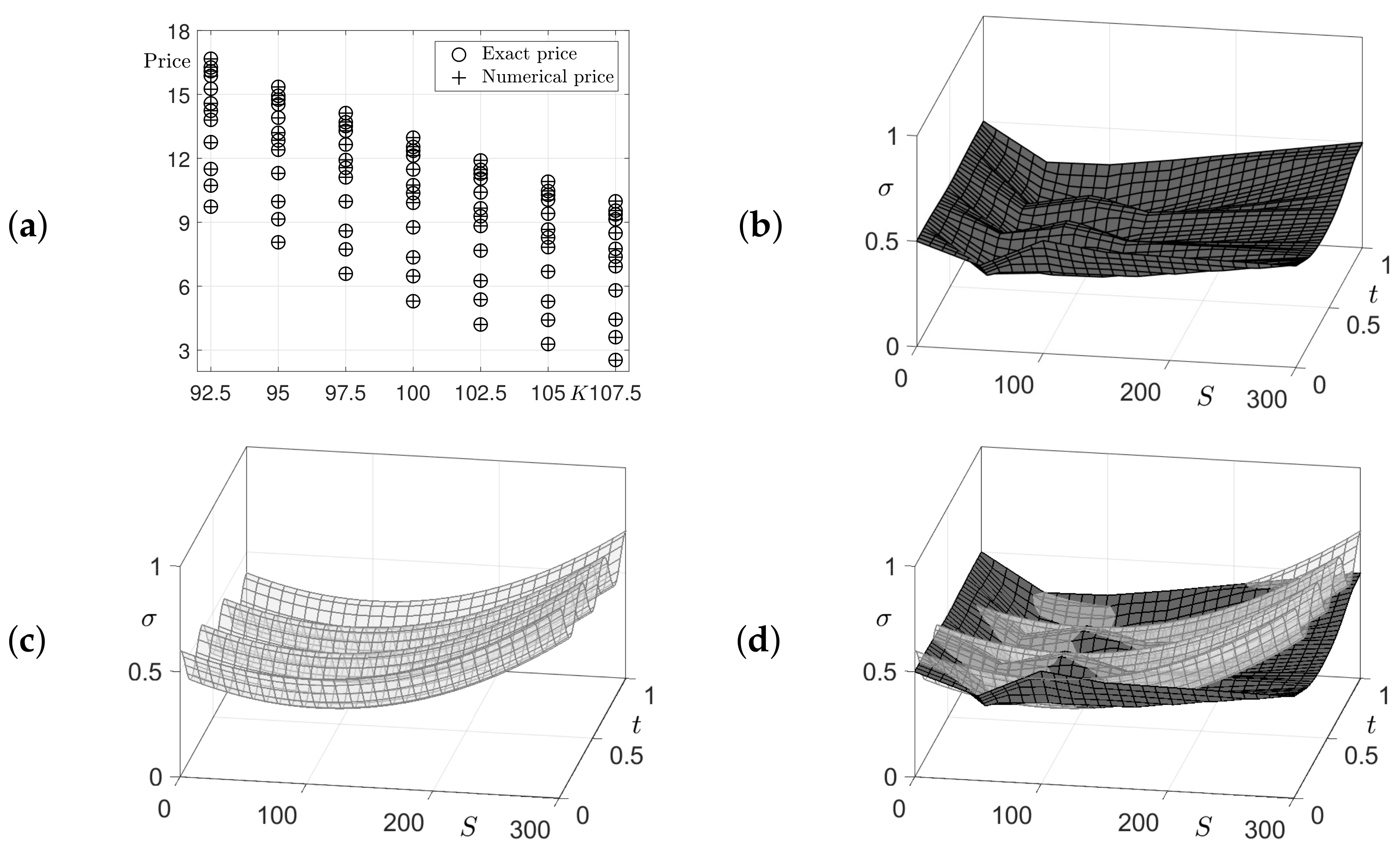
In real-world practical applications, the local volatility function from the real-world market data may have oscillations. To confirm the proposed algorithm can recover the local volatility function that can generate such function, we consider a reference local volatility function similar to that in [25] (see Figure 5c):

$$\begin{array}{c}\hfill \sigma (S,t)=\frac{2}{5}-\frac{4}{25}{e}^{\frac{t}{2}}cos\left(\frac{4\pi S}{3S_0}\right) \mathrm{on} \Omega =(0,3S_0)\times (0,1),\end{array}$$

(8)

where $S_0=100$. The parameters used are $\Delta \tau =1/360$, $N_S=301$, $r=0.01$, $T_{\alpha }=0.25\alpha$ for $\alpha =1,2,3,4$, and strike prices $K_{\beta }=75+5\beta$ for $\beta =1,2,\cdots ,9$. Figure 5a shows the option prices calculated using the given volatility function (8) and reconstructed local volatility function. Figure 5b,d are the reconstructed local volatility function and overlapped surfaces with (c), respectively. The two local volatility surfaces are in good agreement each other in the effective volatility region, which is schematically shown in Figure 4, and the computed option prices are almost identical. We can observe the proposed algorithm can recover the oscillatory local volatility function. The CPU time for computing the local volatility function is 101.27 s.

We consider another reference local volatility function, which was used in [26] (see Figure 6c):

$$\begin{array}{c}\hfill \sigma (S,t)=0.1\left(1+\frac{S_0}{S}+\frac{{(S-S_0)}^2}{100S}\right) \mathrm{on} \Omega =(0,3S_0)\times (0,1),\end{array}$$

(9)

where $S_0=100$. The parameters used are $\Delta \tau =1/360$, $N_S=301$, $r=0$, $T_{\alpha }=0.25\alpha$ for $\alpha =1,2,3,4$, and strike prices $K_{\beta }=87.5+2.5\beta$ for $\beta =1,2,\cdots ,11$. Figure 6a,b,d are the option prices computed using Equation (9) and reconstructed local volatility function, and the overlapped surfaces of the reference and reconstructed local volatility surfaces, respectively. The two local volatility surfaces are in good agreement each other in the effective volatility region, which is schematically shown in Figure 4 and the computed option prices are almost identical. The CPU time is 78.10 s.

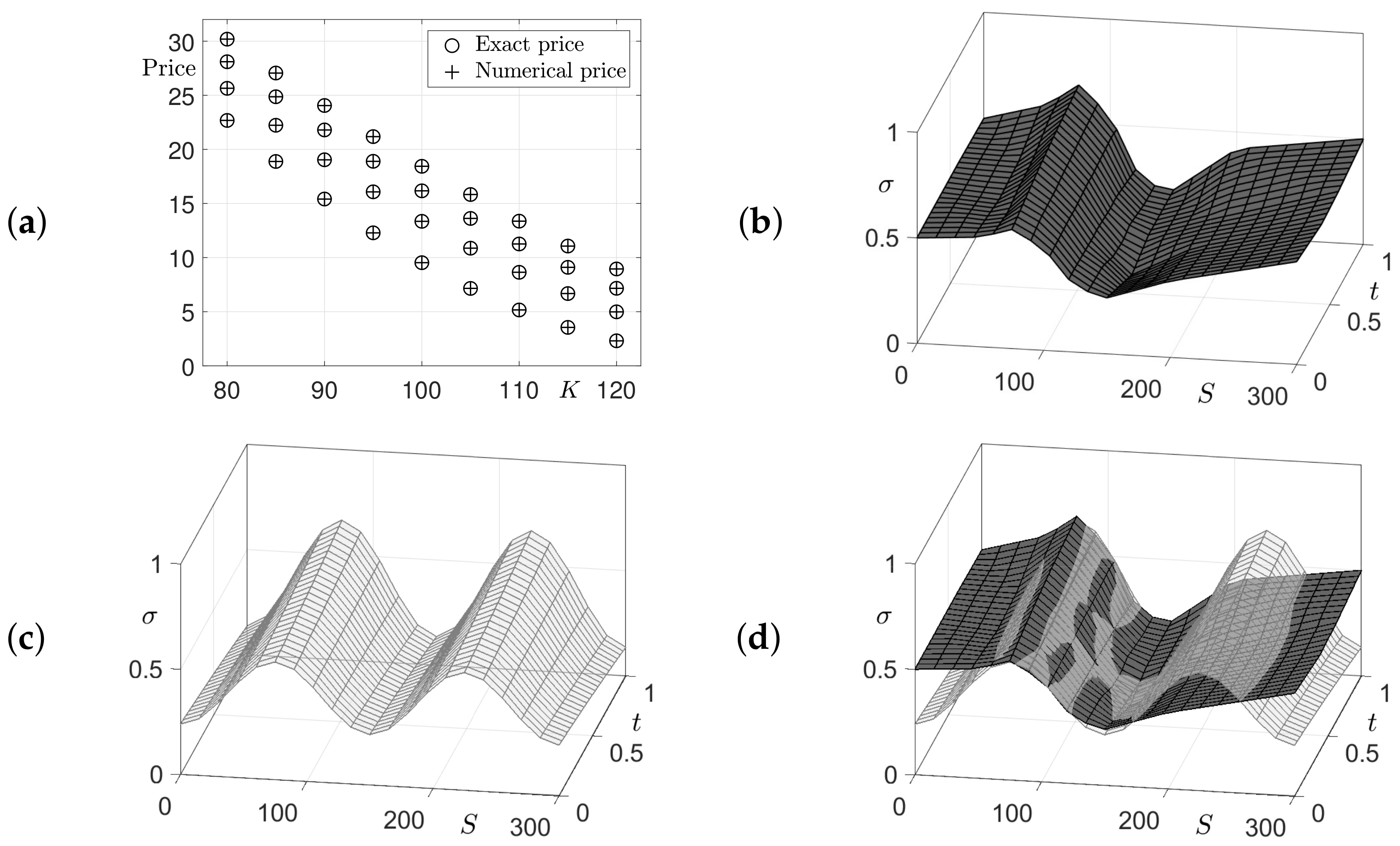
Next, we consider a more complex local volatility function on $\Omega =(0,3S_0)\times (0,1)$ with respect to the time variable (see Figure 7c):

$$\begin{array}{c}\hfill \sigma (S,t)=0.00001{(S-S_0)}^2+0.1cos\left(6\pi t\right)-0.2t+0.4,\end{array}$$

(10)

where $S_0=100$. The parameters used are $\Delta \tau =1/360$, $N_S=301$, $r=0.01$, $T_{\alpha }=\alpha /12$ for $\alpha =1,2,\cdots ,12$, and strike prices $K_{\beta }=90+2.5\beta$ for $\beta =1,2,\dots ,7$. Figure 7a,b,d are the option prices computed using Equation (10) and reconstructed local volatility function, and the overlapped surfaces of the reference and reconstructed local volatility surfaces, respectively. The two local volatility surfaces are in good agreement each other in the effective volatility region, which is schematically shown in Figure 4, and the computed option prices are almost identical. The CPU time is 369.66 s.

3.2. Local Volatility Surface from KOSPI 200 Index

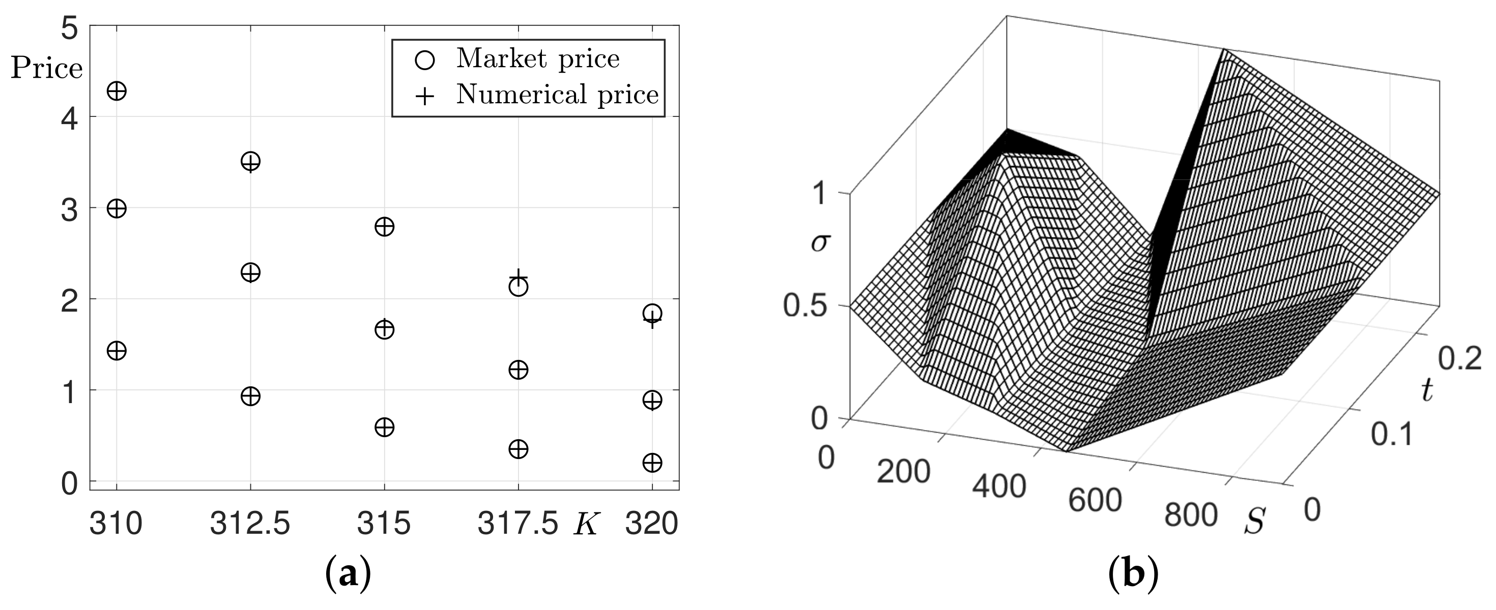
We perform a real market test using the proposed algorithm to obtain a local volatility function with KOSPI 200 index call option datasets on 14 January 2020.

Table 1. KOSPI 200 index call option prices on 14 January 2020 with respect to the strike and maturity. Our data source is the market data system of the Korea Exchange (KRX Market Data System: https://data.krx.co.kr/, accessed on 19 June 2022).

${\mathit{K}}_{\mathit{\beta }}$	310.0	312.5	315.0	317.5	320.0
$T_1=30\Delta \tau$	$1.43$	$0.93$	$0.59$	$0.35$	$0.20$
$T_2=58\Delta \tau$	$2.99$	$2.29$	$1.66$	$1.22$	$0.89$
$T_3=86\Delta \tau$	$4.28$	$3.51$	$2.79$	$2.13$	$1.84$

lists real market data with the various strikes and maturities. The strikes used in the table are $K_{\beta }=310+2.5(\beta -1)$ for $\beta =1,2,\cdots ,5$ and the maturity times are $T_1=30\Delta \tau$, $T_2=58\Delta \tau$, and $T_3=86\Delta \tau$, where $\Delta \tau =1/365$. The current value of the KOSPI 200 index is $S_0=301.53$ and the interest rate is $r=0.0149$.

Figure 8 shows the results of the proposed method by applying the real market call option prices, as listed in Table 1. We can confirm that the computational prices obtained from the proposed method are very similar to the real market values at each maturity and strike price. It can be inferred from Figure 8a,b that the proposed algorithm works well in the real market KOSPI 200 call option data. The CPU time is 9.90 s.

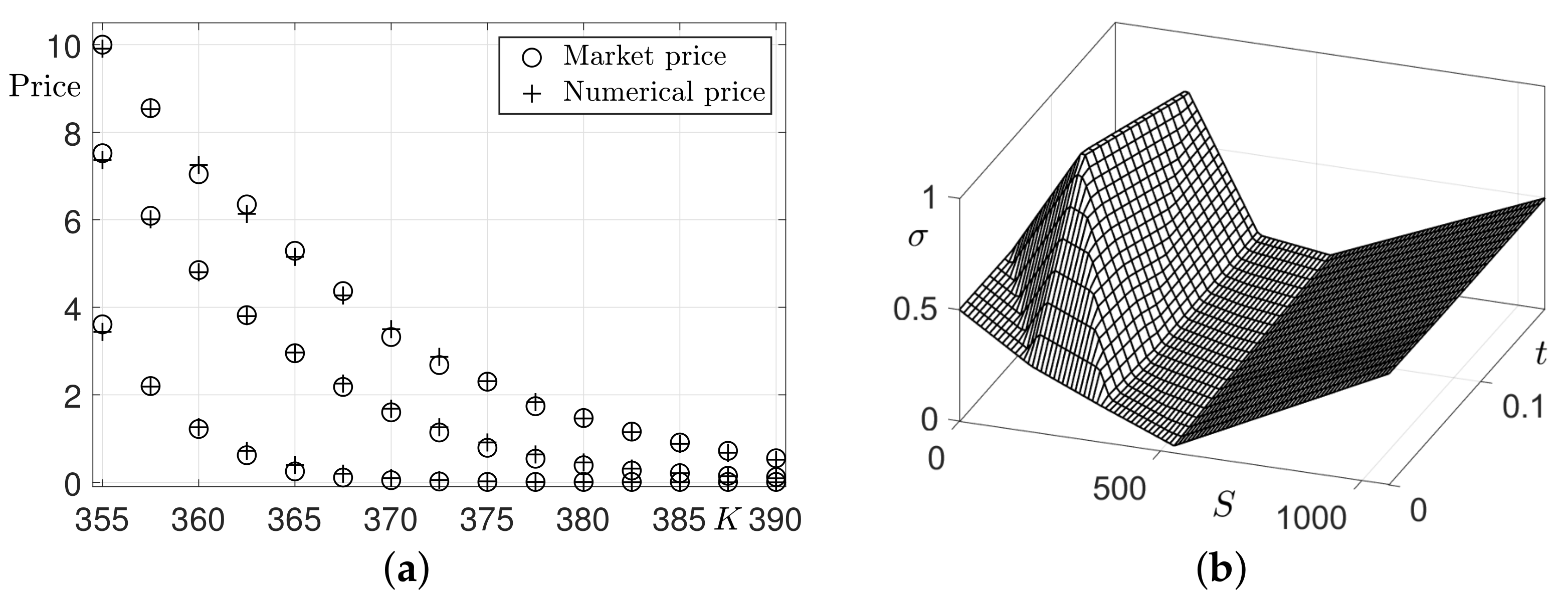
Let us consider another real-world financial test.

Table 2. KOSPI 200 index call option price on 8 April 2022 with respect to the strike and maturity. Our data source is the market data system of the Korea exchange (KRX Market Data System: https://data.krx.co.kr/, accessed on 19 June 2022).

${\mathit{K}}_{\mathit{\beta }}$	355.0	357.5	360.0	362.5	365.0	367.5	370.0	372.5	375.0	377.5	380.0	382.5	385.0	387.5	390.0
$T_1=6\Delta \tau$	$3.61$	$2.20$	$1.22$	$0.62$	$0.25$	$0.11$	$0.05$	$0.02$	$0.01$	$0.01$	$0.01$	$0.01$	$0.01$	$0.01$	$0.01$
$T_2=34\Delta \tau$	$7.52$	$6.09$	$4.85$	$3.82$	$2.95$	$2.18$	$1.60$	$1.14$	$0.79$	$0.54$	$0.39$	$0.27$	$0.21$	$0.15$	$0.12$
$T_3=62\Delta \tau$	$10.00$	$8.55$	$7.04$	$6.35$	$5.29$	$4.37$	$3.32$	$2.68$	$2.30$	$1.74$	$1.47$	$1.16$	$0.91$	$0.72$	$0.55$

lists the real market data with respect to the strikes and maturities. Strikes used in the table are $K_{\beta }=355+2.5(\beta -1)$ for $\beta =1,2,\cdots ,5$ and the maturity times are $T_1=6\Delta \tau$, $T_2=34\Delta \tau$, and $T_3=62\Delta \tau$, where $\Delta \tau =1/365$. The current value of the KOSPI 200 index is $S_0=356.01$ and interest rate is $r=0.0151$.

Figure 9 shows the result of the proposed method by applying the real market call option prices as listed in Table 2. We can find that numerical values from the proposed method are quite similar with the real market values at each maturity and strike price. It can be inferred from Figure 9a,b that the proposed algorithm works well in the real market KOSPI 200 call option data. The CPU time is 9.58 s.

4. Conclusions

In this article, we presented a simple and accurate numerical method for reconstructing the local volatility function, which is dependent on both the values of the underlying asset and time, from given market option prices. The generalized BS equation and finite difference method were used. We reconstructed the local volatility function, which provides the best fit between the theoretical and market option prices. We performed several computational experiments and the results demonstrated the efficiency and accuracy of the proposed algorithm in reconstructing the local volatility function. Traders and risk managers use portfolios to hedge risks posed by volatility. Our proposed computational method accurately reflects real market volatility. Therefore, it is expected that portfolios constructed using the proposed method will be helpful to them. In future work, we plan to apply the proposed method to the calibration of the local volatility jump-diffusion models [27,28]. The proposed scheme will be extended using the generalized fractional BS equation [29] for better interpretation of the real financial market. Furthermore, it would be interesting to use put option market prices in reconstructing the local volatility function and consider the total cost functional consisting call and put option prices. In this study, we focused on real financial data from South Korea. Therefore, it will be useful to investigate the performance of the propose algorithm in other nations’ financial indexes, such as the Hang Seng, S&P 500, and Euro Stoxx 50 indices.

References

- Black, F.; Scholes, M. The pricing of options and corporate liabilities. J. Political Econ. 1973, 81, 637–654. [Google Scholar] [CrossRef] [Green Version]
- Deng, Z.C.; Hon, Y.C.; Isakov, V. Recovery of time-dependent volatility in option pricing model. Inverse Probl. 2016, 32, 115010. [Google Scholar] [CrossRef] [Green Version]
- Jin, Y.; Wang, J.; Kim, S.; Heo, Y.; Yoo, C.; Kim, Y.; Kim, J.; Jeong, D. Reconstruction of the time-dependent volatility function using the Black–Scholes model. Discret. Dyn. Nat. Soc. 2018, 2018, 3093708. [Google Scholar] [CrossRef] [Green Version]
- Georgiev, S.G.; Vulkov, L.G. Fast reconstruction of time-dependent market volatility for European options. Comput. Appl. Math. 2021, 40, 30. [Google Scholar] [CrossRef]
- Hofmann, C.; Hofmann, B.; Pichler, A. Simultaneous identification of volatility and interest rate functions-a two-parameter regularization approach. Electron. Trans. Numer. 2019, 51, 99–117. [Google Scholar] [CrossRef]
- Georgiev, S.G.; Vulkov, L.G. Simultaneous identification of time-dependent volatility and interest rate for European options. AIP Conf. Proc. 2021, 2333, 090006. [Google Scholar]
- Park, E.; Lyu, J.; Kim, S.; Lee, C.; Lee, W.; Choi, Y.; Kwak, S.; Yoo, C.; Hwang, H.; Kim, J. Calibration of the temporally varying volatility and interest rate functions. Int. J. Comput. Math. 2022, 99, 1066–1079. [Google Scholar] [CrossRef]
- Zhang, R.Y.; Xu, F.F.; Huang, J.C. Reconstructing local volatility using total variation. Acta Math. Sin. Engl. Ser. 2017, 33, 263–277. [Google Scholar] [CrossRef]
- Saporito, Y.F.; Yang, X.; Zubelli, J.P. The calibration of stochastic local-volatility models: An inverse problem perspective. Comput. Math. Appl. 2019, 77, 3054–3067. [Google Scholar] [CrossRef] [Green Version]
- Kim, S.; Kim, J. Robust and accurate construction of the local volatility surface using the Black–Scholes equation. Chaos Solitons Fractals 2021, 150, 111116. [Google Scholar] [CrossRef]
- Kim, S.; Han, H.; Jang, H.; Jeong, D.; Lee, C.; Lee, W.; Kim, J. Reconstruction of the local volatility function using the Black–Scholes model. J. Comput. Sci. 2021, 51, 101341. [Google Scholar] [CrossRef]
- Georgiev, S.G.; Vulkov, L.G. Computation of the unknown volatility from integral option price observations in jump–diffusion models. Math. Comput. Simul. 2021, 188, 591–608. [Google Scholar] [CrossRef]
- Ozbayoglu, A.M.; Gudelek, M.U.; Sezer, O.B. Deep learning for financial applications: A survey. Appl. Soft Comput. 2020, 93, 106384. [Google Scholar] [CrossRef]
- Pradeepkumar, D.; Ravi, V. Forecasting financial time series volatility using particle swarm optimization trained quantile regression neural network. Appl. Soft Comput. 2017, 58, 35–52. [Google Scholar] [CrossRef]
- Hellmuth, K.; Klingenberg, C. Computing Black Scholes with Uncertain Volatility—A Machine Learning Approach. Mathematics 2022, 10, 489. [Google Scholar] [CrossRef]
- Wang, J.; Yan, Y.; Chen, W.; Shao, W.; Tang, W. Equity-linked securities option pricing by fractional Brownian motion. Chaos Solitons Fractals 2021, 144, 110716. [Google Scholar] [CrossRef]
- Kim, S.T.; Kim, H.G.; Kim, J.H. ELS pricing and hedging in a fractional Brownian motion environment. Chaos Solitons Fractals 2021, 142, 110453. [Google Scholar] [CrossRef]
- Mao, C.; Liu, G.; Wang, Y. A Closed-Form Pricing Formula for Log-Return Variance Swaps under Stochastic Volatility and Stochastic Interest Rate. Mathematics 2021, 10, 5. [Google Scholar] [CrossRef]
- Krzyżanowski, G.; Magdziarz, M. A computational weighted finite difference method for American and barrier options in subdiffusive Black–Scholes model. Commun. Nonlinear Sci. Numer. Simul. 2021, 96, 105676. [Google Scholar] [CrossRef]
- Rujivan, S.; Rakwongwan, U. Analytically pricing volatility swaps and volatility options with discrete sampling: Nonlinear payoff volatility derivatives. Commun. Nonlinear Sci. Numer. Simul. 2021, 100, 105849. [Google Scholar] [CrossRef]
- Fedorov, V.E.; Dyshaev, M.M. Group classification for a class of non-linear models of the RAPM type. Commun. Nonlinear Sci. Numer. Simul. 2021, 92, 105471. [Google Scholar] [CrossRef]
- Windcliff, H.; Forsyth, P.A.; Vetzal, K.R. Analysis of the stability of the linear boundary condition for the Black–Scholes equation. J. Comput. Financ. 2004, 8, 65–92. [Google Scholar] [CrossRef] [Green Version]
- Thomas, L. Elliptic Problems in Linear Differential Equations Over a Network: Watson Scientific Computing Laboratory; Columbia University: New York, NY, USA, 1949. [Google Scholar]
- MATLAB. 9.10. 0.1602886 (R2021a). 2021. [Google Scholar]
- Albani, V.; De Cezaro, A.; Zubelli, J.P. Convex regularization of local volatility estimation. Int. J. Theor. Appl. Financ. 2017, 20, 1750006. [Google Scholar] [CrossRef]
- Geng, J.; Navon, I.M.; Chen, X. Non-parametric calibration of the local volatility surface for European options using a second-order Tikhonov regularization. Quant Financ. 2014, 14, 73–85. [Google Scholar] [CrossRef]
- Kim, N.; Lee, Y. Estimation and prediction under local volatility jump–diffusion model. Phys. A Stat. Mech. Appl. 2018, 491, 729–740. [Google Scholar] [CrossRef]
- Xu, Z.; Jia, X. The calibration of volatility for option pricing models with jump diffusion processes. Appl. Anal. 2019, 98, 810–827. [Google Scholar] [CrossRef]
- Rezaei, M.; Yazdanian, A.R.; Ashrafi, A.; Mahmoudi, S.M. Numerical pricing based on fractional Black–Scholes equation with time-dependent parameters under the CEV model: Double barrier options. Comput. Math. Appl. 2021, 90, 104–111. [Google Scholar] [CrossRef]
Figure 1.
Non-uniform grid with spatial step size .
Figure 2.
Schematics of the local volatility function in the proposed scheme: (a) sample point coordinates, (b) sample volatility values at the sample points, (c) grid used in the finite difference method, and (d) interpolated volatility values at the grid of query points.
Figure 3.
(a) Given local volatility function . (b) Option prices computed using the given and reconstructed volatility functions. (c,e) are reconstructed volatility functions with initial guesses and , respectively. (d,f) are the overlapped surfaces of (c) and (e) with (a), respectively.
Figure 4.
Schematic diagram of the effective volatility region.
Figure 5.
(a) Option prices computed using the given and reconstructed local volatility functions. (b) Reconstructed local volatility function. (c) Given local volatility function . (d) Overlapped surfaces of (b,c).
Figure 6.
Figure 7.
Figure 8.
(a) Call option market and computed prices. (b) Reconstructed local volatility function.
Figure 9.