Traffic Missing Data Imputation: A Selective Overview of Temporal Theories and Algorithms

Abstract

A great challenge for intelligent transportation systems (ITS) is missing traffic data. Traffic data are input from various transportation applications. In the past few decades, several methods for traffic temporal data imputation have been proposed. A key issue is that temporal information collected by neighbor detectors can make traffic missing data imputation more accurate. This review analyzes traffic temporal data imputation methods. Research methods, missing patterns, assumptions, imputation styles, application conditions, limitations, and public datasets are reviewed. Then, five representative methods are tested under different missing patterns and missing ratios. California performance measurement system (PeMS) data including traffic volume and speed are selected to conduct the test. Probabilistic principal component analysis performs the best under the most conditions.

1. Introduction

With the development of smart cities, a lot of data can be collected to make many aspects of a city better, such as transportation [1]. The mining of traffic data can be used in the society and city analysis [2,3,4]. Tremendous traffic data can be collected by various sensors, including loop detectors, probe vehicles, infrared radars, and cameras. These datasets, such as volume, delays, travel time reliability, and emissions, not only capture the dynamic operating status of transportation systems but are also expensive in terms of the human and material resources needed to install the required devices and store the data.

Furthermore, the collected data face two problems. One problem is missing data. Missing data can be caused by sensor malfunctions, communication network problems, restricted power supply conditions, scheduled maintenance, severe weather, or aging problems [5,6,7]. For instance, the missing ratio of traffic data in Beijing was nearly 10%, and 4% was caused by the malfunction of sensors. Under extreme conditions, the missing ratio could reach 20% [8]. For the California performance measurement system (PeMS), the missing ratio could also reach 10%. The other problem is data sparseness, which usually happens when the detector coverage is low. Many applications of intelligent transportation systems (ITSs) rely on complete data, so the missing data problem influences the promotion of ITSs and their applications [9,10,11,12,13]. For example, on congested roads or during peak hours, missing data can mislead traffic analysis and traffic management. Additionally, the statistical analysis can also be misled. Generally, due to missing data, the dataset becomes smaller in degrees of freedom and it can cause overfitting problems. It has been shown that the effective information loss is 18.3% if 2% of data are missing [14], and this increases to 35%~98% if 10%~35% of data are missing [15]. More importantly, different missing patterns have different assumptions, which may lead to biased solutions. Moreover, these biased results for the input data will not satisfy the high-quality data requirement of machine learning algorithms.

This paper summarizes the research methods, missing patterns, assumptions, imputation styles, application conditions, limitations, and public datasets of existing temporal imputation methods. This paper is organized as follows. Section 2 reviews temporal missing data imputation methods and their applicability. In Section 3, the PeMS data source is introduced. Then the presentative methods are tested and discussed in Section 4. Finally, Section 5 concludes this study and points out some future research directions.

2. Analysis of Methods

2.1. Research Methods

The common imputation methods can be divided in two groups, i.e., simple methods and complex methods. Simple methods use simple operations. For instance, the value of lost items can be set as the mean or median. Simple methods may be a good choice when the loss percentage is low because of the lower information loss and the small calculation burden. Many researches suggest simple methods with all possible values imputation (APV) [16] and historical mean, median, and mode values imputation (MMMI) [17,18]. In addition, the common factor method (CFM) is also one of temporal imputation methods, and it calculates different impact factors as coefficients by using historical data and estimates the value of missing data by using their average with consideration of the weighted factors [19,20]. Simple methods are usually based on the assumption that the traffic data are evolved regularly. However, simple methods cannot perform well once the amount of missing data is large, especially when they encounter consecutive missing data. When the number of missing items is large, the features of data cannot be extracted, which means that the model cannot classify data sensitively. Furthermore, if the influence of various stochastic factors exists, the fluctuations and randomness of traffic data should not be ignored. As a result, the imputation of this kind of traffic dataset cannot adopt simple methods that rely on historical data or factors. For solving this problem, complex methods are proposed. Complex methods can fix complex patterns of traffic data and have better performance under some special practical conditions [21,22,23,24,25,26,27,28]. Complex methods mainly include three categories: prediction methods, interpolation methods, and statistical learning methods.

Prediction methods impute the dataset by predicting the value of missing data via prediction models, which are usually based on historical data [29]. Previously, one-way prediction methods, including heuristic techniques (HT) (historical average, weighted average) [30], Kalman filter (KF) [31], autoregressive integrated moving average (ARIMA) [32], data augmentation (DA) [30], seasonal ARIMA [33,34], feed-forward neural network (FFNN) [35] and fractionally integrated vector autoregressive and moving average (VARFIMA) [36], have been based mostly on temporal neighboring information. However, these methods assume that the value of the missing interval of a day is similar to the latest intervals or the same interval in neighboring days. This assumption does not consider the random fluctuation of traffic flows among days. Actually, two-way spatial or temporal data can improve the prediction accuracy. Considering spatial and temporal dependency, more and more studies use matrix-based methods for the prediction. Matrix-based methods utilize the full information of different days at the same detector or multiple detectors on the same day. Different extended ARIMA models have been studied to consider the spatial correlation between different detectors [37,38,39,40,41]. After the multivariable state-space model was tested [42], an extended Kalman filter approach was developed, which shares errors at two adjacent road links for the traffic flow estimation [43]. Moreover, various Bayesian networks (BN) have been designed and examined [44,45,46]. In addition, the adaptive least absolute shrinkage and selection operator (LASSO) has been used to select the model and estimate coefficients simultaneously when forecasting missing data [47,48].

Additionally, the full consideration of the data collected near the missing data can improve the imputing accuracy. To utilize the data collected near the missing data and retain appropriate training time costs for the online imputing procedure, interpolation methods have been proposed. They replace the value of the missing data with the average or the weighted average of known multidimensional data in the same site or neighboring states of adjacent sites by regression and clustering with temporal and spatial information [49]. Similar to prediction methods, temporal neighboring interpolation methods (e.g., exponential smoothing (ES) [50], splines interpolation (SI) [51], hot (cold) deck imputation (HDI) [52], Bayesian iteration imputation (BII) [53], regression methods (RM) [54,55,56,57,58,59], multiple imputation (MI) [60,61], k-nearest neighbor imputation (KNN) [62], and improved KNN version local least squares (LLS) [63]) are commonly used to interpolate missing values. Another type of interpolation method is pattern neighboring-based methods [64,65], which try to find the closest fluctuation and missing pattern from the neighboring days or detectors. A self-organized map-based method for urban networks, which is associated with wavelet, has also been tested [66]. However, it is hard to build a database that includes all possible patterns because it cannot be guaranteed that all patterns have been collected and recorded previously. Pattern neighboring-based methods neglect the stochastic variation of traffic flow. As a result, once there is no record of a proper pattern, the chosen pattern is not similar enough to the original one and their shapes cannot match well. A large number of studies have shown that the various patterns of traffic volumes are usually similar to the patterns of weekdays among different weeks or the patterns of other detectors on the same day. In addition, it is necessary to apply a multi-vector or matrix-based data structure to complement the imputation process for making use of either full spatial or temporal flow variation information. Fuzzy c-means (FCM) [67] is a statistical clustering approach applied to resolve missing data with the input of matrix-based data. The widely ignored distinction between days in a week is introduced, and the input is represented as the value of a time step of a certain day in a week to distinguish patterns of different days. The fuzzy c-means algorithm is introduced to classify the known days at the same station, and the values of missing data are imputed by minimizing the errors between the imputation and the value of clusters, for which a genetic algorithm is applied. This is reasonable because vehicles generally move along a specific route and through a sequence of intersections, and the variations in the traffic flow of nearby intersections are related.

Statistical learning is a kind of machine learning using statistical methods. It can be regarded as a special case of data-based machine learning. Starting from some observation (training) samples, this paper attempts to obtain some laws that cannot be obtained through principle analysis, and use these laws to analyze objective objects, so as to make a more accurate prediction of future data. Statistical learning methods try to learn the scheme by fitting and mapping with the utilization of the observed data, then impute the missing data multiple times and make statistical inferences in an iterated procedure [68]. The statistical model refers to the model based on probability theory and the mathematical statistical method. Some processes cannot derive their models with theoretical analysis methods, but the functional relationship between variables can be obtained through experimental data and mathematical statistics, which is called the statistical model. Classical statistical models, including expectation–maximization (EM) [69] and maximization likelihood (ML) [70], the treatment method for C4.5 [44], Bayesian network (BN), and Markov chain Monte Carlo (MCMC) [44], and probabilistic principal component analysis (PPCA) [71], are undertaken to address statistical imputation. Having a statistical foundation is one advantage of EM and ML. However, EM and ML have some limitations. For instance, the original data distribution needs to be assumed. BN learns the probability distributions and produces unbiased estimations and confidence intervals. Unfortunately, in the process of estimating parameters, BN and MCMC rely heavily on the prior knowledge. The above methods are operated with the vector-based input with interval to interval variations. Matrix-based PPCA integrates PCA and ML for adapting a high missing ratio, in which PCA builds up the latent sliding regression model to separate the significant and dominant Gaussian-type linear parts of low-dimension traffic flow from the parts that are normal and hard to describe by models, and ML uses the dominant parts to calculate the value of missing data. As a result, PPCA balances the periodicity, predictability, and other statistical features. Kernel PPCA (KPPCA) is also proposed to construct the relationship between collected data and latent variables, which is nonlinear [72]. An extension of the data cube in data mining is described for large traffic flow databases, which arranges data as two-dimensional spatial-temporal plots [73]. These matrix-based and cube-based methods usually focus on special locations, and only time series data are explored. Some problems need to be solved: (1) the matrix data results in the spatial data and temporal data not being utilized simultaneously [74]; (2) the mode number cannot exceed the matrix dimension, which is two, so the methods based on the matrix can only discover limited mode correlations; (3) when the missing ratio is large, matrix-based methods cannot impute data well, especially in some extreme cases. Recent statistical methods mainly focus on the traffic data in the spatial dimension. As for the temporal dimension, the patterns are more focused. The Bayesian estimation method was introduced to modify PPCA (BPCA) [75] and tested in two neighboring points (one is from the upstream detector, and the selected time is the interval before the current time interval. The other is from the downstream detector, and the selected time is the time interval after the current time interval). Continuous hyperparameters are introduced and used to determine the latent variable dimension. PPCA does not require prior distribution. PPCA is unlikely to face overfitting problems. The best latent variable dimension still remains an intractable problem. Because the best latent variable dimension cannot be determined, the imputation error and the complexity of models are not determined, and they change with the best latent variable dimension. Clearly, vehicles move in both the spatial dimension and temporal dimension. As a result, it is more reasonable that the traffic data are analyzed in three or more dimensions, and they can contain both spatial and temporal data. As an extension of matrix-based methods, tensor-based methods were developed. Tensor-based methods can combine multiple variables to estimate missing data by introducing multi-way spatial relations, such as link-mode and hour-mode. A first-order weighted optimization Tucker decomposition imputation method (TDI) determines principal components by the weighted optimization (WOPT) algorithm, which can adapt the missing ratio up to 90% [23]. The truncated higher-order singular value decomposition (HOSVD) initialization is used to supply a suboptimal initial approximation because Tucker decomposition is not unique, which brings a nonconvex objective function. A limited number of researches have described the latent traffic patterns explored by tensor models since existing methods try to fill the gap between practical data and tensor models. Additionally, the size of a core tensor is usually determined manually in most numerical studies, instead of relating to total features.

The aforementioned prediction, interpolation, and statistical imputation methods apply typical regression, neural network, classifier, and other machine learning models to impute missing data with means, regression, correlations, clustering, patterns, and schemes to build up a good foundation for deep learning imputation methods. Driven by data quantity, more deep learning methods are promising to perform better imputation accuracy than the above traditional methods. Considering the spatial and temporal dependency, the kernel regression model combined with k-nearest neighbors (KNN) has also been applied to forecast missing values with consideration of spatial data from neighboring stations [76]. Generic traffic flow features are firstly captured by using the stacked autoencoder model (SAE) [77]. Likewise, a stacked denoising autoencoder (SDAE) is further used to find relationships among neighbor sensor clusters using a k-means clustering algorithm based on the average daily traffic [78]. The function of SDAE is validated over a dataset, which contains traffic flows with 10–90% missing ratios during 6 days. Next, considering the data condition covering both weekdays and weekends and nearly 50% of missing data, SDAE is used to extract missing features from more data dimensions for missing data imputation [79]. Missing data with no gap length restrictions are interpolated by two brand new machine learning methods [80], in which the spatial context is modeled by surrounding sensors and the optimal pattern clusters are learned by an automated clustering analysis tool. A long short-term memory (LSTM) framework is employed to infer missing traffic data based on the combination of the mean value and the last observation data, neglecting the pseudo-periodic characteristics of the traffic data [81]. An exponential function and a partition function are utilized to resolve the attention weights for predicting the missing values [82]. Then two temporal smoothing methods are applied to infer missing data with consideration of long-period and short-period information with the revised LSTM, by using missing flags and missing interval weights [83]. The prediction residual is also learned by using a masking vector and an influential factor with an exponential distribution to model the decay weights in cells. A spatial and temporal multi-view learning algorithm that integrates LSTM units and support vector regression (SVR) is proposed [84]. Other traffic data, such as probe data from floating vehicles, are also used to improve the imputation accuracy by data fusion [85]. Multi-output Gaussian processes (GPs) are employed to combine the spatial and temporal missing patterns together with probe data. Observation uncertainty is resolved through the Bayesian nonparametric formalism of GPs. The complicated spatial dependencies between nearby road segments are captured by a multi-output extension mechanism through convolution [84]. Afterward, a convolutional neural network (CNN) is proposed to act as the context encoder for imputing the images with missing data, which transforms the raw data into spatial–temporal images in advance. A neural network for deep learning can offer a flexible framework for extracting and identifying the dynamic spatial and temporal local trends of observed data, and it can recognize the patterns of missing data and memorize the historical information in the long term.

Supervised classification algorithms are also introduced to combine with imputation methods [86,87], in which different types of classifiers including KNN, approximate models, and decision trees are trained by data previously imputed by various imputation methods. Consequently, the imputation performance is measured by the classification accuracy through cross-validation. The results imply that complicated imputation methods usually outperform simpler methods. No matter what method is adopted, the most important thing is to fully utilize the potential spatial- and temporal-related data.

Additionally, some scholars have used traffic simulation models to perform traffic data imputation, such as DynaSmart [88], DynaMIT [89], Vissim [90], Paramics [91], and TransWorld [92,93]. However, these simulation models are closely related to the adopted assumptions and the validation accuracy of basic simulation modules in the systems, which is not easy to handle well.

2.2. Missing Pattern

Before selecting the most suitable imputation methods, we have to identify the missing data types.

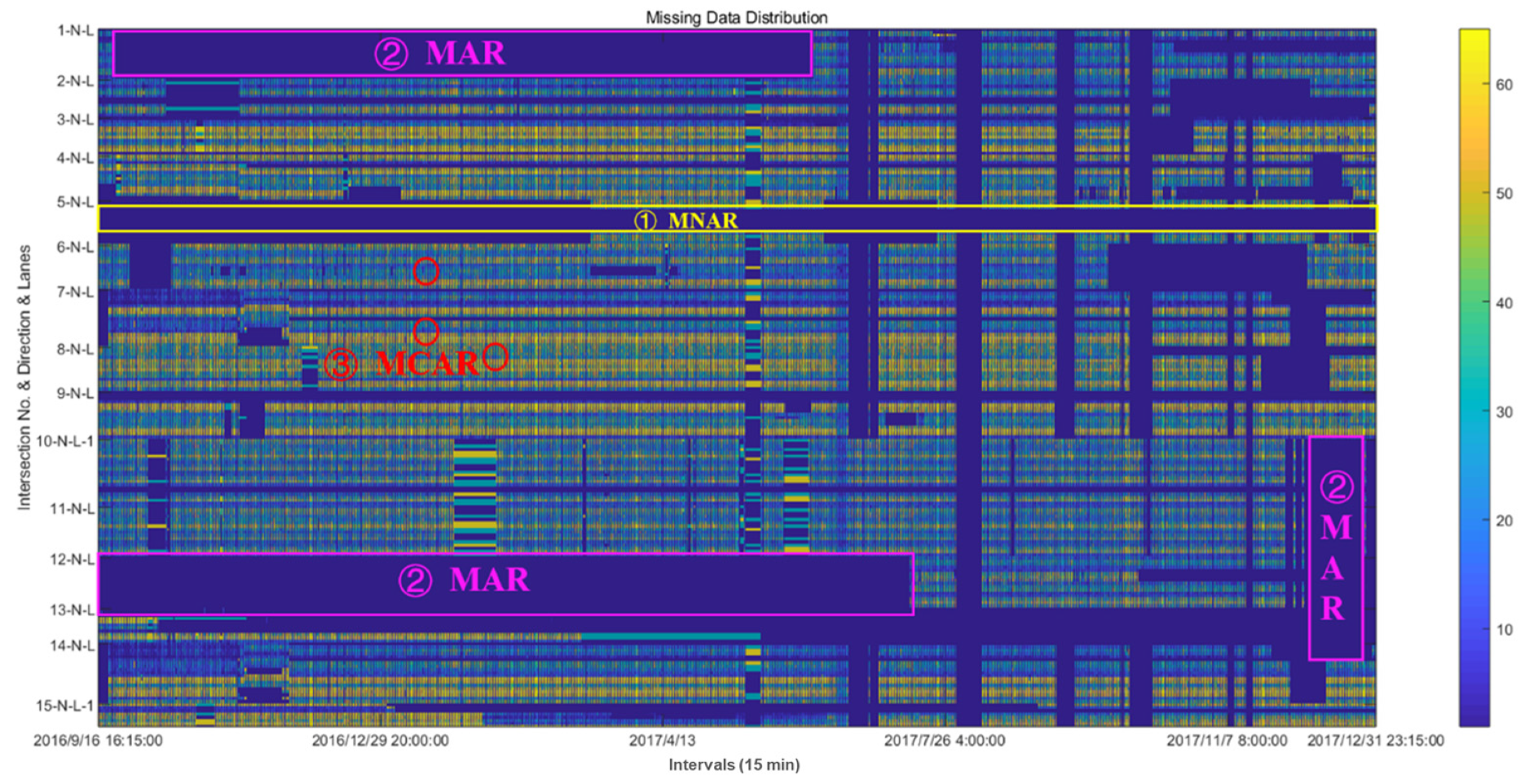
According to recent works [7,8,28,80,94], the statistical missing patterns can be divided into three types: missing at determinate/missing not at random (MNAR), missing at random (MAR), and missing completely at random (MCAR). These missing patterns are shown in Figure 1, and they have the following characteristics:

• MNAR: The missing data are regular. It usually means that there are some faults in detectors.
• MAR: The points of missing traffic data are related to nearby points. They usually occur as a group at special intervals, but the position of each group is random.
• MCAR: The missing data are isolated, random, and independent.

Actually, MCAR is a kind of MAR. MCAR is special in all MAR because the missing possibility is almost certain, and it is hard to perform the data imputation when detectors suffer from long-time malfunction. In this case, MAR and MCAR are usually used to conduct the imputation.

There is another classification measured by the length of missing time, in which the missing patterns are categorized as short-period missing values and long-period missing values [83].

2.3. Assumption

Most existing imputing methods usually make clear assumptions in advance. Because traffic variations are influenced by many factors, which cannot be fully considered, these methods are restricted when applied in many cases. The assumptions are as follows.

• Data are lost randomly.
• Missing data are at low missing rates.
• Missing data are assumed to have determined attributes or patterns.
• Missing data are mostly influenced by historical data, neighboring data, or spatial data, without consideration of variations from interval to interval, from day to day, or from upstream to downstream.

2.4. Imputation Style

There are two kinds of imputation styles: the singular choice imputation and the multiple choice imputation [6].

• Singular choice imputation (SCI)

The imputation result is directly achieved by the proposed model or scheme in SCI, in which the algorithms do not focus on multiple choices of different attributes or patterns by methods, and efforts are not taken to improve the spatiotemporal correlation analysis and do not incorporate the most valuable information for imputation. Because of the fast computational speed, SCI is often applied for real-time analysis. As most patterns and attributes are predetermined in models and strategies of prediction methods and interpolation methods, they are mostly SCI methods, such as hot deck, average, and regression.

2.

Multiple choice imputation (MCI)

MCI methods overcome the drawback of SCI methods that derive standard errors of the estimated parameters that are too small. The basic idea of MCI is: (a) proposing a model that incorporates random variation in imputing missing data; (b) generating complete datasets for M times; and (c) analyzing each complete dataset and utilizing statistical parameters, probabilistic results, and EM- or ML-iterated algorithms from M cases to infer the best single one. Thus, it can deal with the inherent uncertainty of the imputations. For MI, the data must be missing at random. Most statistical methods are MCI.

2.5. Applicable Conditions

Under various and complex traffic conditions with different data qualities, different imputation methods show distinct performances, which is related to the application and invalid conditions of the methods.

First, the relationship between imputation performance and the missing rate has been argued frequently in many studies. The effects of missing rates on hybrid neural network approaches were evaluated [95]. Each day has 12 consecutive hour gaps, which can impact on the effect of time interval and the effectiveness of selected imputation methods [64]. Gaps are generated for 10% to 90% of the dataset by using a clustering approach. It was found that the result is acceptable even with a large missing ratio [78]. Even for a challenging missing range of 1 month, the method still gives an acceptable result [61]. These methods, used to generate random gaps, are similar to the missing pattern of MNAR, in which the data loss is usually caused by some faults in the detector or in the process of communication. TDI figures out the imputation for the missing ratio up to 90% [23]. The mixed missing rate is also tested [8,93]. Consecutive interval missing data are tackled properly by the massive vector classification method, and the performance with the data of different interval units (i.e., 5 min, 15 min, and 1 h) is tested [83].

Second, the numbers of partially missing detectors and invalid detectors in the spatial range are also critical factors to be discussed, which will heavily influence MCAR and MNAR and the performance of methods affected by spatial elements. However, these kinds of studies are rare.

In summary, different methods are effective under distinct conditions, such as the number of partially missing detectors, the number of invalid detectors, interval units, missing patterns, data size, and missing rates, which can determine the real-time application performance.

• Offline imputation with moderate-to-high datasets

Many imputation works are offline since the goal of imputing data is mining the latent regulation and correlation behind the data. Without the high requirement of calculating speed, offline imputation can also fully utilize moderate-to-high datasets to capture precise patterns of traffic flows, even with data before and after the points of missing data. Since offline imputation is concentrated on imputation accuracy, the complexity of models is much higher than online imputation.

2.

Online imputation with light-to-moderate datasets

With the restriction of online calculating, the small-size input with low-dimension data is more appropriate for online imputation. With the increasing applications of real-time traffic control, traffic routing, and traffic management, the requirements of online imputation are adjusted with consideration of the balance between the calculation speed and the imputation accuracy. Some old and simple imputation methods may help a lot in this situation, with accelerations to the calculation speed.

2.6. Limitations

Based on the aforementioned characteristics of the existing imputation methods, a series of common limitations need to be resolved, which can be concluded as follow:

• Compared with the tensor-based method [23], CM [27], and KM [28], vector and matrix methods share partial spatiotemporal information so that the results seem to be good when the main features are achieved by chance. However, without sufficient information incorporated, most cases will fail, especially in extreme conditions, since daily periodicity similarity, local interval fluctuation, variation from day to day, and spatial influence between upstream and downstream should be considered.
• When data are integrated from multiple shorter-term observations, the main reason for missing data is the error at the stage of processing data. Additionally, the stage of data aggregation can lead to data loss. Moreover, the repeated and error data are considered as missing data to be imputed.
• Most methods focus on spatiotemporal feature learning, but they cannot perform very well in urban traffic. This is because being divided by signal phases and the length of the phase time of traffic lights, the turning movements can influence the variation in traffic flows both in temporal and spatial aspects [8].
• Since there is no mechanism to resolve the parameters of model structures, the parameters of model structures should be determined before the operation of imputation methods, and the chosen parameters will impact the result greatly [23,28,75].
• Probe data can be a new source that can enrich the data collected by loops and point detectors [28,84]. If the data upstream can be obtained in advance, some proper methods can be used to make the prediction or reconstruction of downstream data more accurate.
• It is worth studying the quantity of sparsity detector and location optimization with a consideration of missing data imputation under different missing rates and the relationship of their threshold conditions with the number of partially missing detectors, the number of invalid detectors, and missing rates [96].
• Although the imputation methods are various, it is vital to investigate the performance of each method under different traffic conditions and their application and invalid conditions.

2.7. Public Datasets

The benchmark datasets still need to be improved, which is a critical problem in temporal data imputation. If the benchmark datasets are lacking, the findings and methods cannot be compared well, and the proposed methods may only perform well with some special datasets. The commonly-used datasets are summarized in

Table 1. Summary of public datasets.

Dataset	City, Country	Duration	Time Resolution	Spatial Coverage	Data Type
PeMS (Li et al., 2018 [83])	California, USA	1 June 2011–31 August 2011	5 min	Three detectors in S Valley Free Way in Santa Clara, CA, USA	Traffic flow data
Communications Commission (Chen et al., 2017 [97])	Guangzhou, China	1 August 2016–30 September 2016	10 min	214 road segments in urban expressways and arterials	Traffic speed data
ANPR systems’ data (Zhang et al., 2019 [98])	China	1 December 2017–31 December 2017	30 min	Traffic management department of a city	Missing data cases
Birmingham parking data (Chen et al., 2020 [99])	Birmingham, England	4 October 2016–19 December 2016	30 min	30 car parks	14.89% missing values
Hangzhou metro passenger flow data (Chen et al., 2020 [99])	Hangzhou, China	1 October 2019–25 October 2019	10 min	80 metro stations	Incoming passenger flow
Seattle freeway traffic speed data (Chen et al., 2020 [99])	Seattle, USA	1 January 2015–28 January 2015	5 min	323 loop detectors	Freeway traffic speed data
Remote Traffic Microwave Sensors (Bae et al., 2018 [28])	Knoxville, USA	1 December 2015–	5 min	Two major highways in the Knoxville region, I-40 and I-75	Traffic count, speed, and occupancy information
Changshou Road (Chen et al., 2017 [97])	Shanghai, China	25 August 2008–29 August 2008	-	Section consists of seven signalized intersections	Travel time data
FHWA (Fard and Mohaymany [100])	Los Angeles, USA	2004–	60 min	Southern section of the US101 highway	Location, speed, acceleration, and type of vehicles
AADT (Ma et al., 2019 [96])	California, USA	2010–	-	253 road segments with 7218 data collection sites	Traffic count data
Microwave sensors (Ma et al., 2017 [27])	Beijing, China	1 June 2015–7 June 2015	2 min	Two ring expressways	Latitude and longitude, timestamp, traffic flow, speed, and occupancy
Open Data portal (Laña et al., 2018 [80])	Madrid, Spain	2014–2016	1 min	3600 ATRs in urban freeways	Resolution data

.

The PeMS dataset, built by the California Department of Transportation, is the most widely used one. The data of PeMS has been collected since 2001. The special range of data of PeMS covers the freeways across all major cities of California. The data of the PeMS dataset is collected from nearly 40,000 individual detectors. The data are aggregated for each 30 s, and the resolution of data is 5 min. The content of the PeMS dataset contains detector data, traffic counts, vehicle classification, incidents, lane closures, etc. Although the PeMS dataset has sufficient data, its environment is freeways, which means that it cannot support the data imputation studies of the urban traffic system. Microwave sensors are also an important source of data and have been distributed all over the world. The largest amount of Chinese data has been collected by the government and research institutions.

3. Missing Data Imputing Methods with Mathematical Formulation

Based on a previous literature review, we know the development of distinct massing data imputing methods. In this section, we give a brief review of their formulations.

3.1. PPCA-Based Missing Data Imputing

PPCA model assumes that every sample ${\mathrm{y}}_i$ depends on a q-dimensional latent variable $x_i$ as follows [7].

$$y_i=W{x}_i+\mu +{\epsilon }_i$$

(1)

where $d<<q$ is proposed to retrieve the common hidden feature of traffic flow data. $\mu$ is a d-dimensional column vector that characterizes the sample average of $y_i$. Here, the subscript $i$ denotes the index of the observation/latent variable. PPCA model assumes that the latent variables $x_i$ follows a q-dimensional multivariate Gaussian distribution, $x_i~N_q\left(0,I\right)$. The d-dimensional column vector ${\epsilon }_i$ is introduced as isotropic noise satisfying ${\epsilon }_i~N_d\left(0,{\sigma }^{2}I\right)$, where ${\sigma }^2$ is the scaling factor. This relaxes the strict assumption on daily flow similarity and makes the model more flexible. The projection matrix $W\in R^{d\times q}$ represents a mapping between the latent variable space and the observed variable space followed by all the observed latent variable pairs $\left(y_i,x_i\right)$.

When some elements of $y_1,\dots ,y_n$ are missing, we search $\mu$, $W$, and ${\sigma }^2$ that produce maximum likelihood in agreement with the known data

$$\arg \underset{\mu ,W,{\sigma }^2}{\max }{L}_{c1}=\arg \underset{\mu ,W,{\sigma }^2}{\max }{\displaystyle \sum _{i=1}^n\ln \left\{p\left(y_i^{miss},y_i^{known},x_i\right)\right\}}$$

(2)

where the conditional probability density function is

$$\begin{array}{ll}p\left(y_i^{miss},y_i^{known},x_i\right)& =p\left(y_i,\left.x_i\right|\mu ,W,{\sigma }^2\right)\\ & =p\left(\left.y_i\right|x_i,\mu ,W,{\sigma }^2\right)\times p\left(x_i\right)\\ & ={\left(2\pi {\sigma }^2\right)}^{-d/2}\exp \left\{-\frac{{‖y_i-W{x}_i-\mu ‖}^2}{2{\sigma }^2}\right\}\\ & \times {\left(2\pi \right)}^{-q/2}\exp \left\{-\frac{1}{2}{x}_i^T{x}_i\right\}\end{array}$$

(3)

Meanwhile, we impute $y_i^{miss}$ to best fit with the above distribution assumptions and thus the estimated maximum likelihood. Moreover, if some data are missing, $\mu$ is calculated by taking the average of the available data, and $‖\cdot ‖$ means the Euclidean norm.

3.2. GMM-Based Missing Data Imputing

The Gaussian mixture model (GMM) is commonly used for clustering. Each GMM consists of several Gaussian distributions, each of which is called a component, representing a different cluster. All the components are linearly added together to form a probability density function (PDF) of GMM.

There is a set of observed data, which is $X=\left\{x_1,\dots ,x_n\right\}$. Each vector $x_i$ is a p-dimensional vector. We assume that $X$ is generated by a GMM with $K$ components. The function $f_k\left(x_i\right)$ represents the probability density function of the $k$ component, expressing the probability of $x_i$ generated by the $k$ component. Hence, the PDF of the GMM is as follows

$$P\left(x_i\right)={\displaystyle \sum _{k=1}^K{\pi }_k{f}_k\left(x_i|{\mu }_k,{\epsilon }_k\right)}$$

(4)

where ${\pi }_k$ represents the weight of the $k$ component in the GMM, ${\mu }_k$ and ${\epsilon }_k$ represent the mean vector and covariance matrix of the $k$ component, respectively, $P\left(x_i\right)$ represents the probability of $x_i$ generated by the GMM. The PDF of the $k$ component $f_k\left(x_i|{\mu }_k,{\epsilon }_k\right)$ is expressed as

$$f_k\left(x_i|{\mu }_k,{\epsilon }_k\right)=\frac{\exp \left\{-\frac{1}{2}{\left(x_i-{\mu }_k\right)}^T{\displaystyle {\sum }_k^{-1}\left(x_i-{\mu }_k\right)}\right\}}{{\left(2\pi \right)}^{p/2}{\left|{\epsilon }_k\right|}^{1/2}}$$

(5)

In a GMM, we assume that $X$ is generated by a GMM with $k$ components and $X$. The complete data are $Y=\left(X,Z\right)=\left\{\left(x_1,z_1\right),\dots ,\left(x_n,z_n\right)\right\}$. $Z$ is the implicit category of the data. $z_i$ represents the cluster of $x_i$ and $z_i=\left(z_{i1},\dots ,z_{iK}\right)$

$$z_{ik}=\left\{\begin{array}{l}1 \mathit{if} x_i belongs to group k\\ 0 \mathit{otherwise}\end{array}\right.$$

(6)

Assuming that there are $K$ clusters and the weight of the $k$ component in the GMM is ${\pi }_k$ and ${\theta }_k$ is the corresponding parameter, the density of $z_i$ based on $x_i$ is as follows

$${\displaystyle \prod _{k=1}^K{f}_k{\left(x_i|{\theta }_k\right)}^{z_{ik}}}$$

(7)

The logarithmic likelihood function of the imputation data with some missing data of $Y$ is

$$L\left({\theta }_k,{\pi }_k,z_{ik}|x\right)={\displaystyle \sum _{i=1}^n{\displaystyle \sum _{k=1}^K{z}_{ik}\left[\log {\pi }_k{f}_k\left(x_i|{\theta }_k\right)\right]}}$$

(8)

Expectation–maximization algorithm (EM) is usually used to solve the above problem.

3.3. KNN-Based Missing Data Imputing

With the KNN method, a categorical missing value is imputed with the majority among its $k$ nearest neighbors. The average value (mean) of the $k$ nearest neighbors is regarded as the prediction for a numerical missing value. It is formally defined as follows. Given $\left(X,U,0\right)$ and the set of its $k$ nearest neighbors $D_k=\left\{\left(X_j,Y_j,1\right)|j=1,2,\dots ,k\right\}$, the KNN estimator is defined as

$$Y=\left\{\begin{array}{l}\arg {\max }_v\left\{{\displaystyle \sum _{\left(X_j,Y_j,1\right)\in D_k}1\left(Y_j=v\right)}\right\}, if \mathrm{Y} is categorical\\ \frac{1}{k}{\displaystyle \sum _{j=11}^k{Y}_j}, \mathrm{if} \mathrm{Y} is numerical\end{array}\right.$$

(9)

where $v$ is a value in the domain of the target feature $Y$ and $1\left(Y_j=v\right)$ is an indicator function that returns the value 1 if its argument is true and 0 otherwise.

Therefore, KNN imputation is a model-free method. The similarity between an instance and its nearest neighbors, determined from the differences between instances, should certainly be maximal for selecting the nearest neighbors. The usually used method is Minkowski distance (or its variants) as follows

$$d\left(i,j\right)={\displaystyle \sum _{k=1}^p{\left({\left|x_{i1}-x_{j1}\right|}^q\right)}^{1/q}}$$

(10)

where $q$ is a nonnegative integer called the Minkowski coefficient.

3.4. Copula-Based Missing Data Imputing

The copula method expresses that a joint distribution can be decomposed into a combination of several one-dimensional margin distributions and a copula function with a cumulative distribution function of marginal $F_p\left(z_p\right)$ that can be generated as follows

$$F_p\left(z_p\right)=F\left(z_1,\dots ,z_p\right)=C_{\theta }\left(F_1\left(z_1\right),\dots F_p\left(z_p\right)\right)$$

(11)

$C_{\theta }$ is a cdf of p-dimensional random variables, and is also known as a copula function. $\theta$ is a parameter vector of the copula, commonly referred to as the dependence parameter vector. The copula function can be obtained via an inversion method.

$$\left\{\begin{array}{l}{u}_i=f_i\left(z_i\right) i=1,\dots ,p\\ C\left(u_1,\dots ,u_p\right)=F_c\left(f_1^{-1}\left(u_1\right),\dots ,f_p^{-1}\left(u_p\right)\right)\end{array}\right.$$

(12)

where $u_i\in \left[0,1\right]$ represents the probability density function, $F_c\left(\cdot \right)$ is the joint distribution, and $f_i^{-1}\left(\cdot \right)$ is the inverse of the marginal distribution.

For the copula-based missing data imputing, we use the copula theory to detect the spatial correlation based on the distance, verify the spatial autocorrelation’s existence, and find the optimal correlation function. In addition, marginal distribution is also conducted to obtain an optimal distribution by the fitting process, and the parameters of the above procedure are estimated. Then, the copula-based interpolation can be finished through numerical integration of the density function to complete the missing data imputation.

3.5. Tensor-Based Missing Data Imputing

Tensor representation is one of the most practical ways to estimate a multidimensional object whose entries are indexed by several variables. Tensor is often used for extracting hidden structures and capturing underlying correlations between modes in the data with a multimode system. In many applications, tensor completion problems can formulate the missing data problem. While tensors naturally have a high dimensional characteristic, the tensor of interest is often low-rank, or approximately so. Hence, the low-rank approximation can be used for missing data estimation or tensor completion. More details can be found in the literature [75].

3.6. ARIMA-Based Missing Data Imputing

The ARIMA model is a time series analysis and prediction model and is represented by the following finite difference equations.

$$\phi \left(B\right)Y_t=\theta \left(B\right){\epsilon }_t$$

(13)

$$\phi \left(B\right)=1-{\phi }_{1}B-{\phi }_2{B}^2-\dots -{\phi }_p{B}^p$$

(14)

$$\theta \left(B\right)=1-{\theta }_{1}B-{\theta }_2{B}^2-\dots -{\theta }_q{B}^q$$

(15)

where $B{X}_t=X_{t-1}$, $B$ is the lag operator, ${\phi }_i\left(i=1,2,\dots ,p\right)$ are autoregressive parameters, ${\theta }_j\left(j=1,2,\dots q\right)$ are moving average parameters, and ${\epsilon }_t~N\left(0,{\sigma }^2\right)$ is the error term that follows a normal distribution.

The level and variance represent parameters that are analogous to cross-sectional statistical methods. The slope and autocorrelation parameters represent parameters unique to longitudinal designs. The appropriate order is used for constructing the model and forecasting time series.

3.7. Random Forest-Based Missing Data Imputing

Random forest (RF) is an algorithm that generalizes ensembles of decision trees with the ability to perform regression and classification. RF uses bagging aggregation to combine multiple random predictors to aggregate predictions by allowing for high complexity without overgeneralizing and overfitting the training data. In this approach, separate training sets are bootstrapped from the training set, and the predictive functions $\left\{\stackrel{\wedge }{f_1^{*}}\left(x\right),\stackrel{\wedge }{f_2^{*}}\left(x\right),\dots ,\stackrel{\wedge }{f_B^{*}}\left(x\right)\right\}$ are built. The final predictive part is an average of these

$${\hat{f}}_{avg}\left(x\right)=\frac{1}{B}{\displaystyle \sum _{b=1}^B\widehat{f^{*b}}\left(x\right)}$$

(16)

where the asterisk marks a function on a bootstrapped set; random forests are an improvement over bagged trees.

3.8. LSTM-Based Missing Data Imputing

To facilitate an understanding of the method in this paper, we briefly introduce the mechanism of LSTM. The advantage of LSTM is that it uses forget gates to select valuable short-term and long-term memory from the dataset and avoid the problem of vanishing and exploding gradients, rather than simply recording recurrent states by RNN. The process of LSTM is as follows

$$i_t=\sigma (W_i{x}_t+U_i{h}_{t-1}+V_i{b}_{t-1})$$

(17)

$$o_t=\sigma (W_o{x}_t+U_o{h}_{t-1}+V_o{b}_{t-1})$$

(18)

$${\tilde{C}}_t=tanh(W_C{x}_t+U_C{h}_{t-1}+V_C{b}_{t-1})$$

(19)

$$C_t={\psi }_t{C}_{t-1}+i_t{\tilde{C}}_t$$

(20)

$$h_t=o_{t}tanh(C_t)$$

(21)

Equations (17)–(19) refer to the input gate($i_t$), forget gate(${\psi }_t$), and output gate($o_t$), respectively, in which $W$, $U$, and $V$ are trainable weighted transition matrices governing the connection from corresponding inputs to the hidden layer, while $b$ is bias terms, $x_t$ is the input information at the interval $t$, $h_{t-1}$ is the output of the hidden layer at the interval $t-1$, and $C_{t-1}$ is the cell information at the interval $t-1$; ${\tilde{C}}_t$ and $C_t$ are the candidate and new cell information at the interval $t$, respectively.

LSTM-M is used for managing missing data from the two categories, in which a long-period and a short-period mechanism are designed for modeling missing data in the input variables, and hidden states are employed to capture the properties mentioned above. Weights $r_t$ are introduced to control the impact of a unique meaning and time stamp and to be flexible from 0 to 1 according to the time interval relative to the previous variables. Thus, the weights should represent the patterns and be conducive to the inference tasks

$$r_t=\exp \left\{-\max \left(0,W_r{l}_t+b_r\right)\right\}$$

(22)

where $W_r$ and $b_r$ are parameters to be learned jointly with those in the LSTM network. The LSTM-M time series model for missing data incorporates two temporal prediction scales to obtain the missing data directly from the input values.

4. Test and Results

4.1. Test Data

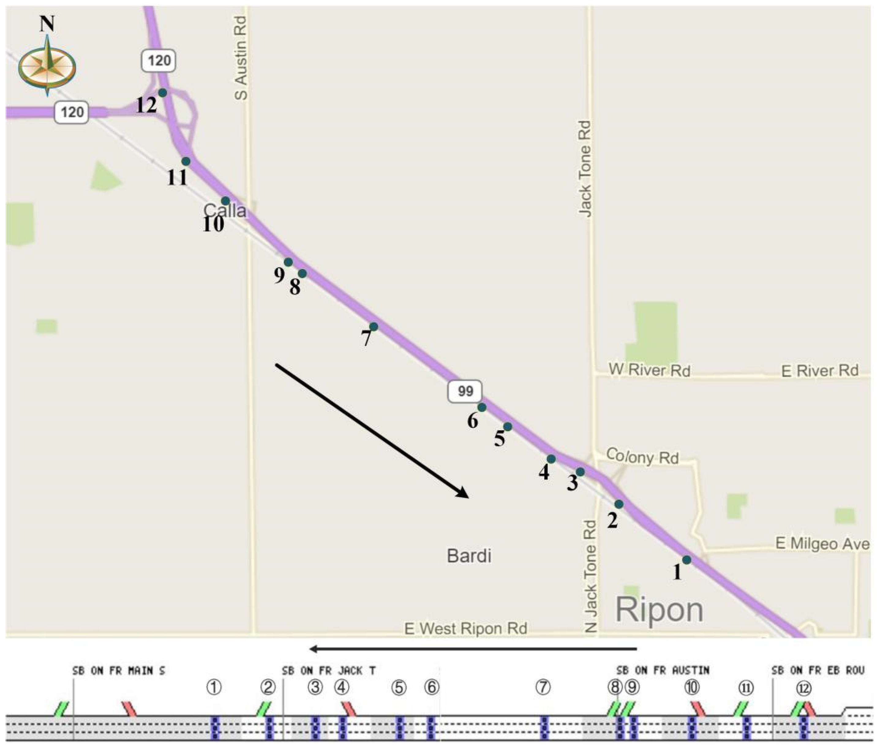
This paper uses PeMS to conduct the test. The data of PeMS were collected from the highways in California. This paper selects several adjacent stations. There are 12 loop detectors, and they are located on the southbound Highway 99. Figure 2 summarizes the selected 12 detectors of the PeMS dataset. The data from 1 January 2018 to 31 December 2019 are used to do the test. Detector IDs, detector locations, and the direction are shown in

Table 2. Description of 12 detectors’ corresponding information.

Detector ID	Location	Direction
1	241.59	North to South
2	241.20	North to South
3	240.83	North to South
4	240.43	North to South
5	240.34	North to South
6	239.82	North to South
7	238.97	North to South
8	238.76	North to South
9	238.37	North to South
10	238.18	North to South
11	237.87	North to South
12	235.50	North to South

.

4.2. Test and Results

Normalized mean absolute error (NMAE) and normalized root mean square error (NRMSE) are used to evaluate the performance of the imputation methods. The formulations for calculating NMAE and NRMSE are as follows

$$NMAE=\frac{{\displaystyle {\sum }_{i,j}|f_{ij}-\stackrel{\wedge }{f_{ij}}|}}{{\displaystyle {\sum }_{i,j}\left|f_{ij}\right|}}$$

(23)

$$NRMSE=\frac{\sqrt{\frac{1}{\left|\varphi \right|}{{\displaystyle {\sum }_{i,j}|f_{ij}-\stackrel{\wedge }{f_{ij}}|}}^2}}{\frac{1}{T}{\displaystyle {\sum }_{i,j}\left|f_{ij}\right|}}$$

(24)

where $\varphi$ is a normalized parameter.

Then, all mentioned methods are tested with integrated data missing patterns. The respective results are shown in

Table 3. Results with integrated data missing patterns.

Missing Ratio		10%	20%	30%	40%	50%	60%	70%	80%	90%
PPCA	NRMSE	14.76	12.17	13.61	13.62	14.09	17.27	22.00	22.96	24.67
	NMAE	9.41	8.18	8.54	8.96	9.85	13.31	17.65	18.39	19.81
GMM	NRMSE	30.61	31.06	36.13	48.46	50.91	53.21	55.23	59.06	62.17
	NMAE	22.35	24.79	29.13	40.52	41.66	44.41	46.29	54.16	58.12
KNN	NRMSE	16.62	15.09	16.93	18.06	20.81	16.52	16.94	30.19	33.13
	NMAE	10.07	9.23	10.22	10.47	13.09	10.68	10.74	20.96	24.13
Copula	NRMSE	32.31	29.05	34.18	33.83	34.32	31.07	33.47	34.13	34.14
	NMAE	24.23	22.39	25.93	25.67	26.28	24.02	25.05	25.88	25.95
Tensor	NRMSE	18.69	12.90	18.09	23.37	28.22	14.59	15.92	27.09	29.26
	NMAE	10.79	8.34	10.13	12.82	17.03	9.67	9.70	19.76	22.07
ARIMA	NRMSE	28.81	23.25	27.95	26.67	28.04	25.76	26.66	27.44	27.81
	NMAE	22.07	19.10	22.15	21.55	22.32	20.08	20.46	21.55	22.13
Random Forest	NRMSE	30.61	33.43	36.78	41.11	41.62	39.98	40.82	43.13	46.91
	NMAE	22.35	25.18	32.73	31.08	32.06	31.22	30.70	34.22	38.12
LSTM	NRMSE	12.40	14.80	20.03	28.43	33.53	37.36	40.68	41.86	43.12
	NMAE	8.06	9.69	15.18	20.32	24.36	28.51	30.68	31.72	33.10
LSTM-M	NRMSE	11.92	15.26	19.37	28.61	32.59	38.15	40.01	41.29	42.33
	NMAE	7.54	10.02	14.24	19.97	23.46	29.21	30.27	31.06	32.13

. PPCA has the best performance.

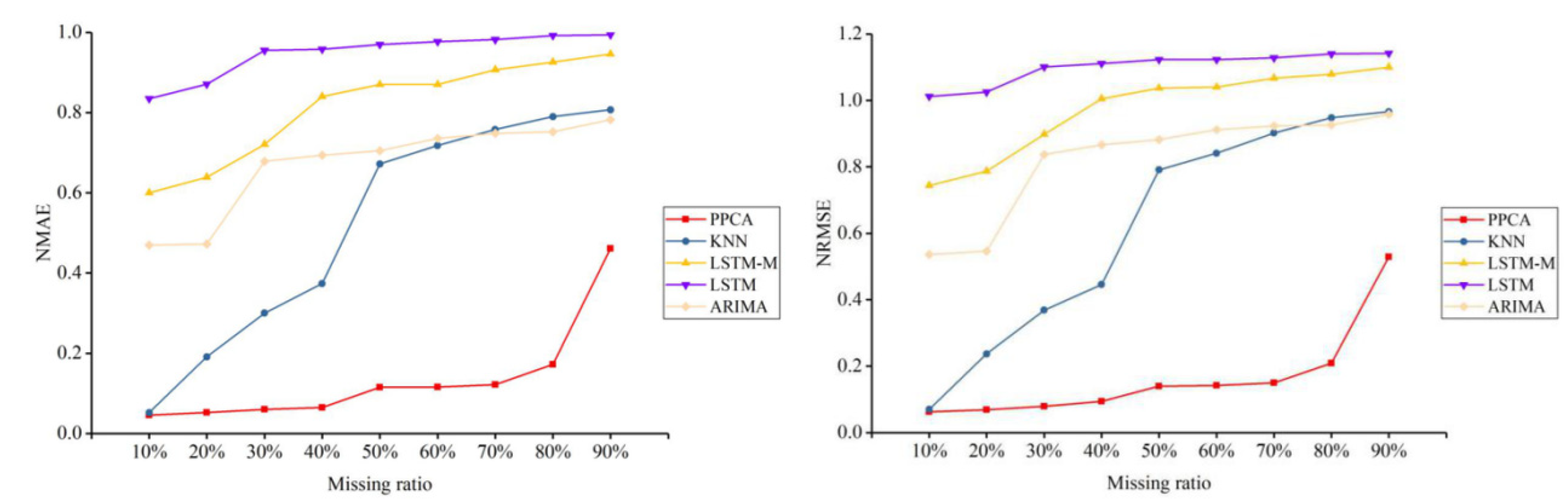
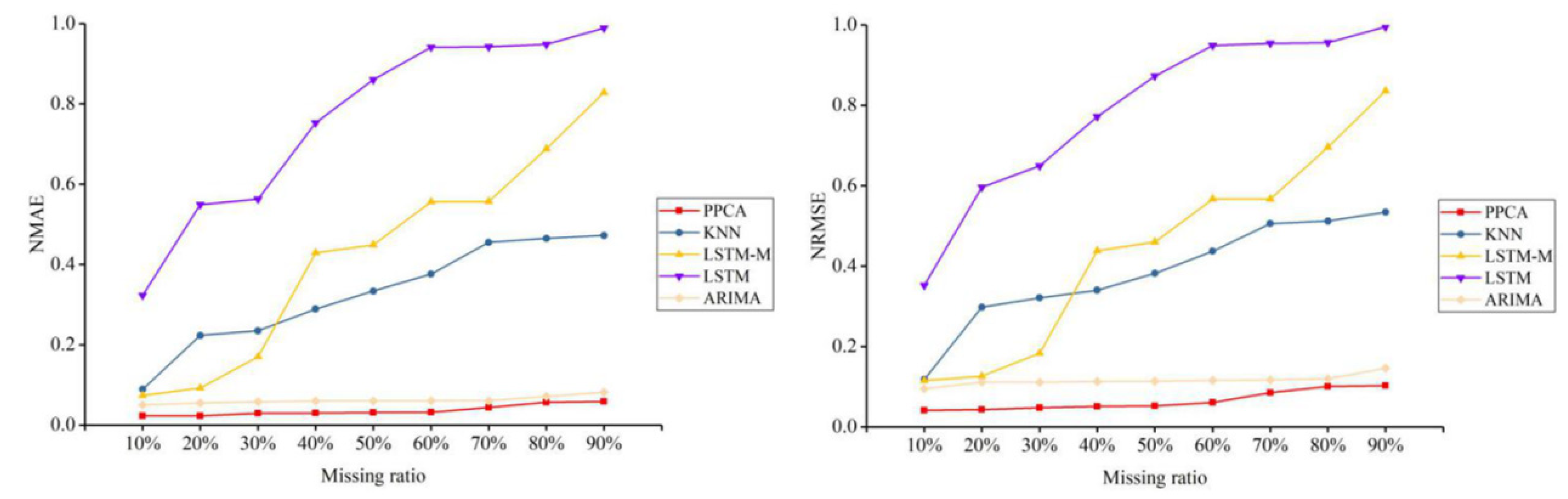
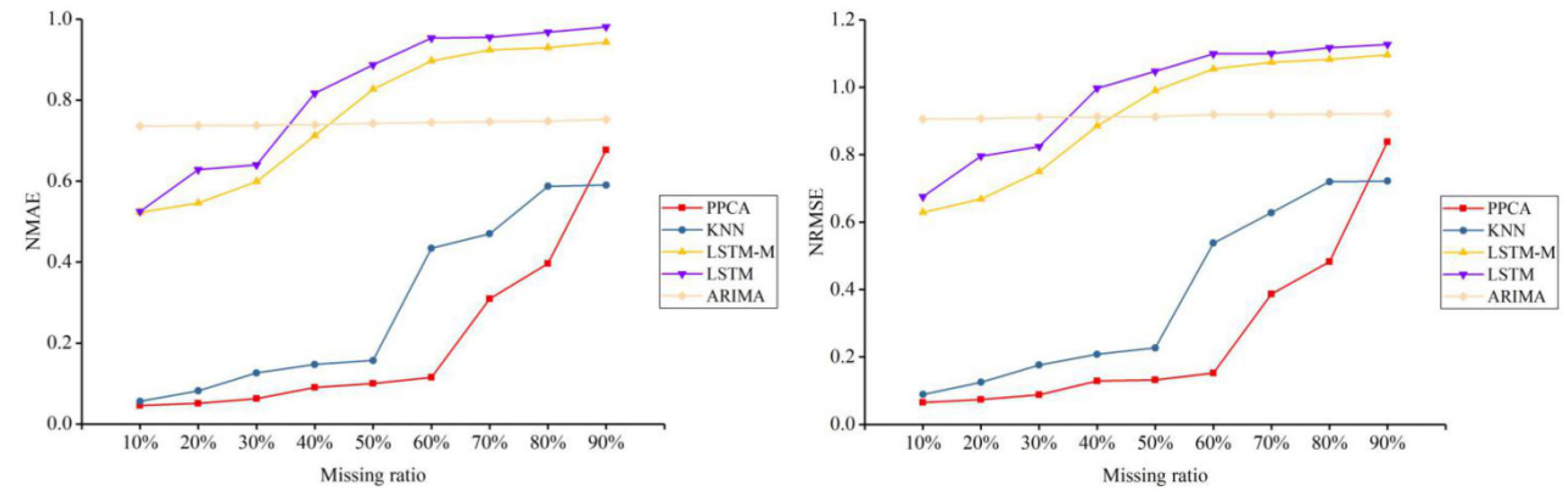
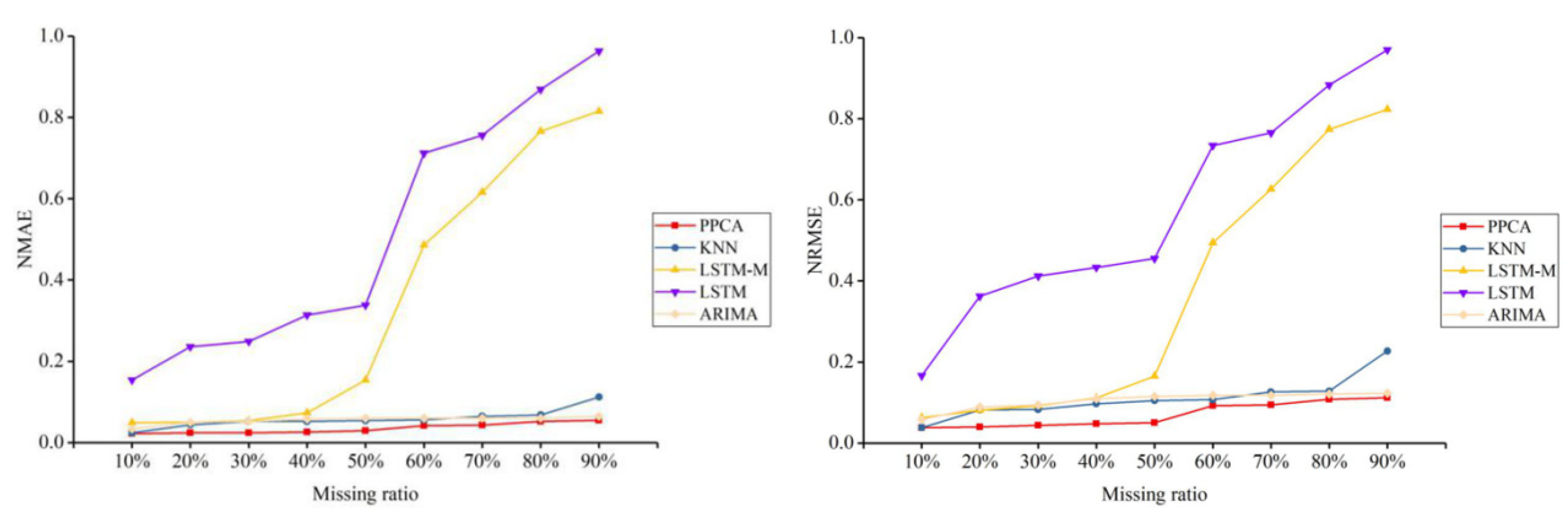
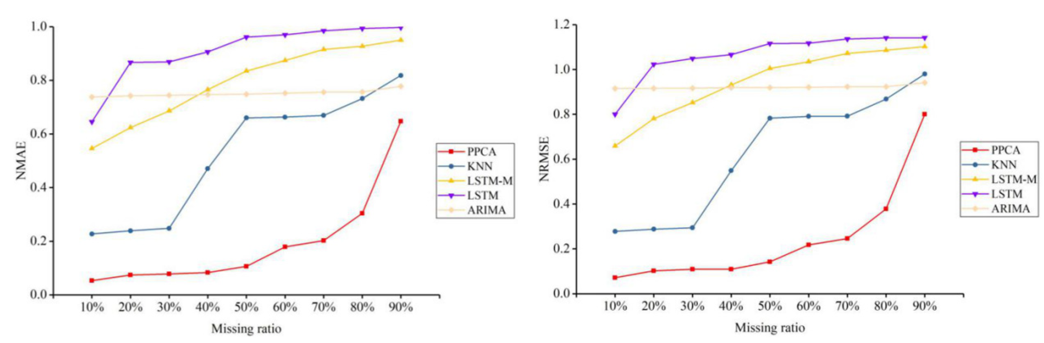
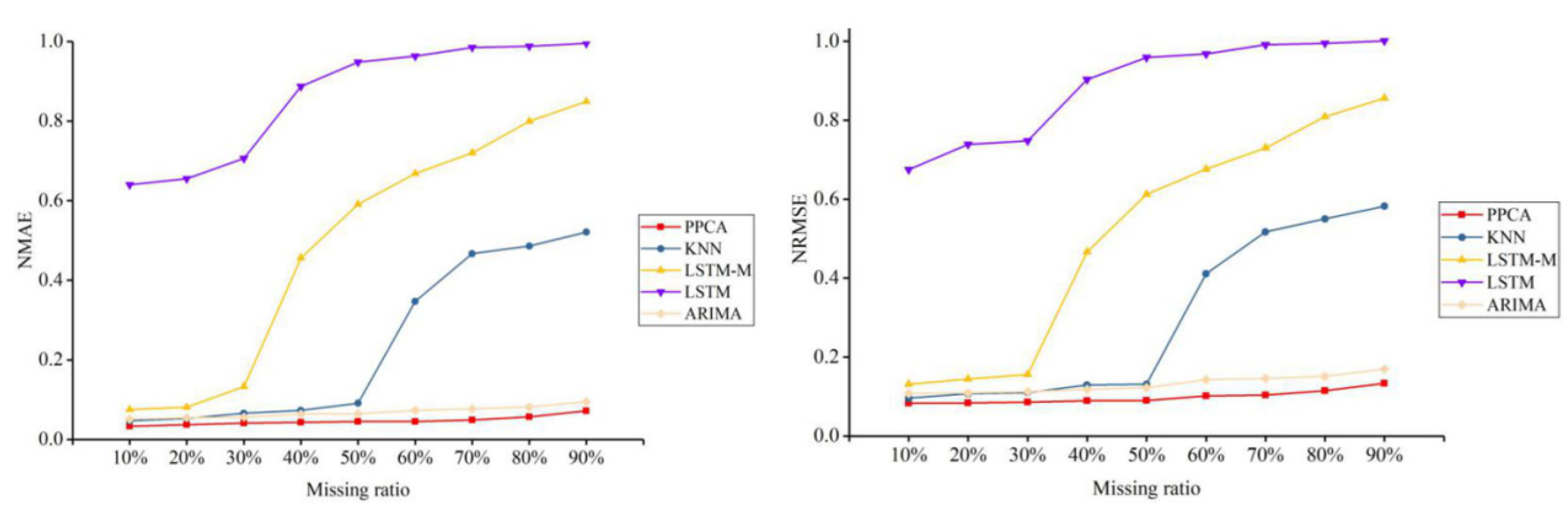
For a better test, five representative methods of all types of methods are selected to conduct further tests and comparisons, including PPCA, KNN, LSTM, LSTM-M, and ARIMA, and they are tested under three different missing patterns (MCAR, MAR, and MNAR) and missing ratios. The results are shown in Figure 3, Figure 4, Figure 5, Figure 6, Figure 7 and Figure 8.

For the traffic flow data depicted in Figure 3, Figure 5, and Figure 7, PPCA is clearly superior to the other methods. In the MAR scenario, KNN also shows a good imputation advantage. Under different missing ratios, the performance of ARIMA is relatively flat. The other four temporal imputation methods change continuously with the missing ratio. In the traffic speed data depicted in Figure 4, Figure 6, and Figure 8, PPCA significantly outperforms the other methods, and ARIMA has amazing performance. It can be seen that for different data situations, different temporal imputation methods perform in various ways. Compared with the other three methods, the fluctuations of PPCA and ARIMA are relatively small. In terms of traffic speed in the MAR scenario, KNN shows a good imputation advantage. It can be seen that KNN performs significantly better than other methods except for PPCA in MAR scenarios. Although the improved LSTM-M is better than LSTM for errors of both different flow and speed datasets, LSTM-M and LSTM are worse than the other methods.

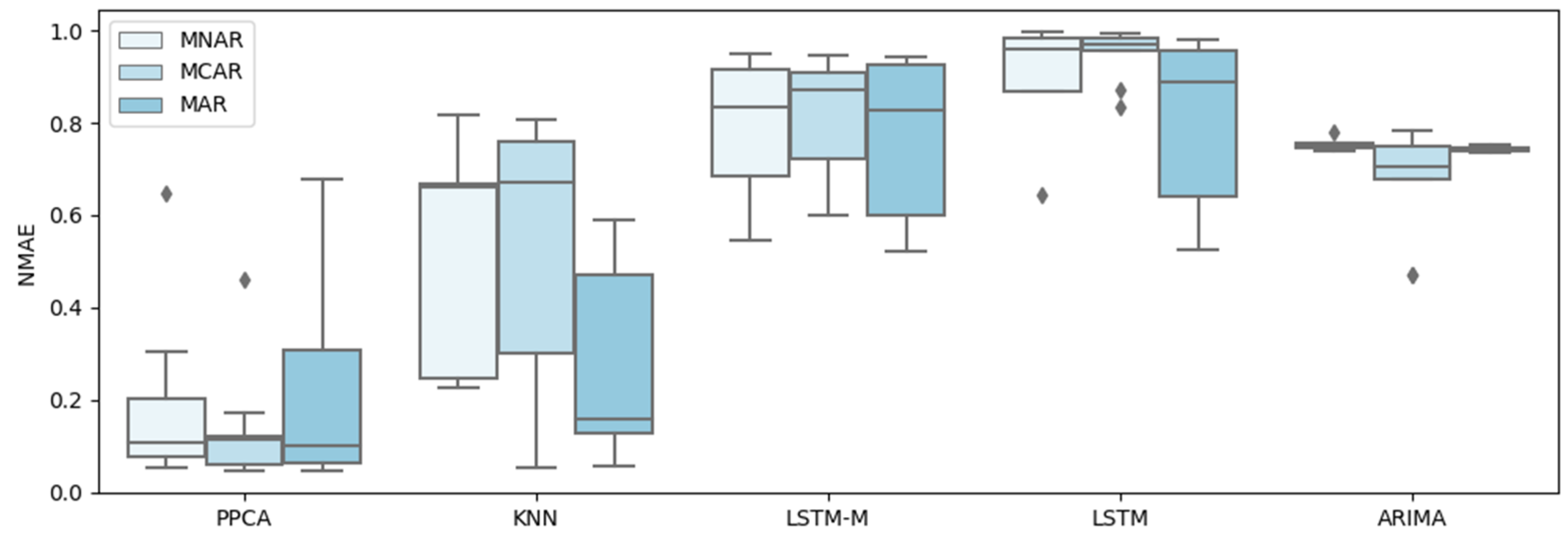
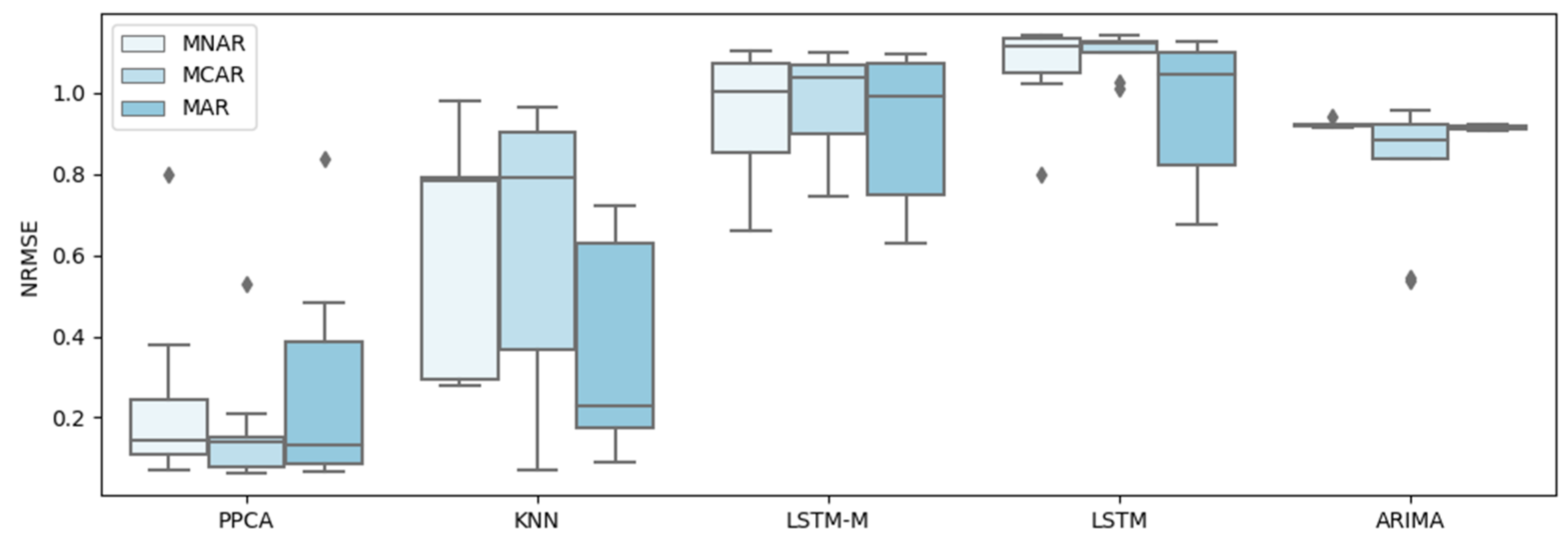
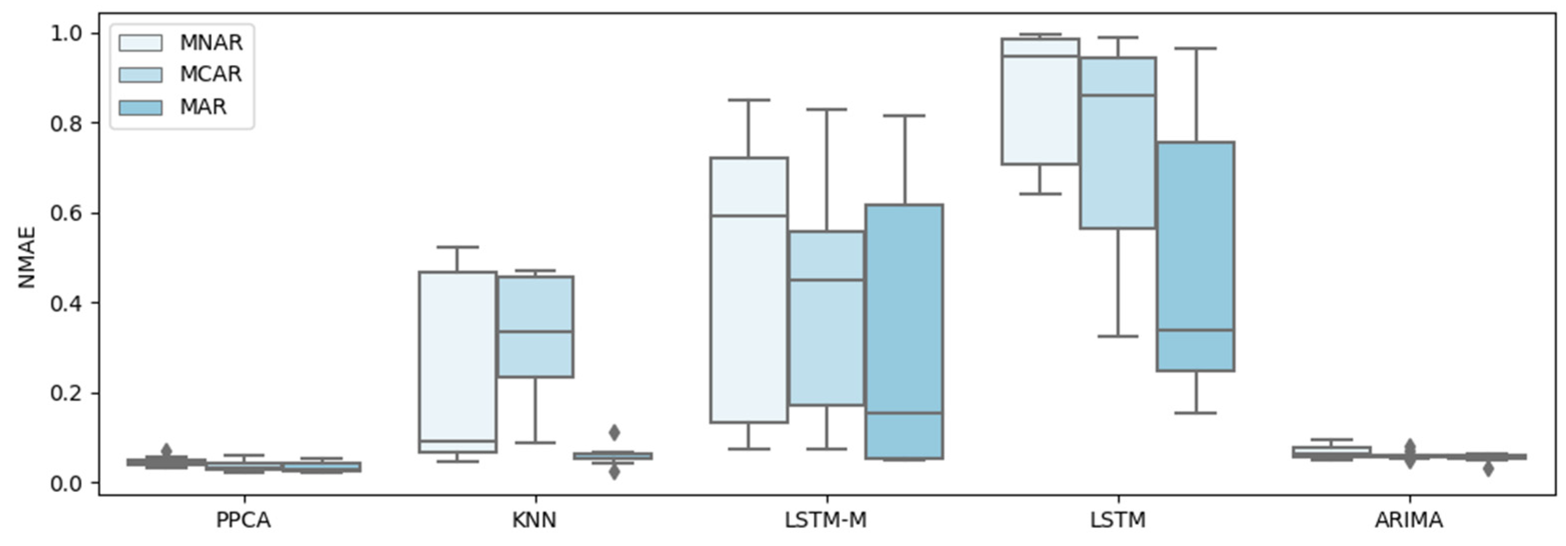
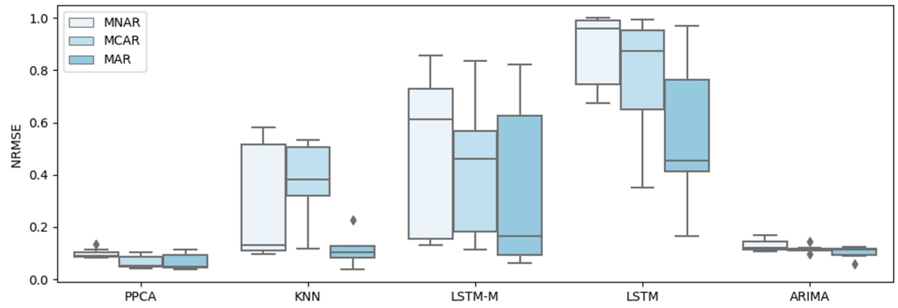
A similar conclusion can be obtained by inspecting Figure 9, Figure 10, Figure 11 and Figure 12, which show the errors for the different methods of three missing patterns. Figure 9 and Figure 10 show boxplots for the average flow imputation results of different missing ratios. Figure 11 and Figure 12 show boxplots for the average speed imputation results of different missing ratios. These figures display different missing patterns clearly. The input performance of each method is different. In terms of the temporal data imputation of traffic flow, PPCA is far superior to other methods, followed by KNN. Traditional LSTM and the improved LSTM-M are not effective.

In the temporal data imputation of traffic speed, PPCA is far superior to other methods. Surprisingly, ARIMA shows unexpected results, far better than KNN, LSTM, and LSTM-M.

5. Discussion

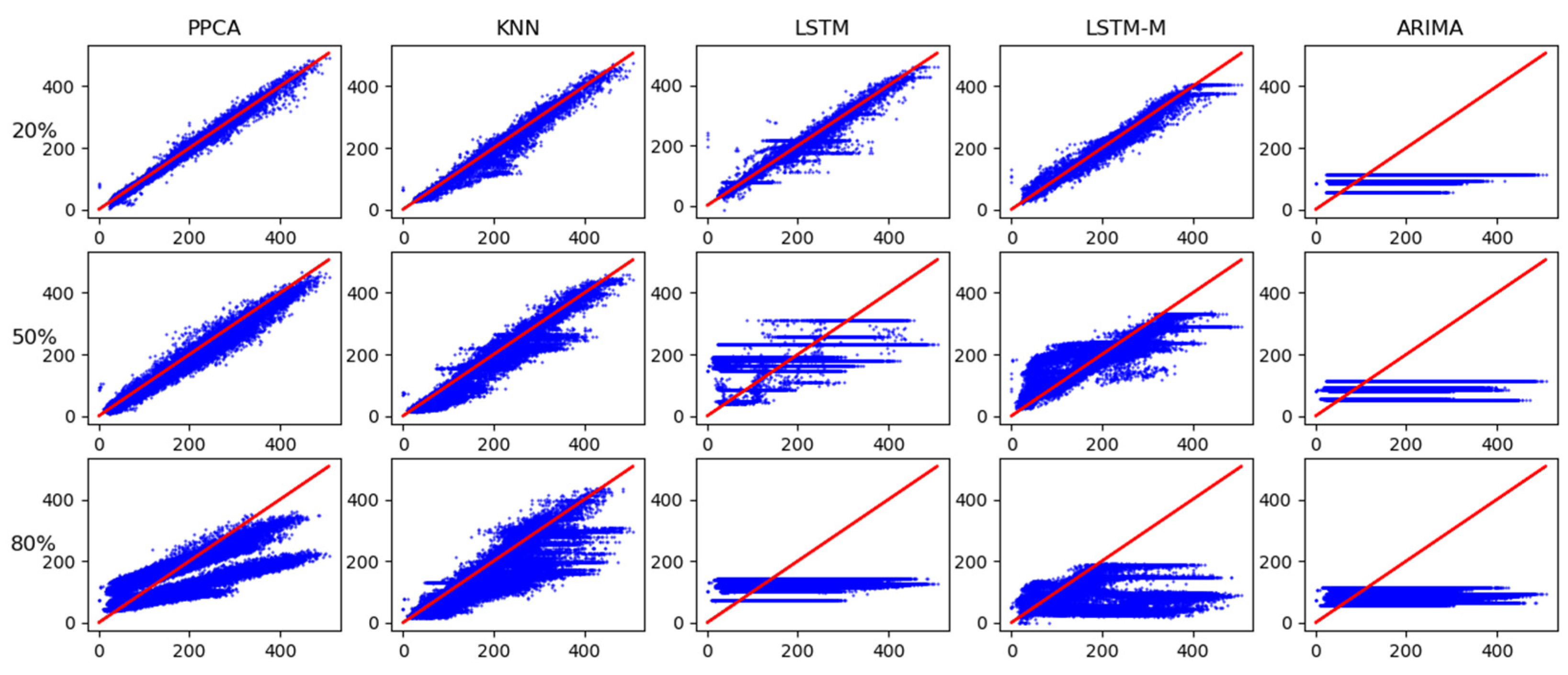
In actual traffic conditions, three missing patterns are often randomly integrated. We verify the random missing patterns by different methods. As shown in Figure 13 for the missing flow of 20%, 50%, and 80%, the correspondence relationship between the ground truth (abscissa) and the imputation value (ordinate) clearly shows that the closer to the red line, the more accurate the imputation value is compared to the ground truth. PPCA performs the best among the five temporal imputation methods. As the missing ratio increases, all models show gradual fragility, which is moving away from the red line.

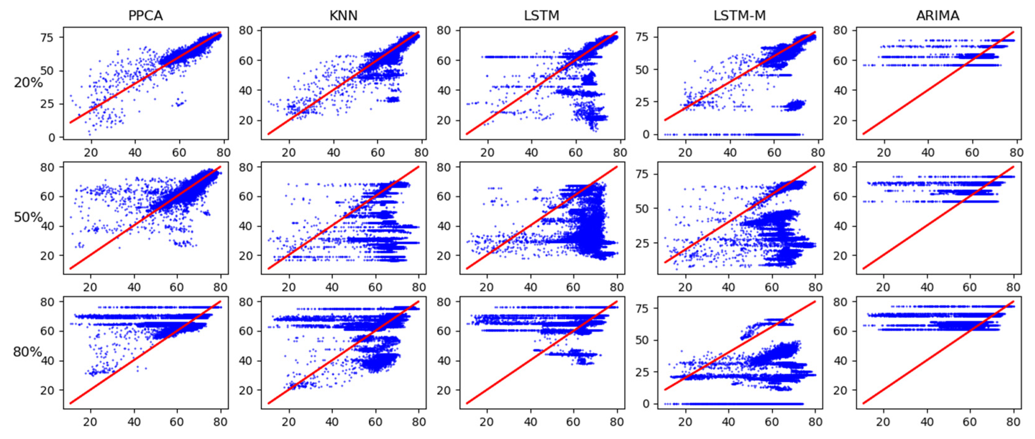
As shown in Figure 14 for missing speeds of 20%, 50%, and 80%, in the five temporal imputation models, we can still clearly see that the corresponding relationship between the ground truth (abscissa) of PPCA and the imputation value (ordinate) is closer to the middle red line. With the increase in the missing ratio, the temporal imputation methods show gradual fragility of a different degree.

6. Conclusions

Missing values of traffic time series data is a common problem in intelligent transportation systems. This paper reviews the development of temporal imputation. It summarizes the strategy of temporal imputation, covering all stages of the process, from creating data sets with artificial blanks to evaluating the obtained results. We have witnessed major developments in transportation imputation research. Five representative methods are compared, which are widely used: PPCA, KNN, LSTM, LSTM-M, and ARIMA. Models capture important temporal information in the datasets from different patterns to estimate missing values. All missing patterns show different degrees and provide reliable results with different missing rates. The complex upstream–downstream correlations in urban road networks also need more explanation. We will discuss the summary of spatial imputation and spatial–temporal imputation models in future work.

References

- You, L.; Tunçer, B.; Zhu, R.; Xing, H.; Yuen, C. A Synergetic Orchestration of Objects, Data, and Services to Enable Smart Cities. IEEE Internet Things J. 2019, 6, 10496–10507. [Google Scholar] [CrossRef]
- You, L.; Zhao, F.; Cheah, L.; Jeong, K.; Zegras, P.C.; Ben-Akiva, M. A Generic Future Mobility Sensing System for Travel Data Collection, Management, Fusion, and Visualization. IEEE Trans. Intell. Transp. Syst. 2019, 21, 4149–4160. [Google Scholar] [CrossRef]
- Sun, B.; Jiao, P. Spatio-temporal segmented traffic flow prediction with ANPRS data based on improved XGBoost. J. Adv. Transp. 2021, 2021, 5559562. [Google Scholar] [CrossRef]
- You, L.; Tuncer, B.; Xing, H. Harnessing multi-source data about public sentiments and activities for informed design. IEEE Trans. Knowl. Data Eng. 2018, 31, 343–356. [Google Scholar] [CrossRef]
- Turner, S.; Albert, L.; Gajewski, B.; Eisele, W. Archived intelligent transportation system data quality: Preliminary analyses of San Antonio TransGuide data. Transp. Res. Rec. 2000, 1719, 77–84. [Google Scholar] [CrossRef]
- Conklin, J.H.; Smith, B.L. The use of local lane distribution patterns for the estimation of missing data in transportation management systems. Transp. Res. Rec. 2002, 1811, 50–56. [Google Scholar]
- Van Buuren, S. Flexible Imputation of Missing Data; Chapman and Hall/CRC: Boca Raton, FL, USA, 2018. [Google Scholar]
- Qu, L.; Li, L.; Zhang, Y.; Hu, J. PPCA-based missing data imputation for traffic flow volume: A systematical approach. IEEE Trans. Intell. Transp. Syst. 2009, 10, 512–522. [Google Scholar]
- Vlahogianni, E.I.; Golias, J.C.; Karlaftis, M.G. Short-term traffic forecasting: Overview of objectives and methods. Transp. Rev. 2004, 24, 533–557. [Google Scholar] [CrossRef]
- Van Lint, J.W.C.; Hoogendoorn, S.P.; Van Zuylen, H.J. Accurate freeway travel time prediction with state-space neural networks under missing data. Transp. Res. Part C Emerg. Technol. 2005, 13, 347–369. [Google Scholar] [CrossRef]
- Zhang, J.; Wang, F.Y.; Wang, K.; Lin, W.; Xu, X.; Chen, C. Data-driven intelligent transportation systems: A survey. IEEE Trans. Intell. Transp. Syst. 2011, 12, 1624–1639. [Google Scholar] [CrossRef]
- Chen, C.; Wang, Y.; Li, L.; Hu, J.; Zhang, Z. The retrieval of intra-day trend and its influence on traffic prediction. Transp. Res. Part C Emerg. Technol. 2012, 22, 103–118. [Google Scholar] [CrossRef]
- You, L.; He, J.; Wang, W.; Cai, M. Autonomous Transportation Systems and Services Enabled by the Next-Generation Network. IEEE Netw. 2022, 3, 66–72. [Google Scholar] [CrossRef]
- Kim, J.O.; Curry, J. The treatment of missing data in multivariate analysis. Sociol. Methods Res. 1977, 6, 215–240. [Google Scholar] [CrossRef]
- Raaijmakers, Q.A.W. Effectiveness of different missing data treatments in surveys with Likert-type data: Introducing the relative mean substitution approach. Educ. Psychol. Meas. 1999, 59, 725–748. [Google Scholar] [CrossRef]
- Grzymala-Busse, J.W.; Hu, M. A comparison of several approaches to missing attribute values in data mining. In Proceedings of the International Conference on Rough Sets and Current Trends in Computing, Banff, AB, Canada, 16–19 October 2000; Springer: Berlin/Heidelberg, Germany, 2000; pp. 378–385. [Google Scholar]
- Chen, J.; Shao, J. Nearest neighbor imputation for survey data. J. Off. Stat. 2000, 16, 113–131. [Google Scholar]
- Nguyen, L.N.; Scherer, W.T. Imputation Techniques to Account for Missing Data in Support of Intelligent Transportation Systems Applications; Center for Transportation Studies, University of Virginia: Charlottesville, VA, USA, 2003. [Google Scholar]
- Gold, D.L.; Turner, S.M.; Gajewski, B.J.; Spiegelman, C. Imputing missing values in its data archives for intervals under 5 minutes. In Proceedings of the Transportation Research Board 80th Annual Meeting, Washington, DC, USA, 7–11 January 2001. [Google Scholar]
- Zhong, M.; Lingras, P.; Sharma, S. Estimation of missing traffic counts using factor, genetic, neural, and regression techniques. Transp. Res. Part C Emerg. Technol. 2004, 12, 139–166. [Google Scholar] [CrossRef]
- Sun, B.; Sun, T.; Zhang, Y.; Jiao, P. Urban traffic flow online prediction based on multi-component attention mechanism. IET Intell. Transp. Syst. 2020, 14, 1249–1258. [Google Scholar] [CrossRef]
- Zhang, Y.; Liu, Y. Data imputation using least squares support vector machines in urban arterial streets. IEEE Signal Processing Lett. 2009, 16, 414–417. [Google Scholar] [CrossRef]
- Tan, H.; Feng, G.; Feng, J.; Wang, W.; Zhang, Y.J.; Li, F. A tensor-based method for missing traffic data completion. Transp. Res. Part C Emerg. Technol. 2013, 28, 15–27. [Google Scholar] [CrossRef] [Green Version]
- Tang, J.; Zhang, G.; Wang, Y.; Wang, H.; Liu, F. A hybrid approach to integrate fuzzy C-means based imputation method with genetic algorithm for missing traffic volume data estimation. Transp. Res. Part C Emerg. Technol. 2015, 51, 29–40. [Google Scholar] [CrossRef]
- Tan, H.; Wu, Y.; Shen, B.; Jin, P.J.; Ran, B. Short-term traffic prediction based on dynamic tensor completion. IEEE Trans. Intell. Transp. Syst. 2016, 17, 2123–2133. [Google Scholar] [CrossRef]
- Duan, Y.; Lv, Y.; Liu, Y.L.; Wang, F.Y. An efficient realization of deep learning for traffic data imputation. Transp. Res. Part C Emerg. Technol. 2016, 72, 168–181. [Google Scholar] [CrossRef]
- Ma, X.; Luan, S.; Du, B.; Yu, B. Spatial copula model for imputing traffic flow data from remote microwave sensors. Sensors 2017, 17, 2160. [Google Scholar] [CrossRef] [PubMed] [Green Version]
- Bae, B.; Kim, H.; Lim, H.; Liu, Y.; Han, L.D.; Freeze, P.B. Missing data imputation for traffic flow speed using spatio-temporal cokriging. Transp. Res. Part C Emerg. Technol. 2018, 88, 124–139. [Google Scholar] [CrossRef]
- Rubin, D.B. Inference and missing data. Biometrika 1976, 63, 581–592. [Google Scholar] [CrossRef]
- Smith, B.L.; Scherer, W.T.; Conklin, J.H. Exploring Imputation Techniques for Missing Data in Transportation Management Systems. Transp. Res. Rec. 2003, 1836, 132–142. [Google Scholar] [CrossRef]
- Dailey, D.J. Improved Error Detection for Inductive Loop Sensors; Transportation Research Board: Washington, DC, USA, 1993. [Google Scholar]
- Nihan, N.L. Aid to determining freeway metering rates and detecting loop errors. J. Transp. Eng. 1997, 123, 454–458. [Google Scholar] [CrossRef]
- Ghosh, B.; Basu, B.; O’Mahony, M.M. Time-series modelling for forecasting vehicular traffic flow in Dublin. In Proceedings of the 84th Annual Meeting of the Transportation Research Board, Washington, DC, USA, 9–13 January 2005. [Google Scholar]
- Zhong, M.; Sharma, S.; Liu, Z. Assessing robustness of imputation models based on data from different jurisdictions: Examples of Alberta and Saskatchewan, Canada. Transp. Res. Rec. 2005, 1917, 116–126. [Google Scholar] [CrossRef]
- Vlahogianni, E.I.; Karlaftis, M.G.; Golias, J.C. Optimized and meta-optimized neural networks for short-term traffic flow prediction: A genetic approach. Transp. Res. Part C Emerg. Technol. 2005, 13, 211–234. [Google Scholar] [CrossRef]
- Contreras-Reyes, J.E. Rényi entropy and divergence for VARFIMA processes based on characteristic and impulse response functions. Chaos Solitons Fractals 2022, 160, 112268. [Google Scholar] [CrossRef]
- Van Der Voort, M.; Dougherty, M.; Watson, S. Combining Kohonen maps with ARIMA time series models to forecast traffic flow. Transp. Res. Part C Emerg. Technol. 1996, 4, 307–318. [Google Scholar] [CrossRef] [Green Version]
- Williams, B.M. Multivariate vehicular traffic flow prediction: Evaluation of ARIMAX modeling. Transp. Res. Rec. 2001, 1776, 194–200. [Google Scholar] [CrossRef]
- Kamarianakis, Y.; Prastacos, P. Forecasting traffic flow conditions in an urban network: Comparison of multivariate and univariate approaches. Transp. Res. Rec. 2003, 1857, 74–84. [Google Scholar] [CrossRef]
- Min, X.; Hu, J.; Zhang, Z. Urban traffic network modeling and short-term traffic flow forecasting based on GSTARIMA model. In Proceedings of the 13th International IEEE Conference on Intelligent Transportation Systems, Funchal, Portugal, 19–22 September 2010; IEEE: New York City, NY, USA, 2010; pp. 1535–1540. [Google Scholar]
- Min, W.; Wynter, L. Real-time road traffic prediction with spatiotemporal correlations. Transp. Res. Part C Emerg. Technol. 2011, 19, 606–616. [Google Scholar] [CrossRef]
- Stathopoulos, A.; Karlaftis, M.G. A multivariate state space approach for urban traffic flow modeling and prediction. Transp. Res. Part C Emerg. Technol. 2003, 11, 121–135. [Google Scholar] [CrossRef]
- Gazis, D.; Liu, C. Kalman filtering estimation of traffic counts for two network links in tandem. Transp. Res. Part B Methodol. 2003, 37, 737–745. [Google Scholar] [CrossRef]
- Ni, D.; Leonard, J.D. Markov chain monte carlo multiple imputation using bayesian networks for incomplete intelligent transportation systems data. Transp. Res. Rec. 2005, 1935, 57–67. [Google Scholar] [CrossRef]
- Sun, S.; Yu, G.; Zhang, C. Short-term traffic flow forecasting using sampling Markov Chain method with incomplete data. In IEEE Intelligent Vehicles Symposium; IEEE: Piscataway, NJ, USA, 2004; pp. 437–441. [Google Scholar]
- Sun, S.; Zhang, C.; Yu, G. A Bayesian network approach to traffic flow forecasting. IEEE Trans. Intell. Transp. Syst. 2006, 7, 124–132. [Google Scholar] [CrossRef]
- Kamarianakis, Y.; Shen, W.; Wynter, L. Real-time road traffic forecasting using regime-switching space-time models and adaptive LASSO. Appl. Stoch. Models Bus. Ind. 2012, 28, 297–315. [Google Scholar] [CrossRef]
- Sun, S.; Huang, R.; Gao, Y. Network-scale traffic modeling and forecasting with graphical lasso and neural networks. J. Transp. Eng. 2012, 138, 1358–1367. [Google Scholar] [CrossRef] [Green Version]
- Allison, P.D. Missing Data; Sage Publications: Thousand Oaks, CA, USA, 2001. [Google Scholar]
- Holt, C.C. Forecasting seasonals and trends by exponentially weighted moving averages. Int. J. Forecast. 2004, 20, 5–10. [Google Scholar] [CrossRef]
- De Boor, C. A Practical Guide to Splines; Springer: New York, NY, USA, 1978. [Google Scholar]
- Acurna, E.; Rodriguez, C. The treatment of missing values and its effect in the classifier accuracy, classification, clustering, and data mining applications. In Proceedings of the Meeting of the International Federation of Classification Societies (IFCS), Chicago, IL, USA, 15–18 July 2004; Springer: Berlin/Heidelberg, Germany, 2004; pp. 639–647. [Google Scholar]
- Liu, P.; Lei, L.; Zhang, X.F. A comparison study of missing value processing methods. Comput. Sci. 2004, 31, 155–156. [Google Scholar]
- Chen, C.; Kwon, J.; Rice, J.; Skabardonis, A.; Varaiya, P. Detecting errors and imputing missing data for single-loop surveillance systems. Transp. Res. Rec. 2003, 1855, 160–167. [Google Scholar] [CrossRef]
- Al-Deek, H.M.; Venkata, C.; Chandra, S.R. New algorithms for filtering and imputation of real-time and archived dual-loop detector data in I-4 data warehouse. Transp. Res. Rec. 2004, 1867, 116–126. [Google Scholar] [CrossRef]
- Kim, H.; Lovell, D.J. Traffic information imputation using a linear model in vehicular ad hoc networks. In Proceedings of the 2006 IEEE Intelligent Transportation Systems Conference, Toronto, ON, Canada, 17–20 September 2006; pp. 1406–1411. [Google Scholar]
- Boyles, S. Comparison of Interpolation Methods for Missing Traffic Volume Data; Transportation Research Board: Washington, DC, USA, 2011. [Google Scholar]
- Castrillon, F.; Guin, A.; Guensler, R.; Laval, J. Comparison of modeling approaches for imputation of video detection data in intelligent transportation systems. Transp. Res. Rec. 2012, 2308, 138–147. [Google Scholar] [CrossRef]
- Yin, W.; Murray-Tuite, P.; Rakha, H. Imputing erroneous data of single-station loop detectors for nonincident conditions: Comparison between temporal and spatial methods. J. Intell. Transp. Syst. 2012, 16, 159–176. [Google Scholar] [CrossRef]
- Wang, J.; Zou, N.; Chang, G.L. Travel time prediction: Empirical analysis of missing data issues for advanced traveler information system applications. Transp. Res. Rec. 2008, 2049, 81–91. [Google Scholar] [CrossRef]
- Henrickson, K.; Zou, Y.; Wang, Y. Flexible and robust method for missing loop detector data imputation. Transp. Res. Rec. 2015, 2527, 29–36. [Google Scholar] [CrossRef] [Green Version]
- Liu, Z.; Sharma, S.; Datla, S. Imputation of missing traffic data during holiday periods. Transp. Plan. Technol. 2008, 31, 525–544. [Google Scholar] [CrossRef]
- Chang, G.; Zhang, Y.; Yao, D. Missing data imputation for traffic flow based on improved local least squares. Tsinghua Sci. Technol. 2012, 17, 304–309. [Google Scholar] [CrossRef]
- Zhong, M.; Sharma, S. Matching hourly, daily, and monthly traffic patterns to estimate missing volume data. Transp. Res. Rec. 2006, 1957, 32–42. [Google Scholar] [CrossRef]
- Zhong, M.; Sharma, S.; Lingras, P. Matching patterns for updating missing values of traffic counts. Transp. Plan. Technol. 2006, 29, 141–156. [Google Scholar] [CrossRef]
- Cheng, Y.; Zhang, Y.; Hu, J.; Li, L. Mining for similarities in urban traffic flow using wavelets. In Proceedings of the 2007 IEEE Intelligent Transportation Systems Conference, Seattle, WA, USA, 30 September–3 October 2007; pp. 119–124. [Google Scholar]
- Li, D.; Gu, H.; Zhang, L. A fuzzy c-means clustering algorithm based on nearest-neighbor intervals for incomplete data. Expert Syst. Appl. 2010, 37, 6942–6947. [Google Scholar] [CrossRef]
- Little, R.J.A.; Rubin, D.B. Statistical Analysis with Missing Data; Wiley: Hoboken, NJ, USA, 2019. [Google Scholar]
- Dempster, A.P.; Laird, N.M.; Rubin, D.B. Maximum likelihood from incomplete data via the EM algorithm. J. R. Stat. Soc. Ser. B Methodol. 1977, 39, 1–22. [Google Scholar]
- Liu, P.; Lei, L. A review of missing data treatment methods. Int. J. Intel. Inf. Manag. Syst. Tech. 2005, 1, 412–419. [Google Scholar]
- Qu, L.; Zhang, Y.; Hu, J.; Jia, L.; Li, L. A BPCA based missing value imputing method for traffic flow volume data. In Proceedings of the 2008 IEEE Intelligent Vehicles Symposium, Eindhoven, The Netherlands, 4–6 June 2008; pp. 985–990. [Google Scholar]
- Li, L.; Li, Y.; Li, Z. Efficient missing data imputing for traffic flow by considering temporal and spatial dependence. Transp. Res. Part C Emerg. Technol. 2013, 34, 108–120. [Google Scholar] [CrossRef]
- Song, Y.; Miller, H.J. Exploring traffic flow databases using space-time plots and data cubes. Transportation 2012, 39, 215–234. [Google Scholar] [CrossRef]
- Yang, J.; Han, L.D.; Freeze, P.B.; Chin, S.M.; Hwang, H.L. Short-term freeway speed profiling based on longitudinal spatiotemporal dynamics. Transp. Res. Rec. 2014, 2467, 62–72. [Google Scholar] [CrossRef]
- Li, Y.; Li, Z.; Li, L.; Zhang, Y.; Jin, M. Comparison on PPCA, KPPCA and MPPCA based missing data imputing for traffic flow. In Proceedings of the International Conference on Transportation Information and Safety (ICTIS), American Society of Civil Engineers, Wuhan, China, 29 June–2 July 2013. [Google Scholar]
- Haworth, J.; Cheng, T. Non-parametric regression for space–time forecasting under missing data. Comput. Environ. Urban Syst. 2012, 36, 538–550. [Google Scholar] [CrossRef] [Green Version]
- Lv, Y.; Duan, Y.; Kang, W.; Li, Z.; Wang, F.Y. Traffic flow prediction with big data: A deep learning approach. IEEE Trans. Intell. Transp. Syst. 2014, 16, 865–873. [Google Scholar] [CrossRef]
- Ku, W.C.; Jagadeesh, G.R.; Prakash, A.; Srikanthan, T. A clustering-based approach for data-driven imputation of missing traffic data. In Proceedings of the 2016 IEEE Forum on Integrated and Sustainable Transportation Systems (FISTS), Beijing, China, 10–12 July 2016; pp. 1–6. [Google Scholar]
- Duan, Y.; Lv, Y.; Kang, W.; Zhao, Y. A deep learning based approach for traffic data imputation. In Proceedings of the 17th International IEEE Conference on Intelligent Transportation Systems (ITSC), Qingdao, China, 8–11 October 2014; pp. 912–917. [Google Scholar]
- Laña, I.; Olabarrieta, I.I.; Vélez, M.; Ser, J.D. On the imputation of missing data for road traffic forecasting: New insights and novel techniques. Transp. Res. Part C Emerg. Technol. 2018, 90, 18–33. [Google Scholar] [CrossRef]
- Che, Z.; Purushotham, S.; Cho, K.; Sontag, D.; Liu, Y. Recurrent neural networks for multivariate time series with missing values. Sci. Rep. 2018, 8, 6085. [Google Scholar] [CrossRef] [PubMed] [Green Version]
- Cinar, Y.G.; Mirisaee, H.; Goswami, P.; Gaussier, E.; Aït-Bachir, A. Period-aware content attention RNNs for time series forecasting with missing values. Neurocomputing 2018, 312, 177–186. [Google Scholar] [CrossRef]
- Li, L.; Zhang, J.; Wang, Y.; Ran, B. Missing value imputation for traffic-related time series data based on a multi-view learning method. IEEE Trans. Intell. Transp. Syst. 2018, 20, 2933–2943. [Google Scholar] [CrossRef]
- Zhuang, Y.; Ke, R.; Wang, Y. Innovative method for traffic data imputation based on convolutional neural network. IET Intell. Transp. Syst. 2018, 13, 605–613. [Google Scholar] [CrossRef]
- Rodrigues, F.; Henrickson, K.; Pereira, F.C. Multi-output Gaussian processes for crowdsourced traffic data imputation. IEEE Trans. Intell. Transp. Syst. 2018, 99, 1–10. [Google Scholar] [CrossRef] [Green Version]
- Luengo, J.; García, S.; Herrera, F. A study on the use of imputation methods for experimentation with Radial Basis Function Network classifiers handling missing attribute values: The good synergy between RBFNs and EventCovering method. Neural Netw. 2010, 23, 406–418. [Google Scholar] [CrossRef]
- Luengo, J.; García, S.; Herrera, F. On the choice of the best imputation methods for missing values considering three groups of classification methods. Knowl. Inf. Syst. 2012, 32, 77–108. [Google Scholar] [CrossRef]
- Hu, T.; Mahmassani, H.S.; Rothery, R.W. Dynasmart-Dynamic Network Assignment-Simulation Model for Advanced Road Telematics; Center for Transportation Research, University of Texas: Austin, TX, USA, 1992. [Google Scholar]
- Ben-Akiva, M.; Bierlaire, M.; Koutsopoulos, H.; Mishalani, R. DynaMIT: A simulation-based system for traffic prediction. In Proceedings of the DACCORD Short Term Forecasting Workshop, Delft, The Netherlands, 1 February 1998; pp. 1–12. [Google Scholar]
- Fellendorf, M.; Vortisch, P. Microscopic traffic flow simulator VISSIM. In Fundamentals of Traffic Simulation; Springer: New York, NY, USA, 2010; pp. 63–93. [Google Scholar]
- Cameron, G.D.B.; Duncan, G.I.D. PARAMICS—Parallel microscopic simulation of road traffic. J. Supercomput. 1996, 10, 25–53. [Google Scholar] [CrossRef]
- Wang, F.Y. Parallel control and management for intelligent transportation systems: Concepts, architectures, and applications. IEEE Trans. Intell. Transp. Syst. 2010, 11, 630–638. [Google Scholar] [CrossRef]
- Muralidharan, A.; Horowitz, R. Imputation of ramp flow data for freeway traffic simulation. Transp. Res. Rec. 2009, 2099, 58–64. [Google Scholar] [CrossRef] [Green Version]
- Li, Y.; Li, Z.; Li, L. Missing traffic data: Comparison of imputation methods. IET Intell. Transp. Syst. 2014, 8, 51–57. [Google Scholar] [CrossRef]
- Chen, H.; Grant-Muller, S.; Mussone, L.; Montgomery, F. A study of hybrid neural network approaches and the effects of missing data on traffic forecasting. Neural Comput. Appl. 2001, 10, 277–286. [Google Scholar] [CrossRef]
- Ma, X.; Luan, S.; Ding, C.; Liu, H.; Wang, Y. Spatial Interpolation of Missing Annual Average Daily Traffic Data Using Copula-Based Model. IEEE Intell. Transp. Syst. Mag. 2019, 11, 158–170. [Google Scholar] [CrossRef]
- Chen, M.; Yu, G.; Chen, P.; Wang, Y. A copula-based approach for estimating the travel time reliability of urban arterial. Transp. Res. Part C Emerg. Technol. 2017, 82, 1–23. [Google Scholar] [CrossRef]
- Zhang, H.; Chen, P.; Zheng, J.; Zhu, J.; Yu, G.; Wang, Y.; Liu, H.X. Missing data detection and imputation for urban ANPR system using an iterative tensor decomposition approach. Trans. Res. Part C Emerg. Technol. 2019, 107, 337–355. [Google Scholar] [CrossRef]
- Chen, X.; Yang, J.; Sun, L. A nonconvex low-rank tensor completion model for spatiotemporal traffic data imputation. Trans. Res. Part C Emerg. Technol. 2020, 117, 102673. [Google Scholar] [CrossRef]
- Fard, M.R.; Mohaymany, A.S. A copula-based estimation of distribution algorithm for calibration of microscopic traffic models. Trans. Res. Part C Emerg. Technol. 2019, 98, 449–470. [Google Scholar] [CrossRef]
Figure 1.
Illustration of different missing patterns (MNAR, MAR, MCAR).
Figure 2.
Map of detectors’ location.
Figure 3.
MCAR patterns and imputed flow of NMAE and NRMSE.
Figure 4.
MCAR patterns and imputed speed of NMAE and NRMSE.
Figure 5.
MAR patterns and imputed flow of NMAE and NRMSE.
Figure 6.
MAR patterns and imputed speed of NMAE and NRMSE.
Figure 7.
MNAR patterns and imputed flow of NMAE and NRMSE.
Figure 8.
MNAR patterns and imputed speed of NMAE and NRMSE.
Figure 9.
Different missing patterns of different methods and imputed flow of NMAE.
Figure 10.
Different missing patterns of different methods and imputed flow of NRMSE.
Figure 11.
Different missing patterns of different methods and imputed speed of NMAE.
Figure 12.
Different missing patterns of different methods and imputed speed of NRMSE.
Figure 13.
Random missing patterns of different methods of imputed flow and ground truth.
Figure 14.
Random missing patterns of different methods of imputed speed and ground truth.