
Propagation of Elastic Waves in Homogeneous Media: 2D Numerical Simulation for a Concrete Specimen


1
Department of Physics, University of Calabria, 87036 Rende, Italy
2
National Institute for Nuclear Physics (INFN), Associated Group of Cosenza, Arcavacata di Rende, 87036 Cosenza, Italy
*
Author to whom correspondence should be addressed.
†
These authors contributed equally to this work.
Mathematics 2022, 10(15), 2673; https://0-doi-org.brum.beds.ac.uk/10.3390/math10152673
Submission received: 2 June 2022
/
Revised: 15 July 2022
/
Accepted: 27 July 2022
/
Published: 29 July 2022
(This article belongs to the Special Issue Transport Phenomena Equations: Modelling and Applications)
Abstract
:This paper addresses the theoretical foundation of a localization method for crack detection in a concrete sample based on the time of arrival of the elastic wave generated by the crack formation to a group of sensors positioned on the boundary of the sample. The equations of motion for the elastic waves are carefully presented, including a body force term which accounts for the sudden formation of a crack. Then, a localization method based on the detection of acoustic emissions, and specifically on their arrival times, is described. Finally, a discretization scheme for the 2D equations of elasticity is developed, and some numerical experiments are performed to assess the validity of the method.
1. Introduction
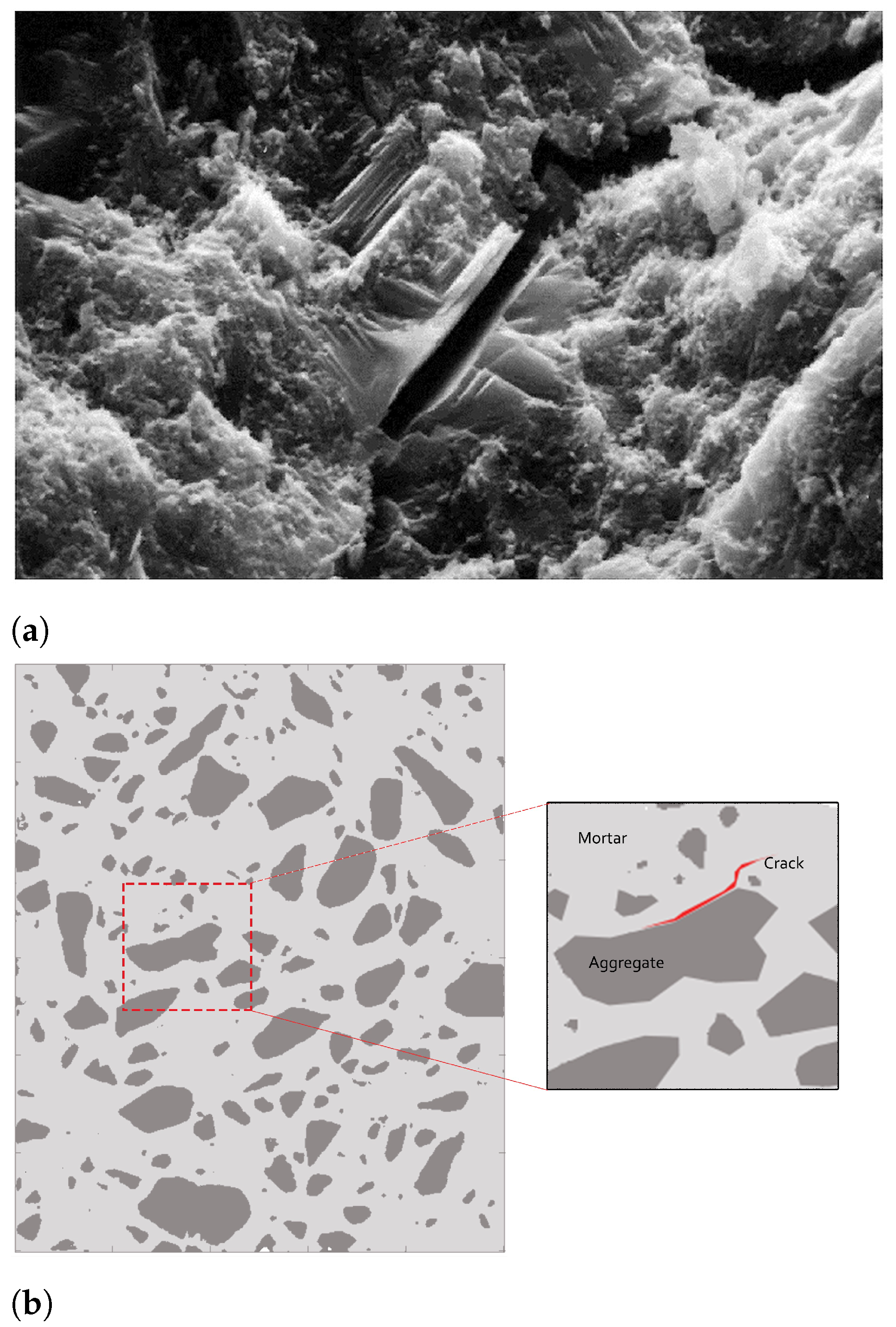
In recent years, many university researchers have studied the problem of concrete damage through the use of Acoustic Emission [1,2,3,4,5]. Acoustic emission (AE) is a natural phenomenon that occurs in the presence of a crack, or a dislocation source, in a material. The response of concrete to the load to which it is subjected in both compression and tension is affected by cracking. Researchers first investigated the microscopic behavior of concrete under compressive stress. The findings in [6,7,8] show that the stress–strain response of concrete is closely associated with the formation of microcracks, that is, cracks that form at coarse-aggregate boundaries (bond cracks) and propagate through the surrounding mortar (mortar cracks), as shown in Figure 1.
During the early studies on microcracking, concrete was considered to be composed of two brittle, linear and elastic materials: the paste and cementitious aggregates; moreover, the main causes of the non-linear stress–strain behavior of concrete in compression were considered to be microcracks [6,8]. This approach changed in the 1970s. Cement is a non-linear softening material, as is the mortar that makes up the concrete. The nonlinear compressive behavior of concrete depends largely on the response of these two materials and depends less than originally thought on the bond and microcracks of the mortar [9,10,11]. However a significant portion of the nonlinear deformation of mortar and cement is due to the formation of microcracks several orders of magnitude smaller. The effect of macroscopic cracks on the performance and failure characteristics of concrete is also an important factor. They reduce the characteristic resistance of the material and are formed as a union of microcracks in a given neighborhood. In the analysis of the AE signals generated in concrete, it is assumed that each fracture consists of the sum of many microcracks that join to compose a larger fracture. The largest crack will be characterized by the maximum amplitude of the AE signal. The signal is recorded by special acoustic emission sensors operating at precise resonance frequencies and in the ranges between 50 and 400 kHz [12,13,14]. These frequencies represent the range in which the signal develops within the concrete under stress.
Different methods for studying and analyzing these signals can be found in the literature. One of the most recent and interesting methods is the one that links the b value to AE signals. This method is based on the Gutenberg Richter law (GBR), typically used in seismology to study earthquakes [15,16]. The GBR law defines the relationship between the magnitude and the total number of recognized earthquake events in a region during a predetermined time interval. The b-value parameter, defined within the framework of the GBR law, is used to select AE signals that identify critical damage events [17,18]. Specifically, critical AE signals are selected provided that the b-value has a value in the neighborhood of 1. In fact, in this neighborhood, the AE signals have the highest amplitude and are generated by the most important damage events. This extension of a law of seismology to AE was possible because of the strong similarities between acoustic waves and seismic waves. In fact, both types of waves can be classified as damped waves, characterized by a peak and a progressive damping of the signal. This technique is used to detect major cracks that develop in concrete during different types of tests, such as the compressive test or the three-point test. To date, the interest of the scientific community has focused on the use of this and other methods to study composite materials and concrete under flexural stresses in order to facilitate the identification of the area where damage develops. The study of a brittle material, such as concrete, is more challenging because the entire section of the compression-proof material is subjected to stress, making the area early damage development uncertain. In addition, we briefly mention that another aspect that could influence the propagation of AE in a porous material, such as concrete, is the aggression of the material by some chemical pollutant [19,20].
Another interesting issue is the localization of the damage which is the source of AE. This is one of the most important criteria for damage detection and classification. In [21], the authors investigated a microseismic/acoustic (MS/AE) emission source localization method to predict and control the formation of potentially dangerous fractures in complex structures. In order to avoid localization errors induced by both the irregular shape of concrete structures and the propagation velocity of elastic waves, a velocity-free MS/AE source localization method was developed. The method avoids repetitive manual training by using equidistant grid points for path finding, introducing the A* search algorithm and using grid points to fit complex structures and velocity-free source localization. Other localization methods not aimed at damage localization in fragile materials such as concrete but useful for improving the accuracy of indoor localization are based on the integration of inertial navigation system (INS) with wireless sensor network (WSN) [22].
Several studies have been carried out by researches in relation to AE source localization and are available in the literature [23,24]. These different methods are characterized by uncertainty about the location of cracks and need to be improved for brittle materials subject to compression. They often depend on the wave propagation velocity in the material, and no index exists in the literature for materials such as concrete, but there are uncertain ranges from 5000 to 10,000 m/s. A possible approach to validating and seeking damage in concrete is based on the use of X-ray tomography. This technology is still in the experimental stage, and it could provide 3D reconstructions of the specimens before and after testing, allowing the exact location of cracks to be obtained, with results comparable to those obtained with localization methods. Concrete is an X-ray shielding material, and so far, the experimentation has only been applied to small specimens [25].
This paper addresses the theoretical foundation of a localization method for crack detection in a concrete sample based on the time of arrival of the elastic wave, generated by the crack formation, to a group of sensors positioned on the boundary of the sample. The following Section 2 is devoted to writing the equation of motion for the elastic wave, with a body force term which accounts for the sudden formation of a crack. A localization method is described on Section 3, and, finally, some numerical experiments are performed in Section 4 to assess the validity of the method.
2. Equations of Motion
We consider a sample of concrete, which is subject to pressure stress along the vertical direction. The sample is not homogeneous, but it is possible to extract effective elastic properties, so that it can be modeled as an elastic material with Lamé constants , . The compression stress will eventually produce one or multiple cracks inside the sample, which will cause the propagation of elastic waves. The waves can be detected by some sensors located on the boundary of the sample. Here, the relevant information is the time of detection of the wave arrival at each sensor. The problem that we want to solve is the identification of the position of the cracks by using only the above information. Together with the position, we also want to determine the time of the cracks’ formation.
Before discussing the identification procedure, we present the mathematical model of the direct problem, that is, the propagation of an elastic wave in a concrete sample, originated by a single pointsize crack formation inside it at a given time. We give a brief summary of the classical theory, following [26]. Let us consider a displacement field , with space coordinates and time . Here, represent the region occupied by the sample. The displacement field satisfies the dynamic elastic equilibrium equations:
where is the density, depending on space; is the stress tensor; and is a body force term, depending on space and time. For an isotropic medium, Hooke’s law provides a linear constitutive relation for the stress tensor in terms of the strain tensor , that is,
where and are Lamé’s first and second parameters, respectively. They can be expressed in terms of the Young modulus E and the bulk modulus K by and .
In component form, let , , and the notation denote the derivative of with respect to t, the notation denote the derivative of with respect to , . Using Einstein’s convention of implicit summation for repeated indices, we have:
where is the Kronecker delta, and Equation (1) becomes:
The body force components will be chosen to model a sudden separation of two sides of a fault localized in a point, which might be thought of as an infinitesimal planar crack with a prescribed normal direction. Following the classical paper by Burridge and Knopoff [27], let us assume that the displacement and its derivatives present a discontinuity across a surface embedded in . Let denote the normal direction to , and , the discontinuity of , across in the direction . Then, the body force equivalent is given by:
where is the Dirac delta function and is its (distributional) derivative with respect to . The occurrence we want to describe is explicitly considered in [27], in the special case when collapses to the origin and . Then, we have , , , where is the Heaviside function, and the equivalent body force has components:
In compact form, introducing the diagonal matrix , we can write:
In the general case, we need to transform to new coordinates with respect to a basis , such that . We then apply the previous result, and finally, we perform the inverse transformation. Introducing the rotation matrix R, with , defined by , , we have:
Here, we have used the inverse transformation and the property . The body force term can be translated to an arbitrary point by replacing with inside the Dirac delta functions.
Summing up, we model the formation of a crack in a concrete sample by Equation (3), with
where the parameter is the normal direction to the crack and comprises three angular variables in three dimensions (Euler angles) or an angular variable in two dimensions, and the parameter is the location of the crack, that is, three coordinates in three dimension, or two coordinates in two dimensions, for a total of six parameters in three dimensions, or three parameters in two dimensions. These parameters are treated as random variables. The equations are supplemented with homogeneous Neumann boundary conditions on the boundary of the space domain and with zero initial data.
Once we have a model for the propagation of the elastic wave generated by the formation of a point crack, we need to address another important element for the definition of the localization problem, described in the following section, that is, the velocity of propagation of the elastic wave. To find the characteristic velocities, we look for a plane wave solution for (3), with zero body force, of the form:
where and are the amplitudes, is the wavenumber vector, and is the angular frequency. Plugging (8) in Equation (3) with , we find the eigenvalue problem:
for the eigenvalue and eigenvector . The solutions are:
corresponding to dilatational and isochore waves, with velocities and , respectively. For all the considerations in the next section, we will use the primary velocity to evaluate the ratio between the distance of a sensor from the source of the crack and the corresponding time of travel.
3. Crack Detection
As discussed in the previous section, the location and orientation of a sudden crack are described by the vectors and . We assume to have N sensors, at the positions , with . The i-th sensor detects the arrival of an elastic wave at time , . We assume for simplicity that a crack only develops at the position at time . As a working hypothesis, we also assume that the orientation of the crack is not relevant for the effectiveness of the localization procedure that we will present. We aim to identify and from the reading of the arrival times , .
We know that the speed of the elastic wave in the direction of the front propagation is , so we have:
To solve for , we need to minimize the residuals
that is, to minimize the function given by their quadratic norm,
This is a nonlinear least squares problem which can be solved by the Gauss–Newton method. Before discussing this method, we present a strategy for choosing a good initial guess by means of the simple intersection algorithm. The starting point is Equation (10), which, after squaring both members, can be written in the form:
Finally, subtracting the first equation from the remaining equations, we can eliminate the nonlinear terms on the right-hand side and obtain an estimated value of :
where the dagger denotes the Moore–Penrose pseudo-inverse of a matrix, that is:
Now, we can go back to the Gauss–Newton method, replacing the original least squares problem for (11) with a sequence of linear least square problems. We write (11) as:
and the minimum occurs when the gradient of S with respect to is zero:
with
Assuming we know an approximation of the solution for , we set:
and we solve for using the following approximate gradient equations:
In compact form, introducing
we can write:
which yields the gradient equations:
4. Numerical Simulations
To validate the localization method developed in the previous sections, we perform a two-dimensional numerical simulation of Equation (3), with a body force given by the expression (7). Then, the sensors will be represented by a set of points on the boundary, and the reading of a specific sensor by the the first time at which the displacement vector at that point becomes different from zero.
We consider the two-dimensional version of system (3) in a rectangular sample , with homogeneous Neumann boundary conditions and zero initial value:
Here, for simplicity, we do not use indices for the dependent and independent variables, so is the displacement vector, depending on space variables and time t, and the body force is . Let be the angle formed by the infinitesimal crack line with the x-axis, so that the tangent vector to is , and the normal vector is , and let be the location of the crack. Then, the rotation matrix R and the diagonal matrix D are given by
and the expression (7) which gives the corresponding body force becomes
For the numerical simulations, we use a representation of the Dirac delta:
so that (24) will be replaced by:
The maximum of both components of this function is , so we divide the above expression by this constant to obtain an approximation of the theoretical body force with reasonable magnitude.
To integrate numerically (23) and (24), we use a box-integration method with two staggered grids. We subdivide the interval in subintervals of equal length , the interval in subintervals of equal length , and introduce the primary grid points:
and the dual grid points:
The boxes for the primary grid are rectangles with length and height , centered on the internal grid points :
while the boxes for the dual grid are rectangles with the same size, not touching the boundary, and centered on the internal grid points :
We integrate the first equation in (23) over the primary boxes and the second equation over the dual boxes , obtaining the equations:
Introducing the notation
we can approximate:
which leads to
In the same fashion, we can approximate:
which leads to
Equation (28) has been derived for , and Equation (29) for , . We can extend them to the other values of i and j by using ghost nodes and enforcing the boundary conditions. We introduce the ghost nodes , , , , and the following mirror conditions with respect to the boundary, which enforce homogeneous Neumann conditions for u and v:
In this way, we obtain Equation (28) for the unknowns , , , coupled with Equation (29) for the unknowns , , .
After a standard finite difference approximation with three points for the second-order time derivative, with time step , we obtain the following scheme:
where the superscript denotes the index of the time . The above scheme provides the update for the unknowns on the grid points at time in terms of the same unknowns at times , . To initialize, we use:
where the time second derivatives at can be evaluated from the right-hand sides of (28) and (29) with , .
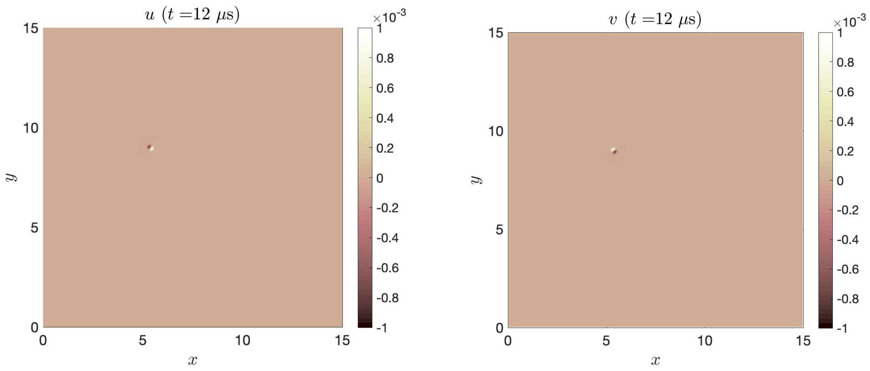
We have solved this system in a square with size 15 cm, with grid points, that is, space step cm and time step µs. We have used Lamé’s parameters GPa, GPa, and density , which are appropriate values for mortar [28]. The numerical scheme has been implemented in Matlab, and the simulation time is approximately ten minutes. A crack formation has been simulated at the position between a couple of adjacent grid points, one on the primary grid and the other one on the dual grid, at a random time µs, with an angle between the crack line and the x-axis. The initial shape of the crack is shown in Figure 2.
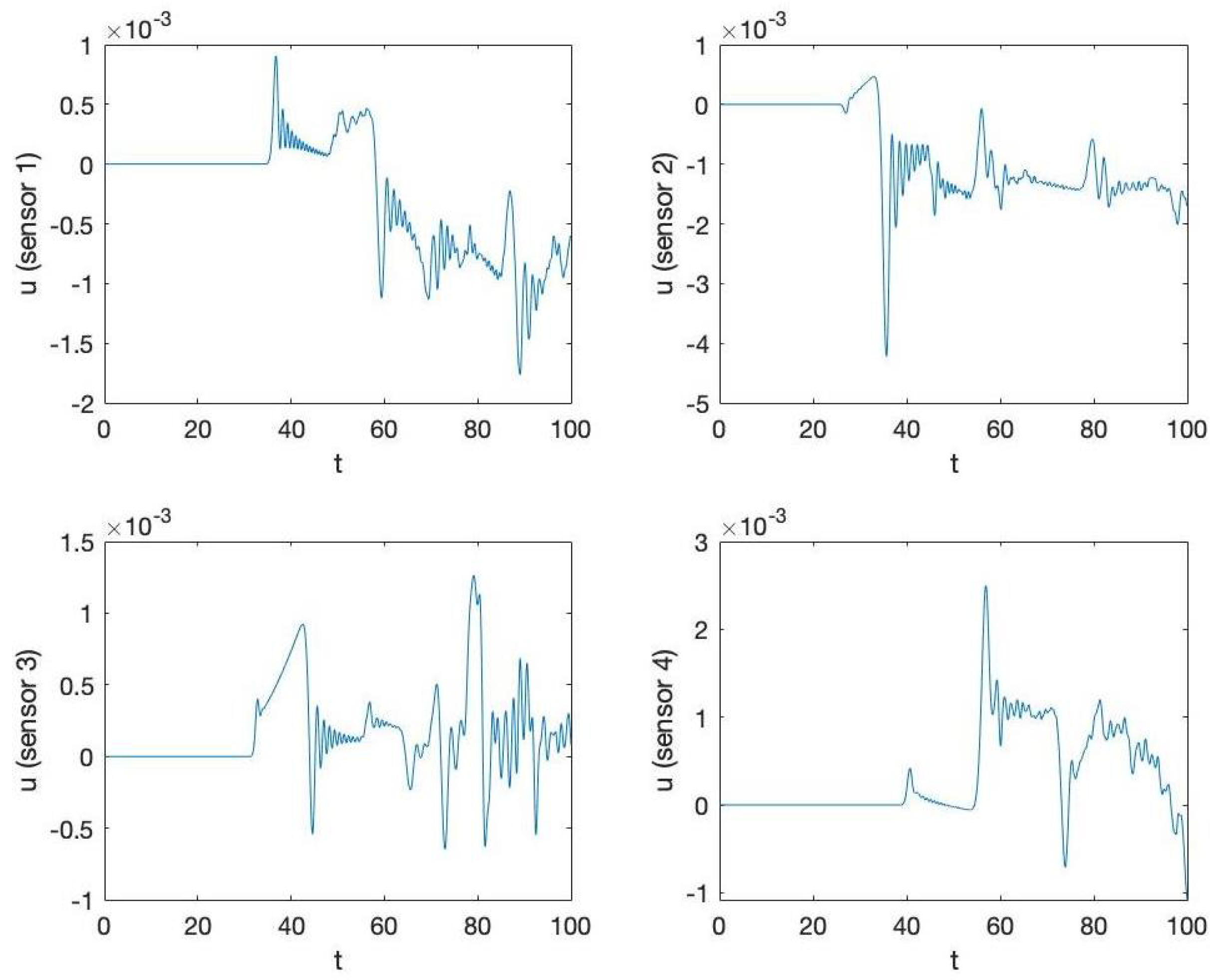
To validate the localization method discussed in Section 3, we have simulated four sensors, located in the positions , , , and . The values of u on each sensor, for all simulation times, are shown in Figure 5. The readings of the sensors should be interpreted as the arrival times of the elastic wave generated by the crack. To discriminate between false readings, we have applied the rule to take the first time for which is greater than 3% of its maximum value on the simulation time. Our preliminary results are quite encouraging. For the simulation performed in this section, the method gives an estimated location of the crack at (5.4438, 8.8606) and an estimated formation time of µs. These values are remarkably close to the real crack location (5.355, 8.955) and formation time , with a relative error of about . It is worth noting that the linear initialization step (14) provides a poor result, estimating the crack at at (negative) time µs, while the nonlinear method reaches convergence with good results after three iteration steps.
5. Conclusions
In this paper, we have revisited the equations of elasticity, including a “body force term to be applied in the absence of a dislocation, which produces radiation identical to that of the dislocation”, citing the classical paper [27] where the general expression of this term was first derived. We have paid special attention to a specific kind of dislocation, “which represents a sudden separation of the two sides of the fault as, for example, an explosion in a plane crack” [27], because this mechanism seems adequate to describe what would happen in a concrete sample under pressure tests which produce microcrack formation. In Equation (7), we provide a generalization of the simple example in [27], which depends on the location of the crack and on its orientation. This is particularly relevant since, to our knowledge, no exact source function of acoustic emissions has been identified as of yet. For 2D numerical simulations, an approximated version of (7) has been provided in (25). The numerical results indicate that indeed it is a reasonable source.
The proposed method, through an experimental setup of acoustic emission acquisition, as shown in [17], could ensure the localization of cracks within concrete structures without the use of destructive or nondestructive survey methods. In fact, the latter are either difficult to implement, as in the case of X-ray microtomography, or are inaccurate, as in the case of ultrasonic methods. The data acquired in [17] can be processed by the method proposed in the article and, based on the acquired delay times, provide the location of the crack associated with the acoustic emissions.
This paper also aimed at establishing a theoretical foundation for the above localization method, based on the arrival times of acoustic emissions produced by a crack’s formation to a group of sensors dislocated on the boundary of a concrete sample. The preliminary results that we have obtained are quite encouraging and suggest the validity of the proposed localization method. Still, we believe that it is possible to improve the accuracy of the method. In our opinion, the main point is to improve the simulation of the reading of the sensors. Here, two observations are in order. The first one is that it is not clear how to determine to correct arrival time, due to the complexity of the detected signals, as shown in Figure 5. We have used the 3% rule, as stated at the end of last section, but other rules might need to be assessed. The second observation is that we made a working assumption that the arrival times do not depend on the angle formed by the crack line with the x-axis. Actually, there is numerical evidence that such dependence does exist. In other words, for deriving an improved localization method, it might be necessary to include the parameter as an additional value to be extracted from the sensors’ readings, together with the time of formation and the position of the crack. This extension of the localization method will be the subject of a subsequent paper.
Author Contributions
Conceptualization, C.S.; Data curation, F.D.; Formal analysis, G.A.; Methodology, F.D. and C.S.; Supervision, G.A.; Writing—original draft, G.A.; Writing—review & editing, F.D. and C.S. All authors have read and agreed to the published version of the manuscript.
Funding
This research received no external funding.
Institutional Review Board Statement
Not applicable.
Informed Consent Statement
Not applicable.
Data Availability Statement
Not applicable.
Acknowledgments
This paper has been performed under the auspices of the G.N.F.M. of INdAM.
Conflicts of Interest
The authors declare no conflict of interest.
References
- Topolář, L.; Kucharczyková, B.; Kocáb, D.; Pazdera, L. The acoustic emission parameters obtained during three-point bending test on thermal-stressed concrete specimens. Procedia Eng. 2017, 190, 111–117. [Google Scholar] [CrossRef]
- Tsangouri, E.; Karaiskos, G.; Deraemaeker, A.; Van Hemelrijck, D.; Aggelis, D. Assessment of acoustic emission localization accuracy on damaged and healed concrete. Constr. Build. Mater. 2016, 129, 163–171. [Google Scholar] [CrossRef] [Green Version]
- Geng, J.; Sun, Q.; Zhang, W.; Lü, C. Effect of high temperature on mechanical and acoustic emission properties of calcareous-aggregate concrete. Appl. Therm. Eng. 2016, 106, 1200–1208. [Google Scholar] [CrossRef]
- Van Steen, C.; Nasser, H.; Verstrynge, E.; Wevers, M. Acoustic emission source characterisation of chloride-induced corrosion damage in reinforced concrete. Struct. Health Monit. 2022, 21, 1266–1286. [Google Scholar] [CrossRef]
- Xu, J.; Niu, X.; Yao, Z. Mechanical properties and acoustic emission data analyses of crumb rubber concrete under biaxial compression stress states. Constr. Build. Mater. 2021, 298, 123778. [Google Scholar] [CrossRef]
- Thomas, T.C. Mathematical analysis of shrinkage stresses in a model of hardened concrete. AIC J. Proc. 1936, 60, 371–390. [Google Scholar]
- Shah, S.P.; Chandra, S. Fracture of concrete subjected to cyclic and sustained loading. AIC J. Proc. 1970, 67, 816–827. [Google Scholar]
- Shah, S.P.; Winter, G. Inelastic behavior and fracture of concrete. AIC J. Proc. 1966, 63, 925–930. [Google Scholar]
- Spooner, D.C.; Dougill, J.W. A quantitative assessment of damage sustained in concrete during compressive loading. Mag. Concr. Res. 1975, 27, 151–160. [Google Scholar] [CrossRef]
- Maher, A.; Darwin, D. Mortar Constituent of Concrete in Compression. ACI J. Proc. 1982, 79, 100–109. [Google Scholar]
- Cook, D.J.; Chindaprasirt, P. Influence of loading history upon the compressive properties of concrete. Mag. Concr. Res. 1980, 32, 89–100. [Google Scholar] [CrossRef]
- Ohtsu, M. Elastic wave methods for NDE in concrete based on generalized theory of acoustic emission. Constr. Build. Mater. 2016, 122, 845–854. [Google Scholar] [CrossRef]
- Scuro, C.; Lamonaca, F.; Porzio, S.; Milani, G.; Olivito, R.S. Internet of Things (IoT) for masonry structural health monitoring (SHM): Overview and examples of innovative systems. Constr. Build. Mater. 2021, 290, 123092. [Google Scholar] [CrossRef]
- Rehman, S.K.U.; Ibrahim, Z.; Memon, S.A.; Jameel, M. Nondestructive test methods for concrete bridges: A review. Constr. Build. Mater. 2016, 107, 58–86. [Google Scholar] [CrossRef] [Green Version]
- Gutenberg, B.; Richter, C.F. Magnitude and energy of earthquakes. Nature 1955, 176, 795. [Google Scholar] [CrossRef] [Green Version]
- Sagar, R.V. A parallel between earthquake sequences and acoustic emissions released during fracture process in reinforced concrete structures under flexural loading. Constr. Build. Mater. 2016, 114, 772–793. [Google Scholar] [CrossRef]
- Carnì, D.L.; Scuro, C.; Lamonaca, F.; Olivito, R.S.; Grimaldi, D. Damage analysis of concrete structures by means of acoustic emissions technique. Compos. Part B Eng. 2017, 115, 79–86. [Google Scholar] [CrossRef]
- Carnì, D.L.; Scuro, C.; Lamonaca, F.; Olivito, R.S.; Grimaldi, D. Damage analysis of concrete structures by means of b-Value Technique. Int. J. Comput. 2017, 16, 82–88. [Google Scholar] [CrossRef]
- Alì, G.; Furuholt, V.; Natalini, R.; Torcicollo, I. A mathematical model of sulphite chemical aggression of limestones with high permeability. Part I. Modeling and qualitative analysis. Transp. Porous Media 2007, 69, 109–122. [Google Scholar] [CrossRef]
- Alì, G.; Furuholt, V.; Natalini, R.; Torcicollo, I. A mathematical model of sulphite chemical aggression of limestones with high permeability. Part II: Numerical approximation. Transp. Porous Media 2007, 69, 175–188. [Google Scholar] [CrossRef]
- Dong, L.; Hu, Q.; Tong, X.; Liu, Y. Velocity-free MS/AE source location method for three-dimensional hole-containing structures. Engineering 2020, 6, 827–834. [Google Scholar] [CrossRef]
- Chen, X.C.; Chu, S.; Li, F.; Chu, G. Hybrid ToA and IMU indoor localization system by various algorithms. J. Cent. South Univ. 2019, 26, 2281–2294. [Google Scholar] [CrossRef]
- Carpinteri, A.; Lacidogna, G.; Niccolini, G. Critical behaviour in concrete structures and damage localization by acoustic emission. In Key Engineering Materials; Trans Tech Publications Ltd.: Bäch, Switzerland, 2006; Volume 312, pp. 305–310. [Google Scholar]
- Manuello, A.; Niccolini, G.; Carpinteri, A. AE monitoring of a concrete arch road tunnel: Damage evolution and localization. Eng. Fract. Mech. 2019, 210, 279–287. [Google Scholar] [CrossRef]
- du Plessis, A.; Boshoff, W.P. A review of X-ray computed tomography of concrete and asphalt construction materials. Constr. Build. Mater. 2019, 199, 637–651. [Google Scholar] [CrossRef]
- Achenbach, J.D. Wave Propagation in Elastic Solids; Elsevier: Amsterdam, The Netherlands, 1973. [Google Scholar]
- Burridge, R.; Knopoff, L. Body force equivalents for seismic dislocations. Bull. Seismol. Soc. Am. 1964, 54, 1875–1888, Reprinted in Seismol. Res. Lett. 2003, 74, 154–162. [Google Scholar] [CrossRef]
- Murray, Y.D. Users Manual for LS-DYNA Concrete Material Model 159. Federal Highway Administration Online Report. Publication Number: FHWA-HRT-05-062; May 2007. Available online: https://rosap.ntl.bts.gov/view/dot/38730 (accessed on 1 June 2022).
Figure 1.
Microphotography of a crack in mortar (a) and its schematic representation (b).

Figure 2.
Components of the displacement vector at time µs of crack formation.

Figure 3.
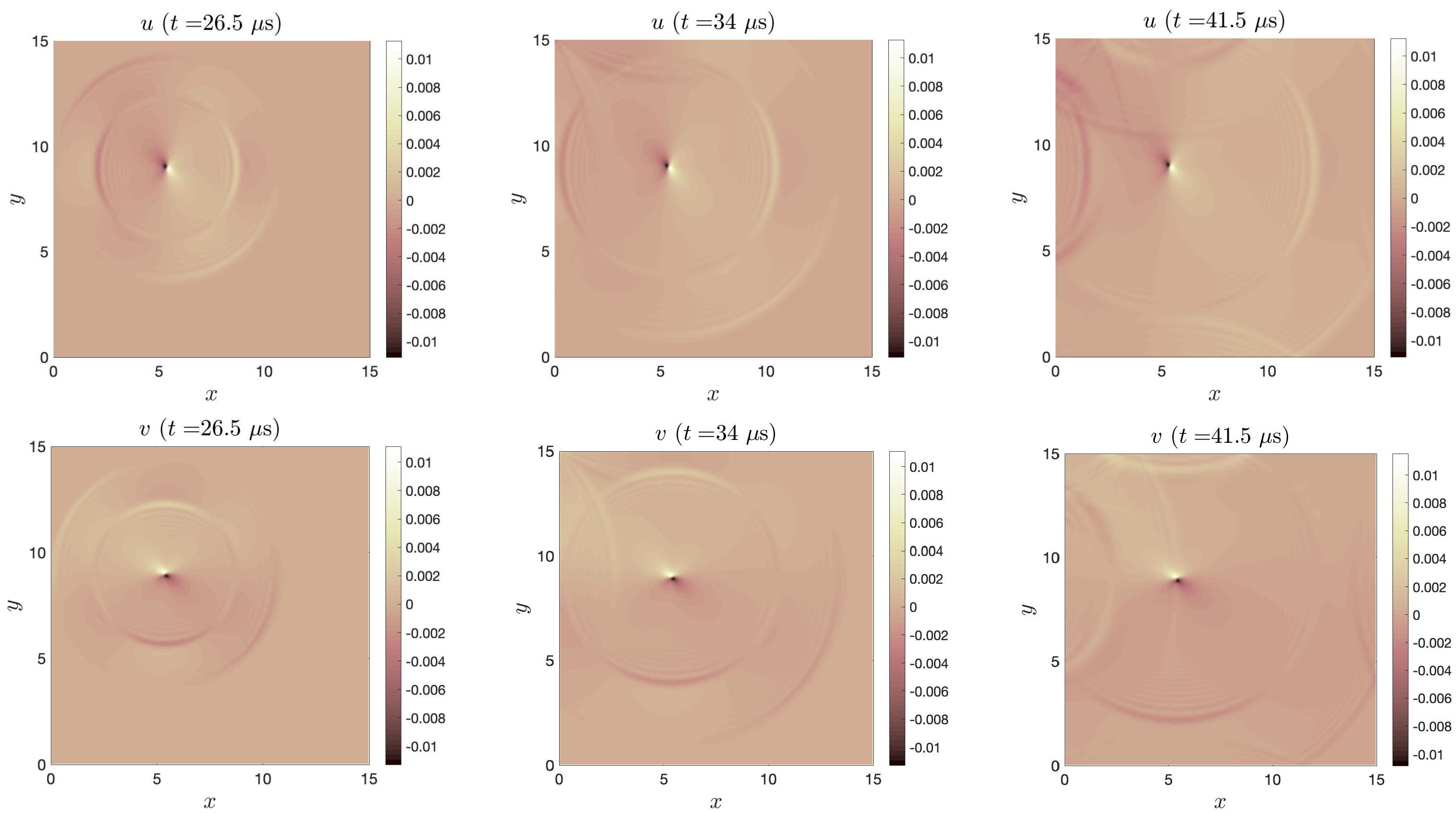
Components of the displacement vector u (top) and v (bottom) at times , 34, and µs.

Figure 4.
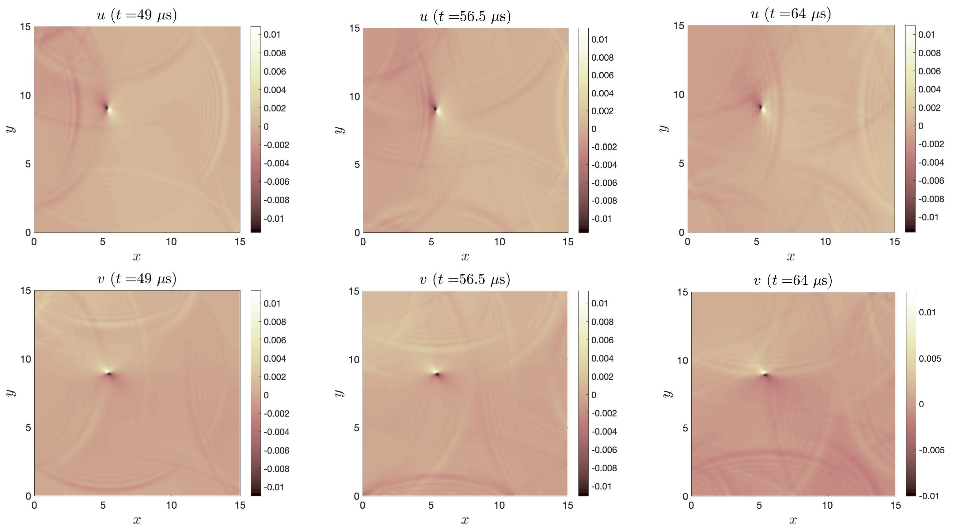
Components of the displacement vector u (top) and v (bottom) at times , and 64 µs.

Figure 5.
Values of the displacement vector u at the sensors’ location, at variance with time.

Publisher’s Note: MDPI stays neutral with regard to jurisdictional claims in published maps and institutional affiliations. |
© 2022 by the authors. Licensee MDPI, Basel, Switzerland. This article is an open access article distributed under the terms and conditions of the Creative Commons Attribution (CC BY) license (https://creativecommons.org/licenses/by/4.0/).
Share and Cite
MDPI and ACS Style
Alì, G.; Demarco, F.; Scuro, C. Propagation of Elastic Waves in Homogeneous Media: 2D Numerical Simulation for a Concrete Specimen. Mathematics 2022, 10, 2673. https://0-doi-org.brum.beds.ac.uk/10.3390/math10152673
AMA Style
Alì G, Demarco F, Scuro C. Propagation of Elastic Waves in Homogeneous Media: 2D Numerical Simulation for a Concrete Specimen. Mathematics. 2022; 10(15):2673. https://0-doi-org.brum.beds.ac.uk/10.3390/math10152673
Chicago/Turabian StyleAlì, Giuseppe, Francesco Demarco, and Carmelo Scuro. 2022. "Propagation of Elastic Waves in Homogeneous Media: 2D Numerical Simulation for a Concrete Specimen" Mathematics 10, no. 15: 2673. https://0-doi-org.brum.beds.ac.uk/10.3390/math10152673
Note that from the first issue of 2016, this journal uses article numbers instead of page numbers. See further details here.