1. Introduction
Climate change is accompanied by dangerous natural phenomena that are becoming more and more frequent. These phenomena inevitably affect human life and daily activities. Research into these issues involves mathematical modeling and analysis of geophysical data, as well as data from numerical and field experiments. The current trend in geodata analysis is associated with the use of machine learning algorithms and artificial neural networks.
Landslides, mudflows, and avalanches are classified as dangerous geological phenomena. These are slope processes associated with the separation of rocks, their movement along the slope under the influence of gravity and leading to irreversible changes in the relief. The study of the descent of landslides, mudflows, and avalanches, as well as their prediction and detection are highly relevant due to the impact of these dangerous phenomena on human life and urban infrastructure. Landslides are distinguished according to the main causes of their occurrence. These are: abrasive, erosional, anthropogenic, and natural/anthropogenic. According to the mechanism of displacement, block landslides, shear, stretching, and liquefaction landslides are classified, respectively [
1].
Data show that between January 2004 and December 2016, landslides killed about 56,000 people in as little as 5000 incidents. The spatial distribution of landslides is uneven, with Asia as the predominant geographic area [
2].
A large number of landslides, avalanches, and mudflows occur in European countries (Switzerland, Austria, Italy, France, and Iceland). Similar dangerous phenomena occur in Russia, for example, in the Krasnodar Territory of the Russian Federation and in the North Caucasus, due to heavy rainfalls in these regions where mountainous terrain is present, and in connection with the development of the territory (linear and areal objects) in recent years [
3]. The amount of precipitation was outstanding in the above territories of Russia (Sochi, Krasnaya Polyana) in 2021. This led to the flooding of mountain rivers and increased the risk of slope flows. Catastrophic descents of mudflows occurred, resulting in damage to road equipment and blockage of roadways [
4].
Mudflows are one of the most complex exogenous geological processes, which integrate the actions of other geological processes. The mudflow is a complex heterogeneous structure consisting of liquid and solid components. The solid fraction consists of mineral particles, which are non-uniform from the granulometric viewpoint.
The most well-known landslide problem involves assessing the stability of a landslide slope for static conditions and seismic impact. Modeling the descent of the slope flow makes it possible to predict the damage caused by this phenomenon and to correctly locate the protective structures and vital objects. Such problems are solved using the finite difference method [
5], the finite volume method [
6], the discrete elements method [
7], the cellular automata method [
8], and hybrid methods. The mudflows can be modeled using a two-fluid model based on the Volume of Fluid model [
9]. The methods listed above are implemented in various commercial and open source software packages MN2D [
10], TITAN2D [
11], and RAMMS.
Previously, the study of avalanches was carried out using computational fluid dynamics methods for Newtonian fluids and analysis of observation data, including the historical data on avalanches in Japan [
12,
13]. Similar work was carried out on avalanches in Switzerland, Austria, and Italy. A series of works on the study of avalanches using laboratory experiment in special trays and measuring equipment for studying avalanches in Iceland were carried out at the University of Iceland [
14,
15]. An experiment with the descent of a snow-water stream in Davos, Switzerland was described in [
16]. Measurements were made for the flow depth for a dry snow avalanche and for a snow-water flow.
Cheng et al. [
17] used Bayesian analysis to calibrate the coefficients of the Spalart–Allmaras turbulence model to correct model deficiencies and reproduce the profile of a turbulent boundary layer over a flat plate. Among similar works, the coefficients were already calibrated in the
turbulence model when studying the process of the propagation of impurities in the process of urban development [
18].
Bayesian analysis is often used to calibrate the RANS closures turbulence models to improve forecast accuracy without losing computational efficiency (as was done for
model with Launder-Sharma damping functions,
Wilcox model, Spalart–Allmaras and Baldwin–Lomax models [
19,
20]). De Zordo-Banliat et al. applied Bayesian analysis to compressor cascades to obtain a set of calibrated turbulence model parameters due to the inadequacy of the original model [
21].
Kotaro Matsui et al. [
22] proposed a new set of calibrated coefficients that improved the ability of the Spalart–Allmaras model to predict compressor cascade flow angular separation. A comprehensive review of turbulence model uncertainties is given in the paper of Xiao and Cinnella [
23].
A comprehensive analysis of climatic, geological, and hydrological data was applied to model and predict the slope flows. In the scope of recent trends, huge streams of data received from satellites, from the experiments, and from mathematical modeling are processed using machine learning, which makes it possible to develop efficient models of these processes [
24,
25].
Recently, several new optimization and machine learning methods have been proposed. In [
26], a new method of regret analysis, called stochastic p-robust optimization, has been proposed, which allows to simultaneously take advantage of stochastic optimization and robust optimization methods to study the optimal operation of a hybrid energy system.
A learning-based method for building driving-signal aware full-body avatars was presented in [
27]. The model was a conditional variational auto-encoder that could be animated with incomplete driving signals, such as human pose and facial keypoints, and produced a high-quality representation of human geometry and view-dependent appearance.
A novel multi-class wind turbine bearing fault diagnosis strategy based on the conditional variational generative adversarial network model combining multi-source signals fusion was proposed in [
28]. The strategy converted multi-source 1D vibration signals into 2D signals, and the multi-source 2D signals were fused by using wavelet transform.
A complementary label adversarial network (CLARINET) was proposed to solve completely complementary unsupervised domain adaptation (CC-UDA) and partly complementary unsupervised domain adaptation (PC-UDA) problems. CLARINET maintains two deep networks simultaneously, with one focusing on classifying the complementary-label source data and the other taking care of the source-to-target distributional adaptation [
29].
A challenging problem called unsupervised open set domain adaptation (UOSDA) was considered in [
30]. The authors proposed a practical theoretical bound for UOSDA, which contained an effective risk estimator to evaluate the risk on data with unknown classes. In addition, a DNN-based UOSDA method under the guidance of the proposed theoretical bound was put forward. The method can accurately estimate the risk of the classifier on data with unknown classes and adequately align the distributions of data with known classes.
Methods based on convolutional neural networks (CNN) are able to extract stable spatial and spectral features [
31]. A combination of satellite image and topographic data can be used to generalize the extracted features in order to identify slope flows in satellite images [
32,
33].
Calibration of the
models [
34,
35,
36] was mainly carried out for air flows around various profiles. For example, calibration was performed for the flow around airfoils at high Reynolds numbers in a wide range of angles of attack [
37] (as it was noted by the authors, the area of applicability of the suggested modification is limited to flows around airfoils). Calibration was also carried out for the flow around small wind turbines [
38,
39] and around a simple flat plate [
40]. No calibration of the turbulence model for fluid flows with a free surface on a slope under the action of gravity was performed. The work uses a multi-phase model to track the interface to calculate the flow. The effect of this multiphase nature should also be taken into account when using the coefficients of the turbulent model. In the present work, for the first time, the coefficients of the turbulent model are calibrated for the flow of a multiphase fluid under the action of gravity on a slope.
The slope flow model, as a rule, includes several parameters, the values of which cannot be specified in advance but can be selected based on the consistency of the numerical results with the experimental data available. Such a problem is a global optimization problem with a black box objective function because the specific type of the objective function is not known, there exists only the algorithm for calculating its values.
The complexity of the phenomena and processes under study is reflected in the complexity of the corresponding mathematical models and numerical methods for their analysis. Currently, the main (and often the only possible) tool for such an analysis is supercomputer modeling of the object behavior. Open source software is used widely for this purpose. OpenFOAM (an open platform for numerical modeling of continuum mechanics problems) is a well-known example of open source software of this kind [
41].
The growing performance of modern supercomputer systems goes in parallel with the complication of mathematical models of the processes considered that makes performing even a single model calculation (a trial) a computation-costly operation. Consequently, the choice of the optimal values of the model parameters in reasonable time cannot be completed by trying all possible variants by the grid method, i.e., by searching on some regular grid in the range of variation of the parameters. The impossibility of performing a large number of search trials requires applying efficient search algorithms, which would provide an acceptable estimate of a problem solution at a relatively small number of trials using available computational resources.
It is worth noting that most existing methods for finding the optimum of time-consuming black-box functions have some drawbacks. Gradient-based algorithms cannot be used in many cases just because the derivatives of an objective function are unknown while the finite-difference approximations of these derivatives are too computationally costly. At the same time, in general, gradient-based methods only allow finding a locally optimal solution to the problem. Classical direct search methods, which do not require the derivatives, e.g., the Nelder–Mead method [
42] or the Hooke–Jeeves method [
43], are also local. As a rule, the application of these methods for solving global optimization problems involves several restarts from random grid nodes, which requires a large number of trials.
Deterministic methods of the Lipschitz global optimization, such as DIRECT [
44], non-uniform coverages method [
45,
46], diagonal [
47], and simplicial [
48] methods guarantee (in the limit) convergence to the global solution of the problem but may require a large number of search trials. Finally, heuristic methods, e.g., differential evolution or simulated annealing, also require a very large amount of computations of the functions to obtain good estimates of the solutions in global optimization problems and at the same time lose in quality to the deterministic algorithms [
49,
50].
So far, the direct application of optimization algorithms to search for the minima of the time-consuming function may appear too computationally costly when a single trial takes a great deal of computation time. A well known method to overcome this problem is to construct an approximation of the objective function (also known as a response surface model or a metamodel or a surrogate model). Computing its values is a computationally inexpensive operation. The approximation is used further to find the minimum. There are many variants of constructing the approximations for multivariate functions. These are various interpolation methods utilizing polynomials, splines, radial basis functions, Kriging, as well as various regression models. Many of these algorithms are used in the development of global optimization methods.
For example, the use of the radial basis functions has been considered in detail in [
51,
52]. In [
53,
54,
55], Kriging-based methods have been proposed. A novel approach to constructing the metamodels and trust-region methods based on these ones has been presented in [
56,
57,
58].
In the present study, we used an efficient global search algorithm [
59,
60] for solving the Lipschitz global optimization problems combined with function approximations based on the regression models. At the first search stage, the algorithm worked with the objective function as a direct method. Then, an approximation of the objective function was constructed using the accumulated information. This approximation was used at the second stage of the search. To construct the approximations, we applied Neural Network Regression (NNR).
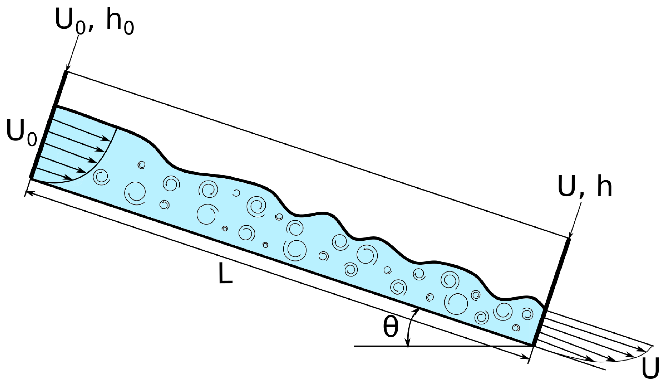
To study the parameters of slope flows, it is advisable to use interdisciplinary approaches from the fields of computational and experimental hydrodynamics, optimization theory, parallel computing, and neural networks. This paper uses the results of an experiment in a chute with a different angle of inclination, a mathematical model for modeling a two-phase flow, global optimization methods, and an artificial neural network. The mathematical model is based on the averaged Reynolds equations and a two-parameter turbulence model.
The turbulence model
contains a number of coefficients calibrated for canonical flows in pipes and channels, air flow around various profiles, etc. [
61,
62,
63]. Calibration of turbulence model coefficients was not carried out for calculating the free surface flows on slopes using the multiphase model for interphase tracking was performed. In this work, the coefficients of the
turbulence model were optimized for calculating the turbulent fluid flow in the chute.
The main part of the paper has the following structure.
Section 2 contains a description of the experiment.
Section 3 describes the mathematical model of turbulent two-phase flows.
Section 4 contains the details of numerical methods.
Section 5 describes the results of numerical experiments.
Section 6 contains a discussion.
Section 7 concludes the paper.
3. Mathematical Model
The Reynolds-averaged Navier–Stokes equations [
65,
66,
67] were used to model the experiment carried out at the Research Institute of Mechanics of Lomonosov Moscow State University. The
turbulence model [
34,
35] was used to obtain the values of the Reynolds stress tensor. The position of the free surface of the flow is determined using the VOF (Volume Of Fluid) method suggested by C.W. Hirt and B.D. Nichols in 1981 [
9]. In this method, the volume fraction of water phase
in the cell is used to determine the free surface so that if
, the cell is considered to be filled with liquid, otherwise—to be filled with air.
The flow in the experimental setup is described by a system of five equations (
1). These are the Reynolds-averaged Navier–Stokes equations (continuity equation and momentum conservation equation). The system also includes a transfer equation for the phase volume fraction to track the interface. The system of equations is closed by two equations of conservation of turbulent kinetic energy and a special dissipation of turbulent kinetic energy, which are used to calculate the Reynolds stresses that arise when averaging the Navier–Stokes equations.
Here,
is the water volume fraction,
is the stress tensor,
is the strain rate tensor,
is the effective viscosity,
is a molecular viscosity,
is a turbulent viscosity,
is the density of the body forces,
is the mixture velocity,
is the mixture density,
is the pressure,
is the specific dissipation rate of the turbulent kinetic energy,
k is the turbulent kinetic energy,
is the blending function (
equals zero away from the wall and the model turns into the
model, while inside the boundary layer
equals one and the
model is realized),
is the strain rate (invariant of
),
,
is the second blending function, and
is the limiter on the growth of turbulence used in stagnation modes. Details can be found in the OpenFOAM package user guide [
68].
The turbulence model contains four coefficients:
,
,
,
.
,
,
are calculated using the weighted average principle:
. By default, the coefficients of the turbulent model are set by the following values [
61,
62,
63]:
The details of the turbulence model description are presented in [
34,
36].
4. Methods
4.1. CFD Numerical Method
To implement the three-dimensional multiphase single-rate approach, the interFoam [
69] solver of OpenFOAM package (v2012, created by Henry Weller in 1989, Bracknell, United Kingdom) was used.
The approximation schemes used in the work are listed below.
The time terms were approximated with first order Euler numerical scheme;
The convection term, the water volume fraction flux term, divergence of the stress tensor term were approximated with second order numerical scheme;
The turbulent kinetic energy flux, the dissipation flux of the specific turbulent kinetic energy term were approximated with first order bounded numerical scheme;
The gradient terms were calculated using Gaussian integration with linear interpolation;
The Laplacian terms were calculated using Gaussian integration with linear interpolation with explicit non-orthogonal correction;
All other terms in the equations were discretized using a central difference numerical scheme.
The second order linear upwind scheme used for the convection term is most efficient and accurate for Reynolds Averaged Navier–Stokes (RANS) simulations [
70].
The PIMPLE algorithm [
71,
72], which was developed to run the equations with a large Courant number, was used to solve the system equations. The PIMPLE is a combination of PISO [
73] and SIMPLE [
74] algorithms.
The conjugate gradient method with preconditioner GAMG is used to solve the system of linear equations for pressure. The GaussSeidel method is used as a smoother. The values for volume fraction of water, velocity, k, are defined using smoothSolver and symGaussSeidel method as a smoother.
4.1.1. Definition of the Calculation Domain
The advantage of mathematical modeling is that the model allows virtual sensors to be placed at any point in the computational domain to measure the values of physical quantities. In the experiment, the physical sensors were placed at the exit from the chute. To compare the results of the experiment and the calculation, the virtual sensors were positioned in the same place.
A section of the experimental chute located between two velocity profile and flow depth measurement points was simulated. The simulations were performed for the thick 10 mm part of the chute where the influence of the side walls was small. The first measured profile was used for the input data for the computational domain. The second one was the object of comparison. The parallelepiped with a size of 590 mm in length, 10 mm in width, and 10 mm in height was used for the numerical domain. We tested the effect of grid resolution. Grid convergence was studied for various grid sizes of
,
,
, and
. For each run, the output velocity profile was compared with the experimental one using the loss function (
5). The values of the loss functions for the last three mesh sizes varied within 0.1%. Therefore, the number of cells was chosen to be
for reasons of reducing computer time while maintaining accuracy.
4.1.2. Initial and Boundary Conditions
The special boundaries for numerical domain were defined: the chute bottom, the chute sides, the upper border for numerical domain, and the inlet and outlet planes.
The following boundary conditions were set:
The solid wall with the no-slip condition was used for the chute bottom;
The zero gradient condition was used for the chute side;
The mixed condition with atmospheric pressure was used for the upper border of numerical domain, no inflow through the border and outflow according to zero gradient condition and fixed value condition for k and ;
The fixed values were used for inlet plane for water volume fraction, velocity profile, k and values;
The zero gradient condition was used for outlet plane.
The mathematical formulation of the listed initial and boundary conditions is presented in the OpenFOAM user manual [
68].
The average value of was 17 which satisfied the model of wall functions. The nutkWallFunction was used for boundary condition for the wall, which provides a wall constraint on the turbulent viscosity, based on the turbulent kinetic energy for both low- and high-Reynolds number turbulence models.
The initial conditions in the problem are set so that the volume is completely filled with stationary air and the liquid flows in through the inlet plane. After a while, the flow is established and measurements are taken on the outlet plane for comparison with the experimental data. The time step is equal to 0.001 s. The flow is considered steady after 5 s.
4.2. Global Optimization Problem Statement
The Globalizer software (Lobachevsky University) was used to solve the optimization problem.
Let us assume that the choice of some set of values of the model parameters is determined by the values of vector
and the quality of the model corresponding to a given value of the vector of parameters is described by the function
. Let us call this function the optimization criterion: a decrease in the criterion value corresponds to a better mathematical model. Additionally, assume that some requirements must be satisfied to guarantee the applicability of the model. Meeting these requirements is usually formulated as the condition for the vector
y to belong to the hyperinterval
D,
So far, the process of choosing the optimal set of the model parameters corresponds to a global optimization problem of the kind:
When optimizing the coefficients of the turbulent model, the Root-Mean-Square Error (RMSE) of differentiation of the calculated flow velocity profile and the experimental one on the outlet plane is taken into account.
is minimized. Here,
is the horizontal component of velocity at the control point obtained by experiment, and
is the horizontal component of velocity at the control point calculated by computational fluid dynamic (CFD),
N is the number of comparison points for the horizontal component of velocity over the flow depth at the outlet plane (right cross-section displayed in
Figure 1). Approximately 10 comparison points are used. Their number is determined by the number of measurements performed in the experiment and varies depending on the change in the flow depth at different chute inclination angles. The points are evenly distributed in depth for the operation of measurement tools used in the experiment.
We will consider the loss function (
5) as the objective function
in the global optimization problem (
4). The problems considered are characterized by the fact that the objective function
is not defined analytically; there is only an algorithm for computing its values at the points of the domain
D. In this case, one search trial corresponds to one computation according to the model and is a time- consuming operation [
75,
76].
Multi-extremal optimization problems have much higher computation costs for solving them as compared to other types of optimization problems since the global optimum is an integral characteristic of the problem being solved and requires investigating the whole search domain. As a result, the search for the global optimum is reduced to constructing some coverage (grid) in some range of parameters and choosing the optimal function value on this grid. The amount of computations may be reduced by constructing a non-uniform coverage of the search domain: the grid should be dense enough in the vicinity of the global optimum and less dense far away from the sought solution.
The assumption that the objective function
satisfies the Lipschitz condition
is a typical and is used in many global optimization methods [
44,
46,
60,
77]. The assumption of this kind is natural enough for many applied problems since the relative variations of the function characterizing the process being simulated cannot usually exceed some threshold imposed by the limited energy of variation. The question of estimating the Lipschitz constant values unknown
a priori arising here can be resolved by introducing some additive schemes [
78,
79].
There are several ways to adapt efficient one-dimensional algorithms for solving multidimensional problems (see, e.g., [
47,
48]). In this study we apply the dimensionality reduction using Peano curve
continuously mapping the unit interval [0, 1] onto the
n-dimensional cube
Algorithms for constructing Peano-type space filling curves and the corresponding theory are considered in detail in [
59,
60].
By using this kind of mapping, the multivariate problem (
4) could be reduced to a univariate problem
An important property of such mapping is that if the function
in the domain
D satisfies the Lipschitz condition, then the function
on the interval
will satisfy a uniform Hölder condition
where the Hölder constant
H is linked to the Lipschitz constant
L by the relation
[
59].
Therefore, we can consider minimization of univariate function
satisfying the Hölder condition.
4.3. The Global Search Algorithm
The algorithm for solving the problem (
4) involves constructing a sequence of points
, where the values of the objective function
are calculated. Let us call the process of calculating the function value (including the construction of an image
) the “trial”, and the pair
, the “trial result”. The set of pairs
makes up the search data collected using the method after carrying out
n steps. The rules that determine the work of the
global search algorithm are as follows.
The first two trials are performed at the boundary points of the segment , i.e., and . The values and of the objective function are calculated, and the counter is set. A next trial point is chosen using the following rules.
Step 1. Renumber points of the set
with subscripts in increasing order of coordinate values, i.e.,
Note that hereinafter superscripts are used to denote the iteration number, and subscripts are used to number the points in order.
Step 2. Supposing that
, calculate values
where the real number
is the method input parameter, and
.
Step 3. For each interval
calculate a characteristic according to the following formula
Step 4. Select the interval
corresponding to the maximum characteristic
Step 5. Execute the new trial at the point
, calculated using the following formula
The algorithm stops when
, where
is the preset accuracy. For estimation of the global optimum, values
are chosen.
A rigorous proof of this algorithm’s convergence is provided in [
59].
4.4. Construction of the Objective Function Approximation
4.4.1. The Use of Neural Networks
There are no universal rules for the choice of the neural network topology to solve a particular problem. However, in [
80] the Kolmogorov theorem has been generalized and it was proved that any continuous function of
N variables can be approximated by a three-layered artificial feedforward neural network with one hidden layer and an error backpropagation algorithm as a learning one with any degree of precision. This theorem is called the Universal Approximation Theorem or the Cybenko theorem [
81].
Neural networks as approximators were implemented in many machine learning libraries. In the present study, MLPRegressor class from scikit-learn machine learning library was used to construct the objective function approximation. It implements a multi-layer perceptron (MLP), which is learned using error backpropagation without activation function in the output layer [
82]. MLPs have demonstrated an ability to find approximate solutions for very complex problems.
A MLP with one hidden layer with a scalar output is shown in
Figure 2.
The left layer called the input layer consists of a set of neurons
representing the input signals (the values of variables). Each neuron in the hidden layer transforms the values from the previous layer with weighted linear summing
where
are the weights of the neurons and
is a special weight, which does not include a factor in the form of an input value. Next, the value obtained is transformed into an output (predicted) value of the layer with a transmission function (the
activation function). The output layer receives the values from the last hidden layer and transforms them into the output values. The network was trained by the error backpropagation method.
We used a three-layered neural network for solving the approximation problem due to the following reasons. From the theoretical point of view, such a network will be sufficient to approximate the function with a high accuracy. From the practical point of view, the use of deep neural networks here will be redundant, because the set of trial results used to build the approximation is small and will not be sufficient to train a deep network.
4.4.2. Selection of the Model Parameters
The choice of the solver, the activation function, the value of the regularization parameter, the number of neurons in the hidden layer, etc., are the variable adjustment parameters of the neural network. For example, for small sets of the multidimensional data, the “lbfgs” solver was demonstrated to be better and faster. This solver is a modification of the Broyden–Fletcher–Goldfarb–Shanno algorithm [
83] and belongs to the quasi-Newton methods. All numerical experiments were carried out using this algorithm. The sigmoidal functions (logistic or hyperbolic tangent) were used as the neuron activation functions. The number of neurons in each layer and the regularization parameter (alpha) were adjusted in the experiments and depended on a particular problem.
In the experiments conducted, we chose the following network architecture:
model = MLPRegressor(activation=’logistic’,
solver=’lbfgs’,
alpha=0.001,
hidden_layer_sizes=(20,),
max_iter=5000,
tol=10e-6,
random_state=10)
4.5. The Use of Approximations in Solving the Optimization Problem
In the present study, we applied the following method of using the objective function approximation in the optimization problems: to construct the objective function approximation using the accumulated search information, to find the minimum of the approximation, and to repeat this process, either until the computation resources are exhausted or until the convergence is achieved.
The method proposed will make sense either in the case when the amount of the search information accumulated is large enough (that allows constructing a relatively precise approximation of a multi-extremal function) or in the case when the problem is similar to a local extremum search problem. The first case corresponds to the final stage of search and can be interpreted as a method of refining the current solution. However, if the objective function is time-consuming, it is impossible to conduct a large enough number of trials. This is where we will encounter an exhaustion of computing resources.
The second case implies constructing a good approximation based on a relatively small number of trials and, in fact, includes an assumption on a weak multi-extremality of the objective function that matches well with the problem considered within the framework of the present study.
The global search algorithm using the objective function approximation can be formulated as follows. Let us assume that the available resources allow for trials to be performed.
At the first stage,
trials are performed using the core global search algorithm from
Section 4.3. In the course of performing the first stage, a set of the trial results
necessary to construct the objective function approximation is accumulated.
At the second stage, the algorithm works using the approximation. To compute the point of the next th trial, the following operations are performed.
Step 1. Using the set of the trial results formed in the course of the algorithm execution, to construct an approximation of the objective function ;
Step 2. Using the core global search algorithm from
Section 4.3 to find the global minimum of the function
and to use this value as the next trial point, i.e.,
;
Step 3. If either the condition or the condition is satisfied, to stop the algorithm. Else, to perform the trial at the point , to store its result in the set , to increment the trial counter , and to proceed to Step 1.
The algorithm proposed here ensures the convergence to the global solution in the case if trials executed at the first stage are sufficient to construct an approximation of the objective function reflecting the main features of its behavior adequately.
5. Results
The simulations were conducted using the supercomputer of Lobachevsky University of Nizhni Novgorod (operated under the Linux CentOS 7.2 operation system). Each supercomputer node included two Intel Sandy Bridge E5-2660 2.2 GHz processors, 64 Gb RAM. The central processor unit had 8 cores. The global optimization methods considered in the present work were implemented in C++ using GCC 5.5.0 compiler and Open MPI v4.1.1. To construct the objective function approximations using a neural network, scikit-learn machine learning library from Python 3.9 was applied. To numerically solve the problem described in
Section 3, the open source CFD software OpenFOAM v2012 [
84] was used.
Before starting the calibration, a small study of the significance of each of the 12 coefficients of the turbulent model was carried out. As a result, it was revealed that the coefficients , , , and make the most significant contribution to the calculation results. It was decided to calibrate these coefficients. These coefficients determine the dissipation rate of turbulent kinetic energy, the Reynolds stress, the diffusion fluxes of turbulent kinetic energy, and the specific dissipation rate. The coefficient is used in the mixing functions that describe the mechanism for switching between the and models. The coefficient determines the turbulent viscosity. characterize the diffusion flux of the kinetic energy of turbulence. characterize the diffusion flow by the specific rate of dissipation of the kinetic energy of turbulence.
The initial values of the coefficients are
One calculation of the objective function for given values of parameters took 15 min in average with the use of 8 MPI-processes per node.
The optimal values of parameters were adjusted for pairs, the values of the remaining parameters were fixed. First, a pair of the most important parameters and was selected. To investigate the optimization problem posed, both possible approaches to solving it were applied: without the use of the objective function approximation and with the use of the approximation.
In the first experiment, the global search algorithm described in
Section 4.3 was applied without the use of approximation. The parameters of the method were set as follows:
and
. In 24 h, 100 iterations of the algorithm were performed; the required accuracy was not achieved.
In the second experiment, the approach described in
Section 4.5 was applied to solve the same problem. First,
iterations of global search algorithm were performed. Afterwards, the algorithm employing the approximation with the neural network was started. A total of
iterations of the algorithm were performed, after that the algorithm stopped on accuracy. As a result, the best value of the objective function 0.375 was found. The total search time was reduced to 16 h, which ensured a more accurate solution for the problem in a reasonable amount of time.
The trial points and the approximating function plotted according to these points using the neural network are presented in
Figure 3 (the parameters
and
were varied). Several local minima are clearly visible. Our analysis showed good agreement between the regression model and experimental data. The
score and the RMSE between the model predictions and the simulated results are equal to 0.976 and 0.098, respectively.
The best values of parameters and found were fixed, and then optimization in parameters , and was performed. However, no significant improvement of the objective function by optimizing on these parameters was achieved: the value of 0.365 was obtained.
As a final result, the following values of the coefficients of the model were obtained:
Figure 4 shows the resulting velocity profiles
as a function of flow depth
h on the exit plane for various slope angles.
During the process of calibration, the minimization of the loss function (
5) was achieved, as shown in
Table 2.
Figure 4 and
Table 2 show a decrease in the discrepancy between the calculated velocity profile and the experimental one for two out of three experiments. Optimization for the three experiments combined (their loss functions were summarized) was used in order to avoid the model overfitting. In one experiment, an almost perfect coincidence of the calculated velocity profile with the experimental one was achieved, which was not reproduced in other experiments. It should also be noted that the divergence of the velocity profile in the region near the chute bottom is due to the measurement error in the experiment, since it is difficult to measure the velocity with the Pitot tube used in this experiment in the immediate vicinity of the bottom.
The minimum value for the objective function was obtained in the case of the slope angle of 33 degrees. One calculation of the objective function for the given parameters took 15 min in average using 8 MPI processes on a node of the Lobachevsky University supercomputer. Total computation time was 24 h.
6. Discussion
When working on the optimization of the turbulent model coefficients, we faced a number of tasks: creating an interface for automatic interaction between the Globalizer software and the OpenFOAM package; in the process of optimization, we encountered the overfitting problem; and the study of the best loss function was carried out, etc.
Creating an interaction interface between Globalizer and OpenFOAM required the use of the pyFoam library to prepare calculation runs. Using the script of this library pyFoamPrepareCase.py, new values of the turbulent model coefficients proposed by the Globalizer software were written into the calculation cases. Next, the calculation was carried out in parallel mode and the result was evaluated using a python script that compared the obtained velocity profile with the experimental one.
A study of various loss functions has been carried out. The loss functions that estimate the absolute error of the velocity profile and the relative error were compared. The relative loss function actually penalizes the area near the bottom more, however, optimization using this loss function did not show significant improvements in the result. This behavior of the calculation is not due to the shortcomings of the numerical model, but rather due to the impossibility of taking velocity values correctly in the region very close to the bottom of the chute. It should be noted that measurements at the point closest to the bottom can have a significant error, due to the measurement method used (the Pitot tube). However, most of the profile was measured quite accurately, since for each measurement point in this stationary experiment, time averaging of 10 s was used. As a result of this study, it was decided to use the absolute loss function, since it showed the best optimization result.
We performed three experiments to avoid overfitting. It was noticed that when optimizing for one velocity profile, the algorithm perfectly calibrated the model, but for other experiments, the result was much worse. When optimizing for three experiments at once, this effect was avoided. The use of the obtained values of the coefficients for fluid flows that are close in dimensionless characteristics will allow a more accurate calculation to be made. However, when generalized to such canonical flows as air flow around different profiles, the use of the obtained values of the turbulent model coefficients is unlikely to show the best result.
This study is part of a larger research effort related to the modeling of currents on the slopes of mountains. These flows are very difficult to study, since they are turbulent multi-phase flows of a non-Newtonian fluid on slopes of complex geometry. For such flows, the use of turbulent models using standard values of coefficients does not predict the flow in the best way. It is necessary to calibrate the turbulence model coefficients or create new turbulence models. We are considering both options. Moreover, a new turbulent model is being developed based on the neural network. However, the use of neural networks requires hybrid computing clusters, which is not always possible. As a result, it is important to be able to obtain a solution of sufficient accuracy using the classical turbulent model. This problem requires the calibration of the coefficients, which was done in this work for the Newtonian medium. Optimization algorithms were developed and tested, which can later be used to calibrate the coefficients of any turbulent models. The next stage of the study is to set up an experiment with a non-Newtonian fluid and calibrate the coefficients of the turbulent model according to the developed algorithm.
We also note that when searching for the optimal model parameters, optimization was carried out first with respect to the parameters and , then optimization in , and was performed. This approach makes it possible to find a good solution in a reasonable amount of time. The search for a global optimum for all parameters at once would require orders of magnitude more trials and time. This effect is a key difference between global optimization and local optimization problems, in which the costs do not grow as fast.
In terms of solving a time-consuming optimization problem with a black-box objective function, it is interesting to compare the method used for solving the problem, which uses objective function approximation by a neural network, with the methods that use kriging-based approximations. Methods of this class work well in problems with a small number of local extrema. However, in essentially multi-extremal problems the computational costs (number of objective function evaluations required for solving the problem) increase significantly.
7. Conclusions
In this work, a two-phase flow in a chute was simulated using the interFoam solver, the URANS mathematical model, and the turbulence model. In the optimization process, six coefficients were investigated in pairs, which make the greatest contribution to the value of turbulent viscosity.
The results of calculating the velocity profiles were compared with experimental data obtained at the Research Institute of Mechanics, Moscow State University, at different sections depending on the angle of inclination of the chute. The search for the optimal coefficients of the turbulence model was performed by minimizing the objective function of the divergence of the velocity profile in the chute.
The search for the global minimum of the objective function was performed using the global search algorithm implemented in the Globalizer software [
85]. In addition, a fully connected neural network with one hidden layer was used to approximate the values of the objective function by the values of the coefficients in the turbulence model. The MLPRegressor class from the scikit-learn library was used to build the objective function approximation.
Based on the results of the study, the following conclusions were drawn.
It is good practice to calibrate the turbulence model coefficients if necessary to improve the accuracy of the calculations. As shown in the present study, it is possible to improve the accuracy by up to 10%.
To perform optimization, at least two, or preferably three datasets should be used. Otherwise, an overfitted model may result. Using a neural network to predict the CFD calculation significantly reduced the optimization time while maintaining the quality of the resulting solution.
The developed calibration algorithm is reliable and can be applied to other models. The algorithm has such advantages as a parallel mode, it can be used to search not only for local, but also for global minima, and can optimize several parameters at once. According to the results of the study, the Globalizer software has performed quite well and will be used in further work.
The OpenFOAM software also shows good results due to code modularity and good documentation. These advantages have made it easier to write a software module for the interaction between the optimizer and OpenFOAM. OpenFOAM also has a high degree of parallelization and can be used to solve a fairly wide range of tasks.
In the present work, an interdisciplinary approach was utilized, which helped us to find the optimal values of six turbulence model parameters using the OpenFOAM open platform and the Globalizer. In the future, it is planned to continue improving the turbulent models, including the development of a turbulent model based on a neural network. The Globalizer software will be used to optimize the model parameters.


 ,
, 


