
Discriminative Convolutional Sparse Coding of ECG Signals for Automated Recognition of Cardiac Arrhythmias


Nanchang Key Laboratory of Medical and Technology Research, School of Advanced Manufacturing, Nanchang University, Nanchang 330031, China
*
Author to whom correspondence should be addressed.
Mathematics 2022, 10(16), 2874; https://0-doi-org.brum.beds.ac.uk/10.3390/math10162874
Submission received: 13 July 2022
/
Revised: 8 August 2022
/
Accepted: 9 August 2022
/
Published: 11 August 2022
(This article belongs to the Special Issue Advances in Artificial Intelligence and Statistical Techniques with Applications to Health and Education)
Abstract
:Electrocardiogram (ECG) is a common and powerful tool for studying heart function and diagnosing several abnormal arrhythmias. In this paper, we present a novel classification model that combines the discriminative convolutional sparse coding (DCSC) framework with the linear support vector machine (LSVM) classification strategy. In the training phase, most existing convolutional sparse coding frameworks are unsupervised in the sense that label information is ignored in the convolutional filter training stage. In this work, we explicitly incorporate a label consistency constraint called “discriminative sparse-code error” into the objective function to learn discriminative dictionary filters for sparse coding. The learned dictionary filters encourage signals from the same class to have similar sparse codes, and signals from different classes to have dissimilar sparse codes. To reduce the computational complexity, we propose to perform a max-pooling operation on the sparse coefficients. Using LSVM as a classifier, we examine the performance of the proposed classification system on the MIT-BIH arrhythmia database in accordance with the AAMI EC57 standard. The experimental results show that the proposed DCSC + LSVM algorithm can obtain 99.32% classification accuracy for cardiac arrhythmia recognition.
Keywords:
electrocardiogram signal; discriminative convolutional sparse coding; dictionary filter learning; linear SVMMSC:
68U011. Introduction
Electrocardiogram (ECG) is used to record cardiac activity and detect different abnormalities in cardiac function and is a commonly used non-invasive tool for non-invasive diagnosis of cardiac arrhythmias. However, visual analysis is extremely limited and imprecise due to the large amount of information contained in the ECG, which may lead to misdiagnosis or inaccurate detection of arrhythmias. Therefore, computer-aided analysis helps doctors to detect cardiac arrhythmias quickly and efficiently.
The automatic arrhythmia detection system mainly includes feature extraction, feature selection, and classifier construction. ECG signal feature extraction techniques can be divided into time-based methods [1,2,3], frequency methods [4,5,6], and time-frequency techniques [7,8]. The time domain features mainly include heartbeat interval, duration parameters, and amplitude parameters. Due to the subtle changes in ECG amplitude and duration, time-based methods do not provide good discrimination [9,10]. Therefore, frequency methods using such as Fourier transform and power spectral density (PSD) and time-frequency methods using wavelet transform are proposed. However, the frequency method does not provide time information from the ECG signal. Time-frequency technology based on wavelet transform is widely used in time-frequency feature extraction of ECG signals. Before the time-frequency feature vectors extracted by wavelet transform are applied to the classifier, it is important to choose the best dimensionality reduction method. Dimensionality reduction methods for linear and non-linear transforms based on wavelet transforms have been proposed [7,11,12,13]. Martis et al. [7] transformed the ECG heartbeat using DWT and then applied independent component analysis (ICA) methods to extract features. The experimental results show that the features extracted using the ICA method combined with a probabilistic neural network (PNN) have better classification results. In the classification step, the most commonly used techniques in ECG signal classification are support vector machines (SVM) [1,14] and artificial neural networks [15].
In this paper, unlike most existing methods, we propose a novel classification model that combines the discriminative convolutional sparse coding framework with the linear support vector machines (LSVM) classification strategy.
The convolutional sparse coding (CSC) model assumes that the signal can be represented as a superposition of a few local filters, convolved with sparse feature maps. The CSC model handles the signal globally, and yet pursuit and dictionary learning are feasible due to the specific structure of the dictionary involved. CSC has been utilized for a variety of computer vision and pattern recognition tasks, such as inpainting [16], image separation [17], image fusion [18], object recognition [19], pedestrian detection [20], and tissue classification [21].
Although the CSC model has achieved state-of-the-art performance in many fields, most of the existing CSC frameworks are unsupervised and ignore label information in the convolutional filter training stage. Chen et al. [22] proposed a novel convolutional sparse coding classification (CSCC) approach, which introduces label information during the training process. The results show that dictionaries trained by convolution with label information can obtain more representative image information and achieve better classification performance. However, in the CSCC model, a set of dictionary filters are trained for each class of data, and then the dictionary filters from all classes build the final discriminative filter bank. This is not an efficient approach. At the same time, the intra-class and inter-class information are not considered, so the coding coefficients have small within-class scatter but large between-class scatter.
How to improve the classification performance of convolutional sparse coding has become a research direction in this field. One of the solutions is to obtain a discriminative dictionary filter bank through training so that the samples of different classes encoded by the dictionary filter bank are discriminative. Methods for learning a discriminative dictionary for sparse coding from training data have been recently proposed. Zhang and Li [23] proposed a discriminative KSVD dictionary learning algorithm. The algorithm incorporated the “classification error” term into the objective function, obtained the dictionary through the KSVD algorithm, and finally realized the classification task through a linear classifier. Yang et al. [24] learned a structured dictionary with class labels by adding Fisher’s discriminant criterion during encoding. The method considers the intra-class and inter-class information in the coding process so that the coding coefficients have small within-class scatter but large between-class scatter. Following the work in [23], Jiang et al. [25] proposed to incorporate a “discriminative sparse code error” term into the objective function to enhance the discriminative power. It forces the signals from the same class to have very similar sparse representations, which results in good classification performance even using a simple linear classifier.
Obtaining a discriminative dictionary for classification by sparse coding has been successfully applied and achieved excellent performance. However, the discriminative dictionary obtained by sparse coding also has shortcomings, that is, it cannot capture the shifted local features in the sample, and at the same time, for high-dimensional signals, there is a curse of dimensionality. The dictionary filter bank obtained by convolutional sparse coding has shift invariance, local features at the sample translation position are extracted by convolution, and there is no curse of dimensionality.
However, how to learn discriminative convolutional dictionary filters with convolutional sparse representation and classification functions by supervised training is still an issue worth investigating. In this work, we propose a discriminative convolutional sparse coding (DCSC) model to learn discriminative dictionary filters for sparse coding of ECG signals. Different from the CSCC algorithm, we explicitly incorporate a label consistency constraint called “discriminative sparse-code error” into the objective function, transform the DCSC model to the Fourier domain to reduce the computational cost [26], and optimize the DCSC model using the alternating direction method of the multiplier framework [27] (ADMM) algorithm. By adding label information to the training phase of the convolutional dictionary filters, the learned dictionary filters encourage signals from the same class to have similar sparse codes, and signals from different classes to have dissimilar sparse codes. To reduce the computational complexity, we use the max-pooling operation on the sparse coefficients. These pooled coefficients are then used as features and fed to an LSVM classifier for the ECG classification task.
Our contributions are as follows:
- We propose a discriminative convolutional sparse coding (DCSC) model in which the “discriminative sparse-code error” is inserted into the objective function.
- In the process of solving the objective function, the DCSC model is first transformed into the Fourier domain, the convolution operation is converted into a multiplication operation, and then the function solution is obtained using the alternating direction method of the multiplier framework.
- The discriminative sparse coefficients are obtained via convolutional sparse coding, then dimensionally reduced by the max-pooling method, and finally fed into the LSVM classifier to complete the ECG classification task.
2. Literature Survey
2.1. Convolutional Sparse Coding
The convolutional sparse coding (CSC) model assumes that a signal can be represented by the sum of M convolutions. These are built by feature maps , each of length N, convolved with M small support filters of length , ∗ denotes convolution, and the CSC model can be formulated as:
where is a regularization parameter. Given the filters, the above problem becomes the CSC pursuit task of finding the representations .
2.2. Convolutional Dictionary Learning
A common approach for convolutional dictionary learning (CDL) [26] entails using a batch of K training data to optimize the filters and sparse coefficient maps. This problem can be formulated as follows:
where the constraint on the norms of dictionary filters is required to avoid the scaling ambiguity between filters and coefficients. We denote the number of filters and the amount of training data by M and K, respectively.
2.3. Label Consistent KSVD
Jiang et al. [25] proposed a label consistent KSVD (LC-KSVD1) algorithm to learn a discriminative dictionary. The objective function is defined as follows:
where denotes the reconstruction error and is the learned dictionary. represents the discriminative sparse-code error, are the “discriminative” sparse codes of input signals used for classification, and is a linear transformation matrix. is the scalar that controls the relative contribution of the corresponding term. are the sparse codes of input signals and is the column vector of . T is a sparsity constraint factor (each signal has fewer than T non-zero items in its decomposition). By adding a discriminative sparse-code error constraint, the LC-KSVD1 model has good classification performance even with a simple linear classifier.
3. The Proposed ECG Signal Classification System
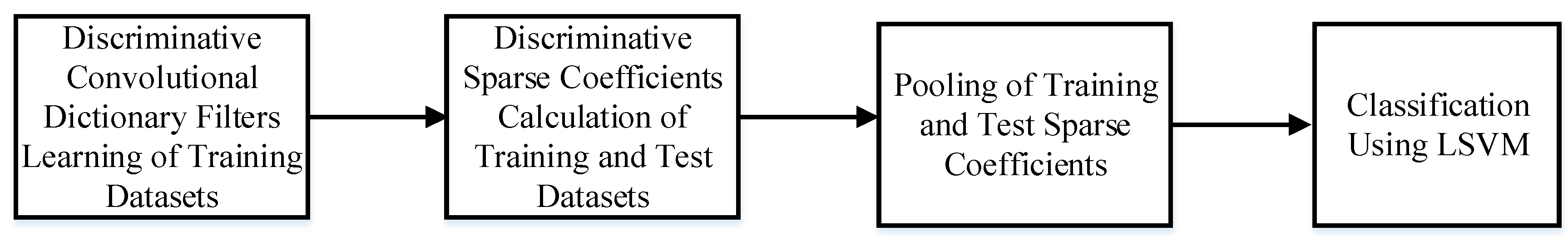
The proposed DCSC-based automatic arrhythmia identification system framework is shown in Figure 1. The proposed method consists of four stages, namely (1) in the discriminative convolutional sparse dictionary filters learning stage, we trained the DCSC model to obtain a discriminative dictionary filter. (2) In the sparse coding stage, we used the CSC model to obtain the discriminative sparse coefficients of the training and the test signals. (3) Pooling was performed on those sparse coefficients to reduce the large amount of data to an appropriate level. More importantly, it is used to obtain a compact representation of features that are invariant to local transformations. (4) In the ECG heartbeat testing stage, we used the pooled coefficients as features and fed them to an LSVM classifier for ECG classification.
3.1. Discriminative Convolutional Sparse Dictionary Learning Model
To improve the discriminative properties of the convolutional sparse coefficients, we incorporate the discriminative terms into the objective function during training. It can be formulated as the following optimization problem:
where is the training data set, . is a regularization parameter and is the scalar that controls the relative contribution of the corresponding terms. and are a set of M dictionary filters, and is a set of coefficient maps corresponding to the dictionary filter and the training data, each having the same size as . is a “discriminative” sparse code corresponding to an input signal , and is the column vector of , whose size is the same as . For example, assuming that , where , are from class 1, , are from class 2, and the length of the training data set N = 6, then can be defined as:
The codes and the dictionary filters and can then be efficiently updated in an alternating manner, as follows.
- Convolutional sparse coding (CSC) step
Given the dictionary filters and , the codes can be updated by using ADMM in the frequency domain.
If we define the linear operators and such that , , and denote
then we can rewrite Equation (6) as
The ADMM algorithm and shrinkage/soft thresholding algorithm can be employed to solve Equation (8), as described in Appendix A.
- B.
- Convolutional dictionary update (CDU) step
In developing the dictionary filter update, it is convenient to switch the index of the coefficient map from to . With the codes fixed, the dictionary filters and can be updated by solving the following optimization problems,
Updating
With the and fixed, the dictionary filters can be updated by solving the following optimization problem,
Addressing the CDL optimization problem (10) over is equivalent to solving the following optimization problem
where is an indicator function [26]. Problem (11) can be solved efficiently using the consensus ADMM method, please refer to Appendix B.
Updating
With the and fixed, the dictionary filters can be updated by solving the following optimization problem,
Addressing the CDL optimization problem (12) over is similar to problem (10), please refer to Appendix B.
| Algorithm 1: The DCSC Algorithm. |
| Input: sample , parameters , Output: Precompute: →, →, Initialize: = = = = 0, while j = 0 to convergence do (CSC step) Compute FFTs of →, →, →, → Compute with the algorithm in Appendix A. Compute inverse FFTs of → (CDU step) Compute FFTs of →, →, → Compute with the algorithm in Appendix B. Compute inverse FFTs of → Compute with the algorithm in Appendix B. Compute end |
We trained the DCSC algorithm with the training data and obtained the dictionary filters. The dictionary filters were then used to obtain the sparse coefficients of both the training and test signals for each class in the sparse coding stage.
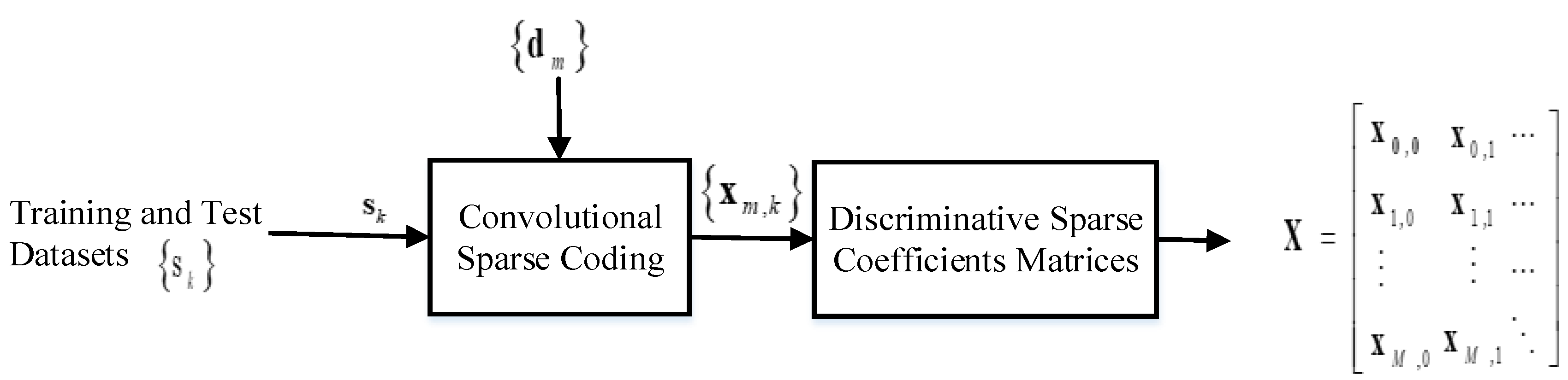
3.2. Sparse Coding of Training and Test Signals
We obtained by employing the DCSC algorithm (Algorithm 1). Sparse coefficient vectors for each signal were obtained by using the CSC algorithm as follows:
The sparse coefficient vectors of each signal thus obtained were then combined column-wise to form a vector of larger dimensions. This process is depicted in Figure 2. The sparse coefficients of these training data were used to train the LSVM model for ECG classification.
3.3. Pooling of Coefficient Matrix
Inspired by the feature extraction methods [29,30], we apply max-pooling methods to each column of the sparse coefficient matrix X.
The max-pooling function
applies a window function to each column of the sparse coefficient matrix X and computes the maximum value in the neighborhood.
These pooled features can then be normalized by
These pooled sparse coefficients from each sub-region are concatenated and normalized to the final feature representation for the classification.
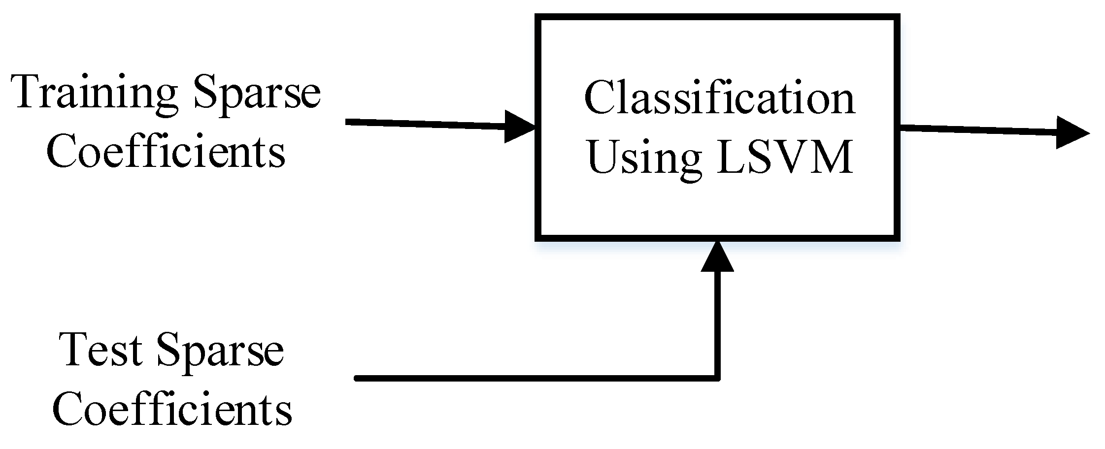
3.4. Classification by LSVM
The schematic diagram of the proposed ECG classification system is shown in Figure 3. By learning discriminative dictionary filters, it forces signals from the same class to have very similar sparse representations, so we use the LSVM for our ECG classification task. In the classification stage, each class in the training dataset contains 300 training samples, and the test dataset contains 51,722 ECG segments.
4. Experiments and Discussion
In this section, we test on the PhysioNet MIT-BIH arrhythmia database and compare the performance of the DCSC + LSVM method with other state-of-the-art classifiers.
4.1. Dataset
The proposed methodology is validated on the PhysioNet MIT-BIH Arrhythmia database [31] comprising 48 ECG records of about 30 min, sampled at 360 Hz with 11-bit resolution from 47 different patients. As recommended by the American Association of Medical Instrumentation (AAMI) [32], the MIT-BIH arrhythmia database is projected into five AAMI heartbeat classes, as described in Table 1. The ECG signal downloaded from the MIT-BIH database is processed with the help of wavelet techniques to remove baseline wander and high-frequency noise. The ECG signals sampled at 360 Hz were decomposed up to eight levels using the Bior2.6 wavelet to remove various kinds of noise [33]. The ECG would not contain much information after 45 Hz. The high-frequency noise is removed by excluding the first and second detail coefficients, which consist of bands of 90–180 Hz and 45–90 Hz. The baseline wander is removed by excluding the approximate coefficients at the fourth level. After the corresponding wavelet reconstruction, it is obvious that we can obtain a denoised ECG signal. Then, the R-peak is detected from the denoised ECG signal followed by a window across each R-peak to isolate the ECG segments for processing. After detection of the QRS complex, 99 samples preceded the QRS peak and 180 samples after the peak, and the QRS peak itself are considered as 280 samples segment as a single beat for subsequent analysis. The mapping of the MIT-BIH arrhythmia database into the AAMI recommendations along with the summary of the training and testing datasets for five classes is summarized in Table 2.
4.2. Signal Preprocessing
Roshan et al. [7,11] pointed out that through wavelet transform decomposition, the power spectral density of each type of different heartbeat has discriminative information in these two sub-bands (level 4 approximation and detail), and independent component analysis (ICA) based on wavelet transform coefficients has strong robustness and high classification accuracy. Each beat consisting of 280 samples was decomposed into four levels using the FIR approximation of Mayer’s wavelet (“dmey”). The ICA method was applied independently to the two DWT sub-bands, the fourth level approximation, and the details [7]. From each of the sub-bands fifteen ICA components were selected, so a total of thirty features from the two sub-bands were selected for subsequent pattern recognition.
4.3. Parameter Selection
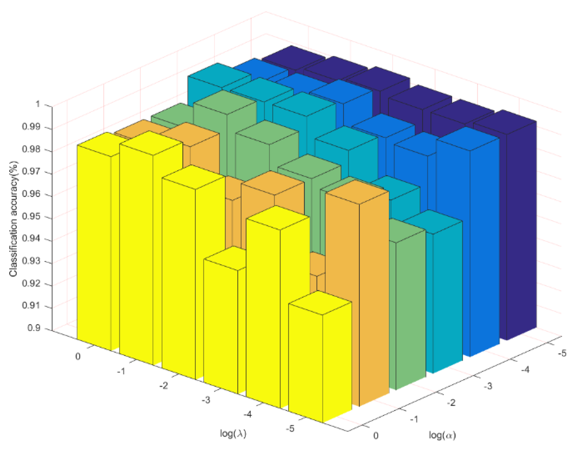
In the first set of experiments reported in Figure 4, we compare the effects of and values on classification accuracy. The and values vary from to 0. We can observe that good performance is achieved at and .
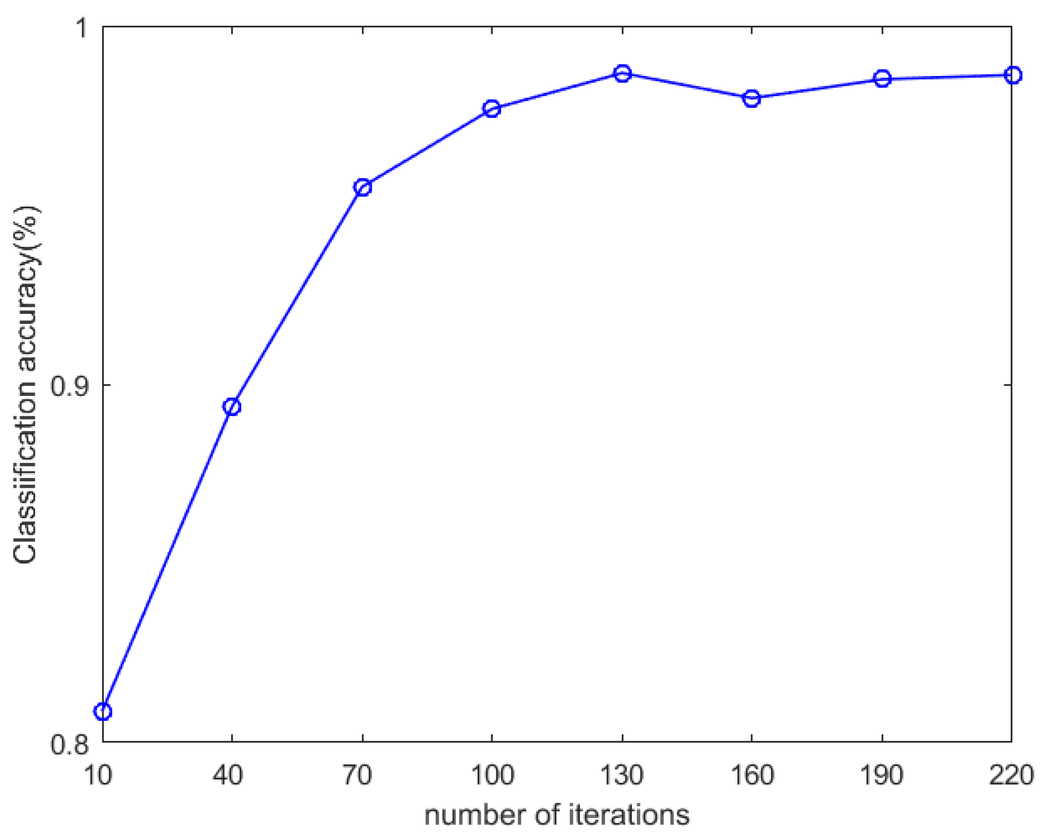
The effect of the number of iterations on the classification accuracy is shown in Figure 5. With the increase in the number of iterations, the accuracy also increases. When the number of iterations increases to 130, the accuracy rate changes very little and stabilizes to a certain value. In order to balance accuracy and complexity, the number of iterations was fixed at 130.
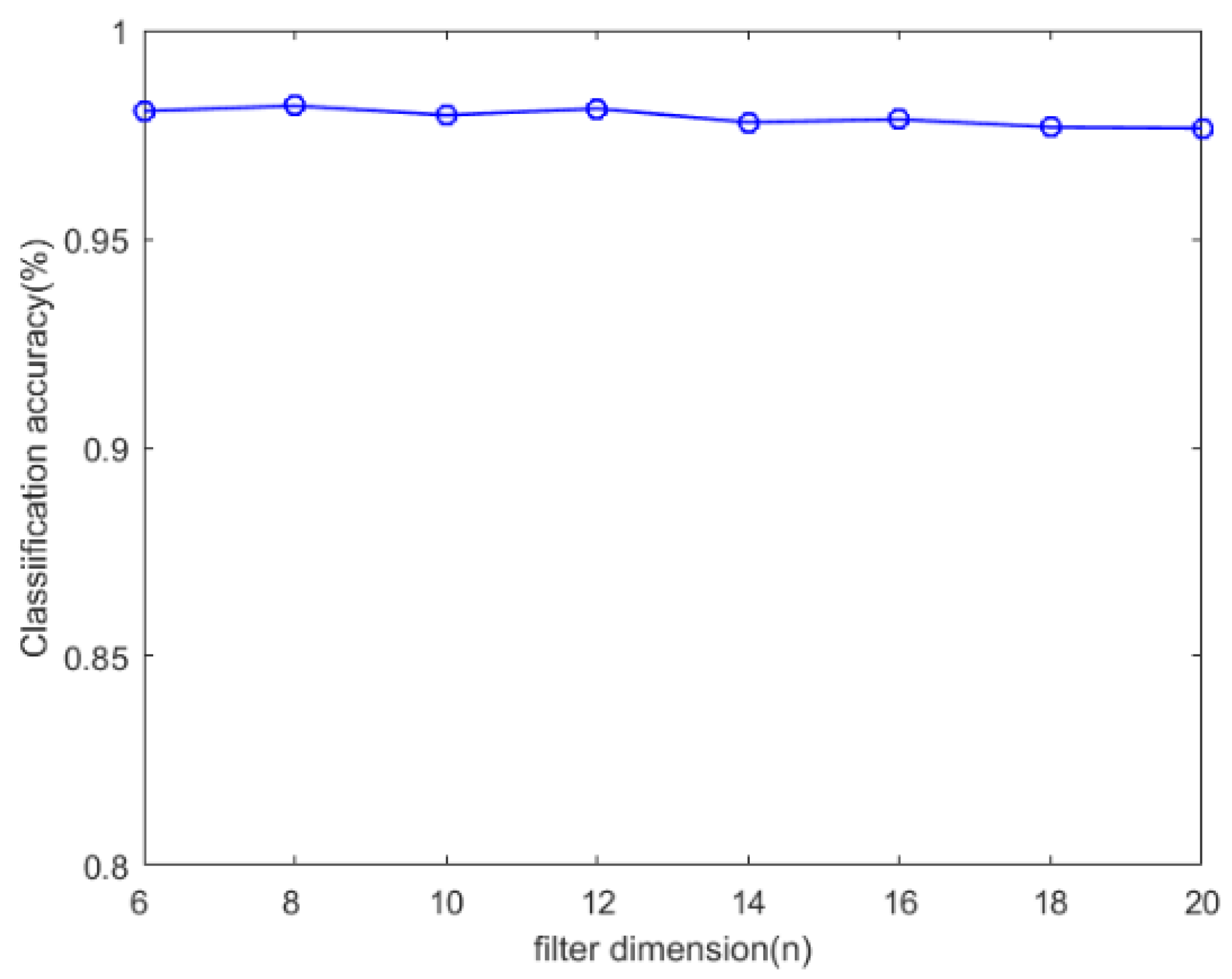
Figure 6 shows the classification accuracy when the variable dictionary filter dimension is changed from 6 to 20. In this experiment, we choose the dictionary size M = 128, and the number of training samples per class is 300. However, the overall trend is that the dictionary filter dimension has little effect on the classification performance.
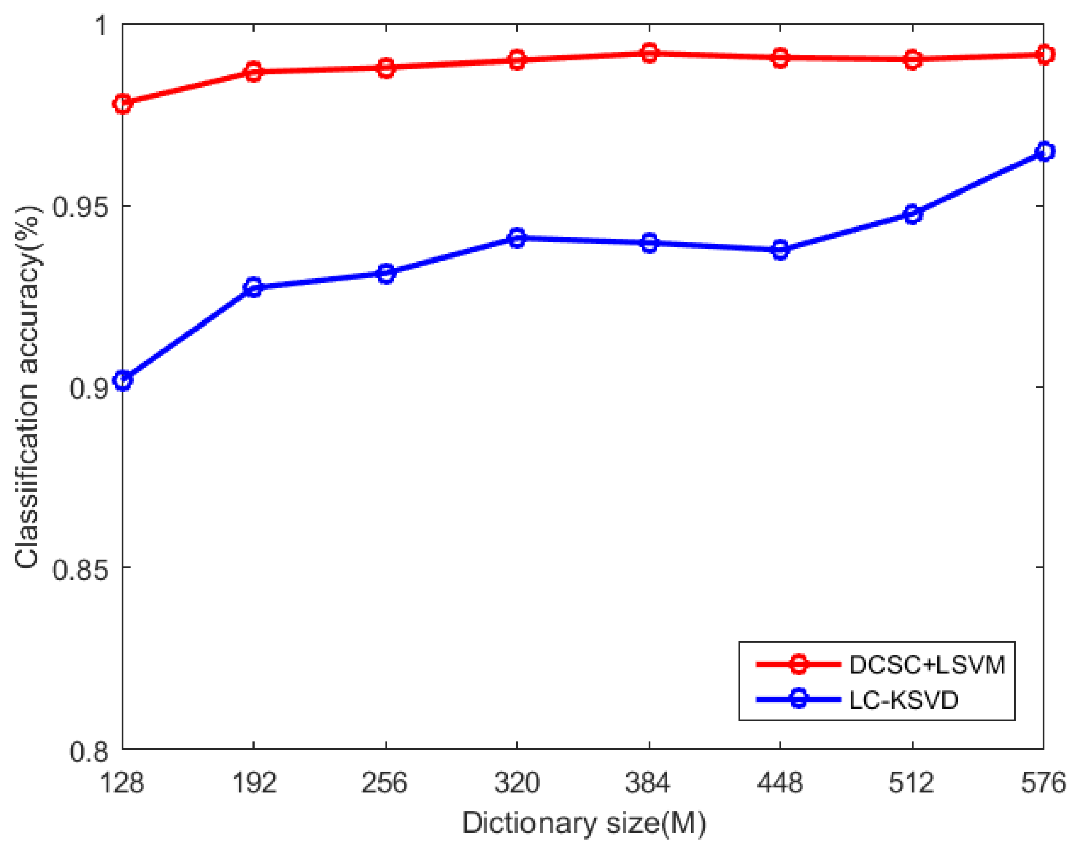
Figure 7 shows the classification results for the variable dictionary size M changing from 128 to 576. We can see that DCSC + LSVM shows an improvement of about 2.3% over LC-KSVD in all cases. In particular, even with the dictionary size M = 128, DCSC + LSVM can still have higher classification accuracy than LC-KSVD with M = 576. Moreover, from dictionary size M = 576 to M = 128, the recognition rate of DCSC + LSVM drops by 1.41%, while that of LC-KSVD drops by 6.25%. In the following classification experiments, we choose the dictionary filter dimension M = 128.
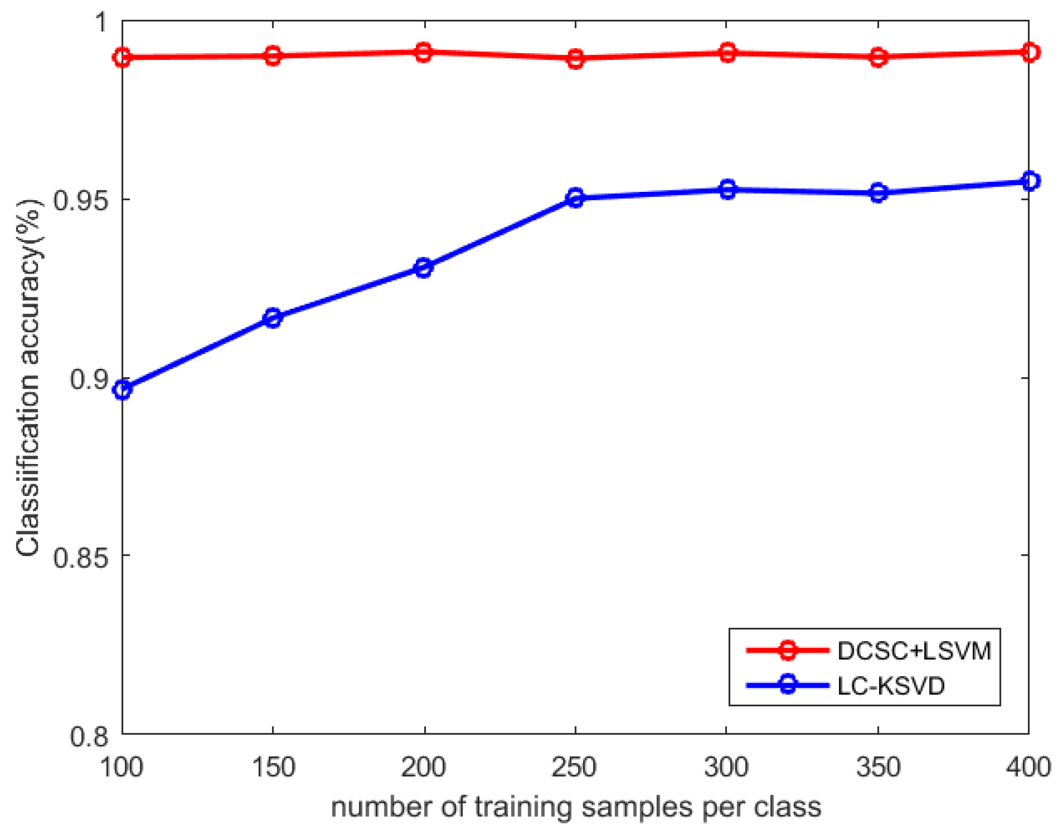
Figure 8 shows the classification results with different numbers of training samples per class. We trained 100, 150, 200, 250, 300, 350, and 400 samples per class. We can see that the different number of training samples per class has little effect on the classification performance of the DCSC + LSVM algorithm, and in all cases, the classification results of the DCSC + LSVM algorithm outperform the LC-KSVD algorithm. The classification performance of the LC-KSVD algorithm is strongly influenced by the number of training samples per class. When the number of training samples per class is less than 250, the classification results of the LC-KSVD algorithm differ from those of the DCSC + LSVM algorithm by a maximum of 9%. In the following classification experiments, we set 300 training samples per class for training.
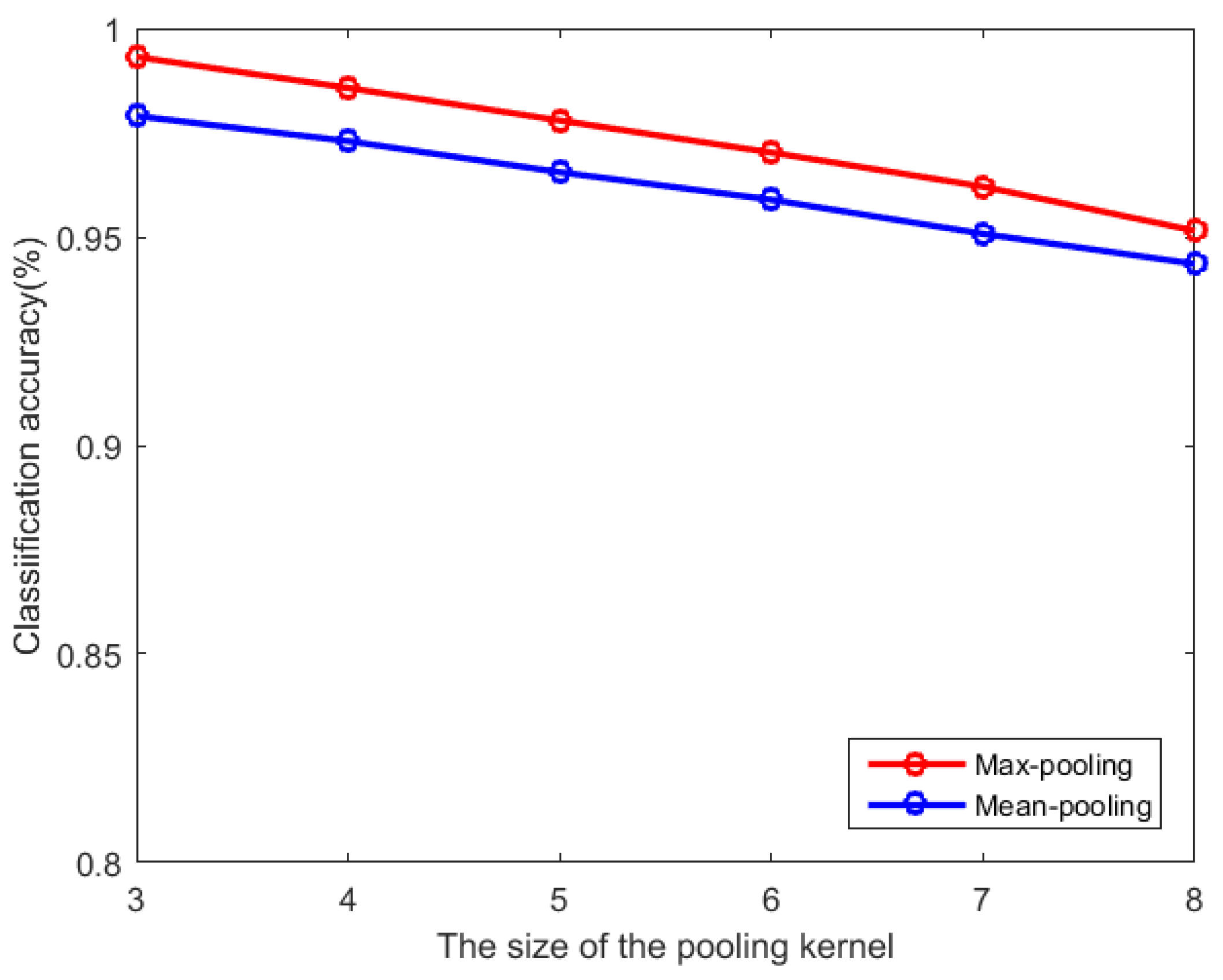
Figure 9 shows the effect of pooling kernel size on classification accuracy. In this experiment, the pooling stride is 2, and the pooling kernel is increased from 3 to 8. It can be seen from Figure 9 that with the increase of the pooling kernel, the classification accuracy decreases. At the same time, comparing the effects of max pooling and average pooling on the classification accuracy, it can be seen that the classification effect of max pooling is better than that of average pooling. So, we choose the max-pooling method, and the pooling kernel is set to 3.
4.4. Statistical Parameters
In order to analyze the performance of the classifiers, four evaluation metrics are used: sensitivity (), positive predictive value (), , and accuracy (). The , , , and can be written as
where true positive () corresponds to the number of times that the classifier correctly predicts a heartbeat without arrhythmia, i.e., normal. False positive () gives the number of arrhythmic heartbeats classified as normal. True negative () quantifies the number of heartbeats with arrhythmia that are predicted correctly. False negative () indicates the total of normal beats misclassified as arrhythmic. being defined as the harmonic mean of precision and sensitivity.
4.5. Results
We evaluated our approach on the PhysioNet MIT-BIH arrhythmia database and compared our approach with LC-KSVD [25], Fisher discrimination dictionary learning (FDDL) [24], class-specific dictionary learning (CSDL) [34], Euler label consistent KSVD (ELC-KSVD) [35], convolutional sparse coding classification (CSCC) [22], label embedded dictionary learning (LEDL) [36]. The hardware platform is Intel Xeon Gold 5122 CPU 3.60 GHz, 128.0 GB RAM, and the experimental analysis is performed by the MATLAB 2015b software package installed on the Windows 10 21H2 Microsoft USA platform. During the experiment, we also adjust the parameters of other classifiers to obtain the best classification effect. For example, in the LC-KSVD algorithm, and . In the FDDL algorithm, , . In the CSDL algorithm, . In the ELC-KSVD algorithm, , , . In the LEDL algorithm, , , and . The number of atoms per class for the FDDL, CSDL, and CSCC algorithms is the same as the number of training samples per class, which is 300. The dictionary atomic number of LC-KSVD, ELC-KSVD, and LEDL algorithms is set to 1500. The experimental results are as follows.
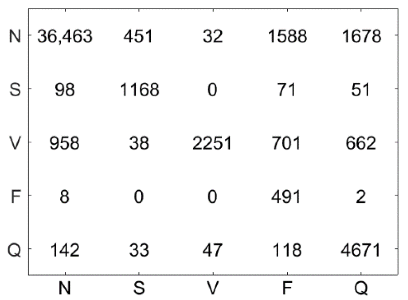
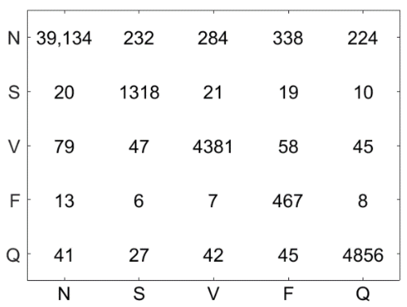
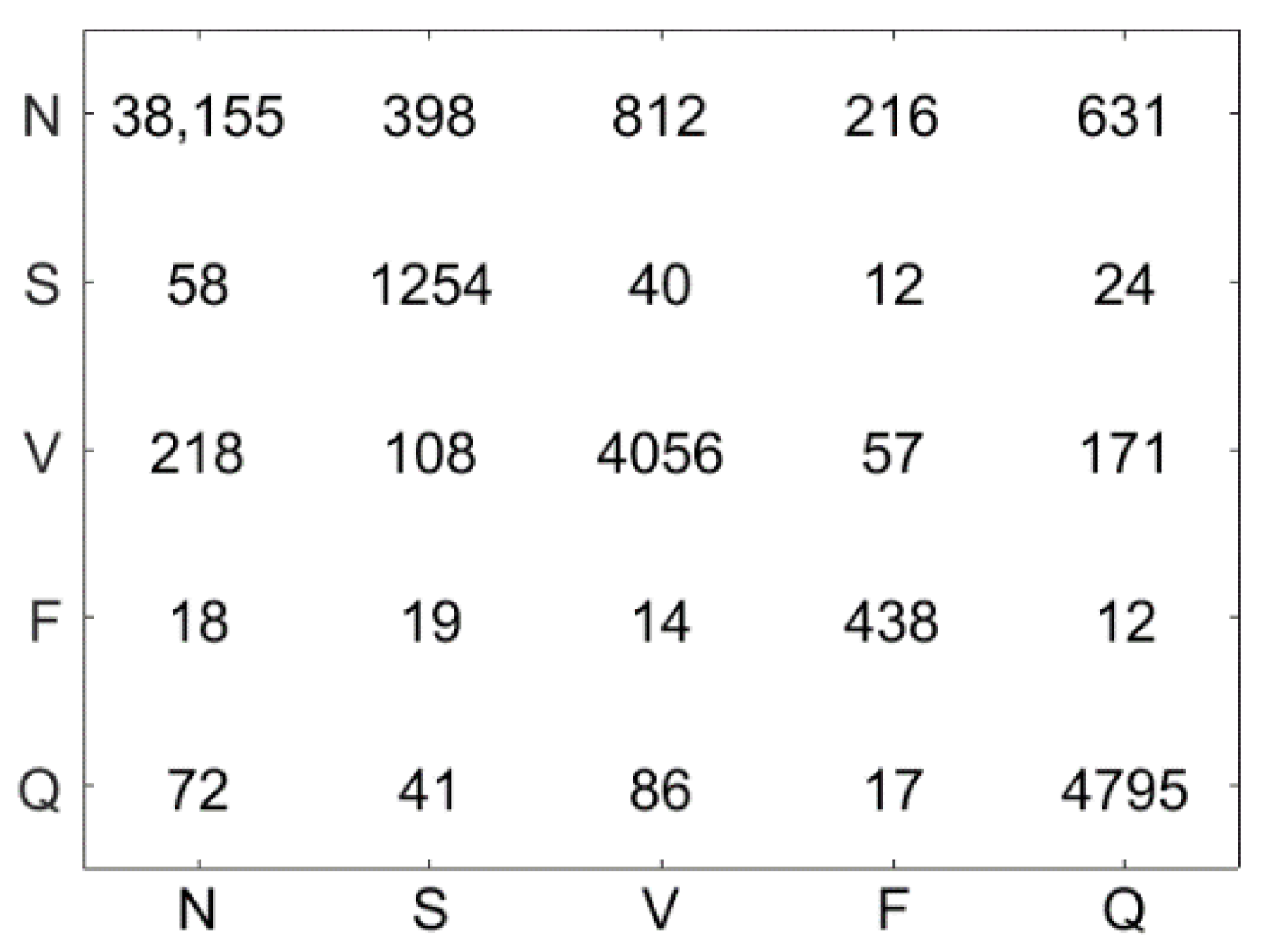
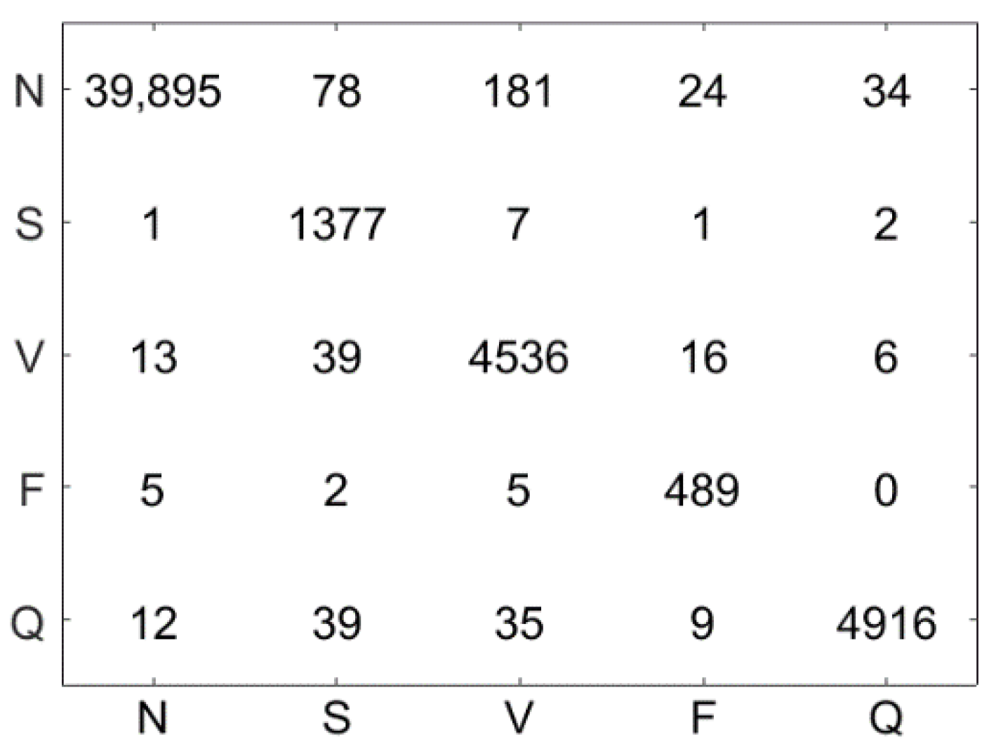
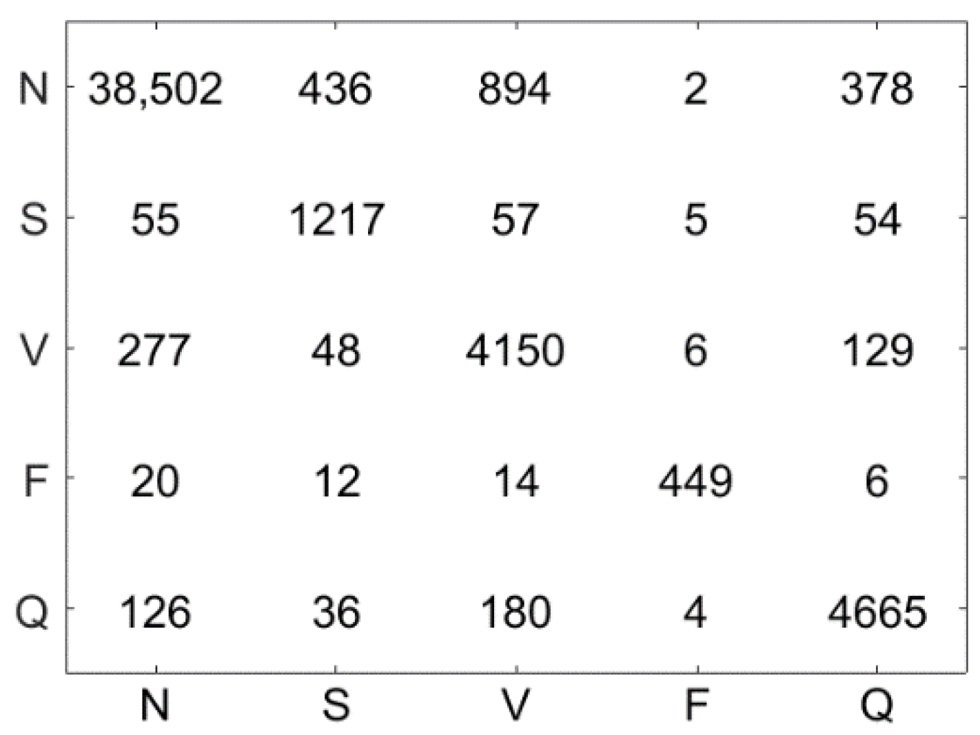
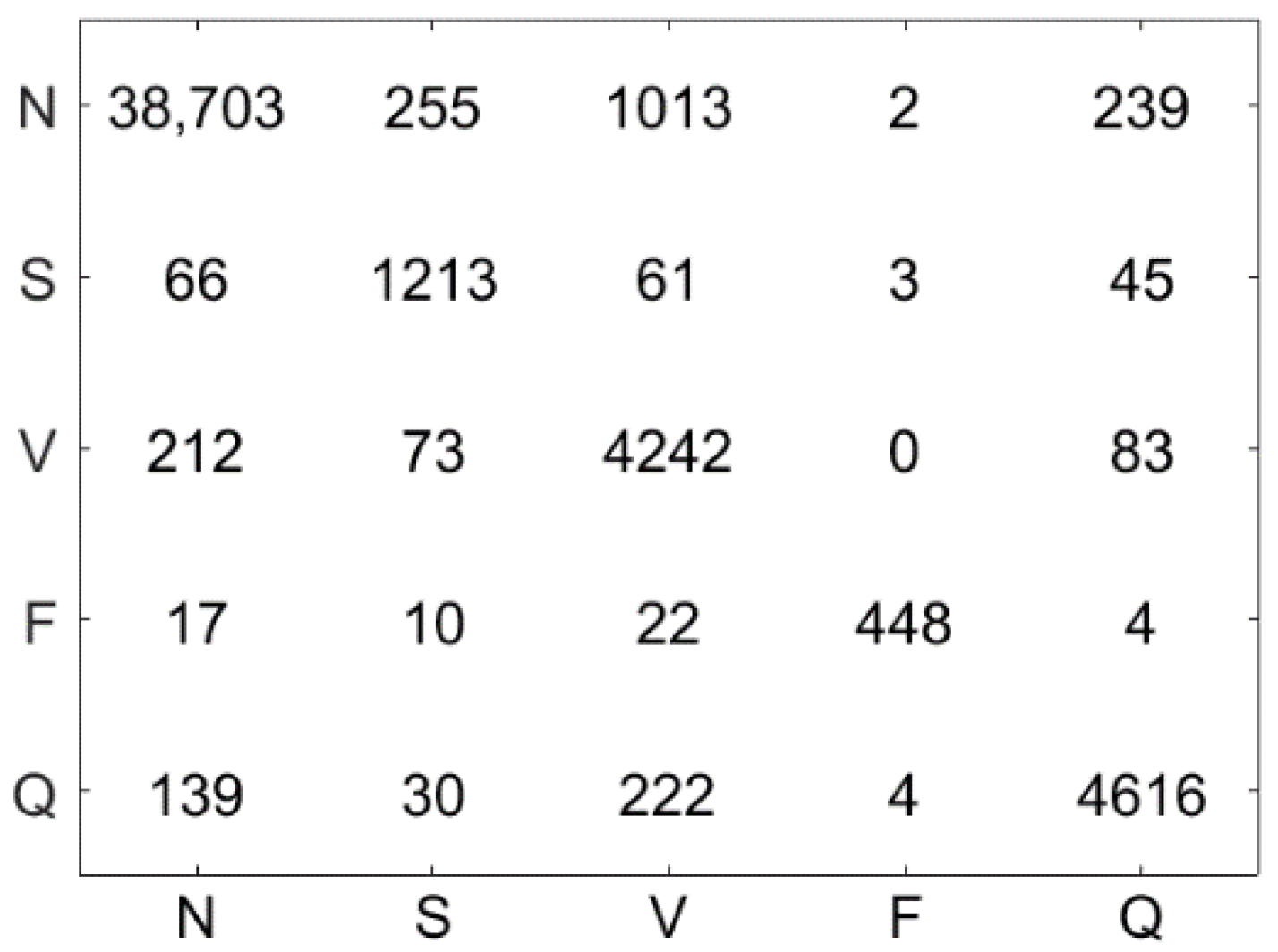
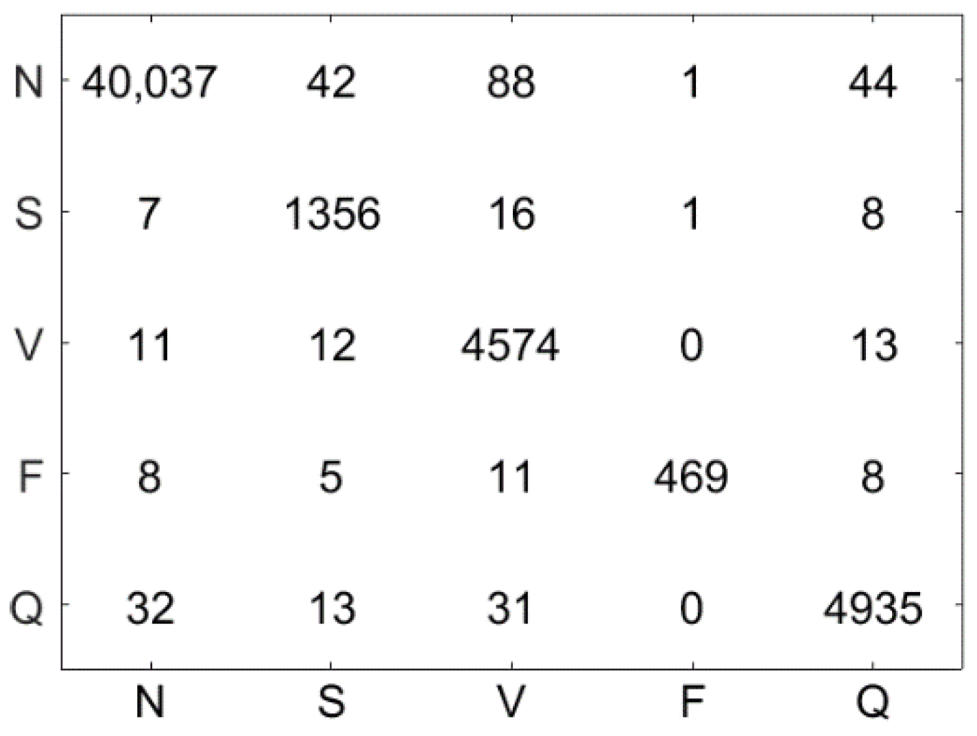
Figure 10 illustrates the confusion matrix using the LSVM method. The test dataset contains 51,722 ECG signal segments, the accuracy of the LSVM method was 87.09%, and 45,044 ECG signals were correctly classified. Figure 11 demonstrates the confusion matrix using the LC-KSVD method. The accuracy of the LC-KSVD method was 96.97%, and 50,156 ECG signals were correctly classified. Figure 12 illustrates the confusion matrix using the FDDL method. The accuracy of the FDDL method was 98.80%, and 51,100 ECG signals were correctly classified. Figure 13 illustrates the confusion matrix using the CSDL method. The accuracy of the CSDL method was 94.15%, and 48,698 ECG signals were correctly classified. Figure 14 illustrates the confusion matrix using the ELC-KSVD method. The accuracy of the ELC-KSVD method was 99.02%, and 51,213 ECG signals were correctly classified. Figure 15 illustrates the confusion matrix using the CSCC method. The accuracy of the CSCC method was 94.70%, and 48,983 ECG signals were correctly classified. Figure 16 illustrates the confusion matrix using the LEDL method. The accuracy of the LEDL method was 95.17%, and 49,222 ECG signals were correctly classified. Figure 17 illustrates the confusion matrix using the DCSC + LSVM method. The accuracy of the DCSC + LSVM method was 99.32%, and 51,371 ECG signals were correctly classified.
Table 3 shows the classification performance (, , , and ) obtained by different models on the test dataset. Compared with the LSVM algorithm, after DCSC coding, the classification accuracy is improved by 12.23%. Meanwhile, compared with LC-KSVD, FDDL, CSDL, ELC-KSVD, CSCC and LEDL, the accuracy of the proposed DCSC + LSVM is improved by 2.35%, 0.52%, 5.17%, 0.3%, 4.62%, and 4.15%, respectively. The disadvantage is that 32 S-class and 32 F-class ECG beats are misclassified. This explains why the of class S and class F are lower, and this also affects the value of class N and Q. Future efforts will look for discriminable features which get higher accuracy for classifying these beats.
In this system, to complete the classification of a segment of ECG signal, it needs to go through four stages, namely, the DWT feature extraction stage, the DCSC encoding stage, the pooling stage, and the classification stage. Since the test results of the same ECG signal were slightly different each time, we calculated the average of 10 test times as the final time. Table 4 lists the calculation time of each stage. The results show that the DCSC coding stage requires the longest computation time, the classification stage requires the shortest computation time due to the use of the linear SVM classifier, and a segment of ECG signal needs 0.336 s to complete the classification process.
4.6. Discussion
In this work, we explicitly incorporated a label consistency constraint called “discriminative sparse-code error” into the objective function of learning discriminative dictionary filters for sparse coding. The learned dictionary filters encouraged signals from the same class to have similar sparse codes, and signals from different classes to have dissimilar sparse codes. These discriminative coding coefficients allowed us to obtain good classification results even with simple linear classifiers. Compared with the LSVM algorithm, after DCSC coding, the classification accuracy is improved by 12.23%, which means that by adding label information, after DCSC coding, the coding coefficients of different classes have more obvious differences. Compared with the CSCC algorithm, the algorithm trains filter banks for each class separately but does not use the intra-class and inter-class information of the training samples during the training process, so it does not achieve good classification results. The FDDL, LC-KSVD, CSDL, ELC-KSVD, and LEDL algorithms are all supervised training algorithms and incorporate label information. The reason why their classification effect is lower than the DCSC + LSVM algorithm is that the dictionary filter bank has shift-invariance. The local features at translated positions of the sample can be extracted through the convolution operation, so a better classification effect can be obtained. We also arranged comparative experiments between DCSC + LSVM algorithm and the LC-KSVD algorithm under different dictionary sizes and different training numbers. The experimental results show that the discriminative convolutional dictionary-based learning model can obtain better classification results than LC-KSVD at a smaller dictionary size. At the same time, it is less affected by the number of training datasets. This shows that the DCSC + LSVM algorithm can be applied to a database with a small number of samples.
A comprehensive summary of the automated classification of ECG beats using the MIT-BIH arrhythmia database is shown in Table 5. Mathews et al. [7] used ICA on DWT coefficients to extract features and reported an accuracy of 99.28% using the PNN classifier. Desai et al. [37] also used ICA on DWT coefficients to extract features and obtained 98.49% accuracy using SVM quadratic kernels. Elhaj et al. [38] used PCA on DWT and ICA on HOS cumulants as features and obtained 98.91% accuracy using the SVM-RBF classifier. Acharya et al. [39] classified with an accuracy of 94.03% using a 9-layer deep convolutional neural network. Kachuee et al. [40] used a deep residual CNN network to classify with an accuracy of 93.40%. Yildirim et al. [41] used CAE and LSTM networks to classify with an accuracy of 99.00%. Romdhane et al. [42] classified with an accuracy of 98.41% using a deep CNN model and a focal loss function. Li et al. [43] used a deep residual network to classify with an accuracy of 99.06%.
The results show that the proposed model achieves higher classification accuracy compared to existing works presented in the literature and can be utilized for automated computer-aided diagnosis of several cardiovascular diseases.
5. Conclusions
In this paper, we present a novel classification model that combines the DCSC model with the LSVM classification strategy. In this work, we explicitly incorporate a label consistency constraint called “discriminative sparse-code error” into the objective function and transform the DCSC model into the Fourier domain to reduce the computational cost and optimize the DCSC model using the ADMM algorithm. By adding label information to the training phase of the convolutional dictionary filters, the learned dictionary filters encourage signals from the same class to have similar sparse codes, and signals from different classes to have dissimilar sparse codes. To reduce the computational complexity, we used a max-pooling operation for the sparse coefficients. These pooled coefficients were then used as features and fed to the LSVM classifier for the ECG classification task. The evaluation and experiments on the MIT-BIH arrhythmia database for the five classes as recommended by AAMI validate the effectiveness of the proposed DCSC + LSVM method and show that the proposed DCSC + LSVM model outperforms LSVM, LC-KSVD, FDDL, CSDL, ELC-KSVD, CSCC, LEDL and achieves state-of-the-art performance.
Author Contributions
Conceptualization, B.Z. and J.L.; methodology, B.Z. and J.L.; software, B.Z. and J.L.; validation, B.Z.; investigation, B.Z. and J.L.; writing—original draft preparation, B.Z.; writing—review and editing, B.Z. All authors have read and agreed to the published version of the manuscript.
Funding
This work was supported by the National Natural Science Foundation of China (Grant no. 61863027), the Key Research and Development Plan of Jiangxi Province (Grant no. 20202BBGL73057), the Natural Science Foundation of Jiangxi Province (Grant no. 20171BAB201013), and the Project of Nanchang Key Laboratory of Medical and Technology Research (Grant no. 2018-NCZDSY-002).
Institutional Review Board Statement
Not applicable.
Informed Consent Statement
Not applicable.
Conflicts of Interest
The authors declare that there are no conflicts of interest regarding the publication of this paper.
Appendix A. The Coding Algorithm
Using variable splitting, problem (8) in ADMM form can be reformulated as follows:
for which we have the ADMM iterations with dual variables , which are
Sub-problem Equation (A3) is solved via shrinkage/soft thresholding as
where
with and of a vector being considered to be applied element-wise and ⊙ denoting element-wise multiplication.
The most computationally expensive step is Equation (A2), which requires solving the linear system
Since is a very large matrix, it is impractical to solve this linear system using the approaches that are effective when is not a convolutional dictionary. An obvious approach is to attempt to efficiently implement convolution via the DFT convolution theorem using the Fast Fourier Transform (FFT). The variables , , , , , , and in the DFT domain are denoted by , , , , , , and , respectively. It is easy to demonstrate via the DFT convolution theorem that Equation (A7) is equivalent to
Appendix B. Convolutional form of Method of Optimal Directions
The consensus ADMM formulation of problem (11) is given as
with ADMM iterations
The problem with the update is of the form
The variables , and are denoted in the DFT domain by , , , and , respectively, where , which becomes
Defining
this problem can be expressed as
with solution
Equation (A11) is of the form
It is clear from the geometry of the problem that
or, if the normalization is desired instead
References
- Zhu, W.; Chen, X.; Wang, Y.; Wang, L. Arrhythmia recognition and classification using ECG morphology and segment feature analysis. IEEE/ACM Trans. Comput. Biol. Bioinform. 2019, 16, 131–138. [Google Scholar] [CrossRef]
- Jekova, I.; Bortolan, G.; Christov, I. Assessment and comparison of different methods for heartbeat classification. Med. Eng. Phys. 2008, 30, 248–257. [Google Scholar] [CrossRef]
- Alfaras, M.; Soriano, M.C.; Ortin, S. A fast machine learning model for ECG-Based heartbeat classification and arrhythmia detection. Front. Phys. 2019, 7, 103. [Google Scholar] [CrossRef]
- Marinho, L.B.; Nascimento, N.D.M.M.; Souza, J.W.M.; Gurgel, M.V. A novel electrocardiogram feature extraction approach for cardiac arrhythmia classification. Future Gener. Comput. Syst. 2019, 97, 564–577. [Google Scholar] [CrossRef]
- Plawiak, P. Novel methodology of cardiac health recognition based on ECG signals and evolutionary-neural system. Expert Syst. Appl. 2018, 92, 334–349. [Google Scholar] [CrossRef]
- Aziz, S.; Ahmed, S.; Alouini, M. ECG-based machine learning algorithms for heartbeat classification. Sci. Rep. 2021, 11, 18738. [Google Scholar] [CrossRef]
- Martis, R.J.; Acharya, U.R.; Min, L.C. ECG beat classification using PCA, LDA, ICA and discrete wavelet transform. Biomed. Signal Proces. 2013, 85, 437–448. [Google Scholar] [CrossRef]
- Minhas, F.A.; Arif, M. Robust electrocardiogram (ECG) beat classification using discrete wavelet transform. Physiol. Meas. 2008, 29, 555–570. [Google Scholar] [CrossRef]
- Martis, R.J.; Chakraborty, C.; Ray, A.K. An integrated ECG feature extraction scheme using PCA and wavelet transform. In Proceedings of the 2009 Annual IEEE India Conference, Ahmedabad, India, 18–20 December 2009; p. 422. [Google Scholar]
- Lin, C. Frequency-domain features for ECG beat discrimination using grey relational analysis-based classifier. Comput. Math. Appl. 2008, 55, 680–690. [Google Scholar] [CrossRef]
- Martis, R.J.; Acharya, U.R.; Mandana, K.M.; Ray, A.K. Application of principal component analysis to ECG signals for automated diagnosis of cardiac health. Expert Syst. Appl. 2012, 39, 11792–11800. [Google Scholar] [CrossRef]
- Wan, M.; Lai, Z.; Yang, G.; Yang, Z. Local graph embedding based on maximum margin criterion via fuzzy set. Fuzzy Set. Syst. 2017, 318, 120–131. [Google Scholar] [CrossRef]
- Wan, M.; Chen, X.; Zhan, T.; Xu, C. Sparse Fuzzy Two-Dimensional Discriminant Local Preserving Projection (SF2DDLPP) for Robust Image Feature Extraction. Inform. Sci. 2021, 563, 1–15. [Google Scholar] [CrossRef]
- Hammad, M.; Maher, A.; Wang, K.; Jiang, F. Detection of abnormal heart conditions based on characteristics of ECG signals. Measurement 2018, 125, 634–644. [Google Scholar] [CrossRef]
- Matta, S.C.; Sankari, Z.; Rihana, S. Heart rate variability analysis using neural network models for automatic detection of lifestyle activities. Biomed. Signal Process 2018, 42, 145–157. [Google Scholar] [CrossRef]
- Heide, F.; Heidrich, W.; Wetzstein, G. Fast and flexible convolutional sparse coding. In Proceedings of the IEEE Conference on Computer Vision and Pattern Recognition (CVPR), Boston, MA, USA, 7–12 June 2015; pp. 5135–5143. [Google Scholar]
- Papyan, V.; Romano, Y.; Sulam, J.; Elad, M. Convolutional dictionary learning via local processing. In Proceedings of the 16th IEEE International Conference on Computer Vision (ICCV), Venice, Italy, 22–29 October 2017; pp. 5306–5314. [Google Scholar]
- Liu, Y.; Chen, X.; Ward, R.K.; Wang, Z.J. Image fusion with convolutional sparse representation. IEEE Signal Proc. Let. 2016, 23, 1882–1886. [Google Scholar] [CrossRef]
- Zeiler, M.D.; Taylor, G.W.; Fergus, R. Adaptive deconvolutional networks for mid and high level feature learning. In Proceedings of the IEEE International Conference on Computer Vision (ICCV), Washington, DC, USA, 6–13 November 2011; pp. 2018–2025. [Google Scholar]
- Sermanet, P.; Kavukcuoglu, K.; Chintala, S.; LeCun, Y. Pedestrian detection with unsupervised multistage feature learning. In Proceedings of the 26th IEEE Conference on Computer Vision and Pattern Recognition (CVPR), Portland, OR, USA, 23–28 June 2013; pp. 3626–3633. [Google Scholar]
- Zhou, Y.; Chang, H.; Barner, K.; Spellman, P. Classification of histology sections via multispectral convolutional sparse coding. In Proceedings of the 27th IEEE Conference on Computer Vision and Pattern Recognition (CVPR), Columbus, OH, USA, 23–28 June 2014; pp. 3081–3088. [Google Scholar]
- Chen, B.; Li, J.; Ma, B.; Wei, G. Convolutional sparse coding classification model for image classification. In Proceedings of the IEEE International Conference on Image Processing ICIP, Phoenix, AZ, USA, 25–28 September 2016; pp. 1918–1922. [Google Scholar]
- Zhang, Q.; Li, B. Discriminative K-SVD for dictionary learning in face recognition. In Proceedings of the 23rd IEEE Conference on Computer Vision and Pattern Recognition (CVPR), Portland, OR, USA, 23–28 June 2010; pp. 2691–2698. [Google Scholar]
- Yang, M.; Zhang, L.; Feng, X.; Zhang, D. Fisher discrimination dictionary learning for sparse representation. In Proceedings of the IEEE International Conference on Computer Vision (ICCV), Barcelona, Spain, 6–13 November 2011; pp. 543–550. [Google Scholar]
- Jiang, Z.L.; Lin, Z.; Davis, L.S. Label consistent K-SVD: Learning a discriminative dictionary for recognition. IEEE Trans. Pattern Anal. 2013, 35, 2651–2664. [Google Scholar] [CrossRef] [PubMed]
- Wohlberg, B. Efficient algorithms for convolutional sparse representations. IEEE T Image Process. 2016, 25, 301–315. [Google Scholar] [CrossRef]
- Boyd, S.; Parikh, N.; Chu, E.; Peleato, B. Distributed optimization and statistical learning via the alternating direction method of multipliers. Found. Trends Mach. Learn. 2010, 3, 1–122. [Google Scholar] [CrossRef]
- Garcia-Cardona, C.; Wohlberg, B. Convolutional dictionary learning: A comparative review and new algorithms. IEEE Trans. Comput. Imag. 2018, 4, 366–381. [Google Scholar] [CrossRef]
- Zubair, S.; Yan, F.; Wang, W. Dictionary learning based sparse coefficients for audio classification with max and average pooling. Digit. Signal Process. 2013, 23, 960–970. [Google Scholar] [CrossRef]
- Wang, J.; Yang, J.; Yu, K.; Lv, F. Locality-constrained linear coding for image classification. In Proceedings of the 23rd IEEE Conference on Computer Vision and Pattern Recognition (CVPR), San Francisco, CA, USA, 13–18 June 2010; pp. 3360–3367. [Google Scholar]
- Moody, G.; Mark, R. The impact of the MIT-BIH arrhythmia database. IEEE Eng. Med. Biol. 2001, 20, 45–50. [Google Scholar] [CrossRef] [PubMed]
- ANSI/AAMI EC57:1998; Testing and Reporting Performance Results of Cardiac Rhythm and ST Segment Measurement Algorithms. Association for the Advancement of Medical Instrumentation: American National Standards Institute, Inc. (ANSI): Washington, DC, USA, 1998.
- Singh, B.N.; Tiwari, A.K. Optimal selection of wavelet basis function applied to ECG signal denoising. Digit. Signal Process. 2006, 16, 275–287. [Google Scholar] [CrossRef]
- Liu, B.D.; Shen, B.; Gui, L. Face recognition using class Specific dictionary learning for sparse representation and collaborative representation. Neurocomputing 2016, 204, 198–210. [Google Scholar] [CrossRef]
- Song, Y.; Liu, Y.; Gao, Q.; Gao, X. Euler label consistent k-svd for image classification and action recognition. Neurocomputing 2018, 310, 277–286. [Google Scholar] [CrossRef]
- Shao, S.; Xu, R.; Liu, W.; Liu, B. Label embedded dictionary learning for image classification. Neurocomputing 2020, 385, 122–131. [Google Scholar] [CrossRef]
- Desai, U.; Martis, R.J.; Nayak, C.G.; Sarika, K. Machine intelligent diagnosis of ECG for arrhythmia classification using DWT, ICA and SVM techniques. In Proceedings of the 12 IEEE International Conference on Elect Energy Env Communications Computer Control, New Delhi, India, 17–20 December 2015; p. 2015. [Google Scholar]
- Elhaj, F.A.; Salim, N.; Harris, A.R.; Swee, T.T. Arrhythmia recognition and classification using combined linear and nonlinear features of ECG signals. Comput. Method Prog. Biomed. 2016, 127, 52–63. [Google Scholar] [CrossRef]
- Acharya, U.R.; Oh, S.L.; Hagiwara, Y. A deep convolutional neural network model to classify heartbeats. Comput. Biol. Med. 2017, 89, 389–396. [Google Scholar] [CrossRef]
- Mohammad, K.; Shayan, F.; Majid, S. ECG heartbeat classification: A deep transferable representation. In Proceedings of the International Conference Healthcare Informativa ICHI, New York, NY, USA, 4–7 June 2018; pp. 443–444. [Google Scholar]
- Yildirim, O.; Baloglu, U.B.; Tan, R. A new approach for arrhythmia classification using deep coded features and LSTM networks. Comput. Method Prog. Biomed. 2019, 176, 121–133. [Google Scholar] [CrossRef]
- Romdhane, T.F.; Alhichri, H.; Ouni, R.; Atri, M. Electrocardiogram heartbeat classification based on a deep convolutional neural network and focal loss. Comput. Biol. Med. 2020, 123, 103866. [Google Scholar] [CrossRef]
- Li, Z.; Zhou, D.; Wan, L.; Li, J. Heartbeat classification using deep residual convolutional neural network from 2-lead electrocardiogram. J. Electrocardiol. 2020, 58, 105–112. [Google Scholar] [CrossRef]
Figure 1.
Block diagram of the proposed ECG classification system.

Figure 2.
Extraction of sparse coefficients using convolutional sparse coding.

Figure 3.
ECG classification using LSVM.

Figure 4.
Effects of and parameter selection on classification accuracy.

Figure 5.
The effect of the number of iterations on the classification accuracy.

Figure 6.
Classification accuracy based on variable dictionary filter dimension.

Figure 7.
Classification accuracy based on variable dictionary size M.

Figure 8.
Classification accuracy based on different numbers of training samples per class.

Figure 9.
Effects of the Pooling Kernel Size on the Classification Accuracy.

Figure 10.
Confusion matrix using the LSVM model.

Figure 11.
Confusion matrix using the LC-KSVD model.

Figure 12.
Confusion matrix using the FDDL model.

Figure 13.
Confusion matrix using the CSDL model.

Figure 14.
Confusion matrix using the ELC-KSVD model.

Figure 15.
Confusion matrix using the CSCC model.

Figure 16.
Confusion matrix using the LEDL model.

Figure 17.
Confusion matrix using the DCSC + LSVM model.


Table 1.
Heartbeats of the MIT-BIH arrhythmia database classified based on the ANSI/AAMI EC57:1998 standard.
Table 1.
Heartbeats of the MIT-BIH arrhythmia database classified based on the ANSI/AAMI EC57:1998 standard.
| N | S | V | F | Q |
|---|---|---|---|---|
|
|
|
|
|
|
Table 2.
A summary of the 5 classes of beat subtypes.
| AAMI Classes | Training Data | Testing Data | Total Data |
|---|---|---|---|
| N | 300 | 40,212 | 40,512 |
| S | 300 | 1388 | 1688 |
| V | 300 | 4610 | 4910 |
| F | 300 | 501 | 801 |
| Q | 300 | 5011 | 5311 |
| Total | 1500 | 51,722 | 53,222 |
Table 3.
Performance metrics of different algorithms.
| Method | N | S | V | F | Q | |||||||||||
|---|---|---|---|---|---|---|---|---|---|---|---|---|---|---|---|---|
| % | ||||||||||||||||
| LSVM | 87.09 | 90.68 | 96.80 | 93.64 | 84.15 | 69.11 | 75.89 | 48.83 | 96.61 | 64.87 | 98.00 | 16.54 | 28.30 | 93.21 | 66.12 | 77.37 |
| LC-KSVD | 96.97 | 97.32 | 99.61 | 98.45 | 94.96 | 80.86 | 87.34 | 95.03 | 92.52 | 93.76 | 93.21 | 50.38 | 65.41 | 96.91 | 94.42 | 95.65 |
| FDDL | 98.80 | 98.93 | 99.92 | 99.42 | 99.35 | 90.37 | 94.65 | 99.15 | 93.67 | 96.33 | 98.80 | 91.67 | 95.10 | 97.27 | 98.19 | 97.72 |
| CSDL | 94.15 | 94.88 | 99.05 | 96.92 | 90.35 | 68.90 | 78.18 | 87.98 | 80.99 | 84.34 | 87.43 | 59.19 | 70.59 | 95.69 | 85.12 | 90.10 |
| ELC-KSVD | 99.02 | 99.21 | 99.92 | 99.57 | 99.21 | 89.71 | 94.22 | 98.39 | 95.21 | 96.78 | 97.60 | 90.72 | 94.04 | 98.10 | 99.15 | 98.63 |
| CSCC | 94.70 | 95.75 | 98.77 | 97.24 | 87.68 | 69.58 | 77.59 | 90.02 | 78.38 | 83.80 | 89.62 | 96.35 | 92.86 | 93.10 | 89.16 | 91.09 |
| LEDL | 95.17 | 96.25 | 98.89 | 97.55 | 87.39 | 76.72 | 81.71 | 92.02 | 76.29 | 83.42 | 89.42 | 98.03 | 93.53 | 92.12 | 92.56 | 92.34 |
| DCSC + LSVM | 99.32 | 99.56 | 99.86 | 99.71 | 97.69 | 94.96 | 96.31 | 99.22 | 96.91 | 98.05 | 93.61 | 99.58 | 96.50 | 98.48 | 98.54 | 98.51 |
Table 4.
Computation time for each stage for a test sample.
| Methods | DWT + ICA | DCSC | Pooling | Classification |
|---|---|---|---|---|
| Time(s) | 0.058 | 0.198 | 0.078 | 0.002 |
Table 5.
Comparison of works on ECG heartbeat classification from MIT-BIH.
| Literature | Features | Classifier | Classes | |
|---|---|---|---|---|
| Mathews et al. [7] | DWT + ICA | PNN | 5 | 99.28 |
| Desai et al. [37] | DWT + ICA | SVM quadratic kernel | 5 | 98.49 |
| Elhaj et al. [38] | PCA + DWT + HOS + ICA | SVM-RBF | 5 | 98.91 |
| Acharya et al. [39] | 9-layer deep convolutional neural network | 5 | 94.03 | |
| M. Kachuee et al. [40] | deep residual CNN | 5 | 93.40 | |
| Yildirim et al. [41] | CAE and LSTM | 5 | 99.00 | |
| Romdhane et al. [42] | Deep CNN | 5 | 98.41 | |
| Li et al. [43] | Deep residual network | 5 | 99.06 | |
| Proposed | DWT + ICA | DCSC + LSVM | 5 | 99.32 |
Publisher’s Note: MDPI stays neutral with regard to jurisdictional claims in published maps and institutional affiliations. |
© 2022 by the authors. Licensee MDPI, Basel, Switzerland. This article is an open access article distributed under the terms and conditions of the Creative Commons Attribution (CC BY) license (https://creativecommons.org/licenses/by/4.0/).
Share and Cite
MDPI and ACS Style
Zhang, B.; Liu, J. Discriminative Convolutional Sparse Coding of ECG Signals for Automated Recognition of Cardiac Arrhythmias. Mathematics 2022, 10, 2874. https://0-doi-org.brum.beds.ac.uk/10.3390/math10162874
AMA Style
Zhang B, Liu J. Discriminative Convolutional Sparse Coding of ECG Signals for Automated Recognition of Cardiac Arrhythmias. Mathematics. 2022; 10(16):2874. https://0-doi-org.brum.beds.ac.uk/10.3390/math10162874
Chicago/Turabian StyleZhang, Bing, and Jizhong Liu. 2022. "Discriminative Convolutional Sparse Coding of ECG Signals for Automated Recognition of Cardiac Arrhythmias" Mathematics 10, no. 16: 2874. https://0-doi-org.brum.beds.ac.uk/10.3390/math10162874
Note that from the first issue of 2016, this journal uses article numbers instead of page numbers. See further details here.