
Language Accent Detection with CNN Using Sparse Data from a Crowd-Sourced Speech Archive

 , , , ,
  and
and
Abstract
:1. Introduction
- Analysis and modeling of speakers’ variability in frame of speech recognition [9];
- Development of user interaction scenarios in video-games [11];
- Analysis of phonetic particularities and related personal behavior [12];
- Using accent-related information as components of biometric data [13];
- Mitigating accent influence in voice-control systems [14];
- Improving personalization of exercises and feedback in CAPT systems [2].
2. Scope of Research
3. Materials, Methods and Tools
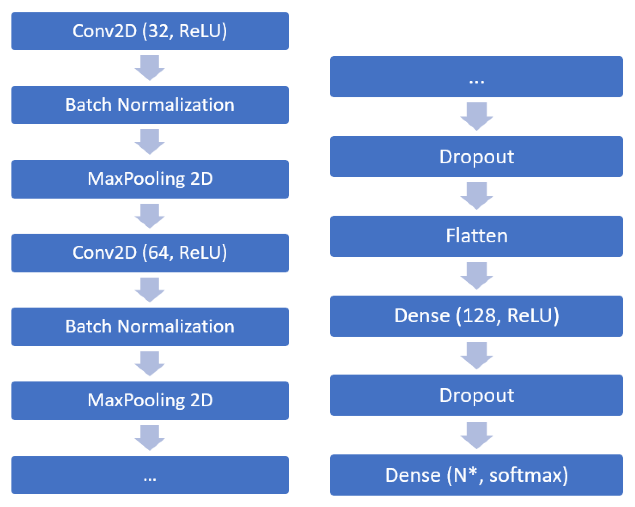
3.1. Adopting the CNN Model to Speech Signal Processing
3.2. Data Collection
“Please call Stella. Ask her to bring these things with her from the store: Six spoons of fresh snow peas, five thick slabs of blue cheese, and maybe a snack for her brother Bob. We also need a small plastic snake and a big toy frog for the kids. She can scoop these things into three red bags, and we will go meet her Wednesday at the train station.”
- Speaker diversity assuring an adequate representation of different varieties of pronunciation;
- Uniformity of material referring to the same content and context;
- Phonetic balance when individual phonemes do not occur too often;
- Presence of a semantic load of sentences avoiding semantic factors that might affect pronunciation [17];
- Working with speech segments rather than independent words.
3.2.1. Data Classes (L1 Languages)
3.2.2. Preparing Audio Files for Recognition
3.2.3. Fragments of Silence
3.3. Feature Selection
- Spectral centroid (SC) represents “center of mass” of the input sound, which formally corresponds to the frequency at which the energy of the spectrum is concentrated:being the value of the frame signal spectrum t of the frequency interval n, Hz.
- Spectral rolloff (SR) is a measure of the asymmetry of the spectral shape of the signal. It represents the frequency , such as a given percentage (usually 85%) of the total energy of the spectrum that lies below . In order to calculate this value, one needs to find the proportion of frames in the signal power spectrum, where a given percentage of power falls on lower frequencies. Thus, the spectral rolloff is a frequency such as:where is the value of the frame signal spectrum t of the frequency interval n, Hz. This value is used to determine vocalized sounds in speech, since the unvoiced sounds have a large proportion of the energy contained in the high frequency range of the spectrum.
- Chromagram is usually a 12-dimensional feature vector representing the amount of energy for each of the signal’s height classes (such as C, C#, D, D#, E, etc.).
- Zero Crossing (ZCR) represents the number of signal sign changes within a segment. The ZCR feature can be helpful in describing the signal noisiness:where is a signal of duration t, is a characteristic function whose value is equal to 1 if condition X is satisfied and 0, otherwise. For unvoiced speech, the ZCR characteristic takes on higher values.
- Root mean square (RMS) is a standard measure representing the average signal strength:Calculating RMS directly from the audio recordings is faster because it does not require calculating STFT. However, using a spectrogram can give a more accurate representation of signal energy over time because its frames can be split into windows. Since the characteristics of the signal can be stored in an external file in advance (before training the model), decreasing the extraction time was not critical. That is why, in our case, to improve the signal representation accuracy, RMS was calculated based on the signal spectrogram.
- Fundamental frequency () is the lowest frequency of the periodic signal. is the frequency at which a person’s vocal cords vibrate while producing the voiced sounds. The fundamental frequency carries a lot of information about the pitch of the voice at any given time, and therefore, about the overall intonation of the speech. It has been studied that makes a significant contribution to the perception of foreign accents [6], which is especially noticeable for Germanic and Romance languages [32]. An estimation of the fundamental frequency of the signal has been carried out using the autocorrelation-based YIN algorithm [33]. According to this algorithm, initially, a cumulative mean normalized difference function is computed for short overlapped audio fragments. Then, the smallest lag giving the minimum of the normalized difference function below the threshold is chosen as the period estimate of the signal. Finally, the period estimate before converting to the corresponding frequency is refined using parabolic interpolation. Since there is no upper limit to the frequency search range for YIN, this algorithm is also suitable for higher voices. In addition, YIN is a relatively simple algorithm that can be implemented efficiently with low latency, and requires few parameters to be tuned.
3.4. Batch Normalization
3.5. Classification Model
4. Experiments and Results
4.1. CNN Model Tuning and Data Augmentation
4.2. Input Acoustic Feature Sets
4.2.1. Dimension of Input
4.2.2. MFCC Combined with Additional Features
4.2.3. Mel-Spectograms
5. Evaluation
6. Discussion
7. Conclusions
- Using additional audio signal information on time–frequency and energy features (such as spectrogram, chromogram, spectral centroid, spectral rolloff, and fundamental frequency), mel-frequency cepstral coefficients (MFCC) are proven to increase the accuracy of the accent classification compared to a conventional feature set based on MFCC and raw spectrograms.
- Amplitude mel-spectrograms on a linear scale (in contrast to logarithmic scale used in most studies) appear more powerful in the accent classification task and make it possible to produce state-of-the-art accent recognition accuracy, ranging from 0.964 to 0.987.
- Reported accuracy has been achieved using heterogeneous sparse data from the Speech Accent Archive, unlike the best reported experiments, where the datasets are prepared in standardized conditions using the same equipment. This outcome addresses real life situations, with varying recording environments and tools.
- Based on our experiments, we demonstrated that the pauses in speech have a positive effect on the ability to determine accents. This is why they should not be eliminated from the input, at least with respect to the accent classification process.
- The experiments conducted enhanced our understanding of how intonation may impact accent recognition. Based on the fact that the fundamental frequency contour in most experiments did not improve the classification results, we concluded that intonation features are subsumed within MFCC. To the best of our knowledge, the problem of accent recognition in connection to the analysis of language prosody features makes an important and additional novel contribution.
Author Contributions
Funding
Institutional Review Board Statement
Informed Consent Statement
Data Availability Statement
Conflicts of Interest
Abbreviations
| ASR | Automatic Speech Recognition |
| bLSTM | Bidirectional Long Short-term Model |
| CAPT | Computer-assisted Pronunciation Training |
| CG | Chromagram |
| CNN | Convolutional Neural Networks |
| FFNN | Feedforward Neural Network |
| GMM | Gaussian Mixture Model |
| HMM | Hidden Markov Model |
| IR | Information Retrieval |
| KNN | k-nearest Neighbor |
| LSTM | Long Short-term Model |
| MDPI | Multidisciplinary Digital Publishing Institute |
| MFCC | Mel-frequency Cepstral Coefficients |
| RF | Random Forest |
| RMS | Root Mean Square |
| SC | Spectral Centroid |
| SFF | Single Filtered Frequency |
| SG | Spectrogram |
| STFT | Short-time Fourier Transform |
| SVM | Support Vector Machine |
| SR | Spectral Rolloff |
| ZCR | Zero CRossing |
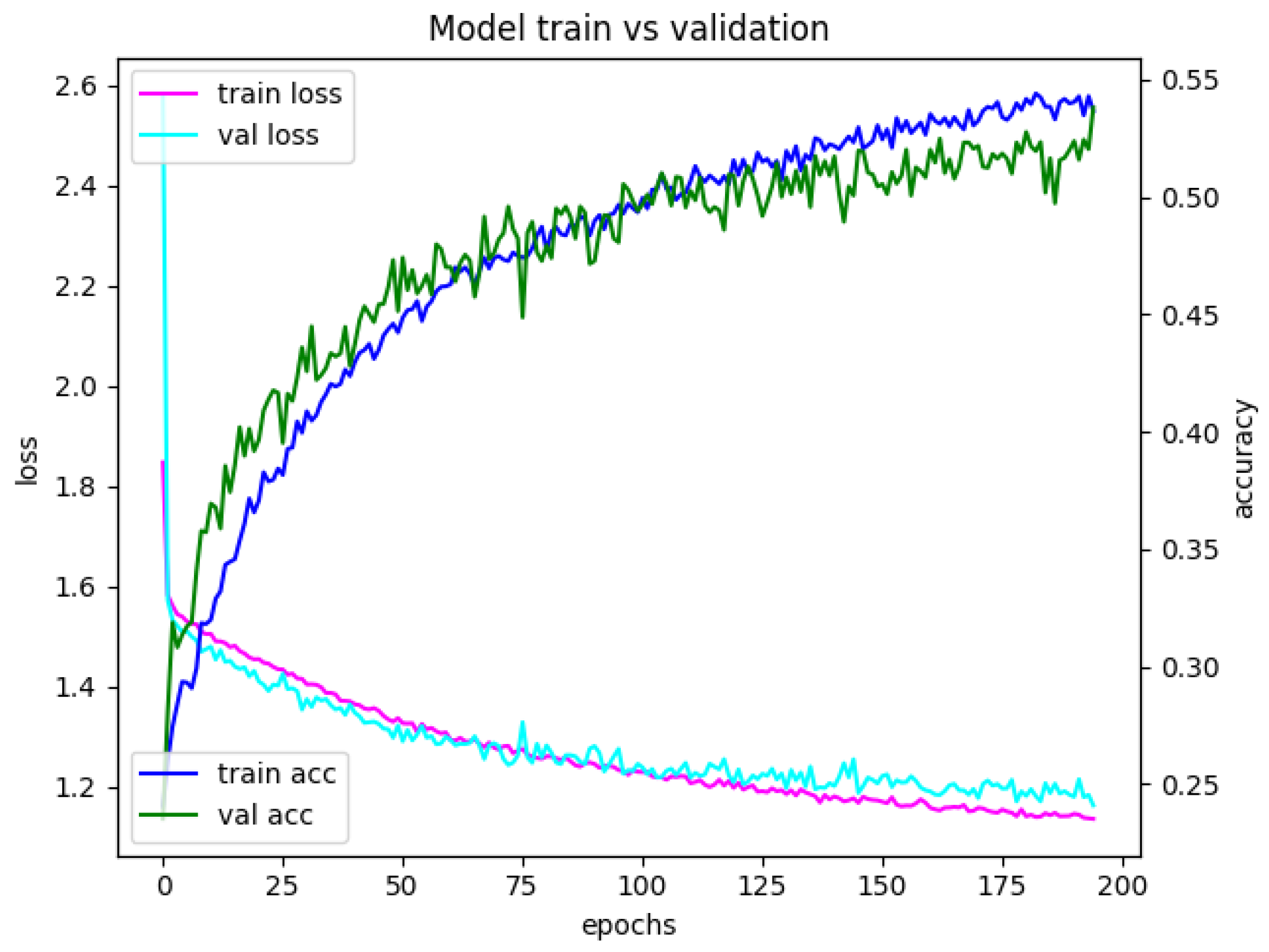
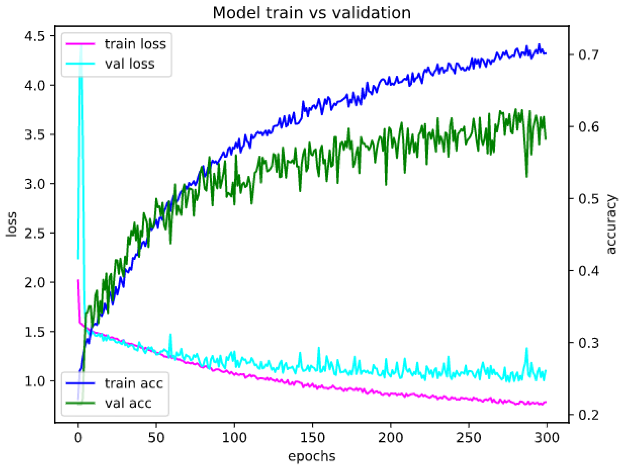
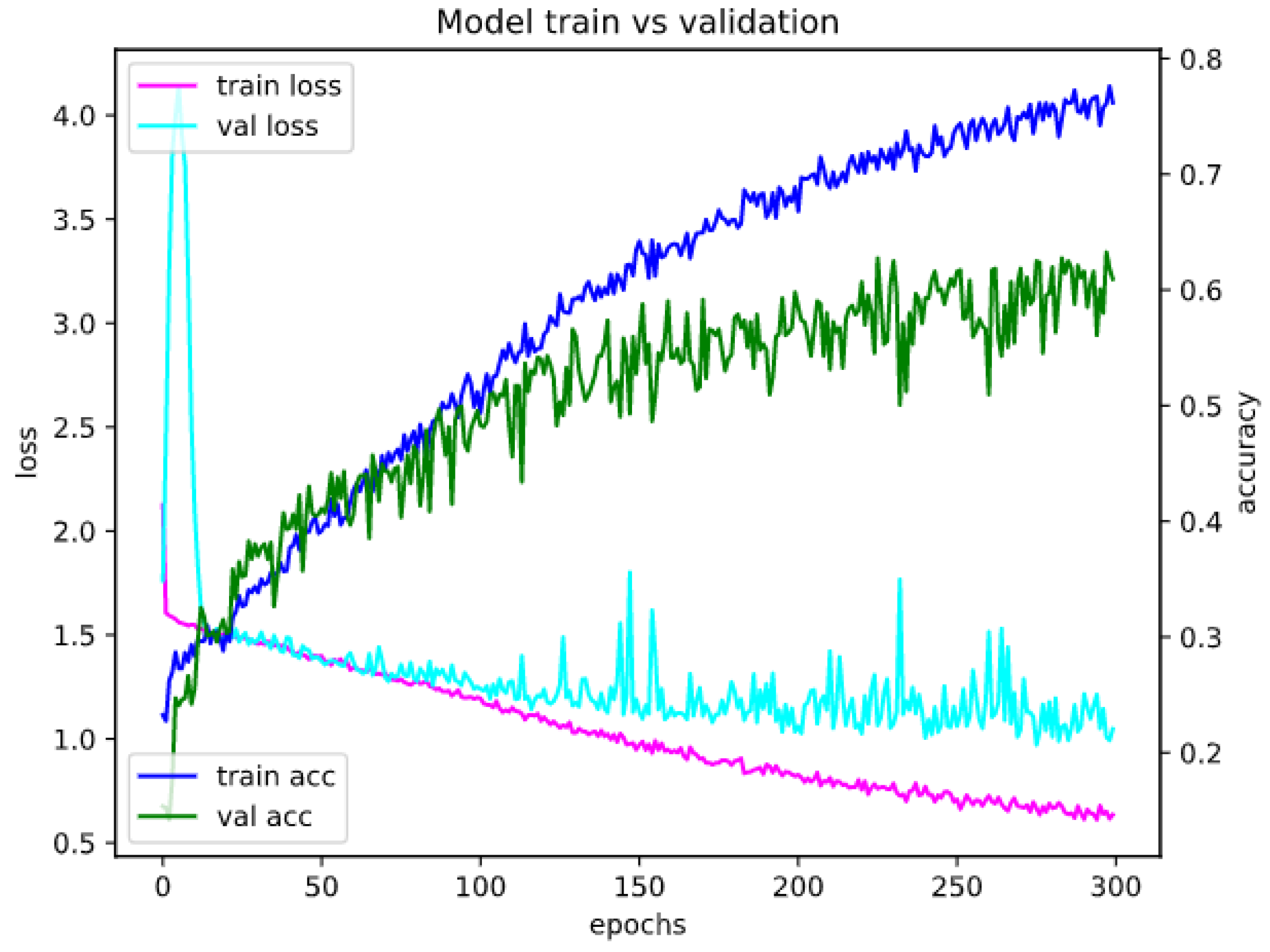
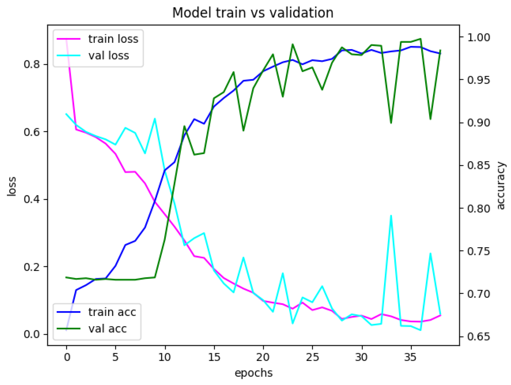
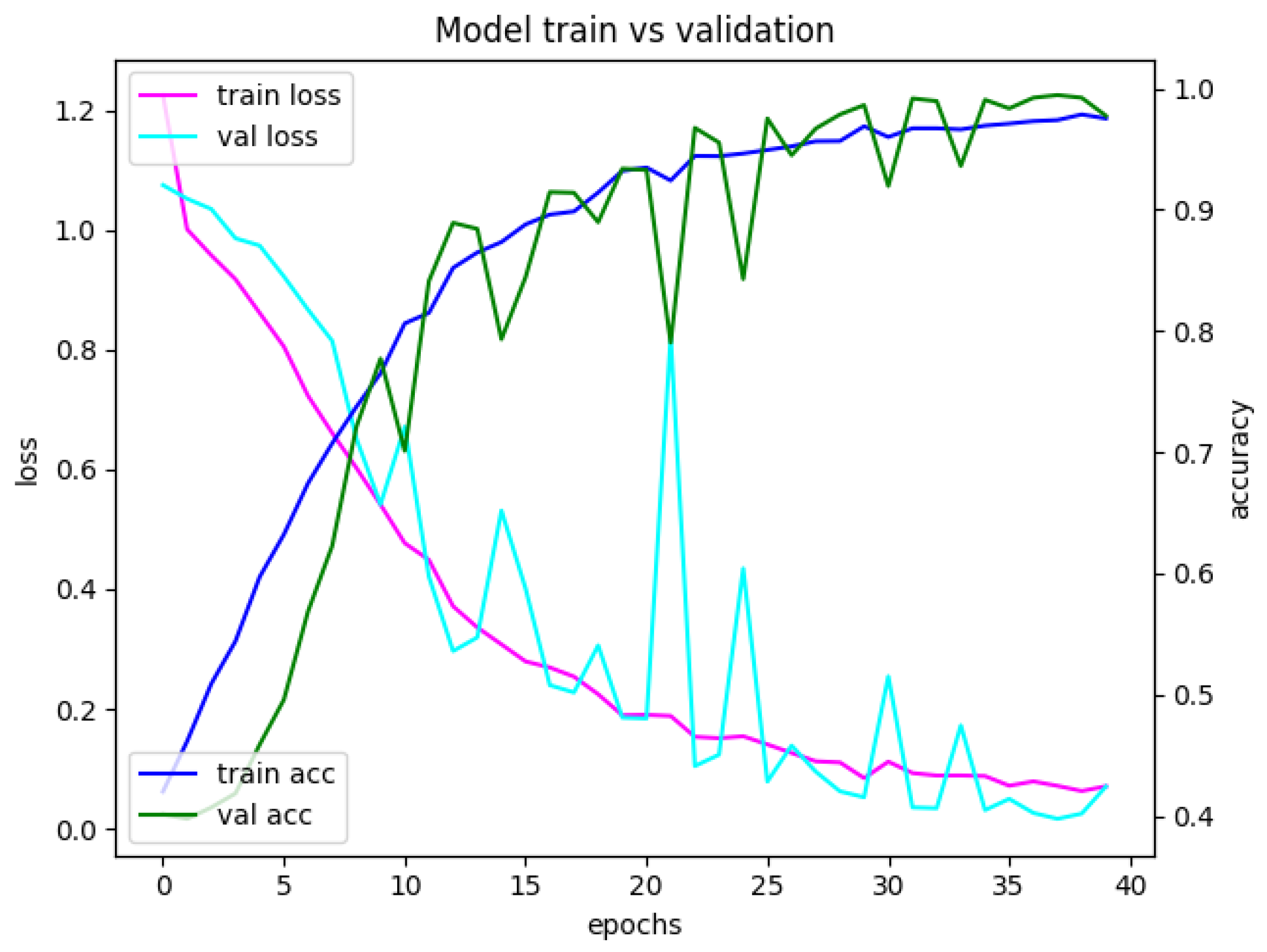
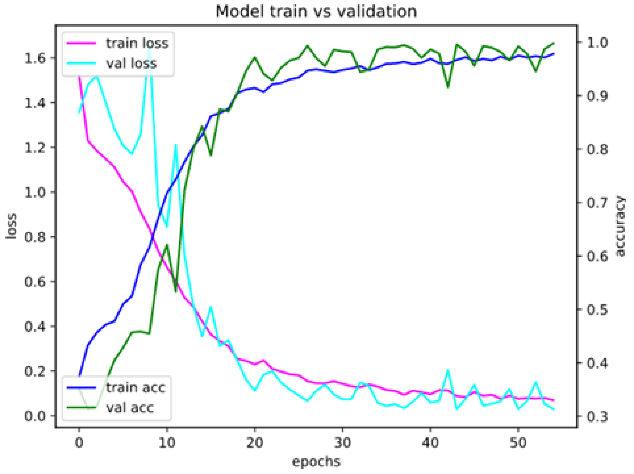
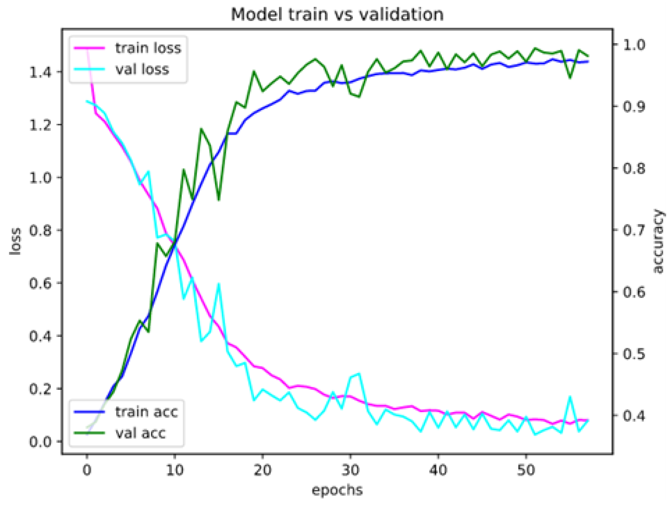
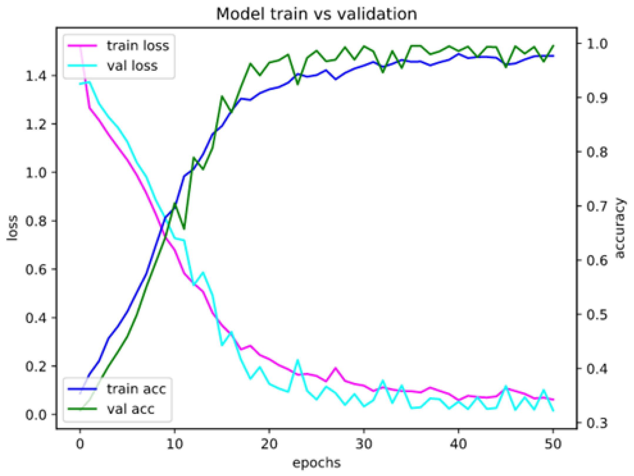
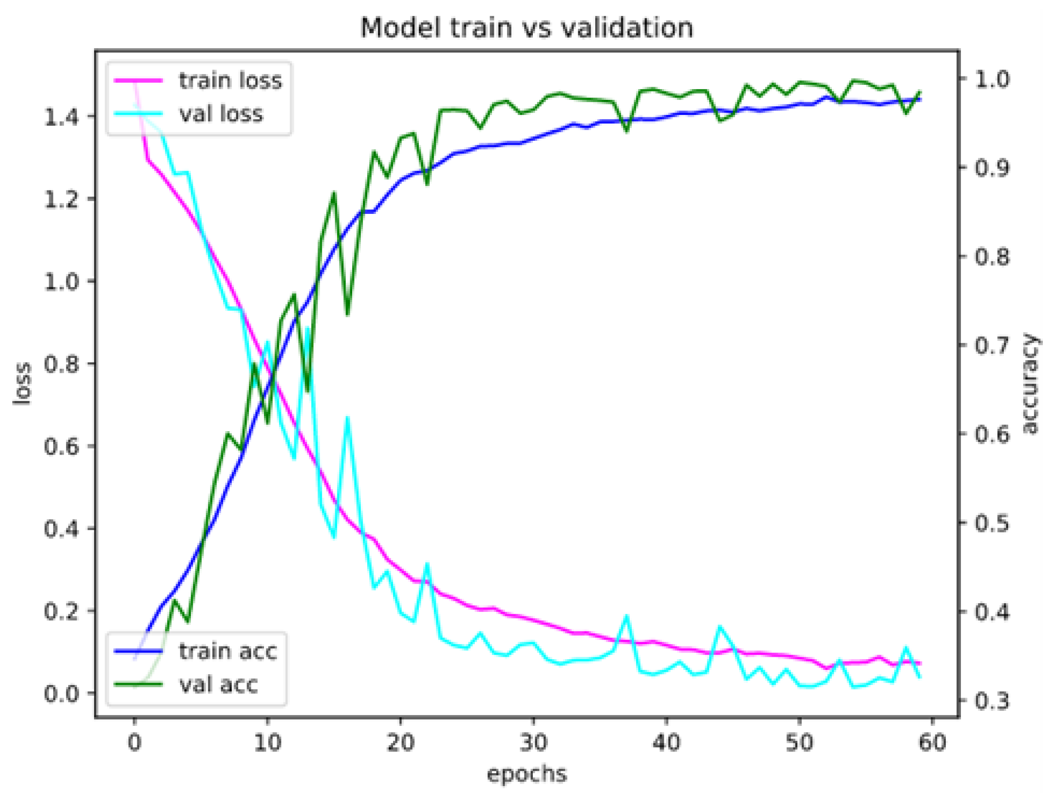
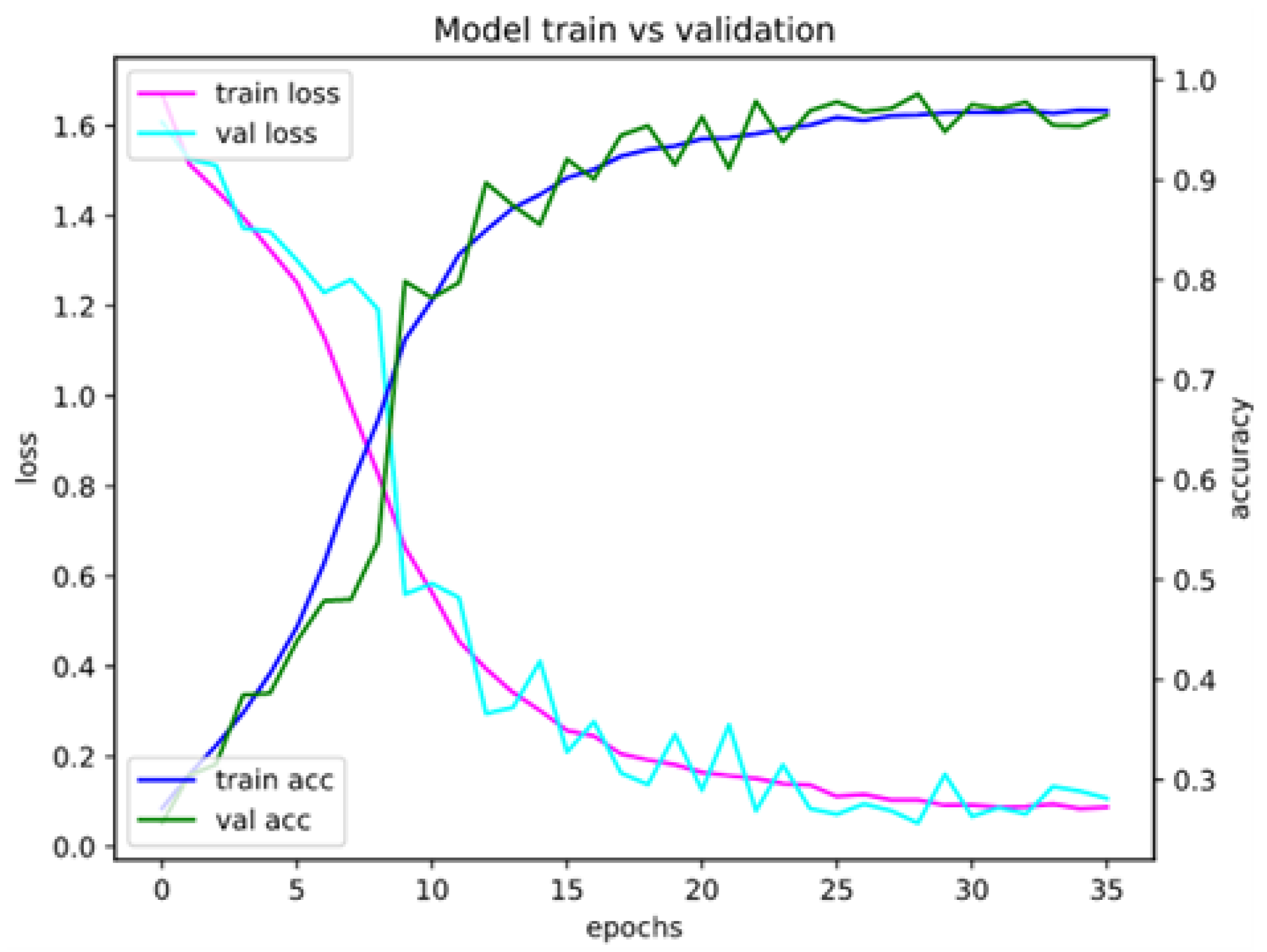
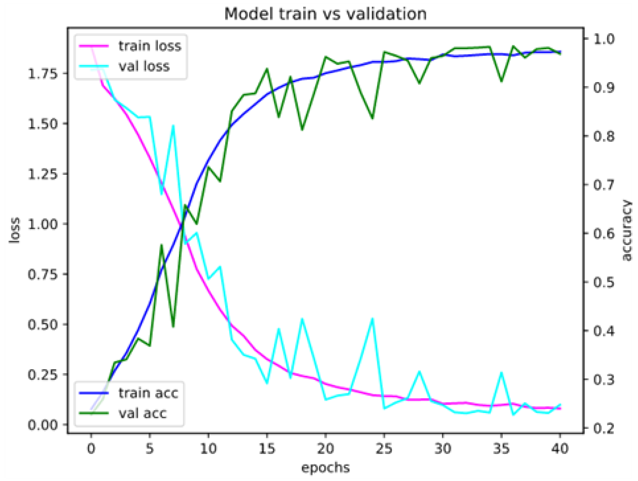
Appendix A. Model Assessment: Experimental Results in Details
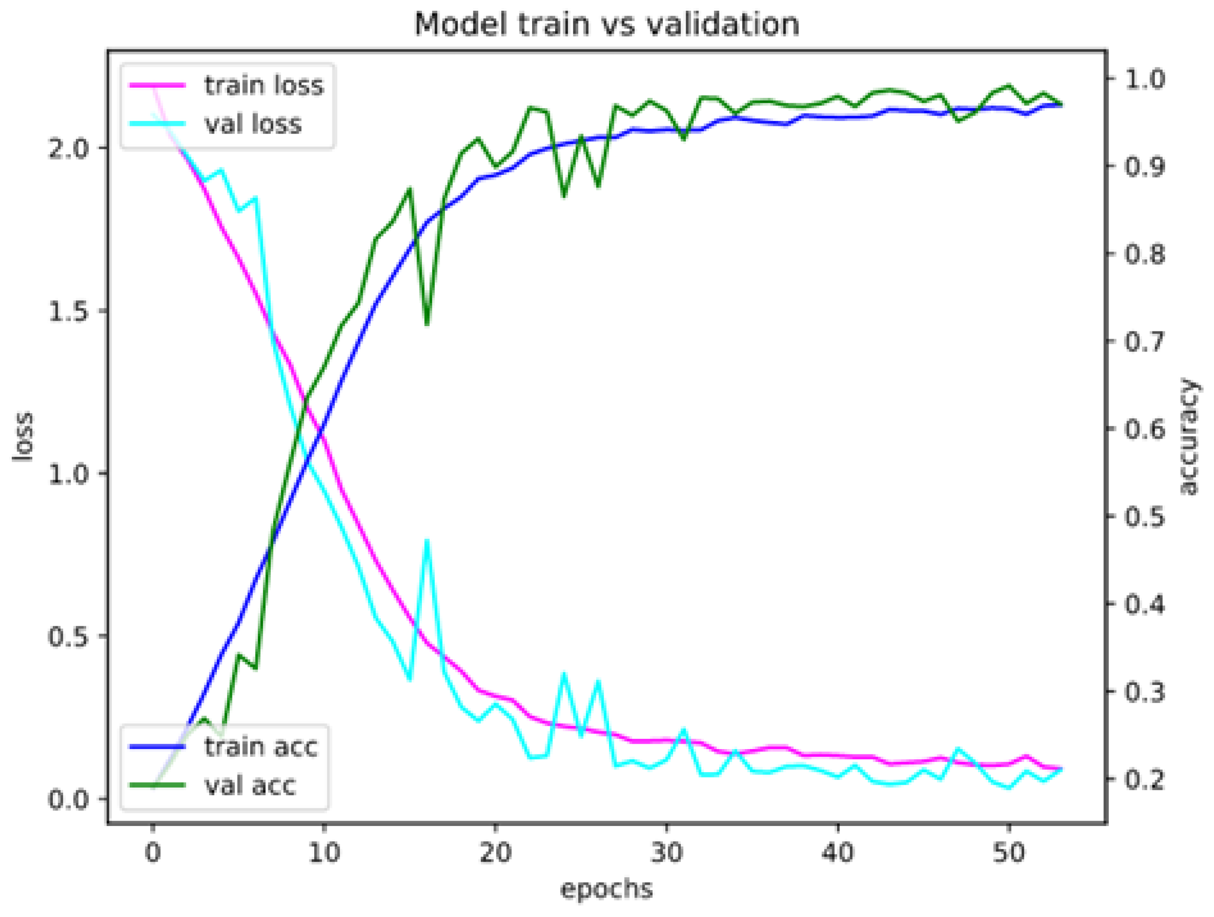
Appendix A.1. Accuracy and Loss for Different Sets of Recognized Accents


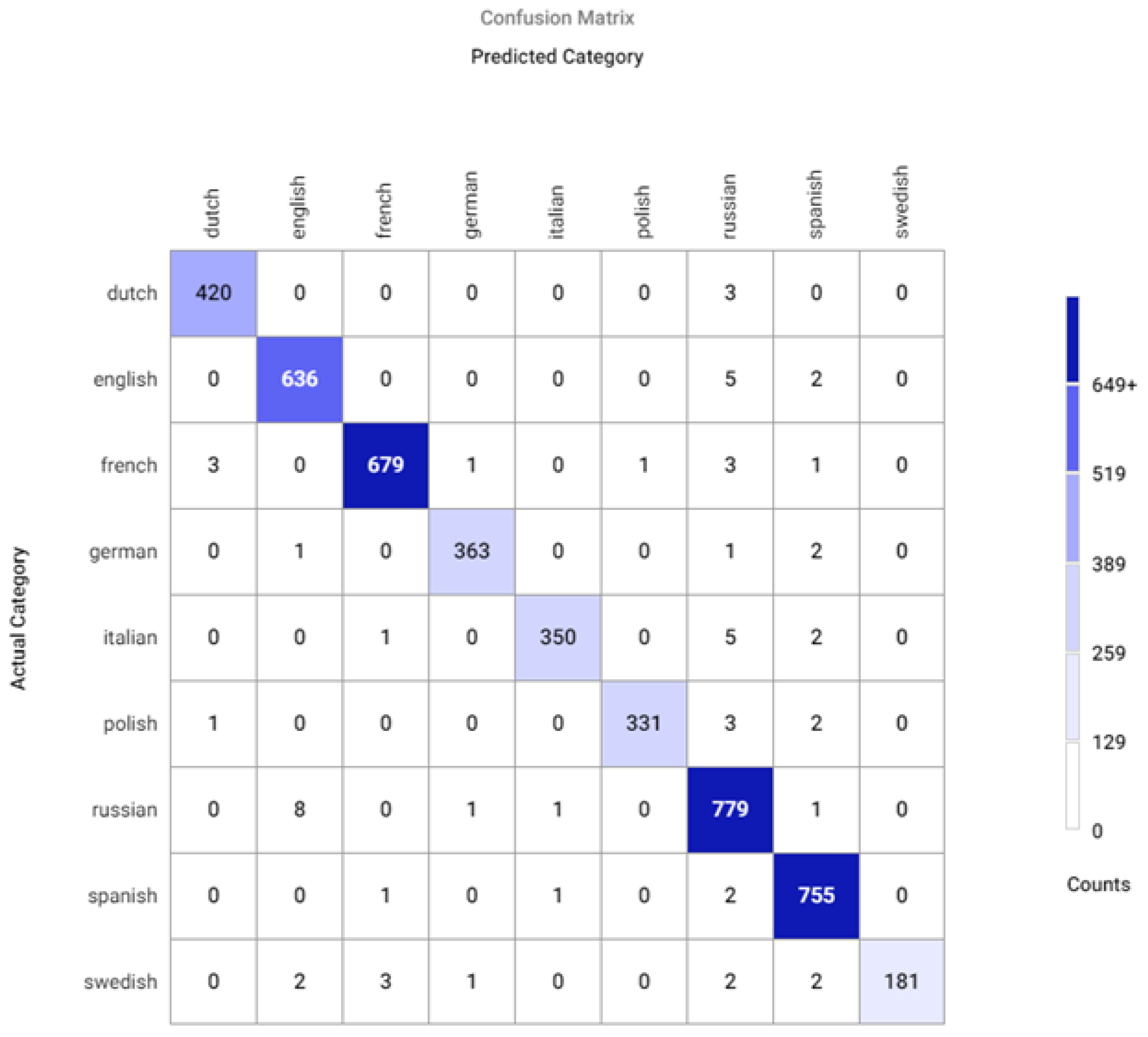
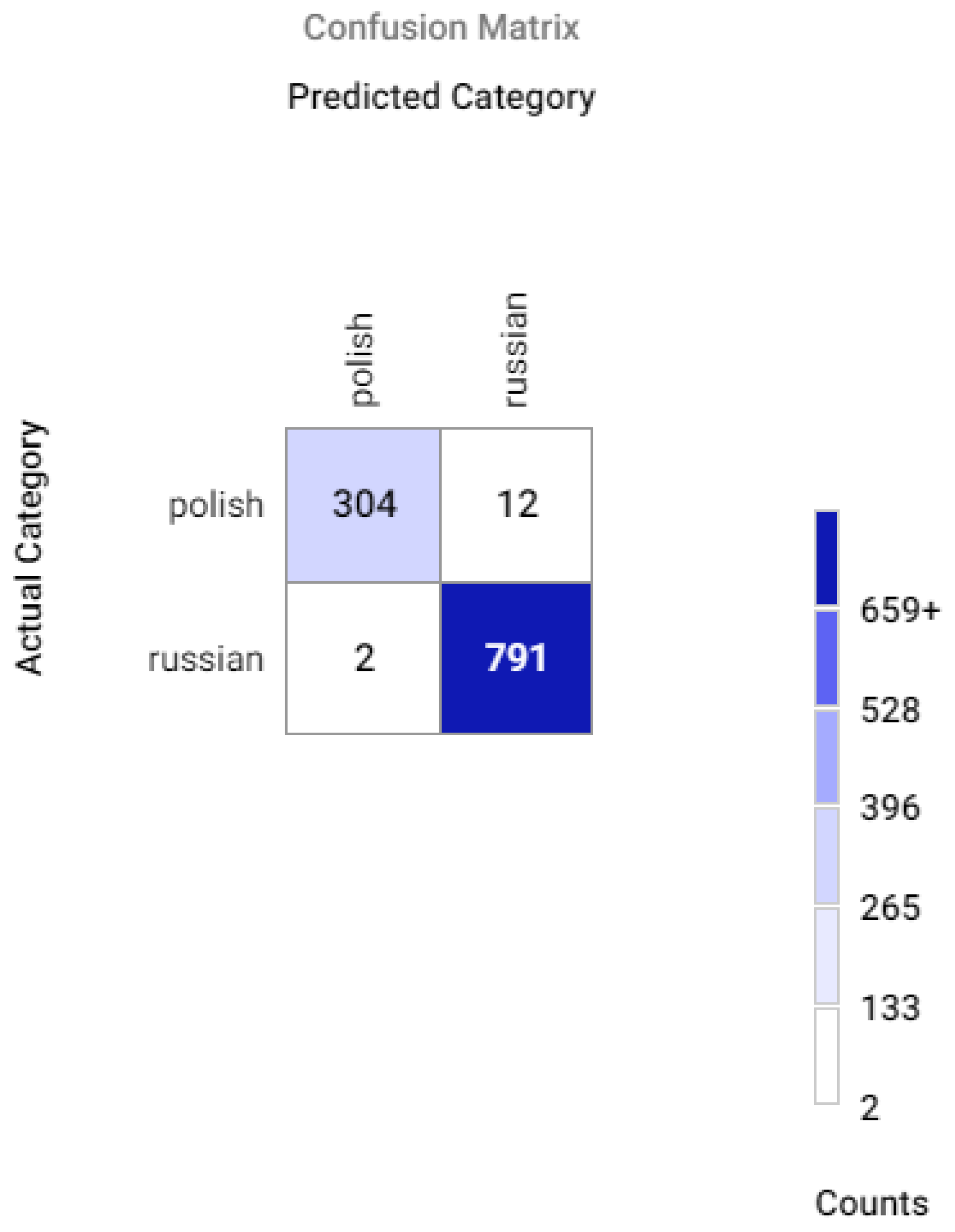
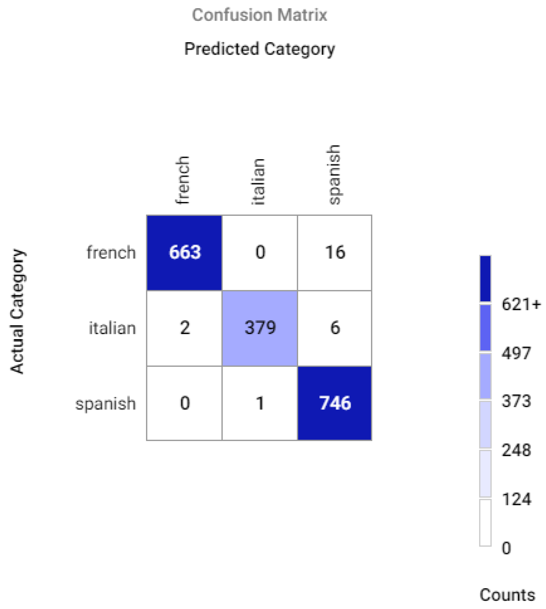
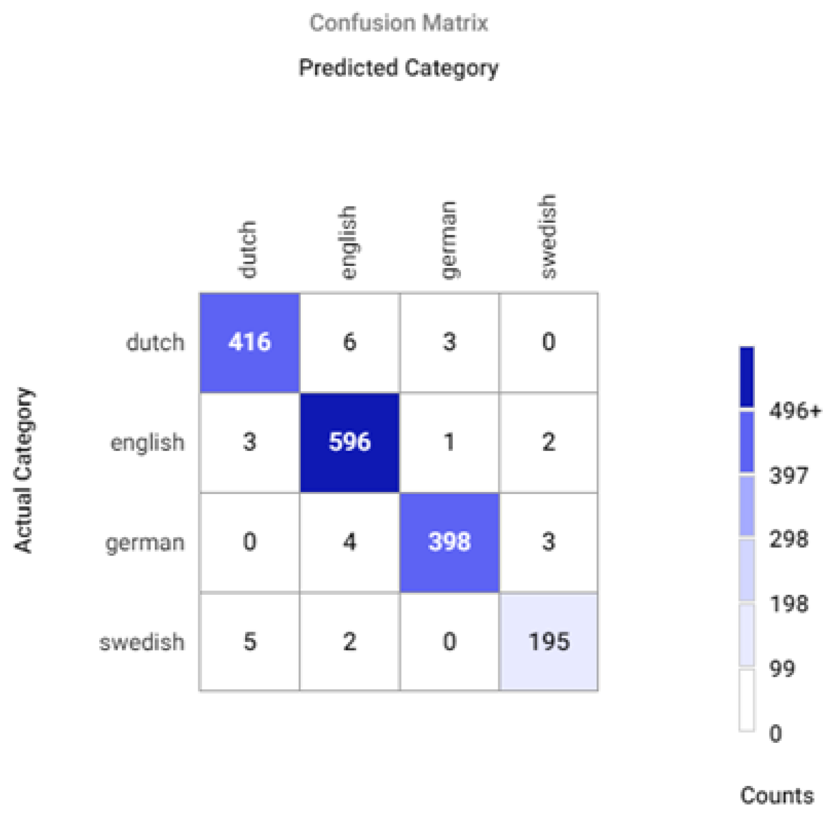
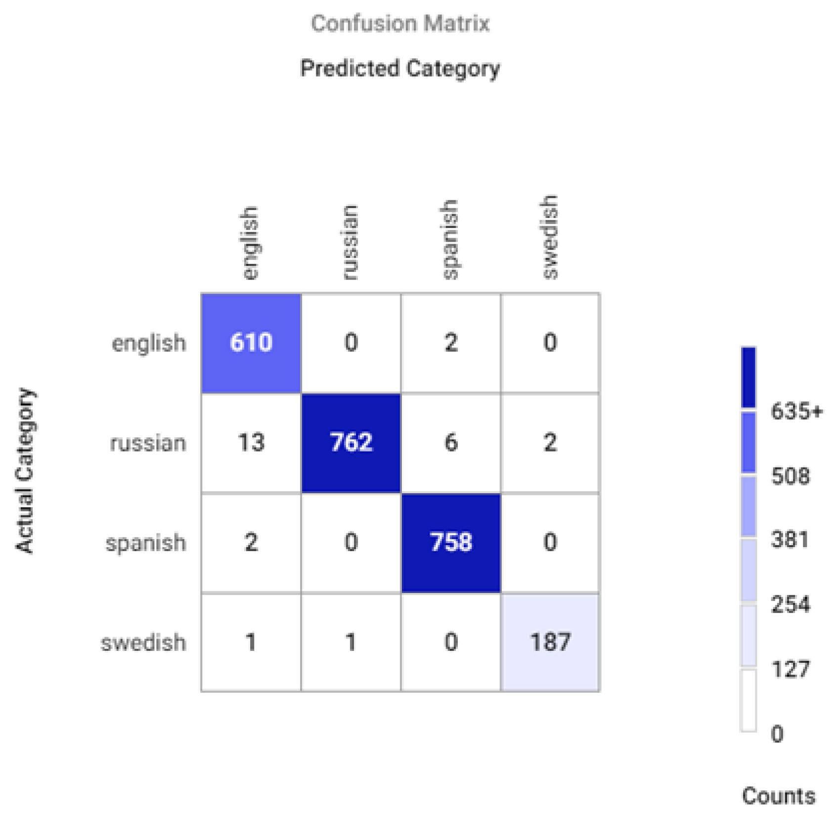
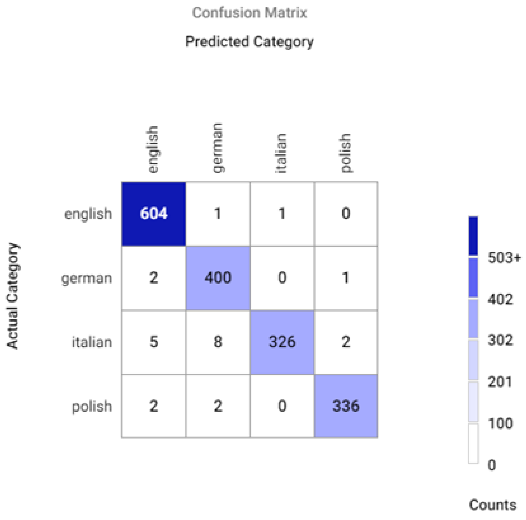
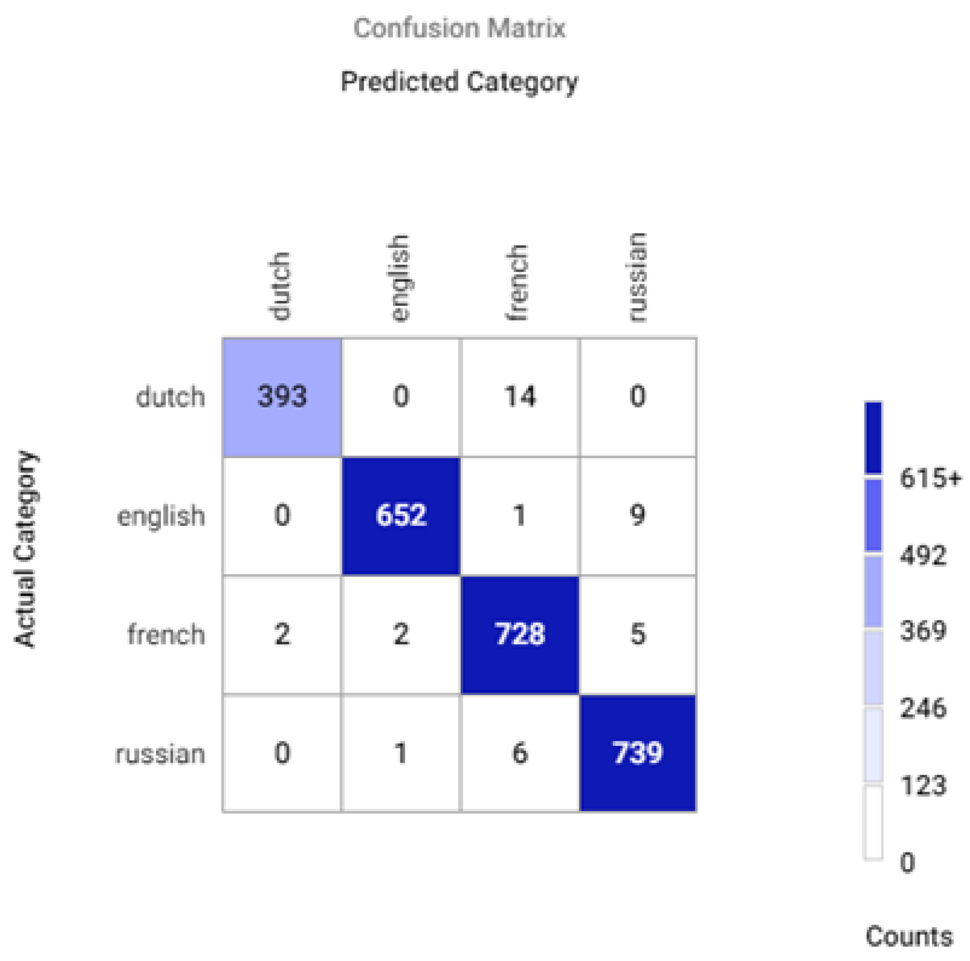
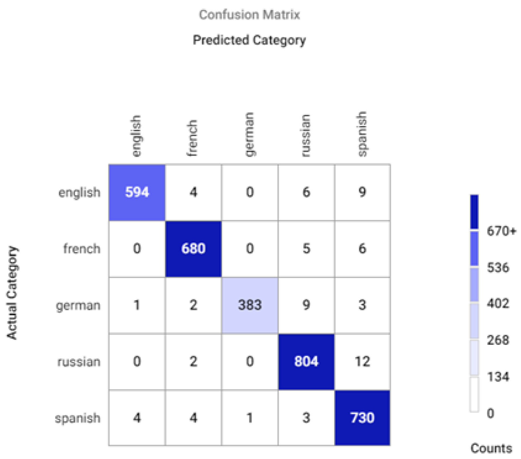
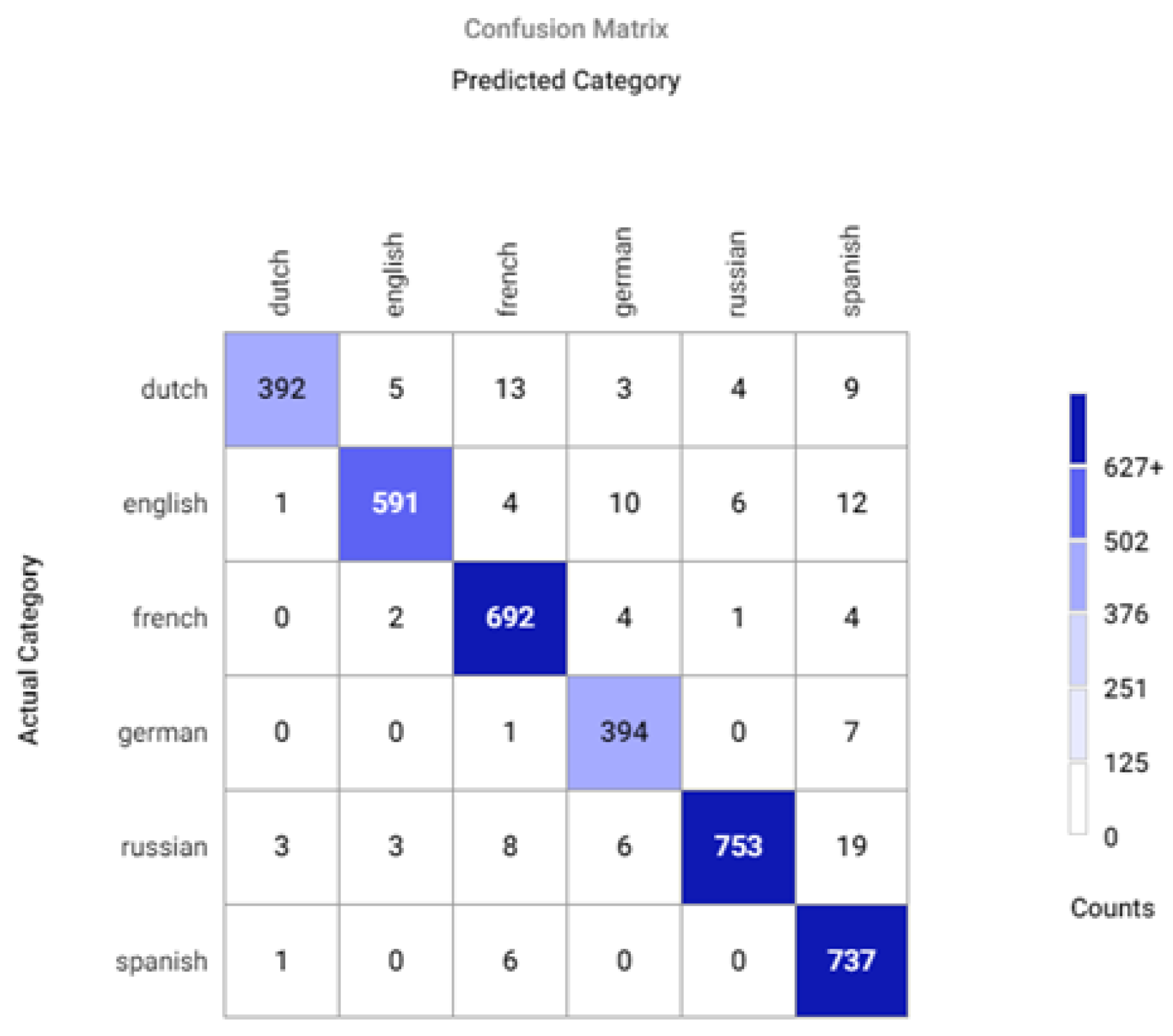
Appendix A.2. Confusion Matrices for Different Sets of Recognized Accents


References
- Boula de Mareüil, P.; Vieru, B. The Contribution of Prosody to the Perception of Foreign Accent. Phonetica 2006, 63, 247–267. [Google Scholar] [CrossRef] [PubMed]
- Rogerson-Revell, P.M. Computer-assisted pronunciation training (CAPT): Current issues and future directions. RELC J. 2021, 52, 189–205. [Google Scholar] [CrossRef]
- Jiang, S.W.F.; Yan, B.C.; Lo, T.H.; Chao, F.A.; Chen, B. Towards robust mispronunciation detection and diagnosis for L2 English learners with accent-modulating methods. In Proceedings of the 2021 IEEE Automatic Speech Recognition and Understanding Workshop (ASRU), Cartagena, Colombia, 13–17 December 2021; pp. 1065–1070. [Google Scholar]
- Algabri, M.; Mathkour, H.; Alsulaiman, M.; Bencherif, M.A. Mispronunciation Detection and Diagnosis with Articulatory-Level Feedback Generation for Non-Native Arabic Speech. Mathematics 2022, 10, 2727. [Google Scholar] [CrossRef]
- Singh, Y.; Pillay, A.; Jembere, E. Features of Speech Audio for Accent Recognition. In Proceedings of the 2020 International Conference on Artificial Intelligence, Big Data, Computing and Data Communication Systems (icABCD), Durban, South Africa, 6–7 August 2020; pp. 1–6. [Google Scholar] [CrossRef]
- Hansen, J.H.L.; Arslan, L.M. Foreign accent classification using source generator based prosodic features. In Proceedings of the 1995 International Conference on Acoustics, Speech, and Signal Processing, Detroit, MI, USA, 9–12 May 1995; Volume 1, pp. 836–839. [Google Scholar] [CrossRef]
- Huang, H.; Xiang, X.; Yang, Y.; Ma, R.; Qian, Y. Aispeech-sjtu accent identification system for the accented english speech recognition challenge. In Proceedings of the ICASSP 2021-2021 IEEE International Conference on Acoustics, Speech and Signal Processing (ICASSP), Toronto, ON, Canada, 6–11 June 2021; pp. 6254–6258. [Google Scholar]
- Deshpande, S.; Chikkerur, S.; Govindaraju, V. Accent classification in speech. In Proceedings of the Fourth IEEE Workshop on Automatic Identification Advanced Technologies (AutoID’05), Buffalo, NY, USA, 17–18 October 2005; pp. 139–143. [Google Scholar] [CrossRef]
- Huang, C.; Chen, T.; Chang, E. Accent Issues in Large Vocabulary Continuous Speech Recognition. Int. J. Speech Technol. 2004, 7, 141–153. [Google Scholar] [CrossRef]
- Tverdokhleb, E.; Dobrovolskyi, H.; Keberle, N.; Myronova, N. Implementation of accent recognition methods subsystem for eLearning systems. In Proceedings of the 2017 9th IEEE International Conference on Intelligent Data Acquisition and Advanced Computing Systems: Technology and Applications (IDAACS), Bucharest, Romania, 21–23 September 2017; Volume 2, pp. 1037–1041. [Google Scholar] [CrossRef]
- Ensslin, A.; Goorimoorthee, T.; Carleton, S.; Bulitko, V.; Poo Hernandez, S. Deep Learning for Speech Accent Detection in Video games. In Proceedings of the Thirteenth Artificial Intelligence and Interactive Digital Entertainment Conference, Salt Lake City, UT, USA, 5–9 October 2017; Volume 13. [Google Scholar]
- Berjon, P.; Nag, A.; Dev, S. Analysis of French phonetic idiosyncrasies for accent recognition. Soft Comput. Lett. 2021, 3, 100018. [Google Scholar] [CrossRef]
- Bird, J.; Wanner, E.; Ekárt, A.; Faria, D. Accent Classification in Human Speech Biometrics for Native and Non-native English Speakers. In Proceedings of the PErvasive Technologies Related to Assistive Environments (PETRA), Rhodes, Greece, 5–7 June 2019; pp. 554–560. [Google Scholar] [CrossRef]
- Zhang, Z.; Wang, Y.; Yang, J. Accent recognition with hybrid phonetic features. Sensors 2021, 21, 6258. [Google Scholar] [CrossRef]
- Malla, S.S. Acoustic Features Based Accent Classification of Kashmiri Language using Deep Learning. Glob. J. Comput. Sci. Technol. 2022, 22, 39–43. [Google Scholar]
- Graham, C. L1 Identification from L2 Speech Using Neural Spectrogram Analysis. Interspeech 2021, 2021, 3959–3963. [Google Scholar] [CrossRef]
- Ahamad, A.; Anand, A.; Bhargava, P. AccentDB: A Database of Non-Native English Accents to Assist Neural Speech Recognition. arXiv 2020, arXiv:2005.07973. [Google Scholar]
- Oladipo, F.; Habeeb, R.A.; Musa, A.E. Accent Identification of Ethnically Diverse Nigerian English Speakers. SSRN Electron. J. 2020. [Google Scholar] [CrossRef]
- Aswathi Sanal, M. Accent Recognition for Malayalam Speech Signals. Int. J. Innov. Res. Comput. Commun. Eng. 2017, 5, 4013–4017. [Google Scholar]
- Ma, Y.; Paulraj, M.; Yaacob, S.; Shahriman, A.; Nataraj, S.K. Speaker accent recognition through statistical descriptors of Mel-bands spectral energy and neural network model. In Proceedings of the 2012 IEEE Conference on Sustainable Utilization and Development in Engineering and Technology (STUDENT), Kuala Lumpur, Malaysia, 6–9 October 2012; pp. 262–267. [Google Scholar] [CrossRef]
- Duong, Q.T.; Do, V.H. Development of Accent Recognition Systems for Vietnamese Speech. In Proceedings of the 2021 24th Conference of the Oriental COCOSDA International Committee for the Co-ordination and Standardisation of Speech Databases and Assessment Techniques (O-COCOSDA), Singapore, 18–20 November 2021; pp. 174–179. [Google Scholar]
- Krishna, G.R.; Krishnan, R.; Mittal, V.K. A system for automatic regional accent classification. In Proceedings of the 2020 IEEE 17th India Council International Conference (INDICON), New Delhi, India, 10–13 December 2020; pp. 1–5. [Google Scholar]
- Cheng, J.; Bojja, N.; Chen, X. Automatic accent quantification of Indian speakers of English. In Proceedings of the Interspeech, Lyon, France, 25–29 August 2013; pp. 2574–2578. [Google Scholar]
- Lazaridis, A.; el Khoury, E.; Goldman, J.P.; Avanzi, M.; Marcel, S.; Garner, P.N. Swiss French Regional Accent Identification. In Proceedings of the Odyssey, Joensuu, Finland, 16–19 June 2014; pp. 106–111. [Google Scholar]
- Jiao, Y.; Tu, M.; Berisha, V.; Liss, J.M. Accent Identification by Combining Deep Neural Networks and Recurrent Neural Networks Trained on Long and Short Term Features. In Proceedings of the Interspeech, San Francisco, CA, USA, 8–12 September 2016; pp. 2388–2392. [Google Scholar]
- Weninger, F.; Sun, Y.; Park, J.; Willett, D.; Zhan, P. Deep Learning Based Mandarin Accent Identification for Accent Robust ASR. In Proceedings of the Interspeech, Graz, Austria, 15–19 September 2019; pp. 510–514. [Google Scholar]
- Işik, G.; Artuner, H. Turkish Dialect Recognition Using Acoustic and Phonotactic Features in Deep Learning Architectures. J. Inf. Technol. 2020, 13, 207–216. [Google Scholar]
- Kethireddy, R.; Kadiri, S.R.; Alku, P.; Gangashetty, S.V. Mel-Weighted Single Frequency Filtering Spectrogram for Dialect Identification. IEEE Access 2020, 8, 174871–174879. [Google Scholar] [CrossRef]
- George Mason University. Speech Accent Archive. 2021. Available online: https://accent.gmu.edu/ (accessed on 8 August 2022).
- Zheng, F.; Zhang, G.; Song, Z. Comparison of different implementations of MFCC. J. Comput. Sci. Technol. 2001, 16, 582–589. [Google Scholar] [CrossRef]
- Liu, S.; Wang, D.; Cao, Y.; Sun, L.; Wu, X.; Kang, S.; Wu, Z.; Liu, X.; Su, D.; Yu, D.; et al. End-to-end accent conversion without using native utterances. In Proceedings of the ICASSP 2020—2020 IEEE International Conference on Acoustics, Speech and Signal Processing (ICASSP), Barcelona, Spain, 4–8 May 2020; pp. 6289–6293. [Google Scholar]
- Rasier, L.; Hiligsmann, P. Prosodic transfer from L1 to L2. Theoretical and methodological issues. Nouv. Cah. Linguist. Française 2007, 28, 41–66. [Google Scholar]
- Alain de Cheveigné, H.K. YIN, a fundamental frequency estimator for speech and music. J. Acoust. Soc. Am. 2002, 111, 1917–1930. [Google Scholar] [CrossRef] [PubMed]
- Shimodaira, H. Improving predictive inference under covariate shift by weighting the log-likelihood function. J. Stat. Plan. Inference 2000, 90, 227–244. [Google Scholar] [CrossRef]
- Ioffe, S.; Szegedy, C. Batch Normalization: Accelerating Deep Network Training by Reducing Internal Covariate Shift. In Proceedings of the 32nd International Conference on Machine Learning, Lille, France, 6–11 July 2015; Bach, F., Blei, D., Eds.; PMLR: Lille, France, 2015; Volume 37, pp. 448–456. [Google Scholar]
- Moreno-Torres, J.G.; Raeder, T.; Alaiz-Rodríguez, R.; Chawla, N.V.; Herrera, F. A unifying view on dataset shift in classification. Pattern Recognit. 2012, 45, 521–530. [Google Scholar] [CrossRef]
- Nair, N.G.; Satpathy, P.; Christopher, J. Covariate Shift: A Review and Analysis on Classifiers. In Proceedings of the 2019 Global Conference for Advancement in Technology (GCAT), Bangalore, India, 18–20 October 2019; pp. 1–6. [Google Scholar] [CrossRef]
- Bock, S.; Weiß, M. A proof of local convergence for the Adam optimizer. In Proceedings of the 2019 International Joint Conference on Neural Networks (IJCNN), Budapest, Hungary, 14–19 July 2019; pp. 1–8. [Google Scholar]
- Longford, N.T. A fast scoring algorithm for maximum likelihood estimation in unbalanced mixed models with nested random effects. Biometrika 1987, 74, 817–827. [Google Scholar] [CrossRef]
- Wu, T.; Duchateau, J.; Martens, J.P.; Van Compernolle, D. Feature subset selection for improved native accent identification. Speech Commun. 2010, 52, 83–98. [Google Scholar] [CrossRef]
- Sun, L.; Wang, T.; Ding, W.; Xu, J.; Lin, Y. Feature selection using Fisher score and multilabel neighborhood rough sets for multilabel classification. Inf. Sci. 2021, 578, 887–912. [Google Scholar] [CrossRef]
- Milner, B.; Shao, X. Prediction of Fundamental Frequency and Voicing From Mel-Frequency Cepstral Coefficients for Unconstrained Speech Reconstruction. IEEE Trans. Audio Speech Lang. Process. 2007, 15, 24–33. [Google Scholar] [CrossRef]
- Bogach, N.; Boitsova, E.; Chernonog, S.; Lamtev, A.; Lesnichaya, M.; Lezhenin, I.; Novopashenny, A.; Svechnikov, R.; Tsikach, D.; Vasiliev, K.; et al. Speech Processing for Language Learning: A Practical Approach to Computer-Assisted Pronunciation Teaching. Electronics 2021, 10, 235. [Google Scholar] [CrossRef]
- Mikhailava, V.; Blake, J.; Pyshkin, E.; Bogach, N.; Chernonog, S.; Zhuikov, A.; Lesnichaya, M.; Lezhenin, I.; Svechnikov, R. Dynamic Assessment during Suprasegmental Training with Mobile CAPT. Proc. Speech Prosody 2022, 2022, 430–434. [Google Scholar]
- Feng, Y.; Fu, G.; Chen, Q.; Chen, K. SED-MDD: Towards sentence dependent end-to-end mispronunciation detection and diagnosis. In Proceedings of the ICASSP 2020-2020 IEEE International Conference on Acoustics, Speech and Signal Processing (ICASSP), Barcelona, Spain, 4–8 May 2020; pp. 3492–3496. [Google Scholar]


| Paper, Year | Feature Set | Model | Classes | Accents | Dataset |
|---|---|---|---|---|---|
| [15], 2022 | Mel-spectrogram | CNN | 5 | 5 Kashmiri accents | Custom |
| [16], 2021 | SG | CNN (LeNet) | 5 | DU, FR, JA, NS, PO | IViE, Cambridge English Corpus |
| [12], 2021 | SG | CNN | 5 | AR, FR, GE, IN, NS | SAA |
| [5], 2020 | MFCC, SG, CG, SC, SR | CNN | 5 | AR, FR, NS, SP, ZH | SAA |
| 3 | AR, NS, ZH | ||||
| [17], 2020 | MFCC | CNN with attention | 2 | IN, NS | Custom |
| 4 | IN | ||||
| 9 | IN, NS | ||||
| [18], 2020 | MFCC | Logistic Regression | 3 | HA, IG, YO | Custom |
| [13], 2019 | MFCC | LSTM, RF | 4 | NS, SP | Custom |
| [10], 2017 | MFCC, LPCC | FFNN | 6 | GA, IN, IT, JA, KO, NS | Wildcat |
| [11], 2017 | SG | CNN (AlexNet) | 3 | NS, SP | SAA |
| [19], 2017 | MFCC | GMM | 3 | ML | Custom |
| [20], 2012 | Mel-spectrogram statistics | FF-MLP | 3 | IN, MS, ZH | Custom |
| [8], 2005 | 2nd and 3rd formants | GMM | 2 | IN, NS | Custom (SAA subset) |
| Fragments of Silence | ||||
|---|---|---|---|---|
| L1 | Preserved | Removed | ||
| Accuracy | Error | Accuracy | Error | |
| EN RU SP SW | 0.71 | 0.83 | 0.70 | 0.84 |
| FR IT SP | 0.71 | 0.73 | 0.68 | 0.82 |
| L1 | Most Effective Settings | Error Compared to Kernel Size = (3, 3) and Pool Size = (2, 2) | ||
|---|---|---|---|---|
| Kernel Size | Pool Size | MFCC | 30 Attribute | |
| PO RU | (3, 3) | (3, 3) | −6% | −4% |
| FR IT SP | (5, 5) | (3, 3) | −8% | −11% |
| DU EN GE SW | (3, 3) | (3, 3) | +3% | −13% |
| EN RU SP SW | (3, 3) | (3, 3) | −11% | −16% |
| EN GE IT PO | (3, 3) | (3, 3) | −4% | −9% |
| DU EN FR RU | (5, 5) | (3, 3) | −5% | - |
| French, Italian, Spanish (Romance Languages) | ||||
|---|---|---|---|---|
| Kernel Size | Pool Size | Learning Time (mm:ss) | Accuracy | Error |
| (3, 3) | (2, 2) | 41:06 | 0.9889 | 0.0614 |
| (3, 3) | (3, 3) | 20:01 | 0.9904 | 0.0261 |
| (5, 5) | (3, 3) | 17:57 | 0.9852 | 0.0564 |
| (7, 7) | (3, 3) | 26:14 | 0.9867 | 0.0468 |
| English, Spanish, Swedish, Russian (Mixed Group) | ||||
|---|---|---|---|---|
| Maximum Horizontal Shift during Augmentation | ||||
| Features | 0.05 | 0.1 | ||
| Accuracy | Error | Accuracy | Error | |
| MFCC | 0.65 | 0.94 | 0.65 | 0.86 |
| MFCC + | 0.68 | 0.84 | 0.72 | 0.78 |
| MFCC + spectral centroid | 0.65 | 0.93 | 0.66 | 0.86 |
| French, Italian, Spanish (Romance Languages) | ||
|---|---|---|
| Horizontal Shift | Accuracy | Error |
| 0.05 | 0.75 | 0.62 |
| 0.1 | 0.75 | 0.59 |
| 0.15 | 0.74 | 0.62 |
| 0.2 | 0.77 | 0.55 |
| 0.25 | 0.75 | 0.58 |
| 0.3 | 0.76 | 0.58 |
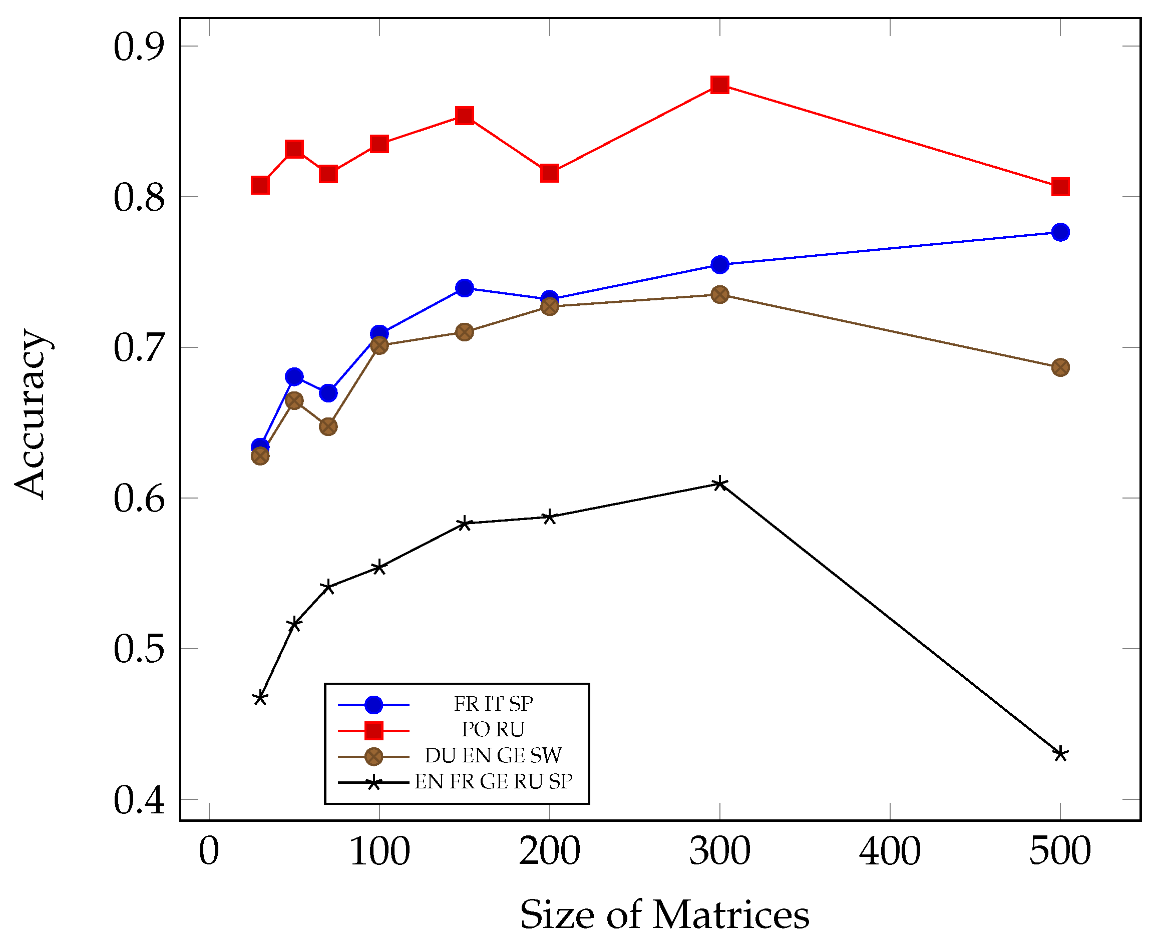
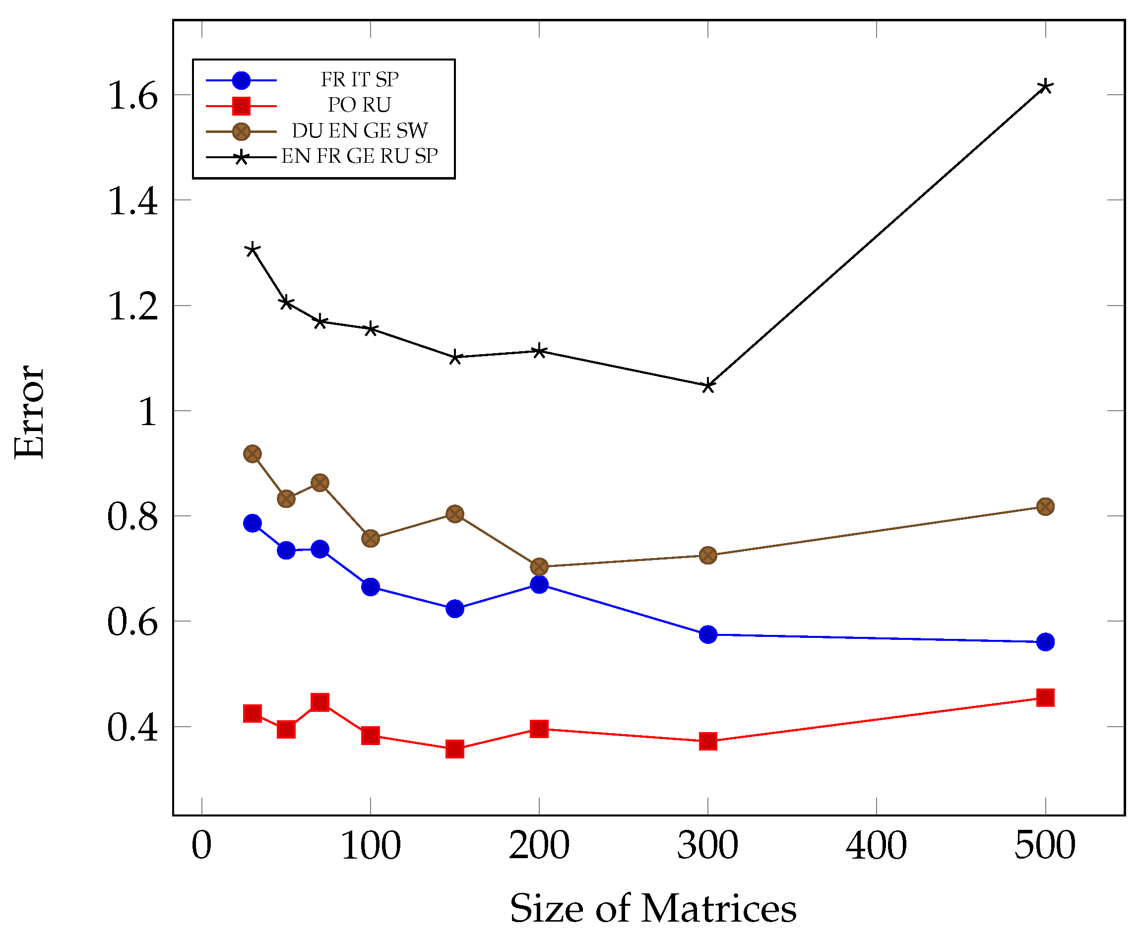
| Size of Feature Matrices | Accuracy | Error |
|---|---|---|
| Russian, Polish (Slavic Languages) | ||
| 30 | 0.8075 | 0.4248 |
| 50 | 0.8315 | 0.3946 |
| 70 | 0.8151 | 0.4458 |
| 100 | 0.835 | 0.3828 |
| 150 | 0.8537 | 0.3573 |
| 200 | 0.8156 | 0.3956 |
| 300 | 0.8742 | 0.372 |
| 500 | 0.8065 | 0.4547 |
| French, Italian, Spanish (Romance Languages) | ||
| 30 | 0.6337 | 0.7862 |
| 50 | 0.6804 | 0.7346 |
| 70 | 0.6696 | 0.7371 |
| 100 | 0.7088 | 0.6652 |
| 150 | 0.7393 | 0.6238 |
| 200 | 0.7318 | 0.6699 |
| 300 | 0.7548 | 0.5748 |
| 500 | 0.7764 | 0.5607 |
| Size of Feature Matrices | Accuracy | Error |
|---|---|---|
| English, German, Dutch, Swedish (Anglo-Saxon group) | ||
| 30 | 0.6278 | 0.918 |
| 50 | 0.6646 | 0.8325 |
| 70 | 0.6473 | 0.8631 |
| 100 | 0.7012 | 0.7572 |
| 150 | 0.7101 | 0.8038 |
| 200 | 0.727 | 0.7033 |
| 300 | 0.735 | 0.7251 |
| 500 | 0.6866 | 0.8178 |
| English, Spanish, German, Russian, French (Mixed group) | ||
| 30 | 0.4674 | 1.3059 |
| 50 | 0.5162 | 1.2053 |
| 70 | 0.5409 | 1.1692 |
| 100 | 0.554 | 1.1555 |
| 150 | 0.583 | 1.1013 |
| 200 | 0.5874 | 1.1133 |
| 300 | 0.6095 | 1.0474 |
| 500 | 0.4302 | 1.6158 |
| French, Italian, Spanish (Romance Languages) | ||||
|---|---|---|---|---|
| Number of Mel-Bands | Size of Input Matrices | Training Time (hh:mm:ss) | Accuracy | Error |
| 32 | 30 | 00:11:06 | 0.8889 | 0.2837 |
| 50 | 00:13:10 | 0.9239 | 0.2004 | |
| 75 | 00:13:20 | 0.9586 | 0.1216 | |
| 100 | 00:14:53 | 0.9483 | 0.1539 | |
| 150 | 00:12:16 | 0.9207 | 0.2347 | |
| 200 | 00:15:03 | 0.8675 | 0.3186 | |
| 64 | 30 | 00:28:55 | 0.9737 | 0.0858 |
| 50 | 00:19:48 | 0.9987 | 0.0406 | |
| 75 | 00:19:16 | 0.9912 | 0.033 | |
| 100 | 00:17:57 | 0.9852 | 0.0564 | |
| 150 | 00:25:15 | 0.9877 | 0.0398 | |
| 200 | 00:36:25 | 0.9593 | 0.1443 | |
| 128 | 100 | 01:23:56 | 0.9985 | 0.0074 |
| 150 | 01:31:14 | 0.9832 | 0.0873 | |
| Features | Test Accuracy | Test Error |
|---|---|---|
| Russian, Polish (Slavic Languages) | ||
| Threshold Accuracy—0.72 | ||
| MFCC | 0.84 | 0.37 |
| MFCC + | 0.83 | 0.4 |
| MFCC + spectral centroid | 0.85 | 0.39 |
| MFCC + spectral decay | 0.84 | 0.4 |
| MFCC + chromogram | 0.79 | 0.44 |
| MFCC + ZCR | 0.84 | 0.38 |
| MFCC + RMS | 0.83 | 0.41 |
| All | 0.81 | 0.41 |
| French, Italian, Spanish (Romance Languages) | ||
| Threshold Accuracy—0.43 | ||
| MFCC | 0.75 | 0.6 |
| MFCC + | 0.69 | 0.71 |
| MFCC + spectral centroid | 0.67 | 0.73 |
| MFCC + spectral decay | 0.68 | 0.72 |
| MFCC + chromogram | 0.63 | 0.84 |
| MFCC + ZCR | 0.71 | 0.68 |
| MFCC + RMS | 0.7 | 0.7 |
| All | 0.66 | 0.8 |
| Features | Test Accuracy | Test Error |
|---|---|---|
| English, Italian, German, Polish (Mixed group) | ||
| Threshold Accuracy—0.29 | ||
| MFCC | 0.62 | 1.00 |
| MFCC + | 0.65 | 0.88 |
| MFCC + spectral centroid | 0.61 | 0.94 |
| MFCC + spectral decay | 0.63 | 0.96 |
| MFCC + chromogram | Threshold not passed | |
| MFCC + ZCR | 0.64 | 0.9 |
| MFCC + RMS | 0.64 | 0.91 |
| All | 0.6 | 0.95 |
| English, Spanish, Swedish, Russian (Mixed group) | ||
| Threshold Accuracy—0.33 | ||
| MFCC | 0.72 | 0.81 |
| MFCC + | 0.71 | 0.83 |
| MFCC + spectral centroid | 0.68 | 0.88 |
| MFCC + spectral decay | 0.68 | 0.93 |
| MFCC + chromogram | 0.68 | 0.92 |
| MFCC + ZCR | 0.68 | 0.85 |
| MFCC + RMS | 0.67 | 0.95 |
| All | 0.75 | 0.7 |
| Accents | Accuracy | Loss |
|---|---|---|
| PO RU | 0.987 | 0.039 |
| FR IT SP | 0.986 | 0.052 |
| DU EN GE SW | 0.982 | 0.075 |
| EN RU SP SW | 0.988 | 0.042 |
| EN GE IT PO | 0.985 | 0.053 |
| DU EN FR RU | 0.984 | 0.039 |
| EN FR GE RU SP | 0.978 | 0.071 |
| DU EN FR GE RU SP | 0.964 | 0.097 |
| DU EN FR GE IT PO RU SP SW | 0.986 | 0.044 |
| Average | 0.982 | 0.056 |
| Source | Classifier | Number of Classes Recognized | Precision | Accuracy of CNNs Trained on Mel-Amplitude Spectrograms on a Linear Scale |
|---|---|---|---|---|
| [17] | CNN (with attention mechanism) | 2 | 1.0 | 0.987 |
| 4 | 0.99 | 0.984 | ||
| 9 | 0.995 | 0.986 | ||
| [11] | CNN (AlexNet) | 3 | 0.61 | 0.986 |
| [8] | GMM | 2 | 0.862 | 0.987 |
| [10] | FFNN | 6 | 0.914 | 0.964 |
| [5] | CNN | 3 | 0.703 | 0.986 |
| 5 | 0.539 | 0.978 | ||
| [20] | FF-MLP | 3 | 0.99 | 0.986 |
| Class | Precision | Recall | F1 |
|---|---|---|---|
| DU | 0.985 | 0.965 | 0.975 |
| EN | 0.984 | 0.983 | 0.983 |
| FR | 0.98 | 0.984 | 0.982 |
| GE | 0.978 | 0.98 | 0.98 |
| IT | 0.997 | 0.973 | 0.987 |
| PO | 0.993 | 0.977 | 0.987 |
| RU | 0.983 | 0.98 | 0.983 |
| SP | 0.968 | 0.992 | 0.978 |
| SW | 0.987 | 0.97 | 0.977 |
| Average | 0.984 | 0.978 | 0.981 |
Publisher’s Note: MDPI stays neutral with regard to jurisdictional claims in published maps and institutional affiliations. |
© 2022 by the authors. Licensee MDPI, Basel, Switzerland. This article is an open access article distributed under the terms and conditions of the Creative Commons Attribution (CC BY) license (https://creativecommons.org/licenses/by/4.0/).
Share and Cite
Mikhailava, V.; Lesnichaia, M.; Bogach, N.; Lezhenin, I.; Blake, J.; Pyshkin, E. Language Accent Detection with CNN Using Sparse Data from a Crowd-Sourced Speech Archive. Mathematics 2022, 10, 2913. https://0-doi-org.brum.beds.ac.uk/10.3390/math10162913
Mikhailava V, Lesnichaia M, Bogach N, Lezhenin I, Blake J, Pyshkin E. Language Accent Detection with CNN Using Sparse Data from a Crowd-Sourced Speech Archive. Mathematics. 2022; 10(16):2913. https://0-doi-org.brum.beds.ac.uk/10.3390/math10162913
Chicago/Turabian StyleMikhailava, Veranika, Mariia Lesnichaia, Natalia Bogach, Iurii Lezhenin, John Blake, and Evgeny Pyshkin. 2022. "Language Accent Detection with CNN Using Sparse Data from a Crowd-Sourced Speech Archive" Mathematics 10, no. 16: 2913. https://0-doi-org.brum.beds.ac.uk/10.3390/math10162913