

Deep Learning-Based Plant-Image Classification Using a Small Training Dataset

Division of Electronics and Electrical Engineering, Dongguk University, 30 Pildong-ro, 1-gil, Jung-gu, Seoul 04620, Korea
*
Author to whom correspondence should be addressed.
Mathematics 2022, 10(17), 3091; https://0-doi-org.brum.beds.ac.uk/10.3390/math10173091
Submission received: 6 July 2022
/
Revised: 10 August 2022
/
Accepted: 23 August 2022
/
Published: 28 August 2022
(This article belongs to the Special Issue Computational Intelligent and Image Processing)
Abstract
:Extensive research has been conducted on image augmentation, segmentation, detection, and classification based on plant images. Specifically, previous studies on plant image classification have used various plant datasets (fruits, vegetables, flowers, trees, etc., and their leaves). However, existing plant-based image datasets are generally small. Furthermore, there are limitations in the construction of large-scale datasets. Consequently, previous research on plant classification using small training datasets encountered difficulties in achieving high accuracy. However, research on plant image classification based on small training datasets is insufficient. Accordingly, this study performed classification by reducing the number of training images of plant-image datasets by 70%, 50%, 30%, and 10%, respectively. Then, the number of images was increased back through augmentation methods for training. This ultimately improved the plant-image classification performance. Based on the respective preliminary experimental results, this study proposed a plant-image classification convolutional neural network (PI-CNN) based on plant image augmentation using a plant-image generative adversarial network (PI-GAN). Our proposed method showed the higher classification accuracies compared to the state-of-the-art methods when the experiments were conducted using four open datasets of PlantVillage, PlantDoc, Fruits-360, and Plants.
MSC:
68T07; 68U101. Introduction
Numerous plant image-based classification methods exist [1,2,3,4,5,6,7,8,9,10,11,12,13,14]. However, existing plant-image datasets have few training image data [14]. This hinders the achievement of high classification accuracy. In addition, it is challenging to construct large-scale training datasets. Therefore, this study examined a method for obtaining a higher accuracy using fewer number of training image data. In this study, four open datasets including PlantVillage dataset [15], PlantDoc dataset [16], Fruits-360 dataset [17], and Plants dataset [18] were used in various experiments. The total number of image data of training sets in each plant dataset was reduced by 70%, 50%, 30%, and 10% for comparative experiments. The experiments demonstrated how the classification accuracy is reduced to a certain extent depending on the amount of data. In addition, the datasets in which the amount of data were reduced by 70%, 50%, 30%, and 10% were applied with conventional augmentation methods [19,20], tutorial on image data augmentation in Keras [21], and available libraries [22] to restore the amount of data to 100% for additional experiments. These experiments demonstrated how the classification accuracy improves accordingly. Furthermore, the accuracy could be improved further by augmenting the datasets through a plant-image augmentation method based on a generative adversarial network (GAN). Classification was performed using a variety of reduced datasets and the datasets that were augmented using various methods. Two types of conventional plant-image classification methods and the convolutional neural network (CNN)-based plant classification method proposed in this study were used. The experiments conducted in this study showed that the proposed CNN-based method achieved an accuracy higher than that achieved by the conventional methods.
2. Related Works
Conventional studies on plant image classification can be divided into large dataset-based methods and small dataset-based methods. The large dataset-based methods include the following. For an attention-based fruit classification method [1], a MobileNetV2-based lightweight deep learning model was proposed and a MobileNetV2 pre-trained model with ImageNet was used as a backbone. A trilinear convolutional neural network model (T-CNN) was proposed for a crop and crop-disease classification method [14]. Therein, the PlantVillage dataset [15], the PlantDoc dataset [16], and a pre-trained model with ImageNet were used for conducting diverse experiments. The ExtResnet model was proposed for a grape-variety recognition method [7]. Therein, a wine grape instance segmentation dataset (WGISD) [23] was used to conduct experiments. The Fruits-360 image dataset was used to conduct experiments with a fruit recognition method [10]. Furthermore, various feature extraction methods (Hu moments, Haralick texture, and color histogram) as well as machine learning methods (decision tree, k-nearest neighbors, linear discriminant analysis, logistic regression, naïve bayes, random forest, and support vector machine) were used to conduct experiments and compare the results. A multi-class CNN model was proposed for a fruit classification method [6]. The FIDS30 dataset [24] and Fruits-360 dataset were used to conduct experiments in that study. Two deep learning models (a light model and a pretrained model) were proposed for a fruit classification method [8]. A supermarket product dataset and an in-house dataset were used to conduct experiments in that study. EfficientNet-B0 and Fruit-360 were used to conduct experiments with a fruit recognition method [5]. Histogram of Oriented Gradient (HOG) was used to conduct a classification experiment with a fruit classification method [13]. A deep convolutional neural network (DCNN) was used to conduct a classification experiment with an autonomous fruit recognition method [4]. Bag of features (BoF), conventional CNN, and AlexNet were used to conduct a classification experiment with a fruit recognition method [9]. Furthermore, the accuracy of these methods was compared using the Fruit-360 dataset [17]. Inception v3 [25] and VGG16 [26] were used to conduct a classification experiment with a fruit image classification method [3]. Furthermore, the accuracy of these methods was compared using the Fruit-360 dataset. FruitNet was proposed for a fruit-image classification method [2]. Fourteen deep learning methods were compared in that study. However, the accuracy was compared using the Fruit-360 dataset. ShuffleNet V2 and Fruit-360 dataset were used for a fruit-image classification method [12]. CNN and Fruit-360 dataset were used with a fruit-variety classification method [11]. Furthermore, ROIs were generated from the original apple image using YOLO V3 [27].
In general, plant-based image datasets are small in size. Furthermore, it is difficult to construct large datasets. However, none of the above-mentioned methods considered small training datasets. Hence, this study proposed a new image augmentation and classification method for plant image classification based on small training datasets. Table 1 presents the advantages and disadvantages of the proposed method and conventional plant-image classification methods.
This study is novel compared with previous studies in terms of the following three aspects:
- -
- Thereby, this study proposed a plant-image classification convolutional neural network (PI-CNN). It outperforms conventional plant-classification methods. The proposed PI-CNN was configured as a residual block-based shallow model to reduce the number of training parameters. It demonstrated high accuracy on datasets of various sizes.
- -
- This study proposed a new plant-image augmentation method, namely, a plant-image generative adversarial network (PI-GAN). It uses two types of input images from which the features are aggregated to generate new training images.
- -
- The models designed in this study are disclosed [28] for fair performance evaluation by other researchers.
3. Materials and Methods
3.1. Overall Procedure of Proposed Method
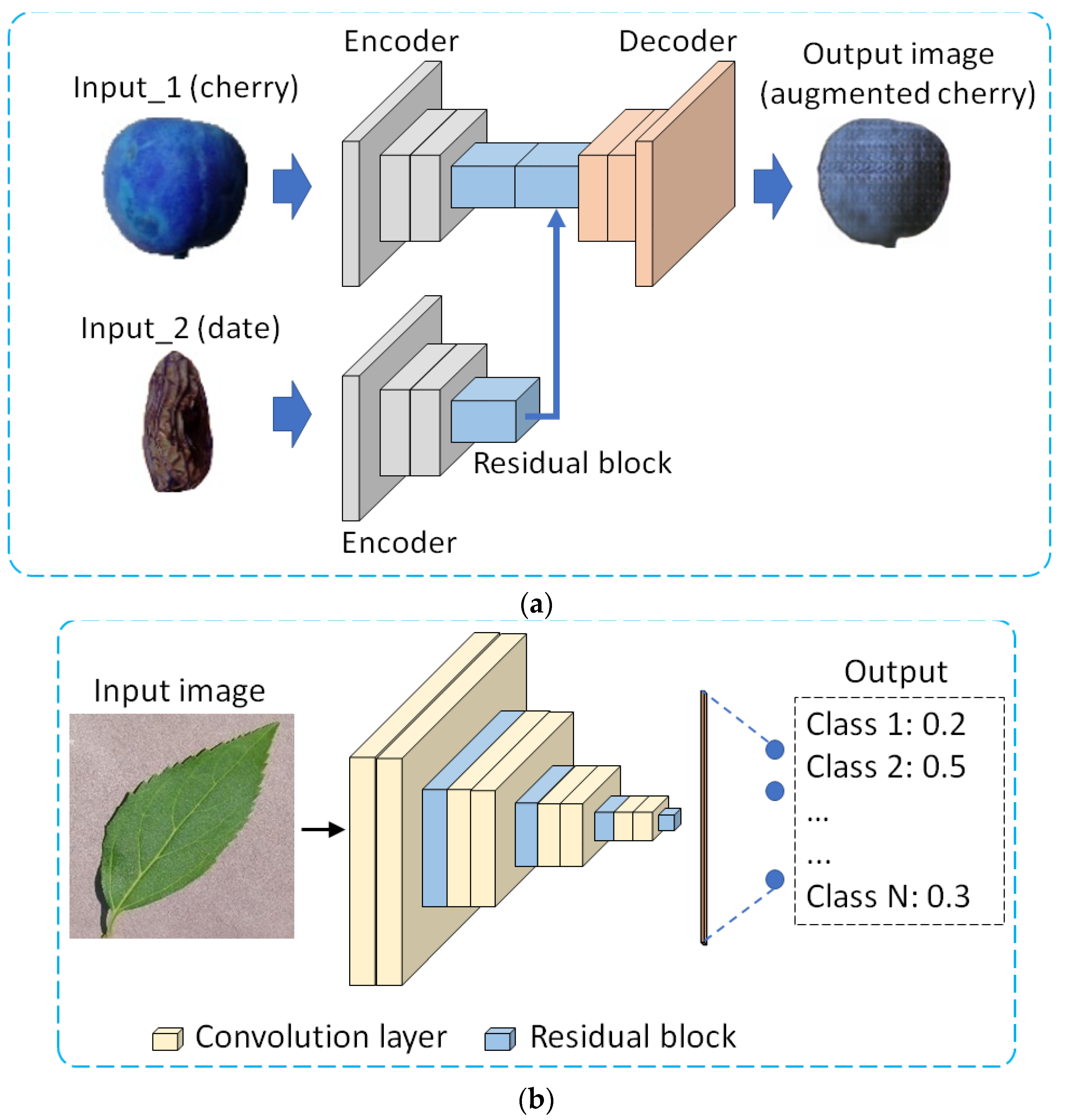
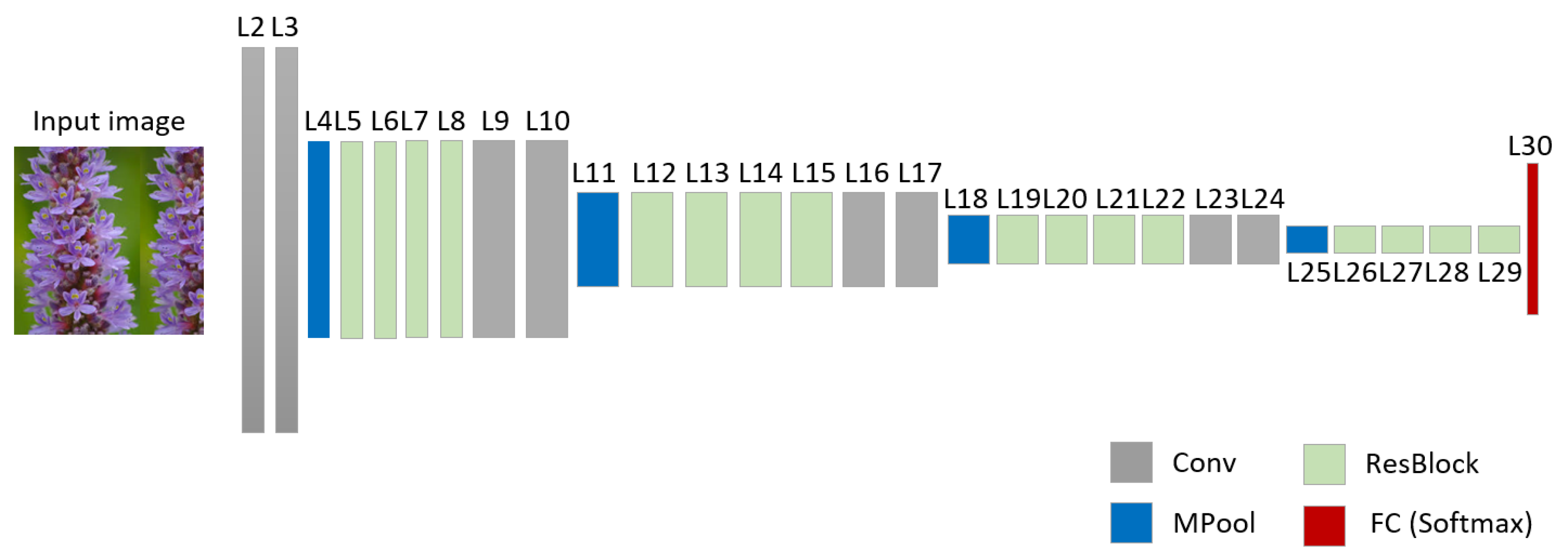
The proposed methods are explained in detail in this section. Figure 1 shows the flowcharts of the methods. As shown in Figure 1a, image augmentation by PI-GAN involves the use of two types of input images (different plant images) to augment plant images. Moreover, as shown in Figure 1b, the concepts of the visual geometry group network (VGG-Net) [26] and residual network (ResNet) [29] were combined for plant image classification by the PI-CNN proposed in this study. The size of input images and number of output classes vary across the four datasets used in this study. For example, the size of an input image in Figure 1a is 100 × 100 × 3 pixels, whereas the output of PI-GAN is 100 × 100 × 3 pixels. Furthermore, the size of an input image in Figure 1b is 256 × 256 × 3 pixels, whereas the output class of PI-CNN is 14. As shown in Figure 1a, the augmented plant image is used for training PI-CNN in Figure 1b.
3.2. Detailed Structure of Proposed PI-GAN and PI-CNN
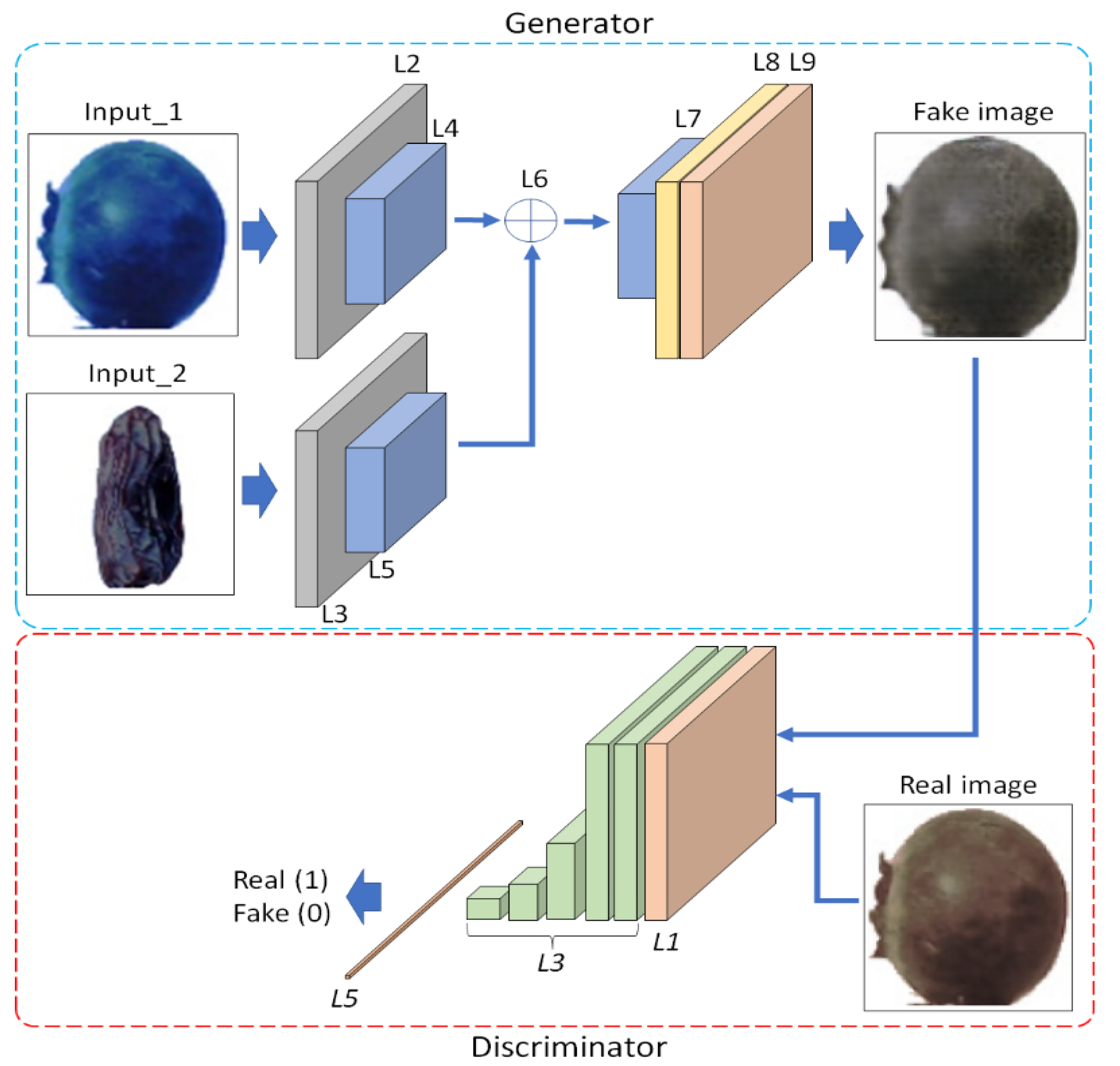
The detailed structure of the PI-GAN proposed in this study is presented in Table 2, Table 3, Table 4, Table 5, Table 6 and Table 7 and Figure 2. The generator and discriminator networks of the PI-GAN method are shown in Table 2 and Table 6. Furthermore, Table 8 and Figure 3 explain the proposed PI-CNN structure in detail. The structure shown in Table 2, Table 3, Table 4, Table 5, Table 6, Table 7 and Table 8 includes the input layer (input_layer), convolutional layer (conv2d), max pooling layer (max_pool), encoder block (encoder), decoder block (decoder), concatenate layer (concat), residual block (res_block), rectified linear unit (lrelu), parametric rectified linear unit (prelu), up sampling layer (Up2), additional operation layer (add), discriminator block (disc_block), and fully connected layer (FC). Furthermore, tanh and sigmoid represent activation functions. The stride and padding in Table 2, Table 3, Table 4 and Table 5 are (1 × 1) and (1 × 1), respectively. Meanwhile, the padding in Table 6 and Table 7 is (1 × 1). The input of a generator network is a 100 × 100 × 3 plant image, as shown in Figure 2, whereas the output is a 100 × 100 × 3 augmented plant image. The input of a discriminator network is a 100 × 100 × 3 plant image as in Figure 2, whereas the output is 1 × 1. In addition, a 100 × 100 × 3 image is used as an input of the proposed PI-CNN, whereas the output comprises 14 × 1 probabilities. The number of classes of output in Table 6 and Table 8 is 2 and 14, respectively. However, as explained in Section 3.3, the size of an input image in Table 2, Table 6, and Table 8 varies across the four types of datasets used in this study. Furthermore, the number of classes of output in Table 6 and Table 8 vary. The “Times” columns in Table 2 and Table 6 indicate the number of times each layer is used.
3.3. Dataset and Experimental Setup
In this study, the experiments were conducted using the PlantVillage dataset [15], PlantDoc dataset [16], Fruits-360 dataset [17], and Plants dataset [18]. The datasets comprise images of plants, fruits, and plant diseases acquired in different environments. The Fruits-360 dataset is composed of manually cropped images. The size and depth of the images are 100 × 100 × 3 pixels and 24 bits, respectively. The total number of images in the train and test sets are 41,322 and 13,877, respectively. Here, the test set is divided again to test and validation sets, and the number images of the test and validation sets are 12,877 and 1000, respectively. The PlantVillage dataset is also composed of manually cropped images. The size and depth of the images are 256 × 256 × 3 pixels and 24 bits, respectively. The total number of images is 54,305. Here, the dataset is divided to train, test, and validation sets, and each has 40,000, 13,305, and 1000 images, respectively. The PlantVillage dataset includes grayscale images and segmented images. The PlantDoc dataset is composed of manually cropped and original images. The size of images varies significantly: the smallest and largest sizes are 150 × 150 × 3 and 5616 × 3744 × 3, respectively. The depth of images is 24 bits. The total number of images in the train and test sets are 2336 and 236, respectively. Here, the test set is divided again to test and validation sets, and the number images of the test and validation sets are 200 and 36, respectively. The Plants dataset is composed of manually cropped and original images. The depth and size of the images are similar to those for the PlantDoc dataset. This dataset consists of a training set, a test set, and validation sets, and each contains 13,149, 5218, and 1521 images, respectively. The above-mentioned information is summarized in Table 9.
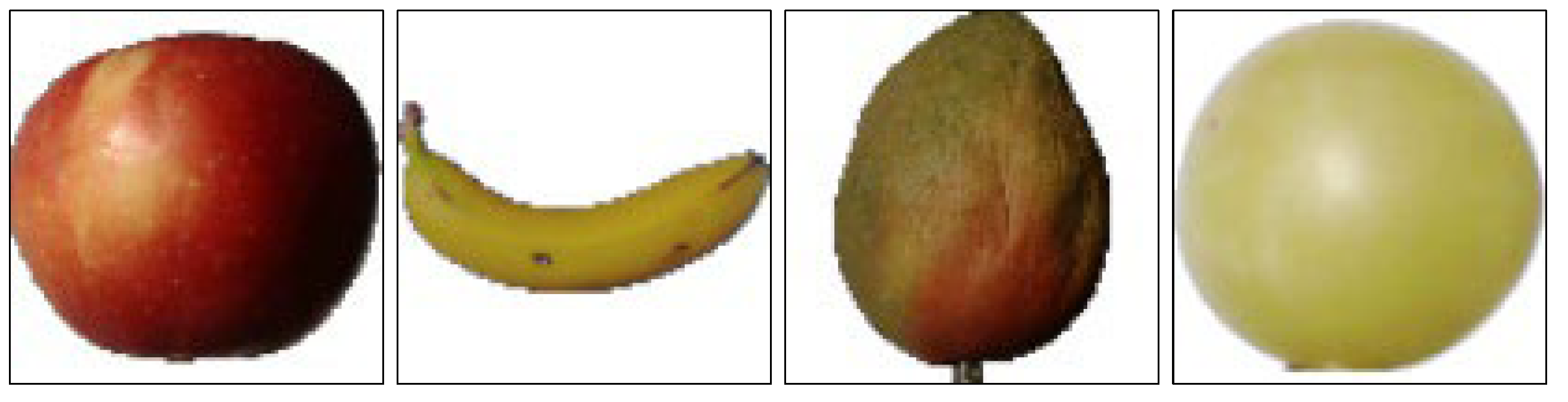
Figure 4, Figure 5, Figure 6 and Figure 7 show example images of the Fruits-360 dataset, PlantDoc dataset, PlantVillage dataset, and Plants dataset.
The process of training and testing both image augmentation and classification algorithms was performed using a desktop computer equipped with an Intel Core i7-6700 [email protected] GHz, an Nvidia GeForce GTX TITAN X graphics processing unit (GPU) card [30], and a random-access memory (RAM) of 32 GB. The proposed model and algorithm were implemented using OpenCV library (version 4.3.0) (Intel Corporation, CA, USA) [31], Python (version 3.5.4) (Rossum, G.V., DE, USA) [32], and the Keras application programming interface (API) (version 2.1.6-tf) (Chollet, F., CA, USA) with a TensorFlow backend engine (version 1.9.0) (Google, CA, USA) [33].
3.4. Data Augmentation
In this subsection, the augmented images obtained through the proposed plant-image augmentation method are explained in detail. As shown in Figure 2, when two images are input into PI-GAN and the features of input_2 are mixed with input_1 by using channel-wise concatenation as Layer 6 in Table 2 and L6 in Figure 2, a new image is generated through a decoder. The classification results were compared by conducting experiments wherein the number of images in the training set was increased from 70% to 100%, from 50% to 100%, from 30% to 100%, and from 10% to 100%. The experiments were conducted to compare the conventional augmentation methods and the PI-GAN-based augmentation methods. For example, a reduction in the total number of images in the training sets of the four datasets explained in Table 10 and Section 3.3 (Fruits-360 dataset: 41,322, PlantVillage dataset: 40,000, PlantDoc dataset: 2336, and Plants dataset: 13,149) by 70% results in 28,926, 28,000, 1635, and 9204 images, respectively. Furthermore, a reduction by 50% results in 20,661, 20,000, 1168, and 6574 images, respectively; a reduction by 30% results in 12,396, 12,000, 700, and 3944 images, respectively; and a reduction by 10% results in 4132, 4000, 233, and 1314 images, respectively.
The reduced training sets were augmented back to 100% (41,322, 40,000, 2336, and 13,149) through conventional augmentation methods (shifting in eight directions, in-plane rotation, flipping, blurring, scaling, brightness, and contrast). The training datasets were also augmented to 100% through the PI-GAN-based method. The PlantVillage and PlantDoc datasets were divided further into disease and crop sub-datasets in the experiment. Furthermore, training was performed by combining the training sets of the Plants and PlantDoc datasets (the numbers with ‘*’ in Table 11) in the training phase. Thus, the numbers of train subsets and test subsets are four (Fruits-360, PlantVillage crop, PlantVillage disease, and PlantDoc crop + PlantDoc disease + Plants) and six (Fruits-360, PlantVillage crop, PlantVillage disease, PlantDoc crop, PlantDoc disease, and Plants), respectively, as in Table 11.
Furthermore, training subsets of the original datasets, reduced datasets, datasets augmented by the conventional method, and datasets augmented by PI-GAN were constructed. The numbers of training subsets are 4 (100% of Fruits-360, PlantVillage crop, PlantVillage disease, and Plant), 16 (70%, 50%, 30%, and 10% of the four training subsets), 16 (70%, 50%, 30%, and 10% of the subsets were increased to 100%, 100%, 100%, and 100% of them by the conventional method), and 16 (70%, 50%, 30%, and 10% of the subsets were increased to 100%, 100%, 100%, and 100% of them by PI-GAN), respectively. Thus, the total number of training subsets is 52, whereas the total number of test subsets is 6. Detailed explanations are presented in Table 10 and Table 11.
In this study, the results from the original four training subsets (six test subsets) and the reduced 16 training subsets (6 test subsets) are compared in Section 4.2.1. In addition, the results obtained by augmenting the reduced datasets through conventional augmentation methods (16 training subsets and 6 test subsets) and through PI-GAN-based augmentation methods (16 training subsets and 6 test subsets) are compared in Section 4.2.2 and Section 4.2.3, respectively.
4. Experimental Results
This section is divided into four subsections. These address the training setup, ablation study, comparisons with the state-of-the-art methods, and processing time. The training setup of the training phase such as hyperparameters and training loss are explained in Section 4.1. The results obtained from the ablation study are presented in Section 4.2. Furthermore, Section 4.2.1 compares the classification results by using 30 sub-datasets of different sizes, Section 4.2.2 compares the classification results by using 24 datasets augmented through conventional augmentation methods, and Section 4.2.3 compares the classification results by using 24 datasets augmented through the GAN-based augmentation methods. Section 4.3 compares the experimental results of 78 datasets obtained through the existing plant-image classification methods and the proposed method. Finally, the processing time is recommended in Section 4.4.
4.1. Training Setup
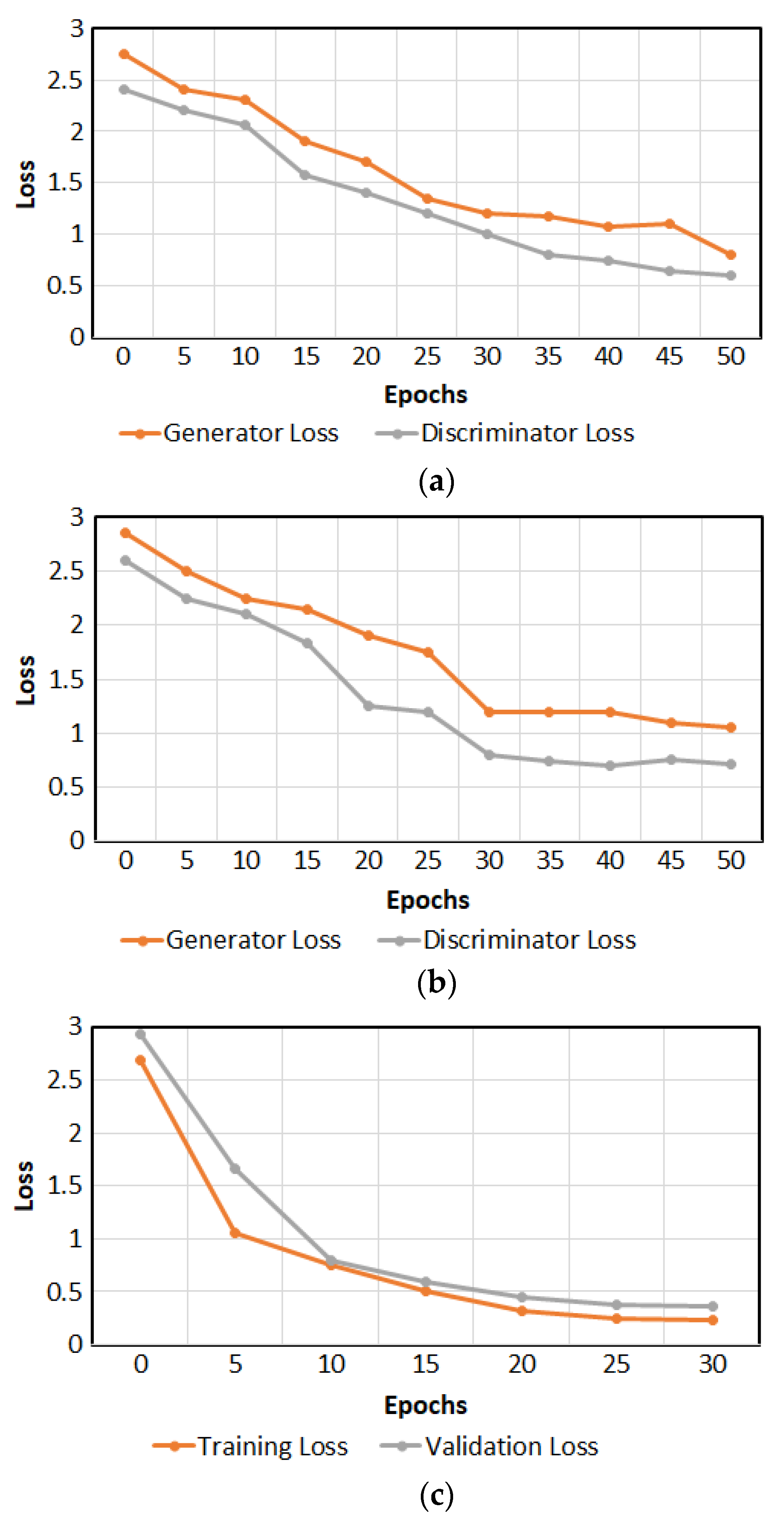
The training setups of the PI-GAN-based plant image augmentation method and proposed PI-CNN-based plant image classification method were as follows. The batch size, training epoch, and learning rate were set to 8, 50, and 0.0001 for the PI-GAN and to 8, 40, and 0.0001 for the PI-CNN, respectively. Moreover, we used the binary cross-entropy loss [34] for both generator and discriminator losses and used the categorical cross-entropy loss [35] for the PI-CNN loss. Adaptive moment estimation (Adam) [36] was used as an optimizer in both PI-CNN and discriminator networks. Figure 8a,b show the training loss and validation loss curves of the proposed PI-GAN per epoch, respectively, whereas Figure 8c,d show the training and validation loss and accuracy curves of the proposed PI-CNN per epoch, respectively. As shown by the convergences of the training loss and accuracy curves in Figure 8, the proposed PI-GAN and PI-CNN were trained sufficiently with the training data. Furthermore, as shown by the convergences of the validation loss and validation accuracy curves in Figure 8, the proposed PI-GAN and PI-CNN are not overfitted to the training data. Table 12 and Table 13 show the search spaces and selected values of hyperparameters for PI-GAN and PI-CNN.
4.2. Ablation Study
The results of various ablation studies are presented in this subsection. The accuracy of the plant classification was measured using four types of metrics in Equations (1)–(4). Here, the true positive rate (TPR), positive predictive values (PPV), accuracy (ACC) [37], and F1-score [38] are presented. In the equations given below, TP, FP, FN, and TN refer to true positive, false positive, false negative, and true negative, respectively. Here, “#” indicates “the number of”.
4.2.1. Plant Image Classification
In this subsection, we conducted experiments to obtain a good generator structure for PI-GAN, and to obtain a classification structure for PI-CNN. Four different generator networks were compared by using Fruits-360 dataset and PI-CNN, as shown in Table 14. Moreover, four different networks were compared for PI-CNN by using Fruits-360 dataset and without using PI-GAN, as shown in Table 15. As shown in Table 14, a generator network with four encoder-decoders showed higher accuracy compared to others. Moreover, as shown in Table 15, a network with sixteen residual blocks showed higher accuracy compared to others. Therefore, we used a generator network with four encoder-decoders for PI-GAN and a network with sixteen residual blocks for PI-CNN.
In addition, four training sub-datasets (PlantVillage disease, PlantVillage crop, PlantDoc disease + PlantDoc crop + Plants, and Fruits-360) were divided further according to five sizes (100%, 70%, 50%, 30%, and 10%), as explained in Section 3.4, to train the image classification models. The classification accuracy was measured using six testing sub-datasets (PlantVillage disease, PlantVillage crop, PlantDoc disease, PlantDoc crop, Plants, and Fruits-360). The results are compared in Table 16, Table 17 and Table 18. As shown in these tables, the classification accuracy decreases as the size of the training dataset decreases.
4.2.2. Plant Image Classification with Conventional Image Augmentation Methods
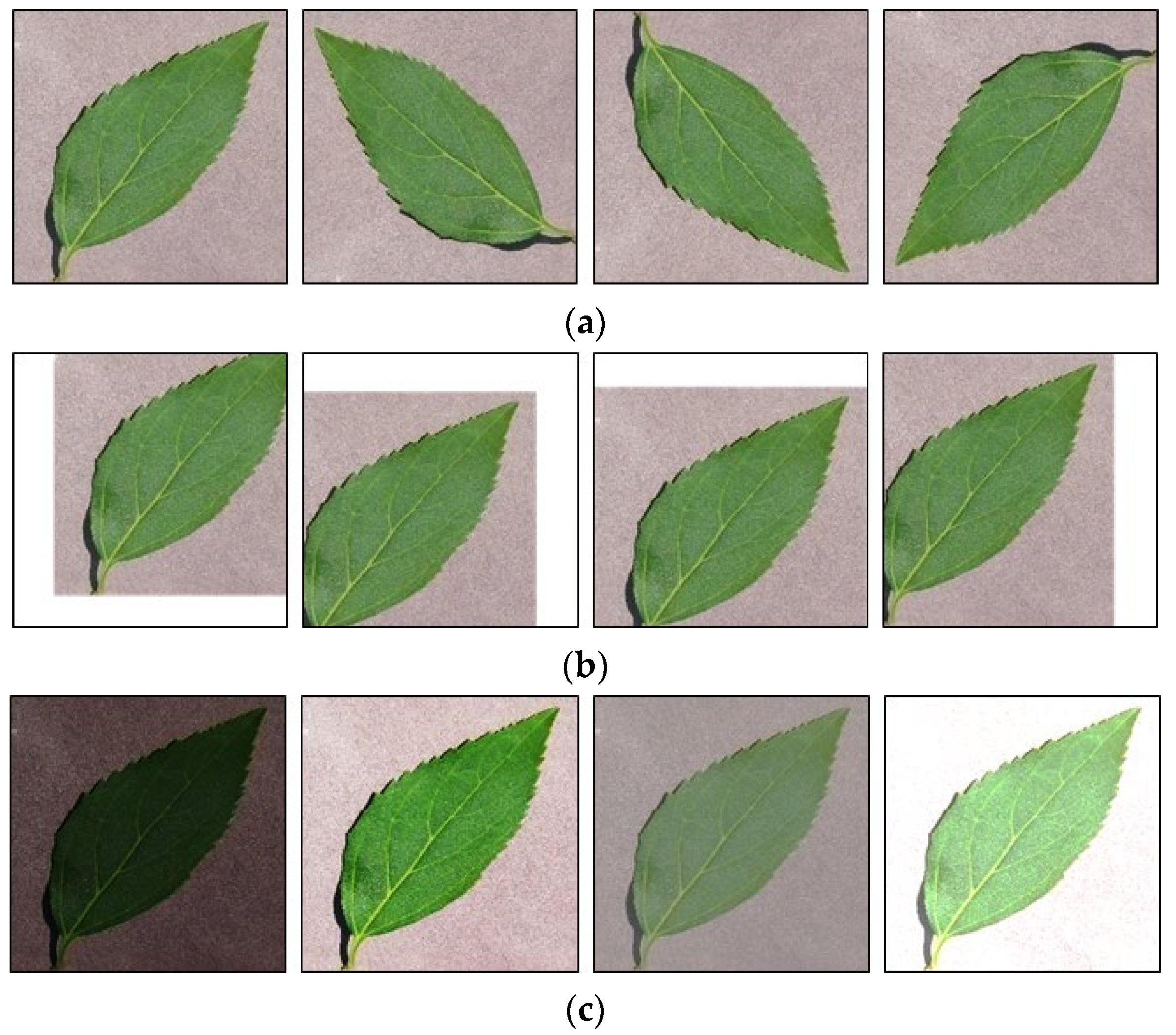
In this subsection, image classification was repeated using the training datasets augmented through conventional augmentation methods (image shifting to four directions, in-plane rotation, flipping, Gaussian blurring, scaling, and the adjustments of brightness and contrast) to improve the classification accuracy. Figure 9 shows an example of augmented image data. The results of the experiments are compared in Table 19, Table 20 and Table 21.
Additionally, we conducted experiments using random cropping [45] for augmentation and showed the results in Table 22, Table 23 and Table 24. A comparison between Table 19, Table 20, Table 21, Table 22, Table 23 and Table 24 and Table 16, Table 17 and Table 18 reveals that the augmentation improved the classification accuracy.
4.2.3. Plant Image Classification with PI-GAN-Based Augmentation Methods
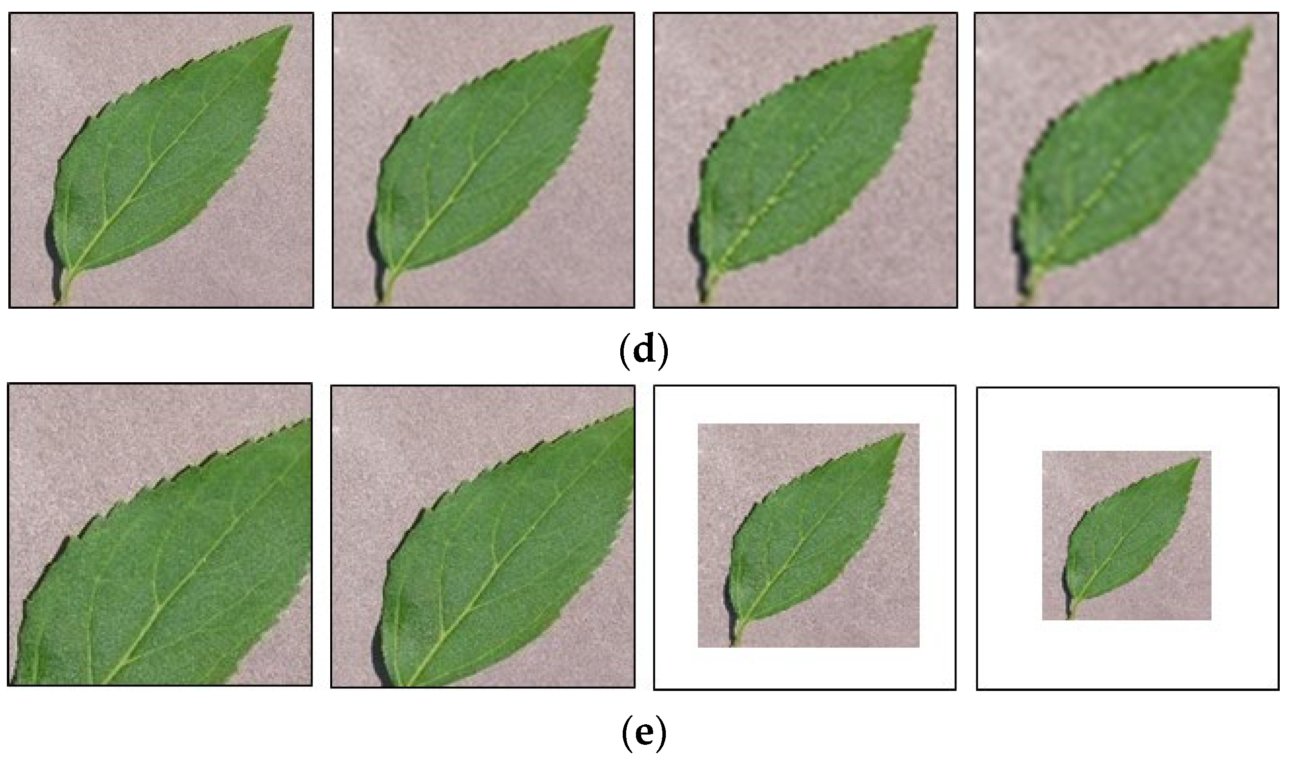
In this subsection, image classification was performed using the training datasets augmented back by the PI-GAN-based augmentation method to improve the classification accuracy shown in Table 16, Table 17 and Table 18. Figure 10 shows an example of augmented image data. The results of the experiments are compared in Table 25, Table 26 and Table 27. A comparison of these tables with Table 16, Table 17 and Table 18 reveals that the augmentation improved the classification accuracy.
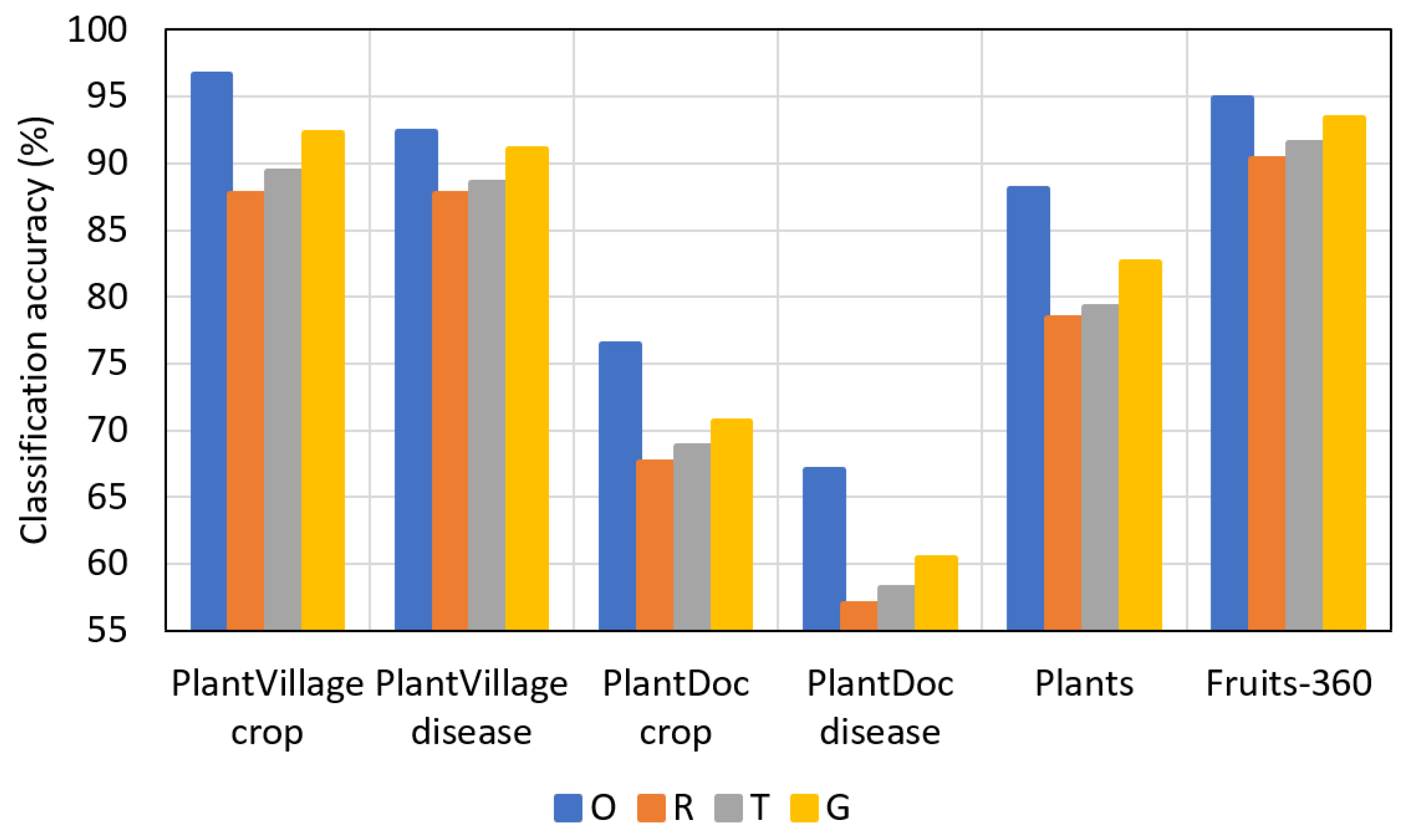
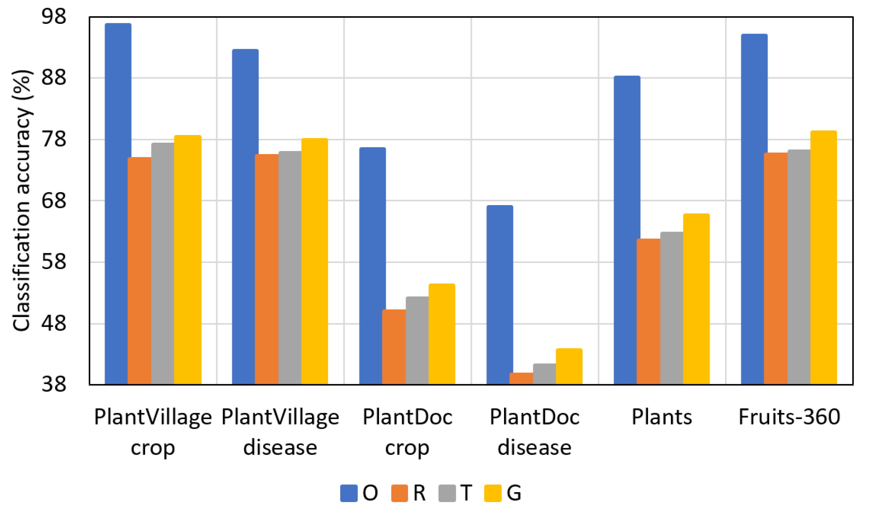
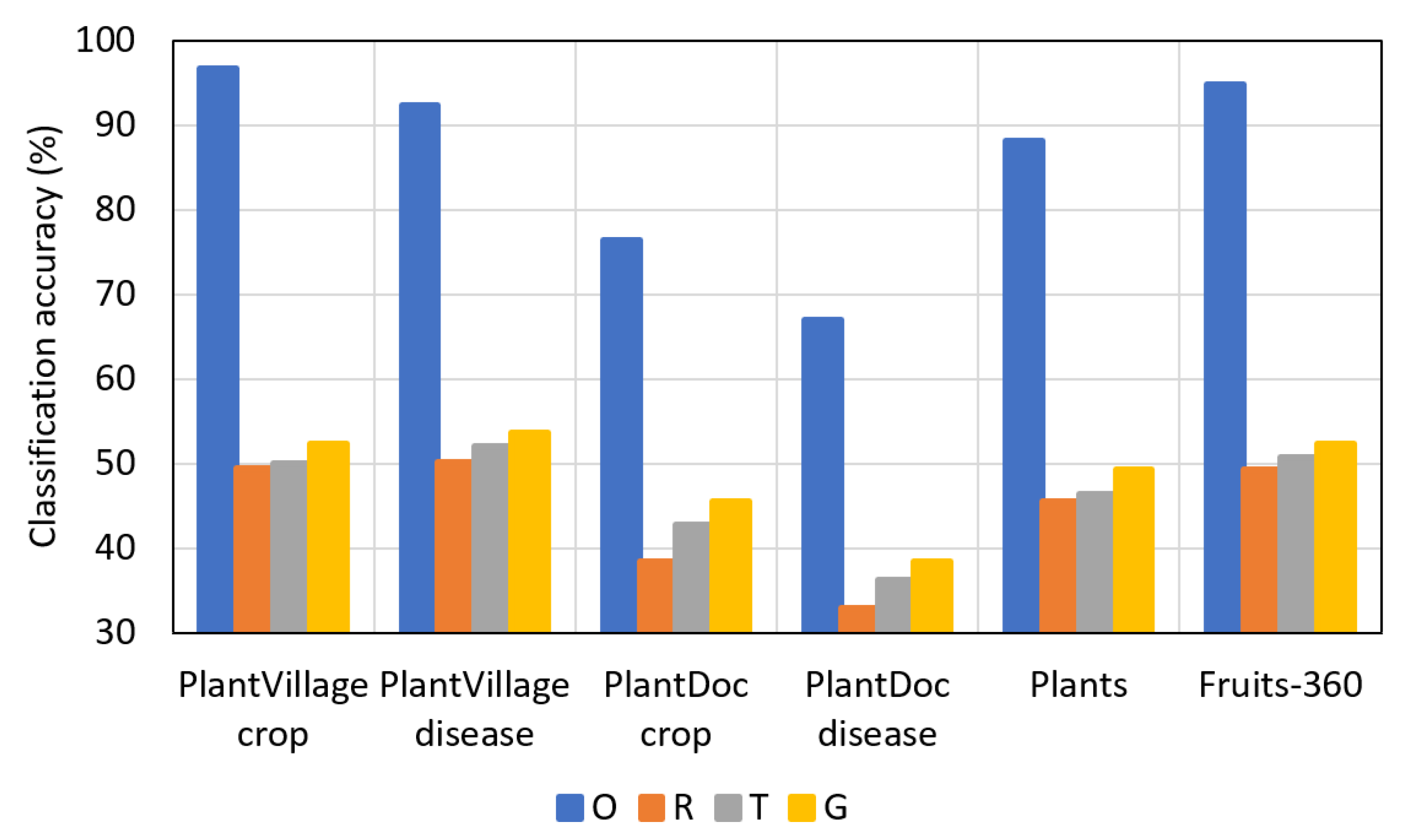
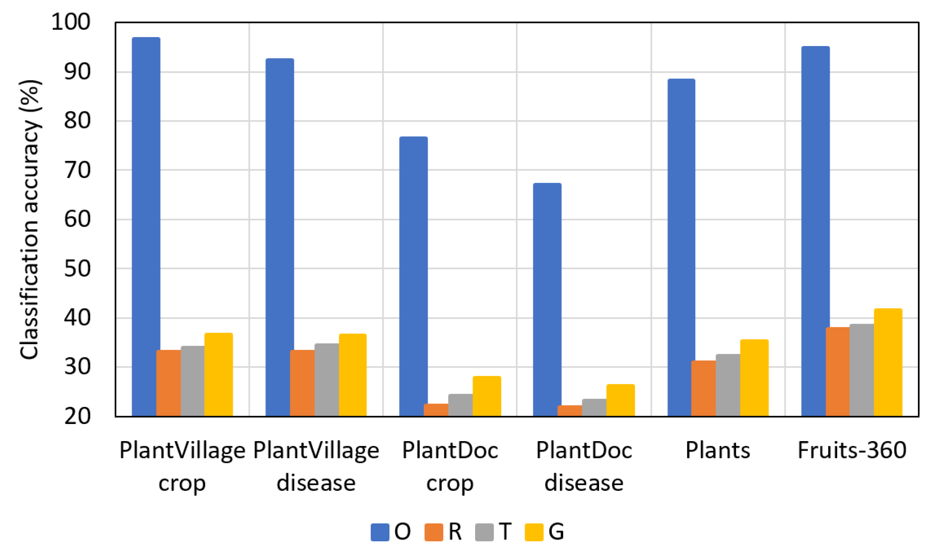
Figure 11, Figure 12, Figure 13 and Figure 14 present a comparison of F1-scores between the reduced datasets and augmented datasets conveniently. The results in the figures are presented in the following order (top to bottom): original dataset (O), reduced dataset (R), dataset augmented by conventional method (T), and dataset augmented by PI-GAN (G).
As shown in Figure 11, Figure 12, Figure 13 and Figure 14, lower F1-scores were obtained when the reduced datasets were used, whereas higher F1-scores were obtained when the datasets augmented by conventional methods were used. Furthermore, higher F1-scores were obtained when the datasets augmented by PI-GAN-based methods were used. In Table 28, Table 29 and Table 30, the existing augmentation method [46] based on conditional GAN is used to perform the classification for additional experiments. As shown in Table 25, Table 26, Table 27, Table 28, Table 29 and Table 30, classification accuracies by using the proposed PI-GAN are higher compared to those using the existing method [46].
As shown in Table 16, Table 17 and Table 18, we achieved higher accuracy when using a bigger dataset. Moreover, we achieved higher accuracy when using image augmentation, as shown in Table 19, Table 20, Table 21, Table 22, Table 23, Table 24, Table 25, Table 26, Table 27, Table 28, Table 29 and Table 30. Thus, increasing the size of the dataset will not be detrimental to PI-CNN.
4.3. Comparisons with State-of-the-Art Methods
4.4. Processing Time
The processing time of the PI-GAN method and classification method (PI-CNN) in the testing phase is shown in Table 34. The processing time was measured in the environments explained in Section 3.3. As shown in Table 34, the frame rate of the PI-GAN method is approximately 21.78 frames per second (fps) (=1000/45.92). Moreover, the frame rate of the proposed PI-CNN is approximately 19.29 fps (=1000/51.85). The total frame rate including both image augmentation and classification method is approximately 10.23 fps (1000/97.77).
5. Discussion
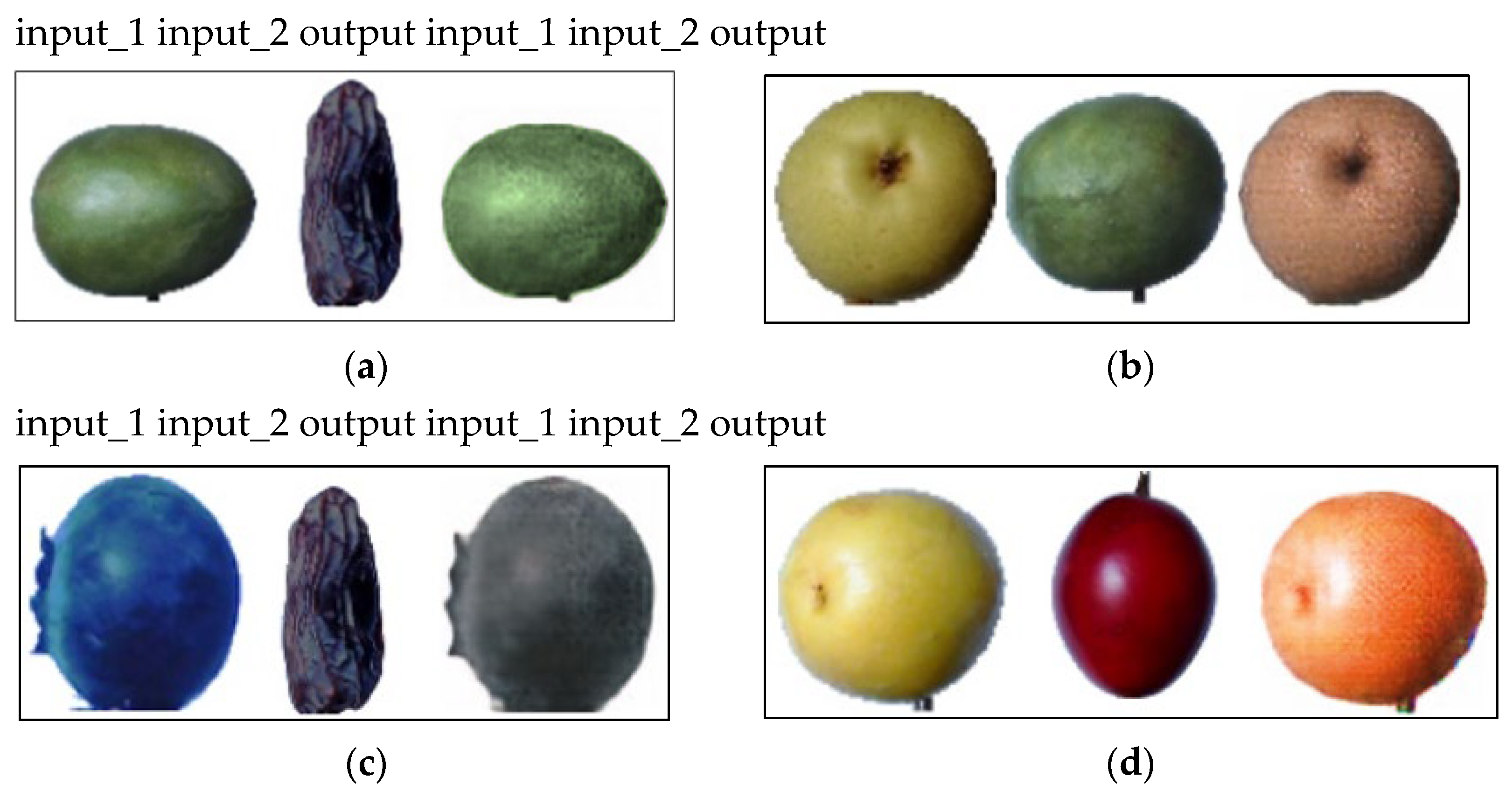
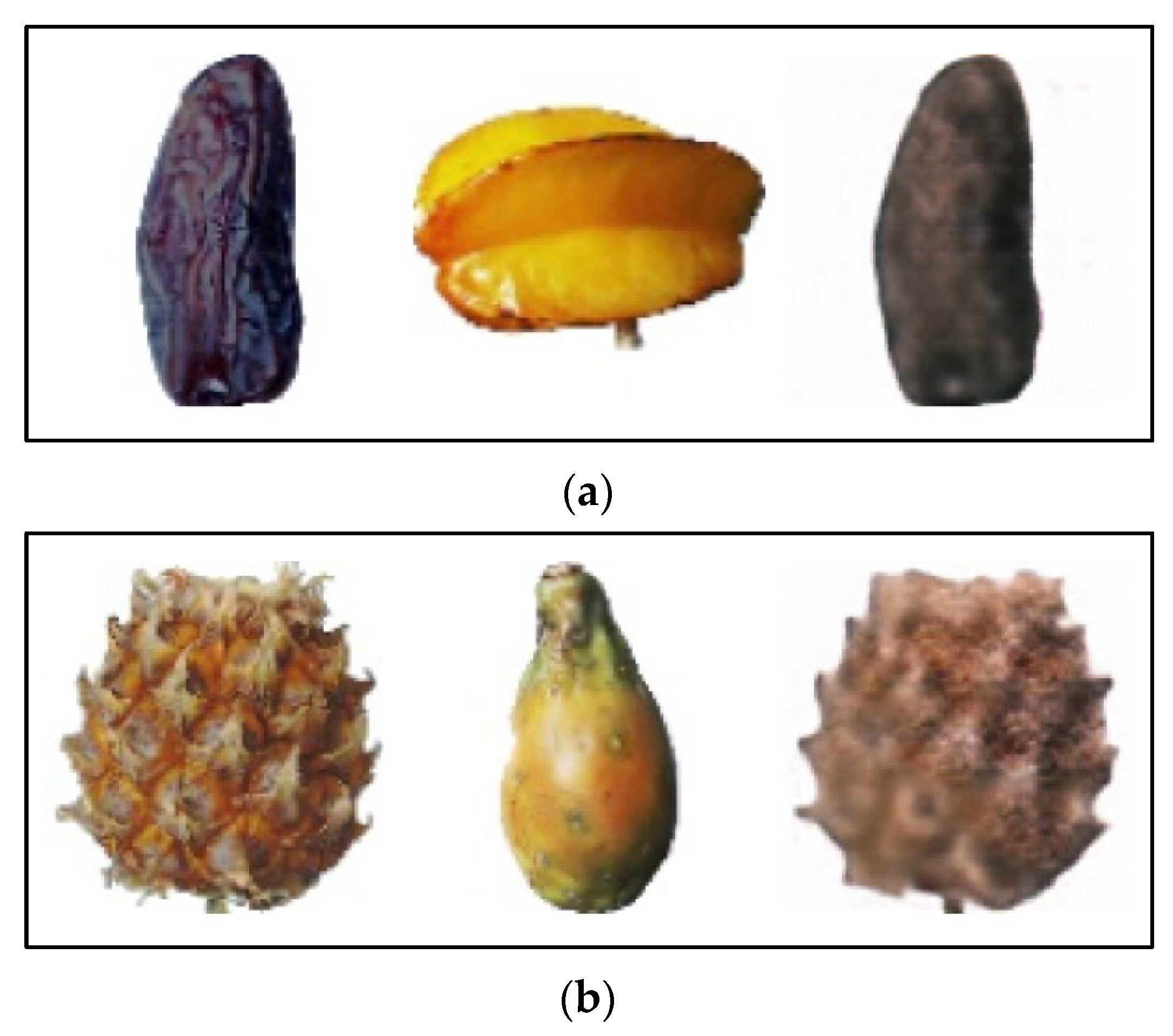
In general, the plant-image classification performance is affected by the structure of the classification model, as well as the image quality and number of images in the datasets. Existing plant-image open datasets are typically small in size compared with open datasets of other fields. Furthermore, only a small number of open datasets exist. Therefore, previous models trained using a small number of plant images demonstrate a lower classification accuracy. This study verified that image classification performed using a small number of training images yielded a lower classification accuracy as the number of images decreased. Accordingly, experiments were conducted in this study by increasing the number of images by using the augmentation method involving PI-GAN. The experimental results obtained with four open databases demonstrated that the classification accuracy was improved compared with those of the state-of-the-art methods for all the reduced datasets. However, there are error cases when augmenting images using PI-GAN, as shown in Figure 15. For example, augmented image is presented in Figure 15a, where the date, carambula, and augmented date image are presented. In the case of the augmented date image, the pattern of the date in the image was lost and looks more like a rock. Moreover, as shown in Figure 15b, pineapple, cactus fruit, and augmented pineapple are presented. Here, the augmented pineapple image became blurry. These errors arise because the two input images are only combined by using a channel-wise concatenation operation rather than by analyzing a pattern style of an input image and applying the pattern style of one image to another input image.
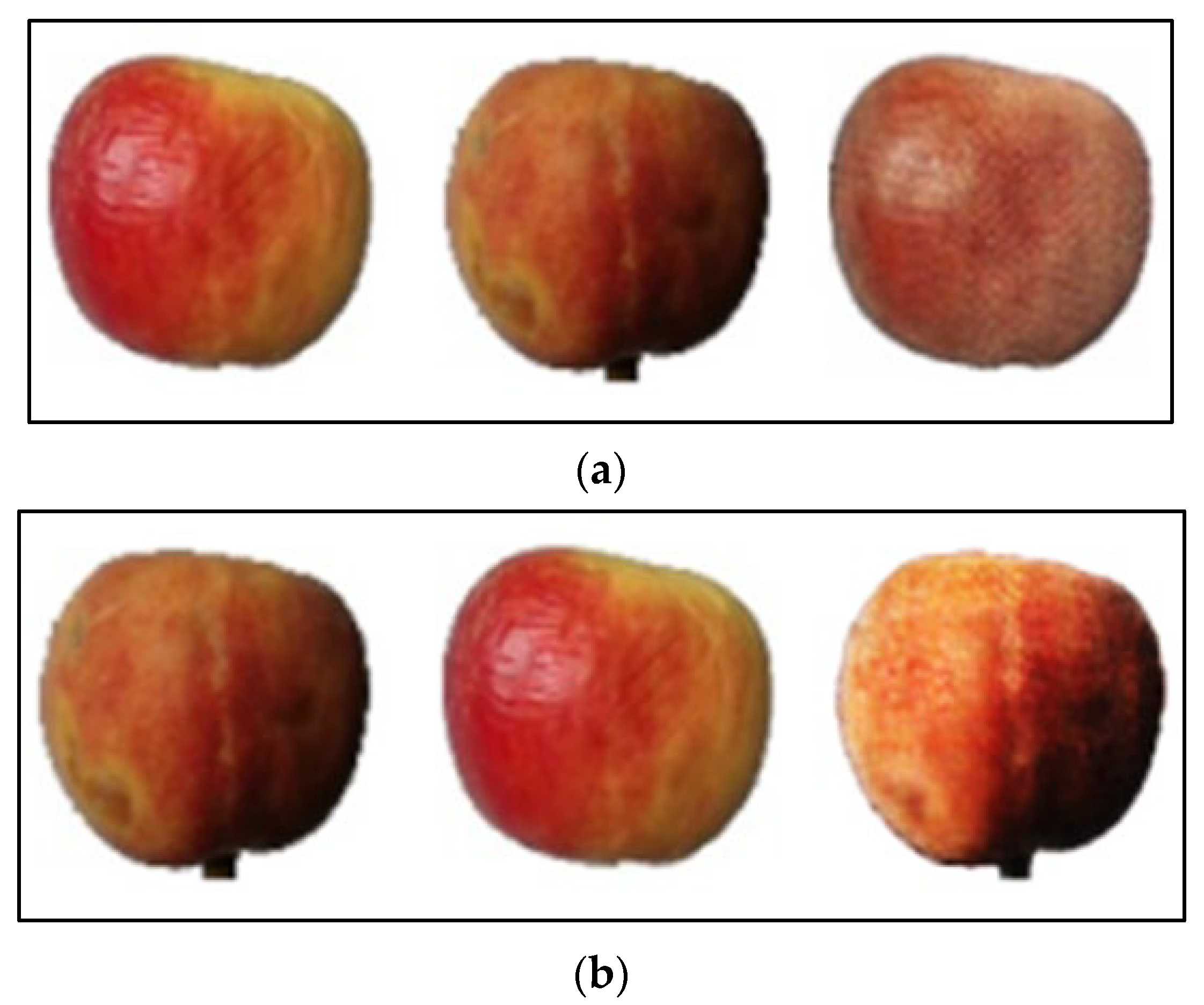
Moreover, example images misclassified by the proposed PI-CNN are presented in Figure 16. For example, apple, peach, and augmented apple images are presented from the left to right in Figure 16a, and peach, apple, and augmented peach images are presented in the same way in Figure 16b. In case of Figure 16a, an apple image (input_1) is augmented based on a peach image (input_2). Thus, the augmented apple (output) image looks a little bit like a peach image. On the contrary, a peach image (input_1) is augmented based on an apple image (input_2) in Figure 16b. So, the augmented peach image looks similar to the apple image. That is, the classification errors occur due to the loss of class information in the augmented images used for the training of PI-CNN in both Figure 16a,b.
We obtained the PI-GAN and PI-CNN structures based on experimental results through ablation studies (Section 4.2). For the model structure adjustment and optimization for the specific domain of plant images, we conducted experiments by using various parameters (Table 12 and Table 13) and structures (Table 14 and Table 15).
Compared to previous GAN-based image augmentation methods [47,48,49], the proposed PI-GAN is novel as follows:
- -
- -
- -
- -
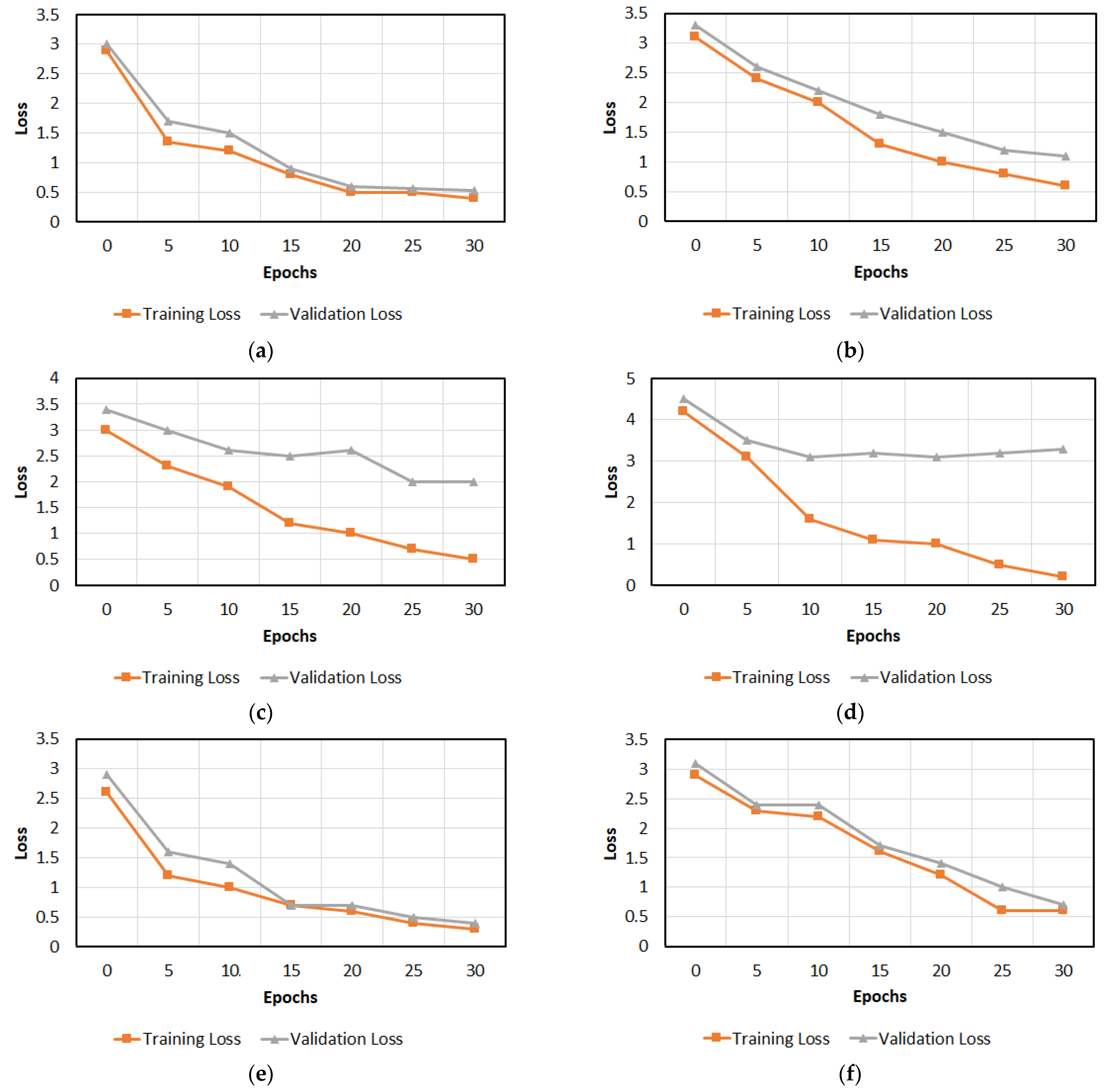
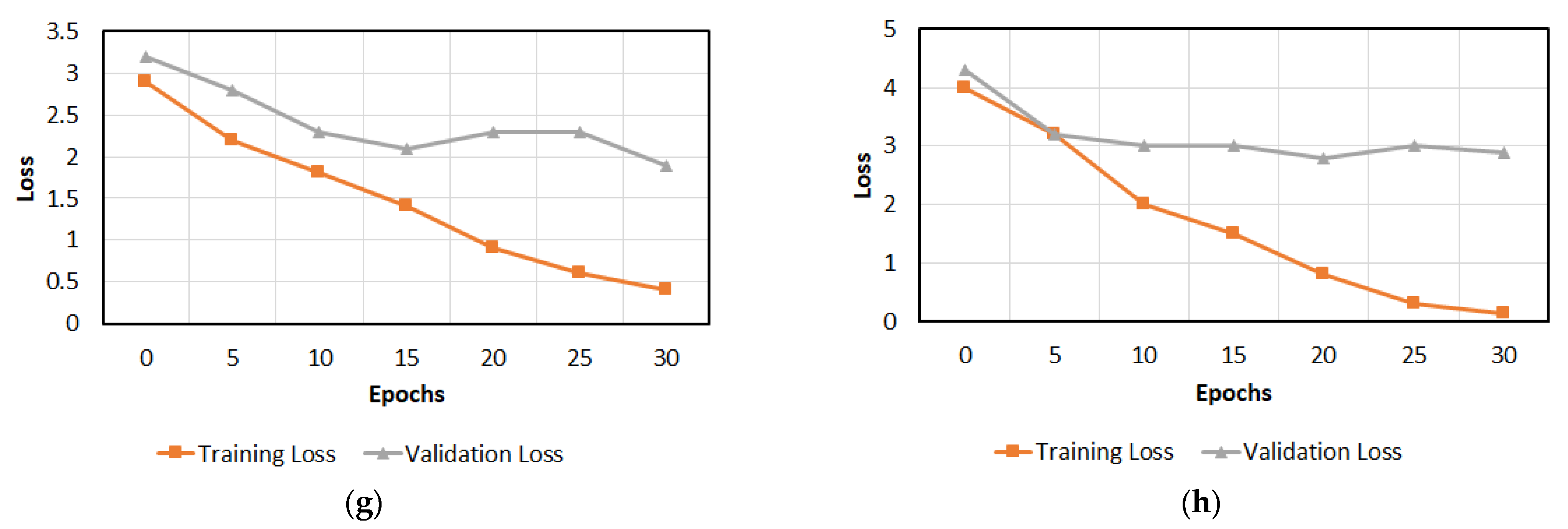
Using a small dataset causes the overfitting problem. In the training phase, we can monitor overfitting based on the curves of the loss of validation dataset. For example, we can identify overfitting when validation loss stops decreasing after a certain number of training epochs while the training loss keeps decreasing. The overfitting occurs in cases where the training metric keeps searching for the best fit only for the training dataset. The solution to overcome the overfitting is to increase the number of training data.
In this paper, we conducted various experiments by using training datasets with different sizes. Training and validation loss curves of the experiments are presented in the following figures to determine whether the models were overfitted.
As shown in Figure 17d, the training loss is decreased more than those in Figure 17a–c. This is because the number of training images is too small in Figure 17d, and the model is fitted easily. However, the validation loss in Figure 17d is not decreased after epoch 10, which confirms overfitting caused by a small training set. Similarly, overfitting occurs in Figure 17c owing to the same reason. The testing accuracies with the augmented data of Figure 17g,h become higher than those with the original data of Figure 17c,d as shown in Table 25, Table 26 and Table 27. In addition, the validation losses with the augmented data of Figure 17g,h are a little lower than those with the original data of Figure 17c,d.
There have been various experiments conducted based on different numbers of parameters and layers [26,29]. As shown in [29], the error rates by the CNN model usually increase when the number of layers and parameters decrease. The experimental results with VGG Net in [26] confirm that the error rates by the CNN model usually increase when the number of layers decrease. Therefore, we confirm that other conventional CNN models usually achieve worse results by reducing the parameters.
6. Conclusions
This study proposed plant-image augmentation and classification methods and performed various experiments. New plant images were obtained by combining two types of input plant images in the plant image augmentation by PI-GAN. The proposed classification by PI-CNN involved the classification of images using augmented and original images. Moreover, the accuracy in a case where a small number of training datasets were used was compared with that in a case where a large number of training datasets were used. The size of the original dataset was set to 100%, and the dataset size was reduced by 70%, 50%, 30%, and 10% to compare the difference in accuracy. Subsequently, the accuracy was compared again by augmenting the training datasets that had been reduced by 70%, 50%, 30%, and 10%, back to 100%, using conventional and PI-GAN-based augmentation methods. As shown in Table 25, Table 26 and Table 27, classification accuracies obtained by using the proposed PI-GAN augmentation method are higher compared to those obtained by using conventional data augmentation methods as in Table 19, Table 20, Table 21, Table 22, Table 23 and Table 24. This confirms that the proposed PI-GAN outperforms the conventional augmentation methods. To augment a plant image, the proposed PI-GAN extracts feature from two different plant images and combines them to generate a new plant image, whereas conventional augmentation methods change a plant image by in-plane rotation, shifting, flipping, and adjustments of brightness and contrasts to generate different images. In addition, as shown in Table 25, Table 26 and Table 27, classification accuracies obtained by using PI-CNN with PI-GAN are higher compared to those obtained by using PI-CNN with conventional augmentation methods. Moreover, classification accuracies obtained by using PI-CNN with PI-GAN are higher compared to those obtained by using PI-CNN with the existing conditional GAN-based method [46], as shown in Table 28, Table 29 and Table 30. This confirms that the proposed PI-GAN works better with the proposed PI-CNN. The results of the experiments performed using four open datasets (namely, PlantDoc, PlantVillage, Plants, and Fruits-360) verified that the proposed PI-GAN and PI-CNN achieved a high classification accuracy compared with the state-of-the-art methods in all the cases.
In future studies, a variety of explainable artificial intelligence (XAI) methods [39,40,41,42,43,44] will be considered to examine the methods further to improve the accuracy of PI-CNN methods for image classification. In addition, we will conduct further research into methods for maintaining the class information in the augmented images in order to minimize the classification errors.
Author Contributions
Methodology, G.B.; validation, S.H.N.; supervision, K.R.P.; writing—original draft, G.B.; writing—review and editing, K.R.P. All authors have read and agreed to the published version of the manuscript.
Funding
This research was supported in part by the National Research Foundation of Korea (NRF) funded by the Ministry of Science and ICT (MSIT) through the Basic Science Research Program (NRF-2022R1F1A1064291), in part by the NRF funded by the MSIT through the Basic Science Research Program (NRF-2021R1F1A1045587), and in part by the NRF funded by the MSIT through the Basic Science Research Program (NRF-2020R1A2C1006179).
Institutional Review Board Statement
Not applicable.
Informed Consent Statement
Not applicable.
Data Availability Statement
Not applicable.
Conflicts of Interest
The authors declare no conflict of interest.
References
- Shahi, T.B.; Sitaula, C.; Neupane, A.; Guo, W. Fruit classification using attention-based MobileNetV2 for industrial applications. PLoS ONE 2022, 17, e0264586. [Google Scholar] [CrossRef] [PubMed]
- Siddiqi, R. Comparative performance of various deep learning based models in fruit image classification. In Proceedings of the 11th International Conference on Advances in Information Technology, Bangkok, Thailand, 1–3 July 2020; Volume 14, pp. 1–9. [Google Scholar] [CrossRef]
- Siddiqi, R. Effectiveness of transfer learning and fine tuning in automated fruit image classification. In Proceedings of the 2019 3rd International Conference on Deep Learning Technologies, Xiamen, China, 5–7 July 2019; pp. 91–100. [Google Scholar] [CrossRef]
- Savant, S.P.; Khanagoudar, P.S. Autonomous fruit recognition system based on deep convolutional neural network. Int. J. Sci. Res. Sci. Eng. Technol. 2020, 7, 666–669. [Google Scholar] [CrossRef]
- Srivastava, S.; Singh, T.; Sharma, S.; Verma, A. A fruit recognition system based on modern deep learning technique. Int. J. Eng. Res. Technol. 2020, 9, 896–898. [Google Scholar] [CrossRef]
- Biswas, B.; Ghosh, S.K.; Ghosh, A. A robust multi-label fruit classification based on deep convolution neural network. In Computational Intelligence in Pattern Recognition. Advances in Intelligent Systems and Computing; Das, A., Nayak, J., Naik, B., Pati, S., Pelusi, D., Eds.; Springer: Singapore, 2020; Volume 999. [Google Scholar] [CrossRef]
- Franczyk, B.; Hernes, M.; Kozierkiewicz, A.; Kozina, A.; Pietranik, M.; Roemer, I.; Schieck, M. Deep learning for grape variety recognition. Procedia Comput. Sci. 2020, 176, 1211–1220. [Google Scholar] [CrossRef]
- Hossain, M.S.; Al-Hammadi, M.; Muhammad, G. Automatic fruit classification using deep learning for industrial applications. IEEE Trans. Ind. Inform. 2019, 15, 1027–1034. [Google Scholar] [CrossRef]
- Hamid, N.N.A.A.; Razali, R.A.; Ibrahim, Z. Comparing bags of features, conventional convolutional neural network and AlexNet for fruit recognition. Indones. J. Electr. Eng. Comput. Sci. 2019, 14, 333–339. [Google Scholar] [CrossRef]
- Kader, A.; Sharif, S.; Bhowmick, P.; Mim, F.H.; Srizon, A.Y. Effective workflow for high-performance recognition of fruits using machine learning approaches. Int. Res. J. Eng. Technol. 2020, 7, 1516–1521. [Google Scholar]
- Katarzyna, R.; Paweł, M.A. Vision-based method utilizing deep convolutional neural networks for fruit variety classification in uncertainty conditions of retail sales. Appl. Sci. 2019, 9, 3971. [Google Scholar] [CrossRef] [Green Version]
- Ghosh, S.; Mondal, M.J.; Sen, S.; Chatterjee, S.; Kar Roy, N.; Patnaik, S. A novel approach to detect and classify fruits using ShuffleNet V2. In Proceedings of the IEEE Applied Signal Processing Conference, Kolkata, India, 7–9 October 2020; pp. 163–167. [Google Scholar] [CrossRef]
- Muhathir, M.; Santoso, M.H.; Muliono, R. Analysis naïve bayes in classifying fruit by utilizing HOG feature extraction. J. Inform. Telecommun. Eng. 2020, 4, 250–259. [Google Scholar] [CrossRef]
- Wang, D.; Wang, J.; Li, W.; Guan, P. T-CNN: Trilinear convolutional neural networks model for visual detection of plant diseases. Comput. Electron. Agric. 2021, 190, 106468. [Google Scholar] [CrossRef]
- PlantVillage Dataset. Available online: https://www.kaggle.com/datasets/emmarex/plantdisease (accessed on 5 July 2022).
- Singh, D.; Jain, N.; Jain, P.; Kayal, P.; Kumawat, S.; Batra, N. PlantDoc: A dataset for visual plant disease detection. In Proceedings of the 7th ACM IKDD CoDS and 25th COMAD, Hyderabad, India, 5–7 January 2020; pp. 249–253. [Google Scholar] [CrossRef]
- Fruits-360 Dataset. Available online: https://www.kaggle.com/datasets/moltean/fruits (accessed on 5 July 2022).
- Plants Dataset. Available online: https://www.kaggle.com/datasets/muhammadjawad1998/plants-dataset99-classes/metadata (accessed on 5 July 2022).
- Pawara, P.; Okafor, E.; Schomaker, L.; Wiering, M. Data augmentation for plant classification. In Proceedings of the Advanced Concepts for Intelligent Vision, Antwerp, Belgium, 18–21 September 2017; pp. 1–12. [Google Scholar] [CrossRef]
- Ghesquiere, M.; Ngxande, M. Deep learning for plant disease detection. In Advances in Computer Vision and Computational Biology; Springer International Publishing: Berlin/Heidelberg, Germany, 2021; pp. 69–84. [Google Scholar] [CrossRef]
- Image Data Augmentation. Available online: https://machinelearningmastery.com/how-to-configure-image-data-augmentation-when-training-deep-learning-neural-networks/ (accessed on 5 July 2022).
- Popular Image Augmentation Packages. Available online: https://www.kaggle.com/code/parulpandey/overview-of-popular-image-augmentation-packages/notebook (accessed on 5 July 2022).
- Santos, T.; Leonardo, D.S.; Andreza, D.S.; Sandra, A. Embrapa wine grape instance segmentation dataset—Embrapa WGISD (1.0.0) [Data set]. Zenodo 2019. Available online: https://zenodo.org/record/3361736#.Ywgs0nZByUk (accessed on 5 July 2022). [CrossRef]
- FIDS30 Dataset. Available online: https://www.kaggle.com/datasets/arnavmehta710a/fids30 (accessed on 5 July 2022).
- Szegedy, C.; Vanhoucke, V.; Ioffe, S.; Shlens, J.; Wojna, Z. Rethinking the inception architecture for computer vision. arXiv 2015, arXiv:1512.00567. [Google Scholar]
- Simonyan, K.; Zisserman, A. Very deep convolutional networks for large-scale image recognition. arXiv 2015, arXiv:1409.1556v6. [Google Scholar]
- Redmon, J.; Farhadi, A. Yolo V3: An incremental improvement. arXiv 2018, arXiv:1804.02767. [Google Scholar]
- PI-GAN and PI-CNN Models. Available online: https://github.com/ganav/PI-GAN-and-PI-CNN-networks (accessed on 5 July 2022).
- He, K.; Zhang, X.; Ren, S.; Sun, J. Deep residual learning for image recognition. In Proceedings of the IEEE Conference on Computer Vision and Pattern Recognition, Las Vegas, NV, USA, 27–30 June 2016; pp. 770–778. [Google Scholar] [CrossRef]
- Nvidia GeForce GTX TITAN X. Available online: https://www.nvidia.com/en-us/geforce/products/10series/titan-x-pascal/ (accessed on 5 July 2022).
- OpenCV. Available online: http://opencv.org/ (accessed on 5 July 2022).
- Python. Available online: https://www.python.org/ (accessed on 5 July 2022).
- Keras. Available online: https://keras.io/ (accessed on 5 July 2022).
- Binary Cross-Entropy Loss. Available online: https://towardsdatascience.com/understanding-binary-cross-entropy-log-loss-a-visual-explanation-a3ac6025181a (accessed on 5 July 2022).
- Categorical Cross-Entropy Loss. Available online: https://peltarion.com/knowledge-center/documentation/modeling-view/build-an-ai-model/loss-functions/categorical-crossentropy (accessed on 5 July 2022).
- Kingma, D.P.; Ba, J.B. ADAM: A method for stochastic optimization. In Proceedings of the 3rd International Conference on Learning Representations, San Diego, CA, USA, 7–9 May 2015; pp. 1–15. [Google Scholar]
- Powers, D.M.W. Evaluation: From precision, recall and f-measure to roc, informedness, markedness & correlation. Mach. Learn. Technol. 2011, 2, 37–63. [Google Scholar]
- Derczynski, L. Complementarity, F-score, and NLP evaluation. In Proceedings of the Tenth International Conference on Language Resources and Evaluation 2016, Portorož, Slovenia, 23–28 May 2016; European Language Resources Association; pp. 261–266. Available online: https://aclanthology.org/L16-1040 (accessed on 5 July 2022).
- Wang, W.; Wang, Z.; Du, M.; Yang, F.; Zhang, Z.; Ding, S.; Mardziel, P.; Hu, X. Score-CAM: Score-weighted visual explanations for convolutional neural networks. arXiv 2020, arXiv:1910.01279v2. [Google Scholar] [CrossRef]
- Selvaraju, R.R.; Cogswell, M.; Das, A.; Vedantam, R.; Parikh, D.; Batra, D. Grad-CAM: Visual explanations from deep networks via gradient-based localization. In Proceedings of the IEEE International Conference on Computer Vision, Venice, Italy, 22–29 October 2017; pp. 618–626. [Google Scholar] [CrossRef] [Green Version]
- Feng, Z.; Zhu, M.; Stanković, L.; Ji, H. Self-Matching CAM: A novel accurate visual explanation of CNNs for SAR image interpretation. Remote Sens. 2021, 13, 1772. [Google Scholar] [CrossRef]
- Desai, S.; Ramaswamy, H.G. Ablation-CAM: Visual explanations for deep convolutional network via gradient-free localization. In Proceedings of the IEEE Winter Conference on Applications of Computer Vision, Snowmass Village, CO, USA, 1–5 March 2020; pp. 972–980. [Google Scholar] [CrossRef]
- Chattopadhay, A.; Sarkar, A.; Howlader, P.; Balasubramanian, V.N. Grad-CAM++: Generalized gradient-based visual explanations for deep convolutional networks. In Proceedings of the IEEE Winter Conference on Applications of Computer Vision, Lake Tahoe, NV, USA, 12–15 March 2018; pp. 839–847. [Google Scholar] [CrossRef]
- Zhou, B.; Khosla, A.; Lapedriza, A.; Oliva, A.; Torralba, A. Learning deep features for discriminative localization. In Proceedings of the IEEE Conference on Computer Vision and Pattern Recognition, Las Vegas, NV, USA, 27–30 June 2016; pp. 2921–2929. [Google Scholar] [CrossRef]
- Takahashi, R.; Matsubara, T.; Uehara, K. Data Augmentation Using Random Image Cropping and Patching for Deep CNNs. IEEE Trans. Circuits Syst. Video Technol. 2020, 30, 2917–2931. [Google Scholar] [CrossRef]
- Jordan, J.B.; Chloe, M.B.; Luis, J.M.; Anikó, E.; Diego, R.F. Fruit quality and defect image classification with conditional GAN data augmentation. Sci. Hortic. 2022, 293, 110684. [Google Scholar] [CrossRef]
- Frid-Adar, M.; Klang, E.; Amitai, M.; Goldberger, J.; Greenspan, H. Synthetic data augmentation using GAN for improved liver lesion classification. In Proceedings of the 2018 IEEE 15th International Symposium on Biomedical Imaging (ISBI 2018), Washington, DC, USA, 4–7 April 2018; pp. 289–293. [Google Scholar]
- Singh, A.; Bansal, A.; Chauhan, N.; Sahu, S.P.; Dewangan, D.K. Image generation using GAN and its classification using SVM and CNN. In Proceedings of the International Conference on Emerging Trends and Technologies on Intelligent Systems, Online, 4–5 March 2021; Springer: Singapore, 2021; pp. 89–100. [Google Scholar]
- Bhattacharya, D.; Banerjee, S.; Bhattacharya, S.; Uma Shankar, B.; Mitra, S. GAN-based novel approach for data augmentation with improved disease classification. In Advancement of Machine Intelligence in Interactive Medical Image Analysis; Springer: Singapore, 2020; pp. 229–239. [Google Scholar]
Figure 1.
Overview of the methods designed in this study. (a) Proposed PI-GAN for plant image augmentation; (b) proposed PI-CNN for plant image classification.
Figure 1.
Overview of the methods designed in this study. (a) Proposed PI-GAN for plant image augmentation; (b) proposed PI-CNN for plant image classification.

Figure 2.
Example of the detailed structure of PI-GAN.

Figure 3.
Example of the detailed structure of the proposed PI-CNN.

Figure 4.
Example images of Fruits-360 dataset used in our experiment. Left to right: images of apple, banana, peach, and grape.
Figure 4.
Example images of Fruits-360 dataset used in our experiment. Left to right: images of apple, banana, peach, and grape.

Figure 5.
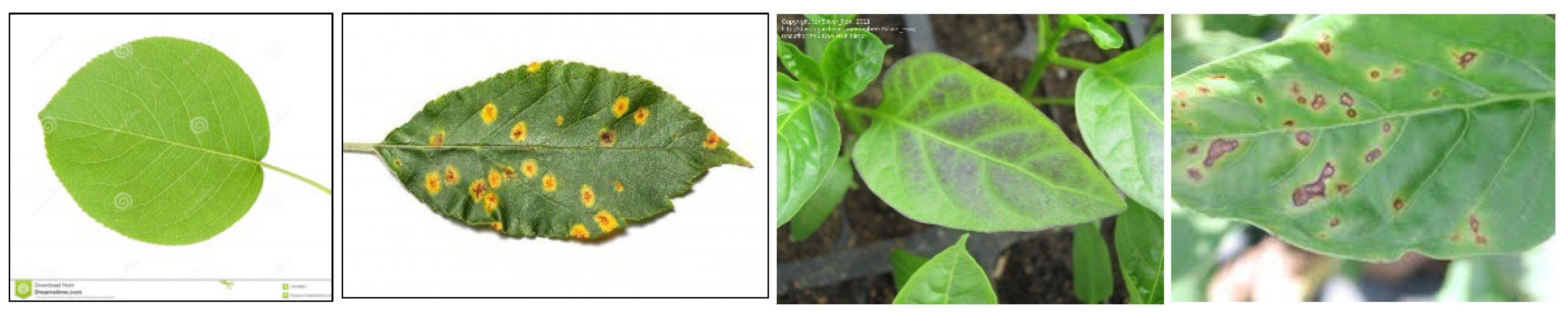
Example images of PlantDoc dataset used in our experiment. Left to right: images of apple leaf, apple leaf with rust disease, healthy bell pepper leaf, and bell pepper leaf with spot disease.
Figure 5.
Example images of PlantDoc dataset used in our experiment. Left to right: images of apple leaf, apple leaf with rust disease, healthy bell pepper leaf, and bell pepper leaf with spot disease.

Figure 6.
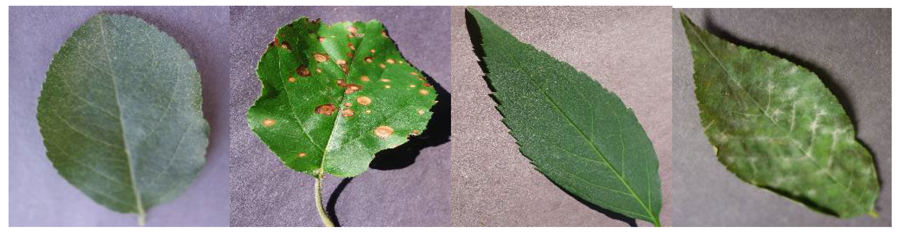
Example images of PlantVillage dataset used in our experiment. Left to right: images of healthy apple leaf, apple leaf with black rot disease, healthy cherry leaf, and cherry leaf with powdery mildew disease.
Figure 6.
Example images of PlantVillage dataset used in our experiment. Left to right: images of healthy apple leaf, apple leaf with black rot disease, healthy cherry leaf, and cherry leaf with powdery mildew disease.

Figure 7.
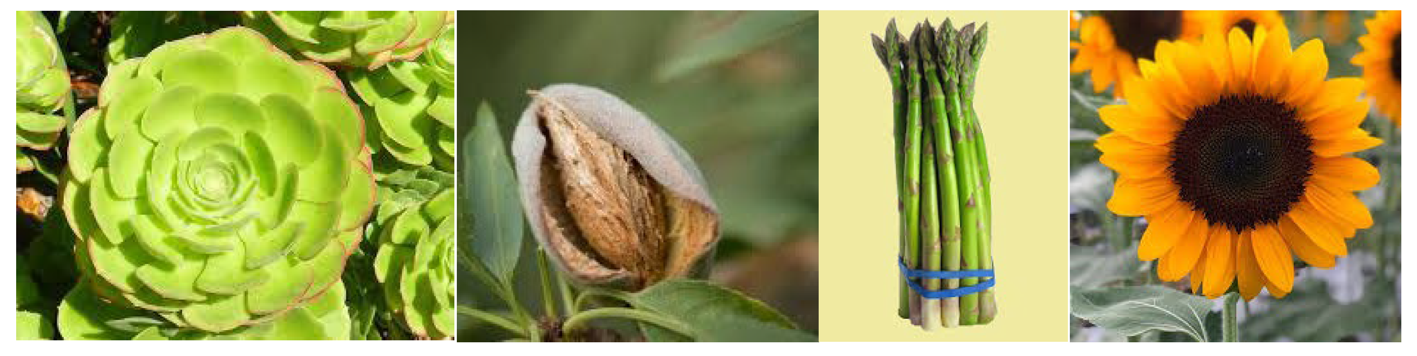
Example images of Plants dataset used in our experiment. Left to right: images of aeonium, almond, asparagus, and sunflower.
Figure 7.
Example images of Plants dataset used in our experiment. Left to right: images of aeonium, almond, asparagus, and sunflower.

Figure 8.
Training loss, validation loss, and validation accuracy curves of PI-GAN and PI-CNN with Fruits-360 dataset. (a,b) training loss and validation loss curves, respectively, of PI-GAN; (c,d) show the training and validation loss and accuracy curves of the proposed PI-CNN, respectively.
Figure 8.
Training loss, validation loss, and validation accuracy curves of PI-GAN and PI-CNN with Fruits-360 dataset. (a,b) training loss and validation loss curves, respectively, of PI-GAN; (c,d) show the training and validation loss and accuracy curves of the proposed PI-CNN, respectively.


Figure 9.
Examples of images augmented by conventional augmentation methods. Images augmented by (a) flipping and in-plane rotation; (b) image shifting in four directions; (c) the adjustments of brightness and contrast; (d) Gaussian blurring; (e) scaling.
Figure 9.
Examples of images augmented by conventional augmentation methods. Images augmented by (a) flipping and in-plane rotation; (b) image shifting in four directions; (c) the adjustments of brightness and contrast; (d) Gaussian blurring; (e) scaling.


Figure 10.
Examples of images augmented by PI-GAN. Left to right: (a) mango, date, and augmented image; (b) pear, mango, and augmented image; (c) huckleberry, date, and augmented image; (d) maracuja, tamarillo, and augmented image.
Figure 10.
Examples of images augmented by PI-GAN. Left to right: (a) mango, date, and augmented image; (b) pear, mango, and augmented image; (c) huckleberry, date, and augmented image; (d) maracuja, tamarillo, and augmented image.

Figure 11.
Comparison of F1-scores based on all the datasets (original dataset (O), reduced dataset (R), dataset augmented by conventional method (T), and dataset augmented by PI-GAN (G)). The datasets have been reduced to 70%.
Figure 11.
Comparison of F1-scores based on all the datasets (original dataset (O), reduced dataset (R), dataset augmented by conventional method (T), and dataset augmented by PI-GAN (G)). The datasets have been reduced to 70%.

Figure 12.
Comparison of F1-scores based on all the datasets (original dataset (O), reduced dataset (R), dataset augmented by conventional method (T), and dataset augmented by PI-GAN (G)). The datasets have been reduced to 50%.
Figure 12.
Comparison of F1-scores based on all the datasets (original dataset (O), reduced dataset (R), dataset augmented by conventional method (T), and dataset augmented by PI-GAN (G)). The datasets have been reduced to 50%.

Figure 13.
Comparison of F1-scores based on all the datasets (original dataset (O), reduced dataset (R), dataset augmented by conventional method (T), and dataset augmented by PI-GAN (G)). The datasets have been reduced to 30%.
Figure 13.
Comparison of F1-scores based on all the datasets (original dataset (O), reduced dataset (R), dataset augmented by conventional method (T), and dataset augmented by PI-GAN (G)). The datasets have been reduced to 30%.

Figure 14.
Comparison of F1-scores based on all the datasets (original dataset (O), reduced dataset (R), dataset augmented by conventional method (T), and dataset augmented by PI-GAN (G)). The datasets have been reduced to 10%.
Figure 14.
Comparison of F1-scores based on all the datasets (original dataset (O), reduced dataset (R), dataset augmented by conventional method (T), and dataset augmented by PI-GAN (G)). The datasets have been reduced to 10%.

Figure 15.
Error cases by the proposed PI-GAN. From the left to right: (a) date, carambula, and augmented date; (b) pineapple, cactus fruit, and augmented pineapple.
Figure 15.
Error cases by the proposed PI-GAN. From the left to right: (a) date, carambula, and augmented date; (b) pineapple, cactus fruit, and augmented pineapple.

Figure 16.
Error cases by the proposed PI-CNN. From the left to right: (a) apple, peach, and augmented apple; (b) peach, apple, and augmented peach.
Figure 16.
Error cases by the proposed PI-CNN. From the left to right: (a) apple, peach, and augmented apple; (b) peach, apple, and augmented peach.

Figure 17.
Training and validation loss curves. Curves obtained by using training sets with size of (a) 70%, (b) 50%, (c) 30%, (d) 10%. Curves obtained by using training sets augmented from training sets with size of (e) 70%, (f) 50%, (g) 30%, (h) 10%.
Figure 17.
Training and validation loss curves. Curves obtained by using training sets with size of (a) 70%, (b) 50%, (c) 30%, (d) 10%. Curves obtained by using training sets augmented from training sets with size of (e) 70%, (f) 50%, (g) 30%, (h) 10%.


Table 1.
Comparison between the proposed and previous methods for plant image classification.
| Methods | Advantages | Disadvantages | |
|---|---|---|---|
| Large training set-based | [1,2,3,4,5,6,7,8,9,10,11,12,13,14] | High accuracy | Does not consider small training sets |
| Small training set-based | Proposed method | Considers various sizes of training sets. Considers various sizes of training sets | Lower accuracy than that achieved when a large training set is used |
Table 2.
Description of the generator network used in our PI-GAN.
| Layer Number | Layer Type | Times | Number of Filters | Number of Parameters | Layer Connection (Connected to) |
|---|---|---|---|---|---|
| 0 | input_layer_1 | ×1 | 0 | 0 | input_1 |
| 1 | input_layer_2 | ×1 | 0 | 0 | input_2 |
| 2 | encoder_1 | ×4 | 128 | 605,696 | input_layer_1 |
| 3 | encoder_2 | ×4 | 128 | 605,696 | input_layer_2 |
| 4 | res_block_1 | ×2 | 128 | 590,592 | encoder_1 |
| 5 | res_block_2 | ×2 | 128 | 590,592 | encoder_2 |
| 6 | concat | ×1 | 0 | 0 | res_block_1 & res_block_2 |
| 7 | res_block_3 | ×3 | 256 | 885,888 | concat |
| 8 | decoder | ×4 | 128 | 1,328,640 | res_block_3 |
| 9 | conv2d (tanh) | ×1 | 3 | 3459 | decoder |
Total number of trainable parameters: 4,610,563.
Table 3.
Description of an encoder block of the generator network.
| Layer Number | Layer Type | Layer Connection (Connected to) |
|---|---|---|
| 1 | conv2d_1 | input |
| 2 | prelu_1 | conv2d_1 |
| 3 | conv2d_2 | prelu_1 |
| 4 | prelu_2 | conv2d_2 |
| 5 | max_pool | prelu_2 |
Table 4.
Description of a decoder block of the generator network.
| Layer Number | Layer Type | Layer Connection (Connected to) |
|---|---|---|
| 1 | conv2d_1 | input |
| 2 | prelu_1 | conv2d_1 |
| 3 | conv2d_2 | prelu_1 |
| 4 | prelu_2 | conv2d_2 |
| 5 | Up2 | prelu_2 |
Table 5.
Description of a residual block of the generator network.
| Layer Number | Layer Type | Layer Connection (Connected to) |
|---|---|---|
| 1 | conv2d_1 | input |
| 2 | prelu | conv2d_1 |
| 3 | conv2d_2 | prelu |
| 4 | add | conv2d_2 & input |
Table 6.
Description of the discriminator network of PI-GAN.
| Layer Number | Layer Type | Times | Number of Filters | Number of Strides | Number of Parameters | Layer Connection (Connected to) |
|---|---|---|---|---|---|---|
| 0 | input layer | ×1 | 0 | 0 | 0 | input |
| 1 | conv2d | ×1 | 128 | 1 | 3584 | input layer |
| 2 | lrelu_1 | ×1 | 0 | 0 | 0 | conv2d |
| 3 | disc_block | ×5 | 128, 128 256, 256, 256 | 1, 1 2, 2, 2 | 1,770,496 | lrelu_1 |
| 4 | lrelu_2 | ×1 | 0 | 0 | 0 | disc_block |
| 5 | FC (sigmoid) | ×1 | class# | 0 | 173,057 | lrelu_2 |
Total number of trainable parameters: 1,947,137.
Table 7.
Description of a convolution block of the discriminator network.
| Layer Number | Layer Type | Layer Connection (Connected to) |
|---|---|---|
| 1 | conv2d | input |
| 2 | lrelu | conv2d |
Table 8.
Description of the proposed PI-CNN.
| Layer Number | Layer Type | Number of Filters | Number of Parameters | Layer Connection (Connected to) |
|---|---|---|---|---|
| 1 | input layer_1 | 0 | 0 | input |
| 2 | conv2d_1 | 64 | 1792 | input layer_1 |
| 3 | conv2d_2 | 64 | 36,928 | conv2d_1 |
| 4 | max_pool_1 | 0 | 0 | conv2d_2 |
| 5 | res_block_1 | 64 | 73,920 | max_pool_1 |
| 6 | res_block_2 | 64 | 73,920 | res_block_1 |
| 7 | res_block_3 | 64 | 73,920 | res_block_2 |
| 8 | res_block_4 | 64 | 73,920 | res_block_3 |
| 9 | conv2d_3 | 128 | 73,856 | res_block_4 |
| 10 | conv2d_4 | 128 | 147,584 | conv2d_3 |
| 11 | max_pool_2 | 0 | 0 | conv2d_4 |
| 12 | res_block_5 | 128 | 295,296 | max_pool_2 |
| 13 | res_block_6 | 128 | 295,296 | res_block_5 |
| 14 | res_block_7 | 128 | 295,296 | res_block_6 |
| 15 | res_block_8 | 128 | 295,296 | res_block_7 |
| 16 | conv2d_5 | 128 | 147,584 | res_block_8 |
| 17 | conv2d_6 | 128 | 147,584 | conv2d_5 |
| 18 | max_pool_3 | 0 | 0 | conv2d_6 |
| 19 | res_block_9 | 128 | 295,296 | max_pool_3 |
| 20 | res_block_10 | 128 | 295,296 | res_block_9 |
| 21 | res_block_11 | 128 | 295,296 | res_block_10 |
| 22 | res_block_12 | 128 | 295,296 | res_block_11 |
| 23 | conv2d_7 | 128 | 147,584 | res_block_12 |
| 24 | conv2d_8 | 128 | 147,584 | conv2d_7 |
| 25 | max_pool_4 | 0 | 0 | conv2d_8 |
| 26 | res_block_13 | 128 | 295,296 | max_pool_4 |
| 27 | res_block_14 | 128 | 295,296 | res_block_13 |
| 28 | res_block_15 | 128 | 295,296 | res_block_14 |
| 29 | res_block_16 | 128 | 295,296 | res_block_15 |
| 30 | FC (softmax) | class# | 258,062 | res_block_16 |
Total number of trainable parameters: 4,947,790.
Table 9.
Summary of the datasets.
| Datasets | Training Sets | Test Sets | Validation Sets | Dimension | Depth | Extension | Class# |
|---|---|---|---|---|---|---|---|
| Fruits-360 | 41,322 | 12,877 | 1000 | 100 × 100 | 24 | jpg | 81 |
| PlantVillage | 40,000 | 13,305 | 1000 | 256 × 256 | 24 | jpg | 38 |
| PlantDoc | 2336 | 200 | 36 | 150 × 150–5616 × 3744 | 24 | jpg | 27 |
| Plants | 13,149 | 5218 | 1521 | 104 × 104–3168 × 4752 | 24 | jpg | 99 |
Table 10.
Detailed explanations of train and test sets used in our experiments.
| Datasets | Training Sets | Test Sets | Validation Sets | ||||
|---|---|---|---|---|---|---|---|
| 100% | 70% | 50% | 30% | 10% | |||
| Fruits-360 | 41,322 | 28,926 | 20,661 | 12,396 | 4132 | 12,877 | 1000 |
| PlantVillage | 40,000 | 28,000 | 20,000 | 12,000 | 4000 | 13,305 | 1000 |
| PlantDoc | 2336 | 1635 | 1168 | 700 | 233 | 200 | 36 |
| Plants | 13,149 | 9204 | 6574 | 3944 | 1314 | 5218 | 1521 |
Table 11.
Detailed explanations of train and test subsets used in our experiments. Training was performed by combining the training sets of the Plants and PlantDoc datasets (the numbers with ‘*’).
Table 11.
Detailed explanations of train and test subsets used in our experiments. Training was performed by combining the training sets of the Plants and PlantDoc datasets (the numbers with ‘*’).
| Datasets | Train Sets | Test Sets | Validation Sets | |||
|---|---|---|---|---|---|---|
| Crop | Disease | Crop | Disease | Crop | Disease | |
| Fruits-360 | 41,322 | 12,877 | 1000 | |||
| PlantVillage | 11,222 | 28,778 | 3592 | 9713 | 270 | 730 |
| PlantDoc | 757 * | 1579 * | 76 | 124 | 14 | 22 |
| Plants | 13,149 * | 5218 | 1521 | |||
Table 12.
Search space and selected values of hyperparameters for PI-GAN.
| Parameters | Weight Decay (Weight Regularization L2) | Loss | Kernel Initializer | Bias Initializer | Optimizer | Learning Rate | Beta_1 | Beta_2 | Epsilon | Epochs | Batch Size |
|---|---|---|---|---|---|---|---|---|---|---|---|
| Search Space | [0.001, 0.01, 0.1] | [“binary cross-entropy,” “VGG-19”] | “glorot uniform” | “zeros” | [“SGD,” “adam”] | [0.0001, 0.001, 0.01, 0.1] | [0.7, 0.8, 0.9] | [0.8, 0.9, 0.999] | [1 × 10⁻⁹, 1 × 10⁻⁸, 1 × 10⁻⁷] | [1–50] | [1, 4, 8, 16] |
| Selected Value | 0.01 | “binary cross-entropy” | “glorot uniform” | “zeros” | “adam” | 0.0001 | 0.9 | 0.999 | 1 × 10⁻⁸ | 50 | 8 |
Table 13.
Search space and selected values of hyperparameters for PI-CNN.
| Parameters | Learning Rate Decay (for SGD) | Momentum (for SGD) | Loss | Metrics | Optimizer | Learning Rate | Epochs | Batch Size |
|---|---|---|---|---|---|---|---|---|
| Search Space | [0.000001, 0.00001, 0.0001] | [0.9, 0.8, 0.7] | “categorical cross-entropy” | [“categorical_accuracy”, “accuracy”] | [“SGD,” “adam”] | [0.0001, 0.001, 0.01, 0.1] | [1–40] | [1, 4, 8, 16] |
| Selected Value | 0.00001 | 0.9 | “categorical cross-entropy” | ” accuracy” | “adam” | 0.0001 | 30 | 8 |
Table 14.
Comparison of accuracies by the proposed PI-GAN generator and variants of generators in the Fruits-360 training set of 50%.
Table 14.
Comparison of accuracies by the proposed PI-GAN generator and variants of generators in the Fruits-360 training set of 50%.
| Methods | TPR | PPV | ACC | F1-Score |
|---|---|---|---|---|
| encoder-decoder ×1 | 76.00 | 80.29 | 86.74 | 78.08 |
| encoder-decoder ×2 | 76.43 | 81.62 | 86.07 | 78.94 |
| encoder-decoder ×3 | 76.56 | 80.40 | 87.49 | 78.43 |
| encoder-decoder ×4 (proposed) | 76.70 | 81.65 | 87.94 | 79.18 |
| encoder-decoder ×5 | 75.85 | 81.12 | 86.62 | 78.40 |
Table 15.
Comparison of accuracies by the proposed PI-CNN and variants of CNN in the Fruits-360 dataset.
Table 15.
Comparison of accuracies by the proposed PI-CNN and variants of CNN in the Fruits-360 dataset.
| Methods | TPR | PPV | ACC | F1-Score |
|---|---|---|---|---|
| res_block-14 | 95.01 | 93.15 | 97.38 | 94.07 |
| res _block-15 | 95.24 | 92.43 | 98.53 | 93.81 |
| res _block-16 (proposed) | 95.40 | 94.33 | 98.59 | 94.87 |
| res _block-17 | 95.14 | 92.46 | 96.94 | 93.78 |
Table 16.
Comparison of accuracies achieved by the proposed PI-CNN in the original and reduced datasets. The accuracies were achieved in the PlantVillage dataset (unit: %).
Table 16.
Comparison of accuracies achieved by the proposed PI-CNN in the original and reduced datasets. The accuracies were achieved in the PlantVillage dataset (unit: %).
| Dataset | Disease | Crop | |||||||
|---|---|---|---|---|---|---|---|---|---|
| TPR | PPV | ACC | F1-Score | TPR | PPV | ACC | F1-Score | ||
| Original | 100% | 89.62 | 95.13 | 97.26 | 92.38 | 98.48 | 94.76 | 99.57 | 96.62 |
| Reduced | 70% | 86.20 | 89.11 | 92.34 | 87.66 | 89.10 | 86.27 | 90.41 | 87.69 |
| 50% | 71.89 | 78.67 | 84.70 | 75.28 | 71.10 | 78.60 | 84.64 | 74.85 | |
| 30% | 52.80 | 47.48 | 65.54 | 50.14 | 53.20 | 45.87 | 63.13 | 49.54 | |
| 10% | 31.84 | 34.29 | 43.55 | 33.07 | 32.98 | 33.25 | 43.91 | 33.12 | |
Table 17.
Comparison of accuracies achieved by the proposed PI-CNN in the original and reduced datasets. The accuracies were achieved in the PlantDoc dataset (unit: %).
Table 17.
Comparison of accuracies achieved by the proposed PI-CNN in the original and reduced datasets. The accuracies were achieved in the PlantDoc dataset (unit: %).
| Dataset | Disease | Crop | |||||||
|---|---|---|---|---|---|---|---|---|---|
| TPR | PPV | ACC | F1-Score | TPR | PPV | ACC | F1-Score | ||
| Original | 100% | 66.13 | 67.87 | 80.36 | 67.00 | 78.26 | 74.66 | 86.57 | 76.46 |
| Reduced | 70% | 59.54 | 54.48 | 74.08 | 57.01 | 70.37 | 64.78 | 80.81 | 67.58 |
| 50% | 40.20 | 39.21 | 61.05 | 39.71 | 51.95 | 48.15 | 72.55 | 50.05 | |
| 30% | 36.62 | 29.31 | 45.21 | 32.97 | 41.62 | 35.31 | 53.14 | 38.47 | |
| 10% | 21.30 | 22.51 | 29.12 | 21.91 | 21.98 | 22.41 | 32.18 | 22.20 | |
Table 18.
Comparison of accuracies achieved by the proposed PI-CNN in the original and reduced datasets. The accuracies were achieved in the Plants and Fruits-360 dataset (unit: %).
Table 18.
Comparison of accuracies achieved by the proposed PI-CNN in the original and reduced datasets. The accuracies were achieved in the Plants and Fruits-360 dataset (unit: %).
| Dataset | Plants Dataset | Fruits-360 Dataset | |||||||
|---|---|---|---|---|---|---|---|---|---|
| TPR | PPV | ACC | F1-Score | TPR | PPV | ACC | F1-Score | ||
| Original | 100% | 90.10 | 86.11 | 96.52 | 88.11 | 95.40 | 94.33 | 98.59 | 94.87 |
| Reduced | 70% | 80.46 | 76.40 | 92.81 | 78.43 | 91.70 | 89.00 | 91.80 | 90.35 |
| 50% | 62.71 | 60.22 | 84.10 | 61.47 | 72.47 | 78.63 | 83.63 | 75.55 | |
| 30% | 49.74 | 41.50 | 60.34 | 45.62 | 52.68 | 45.86 | 65.44 | 49.27 | |
| 10% | 30.66 | 31.33 | 40.85 | 31.00 | 39.37 | 36.19 | 48.31 | 37.78 | |
Table 19.
Comparison of accuracies achieved by the proposed PI-CNN in the original and augmented datasets. The accuracies were achieved in the PlantVillage dataset (unit: %).
Table 19.
Comparison of accuracies achieved by the proposed PI-CNN in the original and augmented datasets. The accuracies were achieved in the PlantVillage dataset (unit: %).
| Dataset | Disease | Crop | |||||||
|---|---|---|---|---|---|---|---|---|---|
| Before Augmentation | After Augmentation | TPR | PPV | ACC | F1-Score | TPR | PPV | ACC | F1-Score |
| 100% | 100% | 89.62 | 95.13 | 97.26 | 92.38 | 98.48 | 94.76 | 99.57 | 96.62 |
| 70% | 100% | 86.89 | 90.17 | 93.87 | 88.53 | 89.76 | 88.96 | 92.60 | 89.36 |
| 50% | 100% | 71.66 | 79.88 | 86.97 | 75.77 | 73.58 | 80.84 | 84.82 | 77.21 |
| 30% | 100% | 54.86 | 49.34 | 66.13 | 52.10 | 53.11 | 46.95 | 63.34 | 50.03 |
| 10% | 100% | 32.71 | 36.21 | 44.28 | 34.46 | 32.80 | 34.97 | 45.29 | 33.89 |
Table 20.
Comparison of accuracies achieved by the proposed PI-CNN in the original and augmented datasets. The accuracies were achieved in the PlantDoc dataset (unit: %).
Table 20.
Comparison of accuracies achieved by the proposed PI-CNN in the original and augmented datasets. The accuracies were achieved in the PlantDoc dataset (unit: %).
| Dataset | Disease | Crop | |||||||
|---|---|---|---|---|---|---|---|---|---|
| Before Augmentation | After Augmentation | TPR | PPV | ACC | F1-Score | TPR | PPV | ACC | F1-Score |
| 100% | 100% | 66.13 | 67.87 | 80.36 | 67.00 | 78.26 | 74.66 | 86.57 | 76.46 |
| 70% | 100% | 60.12 | 56.23 | 76.82 | 58.18 | 71.86 | 65.80 | 82.40 | 68.83 |
| 50% | 100% | 42.83 | 39.55 | 62.69 | 41.19 | 53.36 | 50.92 | 72.31 | 52.14 |
| 30% | 100% | 38.87 | 33.71 | 48.8 | 36.29 | 44.53 | 38.2 | 58.57 | 42.87 |
| 10% | 100% | 23.40 | 22.88 | 30.30 | 23.14 | 24.45 | 23.80 | 34.69 | 24.13 |
Table 21.
Comparison of accuracies achieved by the proposed PI-CNN in the original and augmented datasets. The accuracies were achieved in the Plants and Fruits-360 dataset (unit: %).
Table 21.
Comparison of accuracies achieved by the proposed PI-CNN in the original and augmented datasets. The accuracies were achieved in the Plants and Fruits-360 dataset (unit: %).
| Dataset | Plants Dataset | Fruits-360 Dataset | |||||||
|---|---|---|---|---|---|---|---|---|---|
| Before Augmentation | After Augmentation | TPR | PPV | ACC | F1-Score | TPR | PPV | ACC | F1-Score |
| 100% | 100% | 90.10 | 86.11 | 96.52 | 88.11 | 95.40 | 94.33 | 98.59 | 94.87 |
| 70% | 100% | 82.19 | 76.30 | 92.86 | 79.25 | 92.30 | 90.72 | 93.61 | 91.51 |
| 50% | 100% | 63.32 | 61.94 | 85.93 | 62.63 | 73.40 | 78.80 | 83.66 | 76.10 |
| 30% | 100% | 51.52 | 41.30 | 62.47 | 46.41 | 54.39 | 47.25 | 67.50 | 50.82 |
| 10% | 100% | 30.78 | 33.60 | 41.16 | 32.19 | 39.57 | 37.26 | 48.33 | 38.42 |
Table 22.
Comparison of accuracies achieved by the proposed PI-CNN in the original and augmented datasets. The accuracies were achieved in the PlantVillage dataset (unit: %).
Table 22.
Comparison of accuracies achieved by the proposed PI-CNN in the original and augmented datasets. The accuracies were achieved in the PlantVillage dataset (unit: %).
| Dataset | Disease | Crop | |||||||
|---|---|---|---|---|---|---|---|---|---|
| Before Augmentation | After Augmentation | TPR | PPV | ACC | F1-Score | TPR | PPV | ACC | F1-Score |
| 100% | 100% | 89.62 | 95.13 | 97.26 | 92.38 | 98.48 | 94.76 | 99.57 | 96.62 |
| 70% | 100% | 86.39 | 88.45 | 93.39 | 87.41 | 88.45 | 88.84 | 91.72 | 88.65 |
| 50% | 100% | 70.99 | 79.18 | 85.67 | 74.86 | 72.90 | 80.09 | 84.58 | 76.32 |
| 30% | 100% | 53.07 | 48.49 | 64.36 | 50.68 | 52.65 | 46.08 | 61.52 | 49.15 |
| 10% | 100% | 31.53 | 36.06 | 43.30 | 33.64 | 30.85 | 34.91 | 44.97 | 32.75 |
Table 23.
Comparison of accuracies achieved by the proposed PI-CNN in the original and augmented datasets. The accuracies were achieved in the PlantDoc dataset (unit: %).
Table 23.
Comparison of accuracies achieved by the proposed PI-CNN in the original and augmented datasets. The accuracies were achieved in the PlantDoc dataset (unit: %).
| Dataset | Disease | Crop | |||||||
|---|---|---|---|---|---|---|---|---|---|
| Before Augmentation | After Augmentation | TPR | PPV | ACC | F1-Score | TPR | PPV | ACC | F1-Score |
| 100% | 100% | 66.13 | 67.87 | 80.36 | 67.00 | 78.26 | 74.66 | 86.57 | 76.46 |
| 70% | 100% | 59.60 | 55.72 | 76.40 | 57.59 | 70.63 | 64.46 | 80.96 | 67.40 |
| 50% | 100% | 41.68 | 38.87 | 60.74 | 40.22 | 53.23 | 50.59 | 71.11 | 51.88 |
| 30% | 100% | 37.30 | 33.55 | 47.83 | 35.33 | 43.47 | 38.00 | 57.32 | 40.55 |
| 10% | 100% | 22.04 | 22.18 | 30.13 | 22.11 | 23.12 | 22.27 | 33.92 | 22.69 |
Table 24.
Comparison of accuracies achieved by the proposed PI-CNN in the original and augmented datasets. The accuracies were achieved in the Plants and Fruits-360 dataset (unit: %).
Table 24.
Comparison of accuracies achieved by the proposed PI-CNN in the original and augmented datasets. The accuracies were achieved in the Plants and Fruits-360 dataset (unit: %).
| Dataset | Plants dataset | Fruits-360 dataset | |||||||
|---|---|---|---|---|---|---|---|---|---|
| Before Augmentation | After Augmentation | TPR | PPV | ACC | F1-Score | TPR | PPV | ACC | F1-Score |
| 100% | 100% | 90.10 | 86.11 | 96.52 | 88.11 | 95.40 | 94.33 | 98.59 | 94.87 |
| 70% | 100% | 80.56 | 76.22 | 91.83 | 78.33 | 91.47 | 90.62 | 92.37 | 91.04 |
| 50% | 100% | 61.37 | 61.07 | 84.32 | 61.22 | 73.14 | 78.61 | 82.78 | 75.78 |
| 30% | 100% | 50.41 | 41.27 | 61.09 | 45.38 | 52.43 | 45.44 | 65.83 | 48.68 |
| 10% | 100% | 29.18 | 33.11 | 40.93 | 31.02 | 37.95 | 35.84 | 48.22 | 36.87 |
Table 25.
Comparison of accuracies achieved by the proposed PI-CNN in the original and PI-GAN-augmented datasets. The accuracies were achieved in the PlantVillage dataset (unit: %).
Table 25.
Comparison of accuracies achieved by the proposed PI-CNN in the original and PI-GAN-augmented datasets. The accuracies were achieved in the PlantVillage dataset (unit: %).
| Dataset Division | Disease | Crop | |||||||
|---|---|---|---|---|---|---|---|---|---|
| Before Augmentation | After Augmentation | TPR | PPV | ACC | F1-Score | TPR | PPV | ACC | F1-Score |
| 100% | 100% | 89.62 | 95.13 | 97.26 | 92.38 | 98.48 | 94.76 | 99.57 | 96.62 |
| 70% | 100% | 88.66 | 93.36 | 96.40 | 91.01 | 93.61 | 90.92 | 93.65 | 92.27 |
| 50% | 100% | 74.50 | 81.23 | 87.67 | 77.87 | 74.30 | 82.49 | 88.10 | 78.40 |
| 30% | 100% | 56.00 | 51.36 | 68.33 | 53.68 | 56.15 | 48.46 | 66.62 | 52.31 |
| 10% | 100% | 34.34 | 38.60 | 47.59 | 36.47 | 36.81 | 36.20 | 46.45 | 36.51 |
Table 26.
Comparison of accuracies achieved by the proposed PI-CNN in the original and PI-GAN-augmented datasets. The accuracies were achieved in the PlantDoc dataset (unit: %).
Table 26.
Comparison of accuracies achieved by the proposed PI-CNN in the original and PI-GAN-augmented datasets. The accuracies were achieved in the PlantDoc dataset (unit: %).
| Dataset Division | Disease | Crop | |||||||
|---|---|---|---|---|---|---|---|---|---|
| Before Augmentation | After Augmentation | TPR | PPV | ACC | F1-Score | TPR | PPV | ACC | F1-Score |
| 100% | 100% | 66.13 | 67.87 | 80.36 | 67.00 | 78.26 | 74.66 | 86.57 | 76.46 |
| 70% | 100% | 63.68 | 57.10 | 78.50 | 60.39 | 73.16 | 68.17 | 83.62 | 70.67 |
| 50% | 100% | 43.69 | 43.68 | 65.41 | 43.69 | 55.47 | 52.92 | 76.59 | 54.20 |
| 30% | 100% | 41.15 | 36.24 | 50.4 | 38.51 | 47.73 | 42.3 | 62.28 | 45.57 |
| 10% | 100% | 26.48 | 25.87 | 32.14 | 26.18 | 28.80 | 26.91 | 36.33 | 27.86 |
Table 27.
Comparison of accuracies achieved by the proposed PI-CNN in the original and PI-GAN-augmented datasets. The accuracies were achieved in the Plants and Fruits-360 datasets (unit: %).
Table 27.
Comparison of accuracies achieved by the proposed PI-CNN in the original and PI-GAN-augmented datasets. The accuracies were achieved in the Plants and Fruits-360 datasets (unit: %).
| Dataset Division | Plants | Fruits-360 | |||||||
|---|---|---|---|---|---|---|---|---|---|
| Before Augmentation | After Augmentation | TPR | PPV | ACC | F1-Score | TPR | PPV | ACC | F1-Score |
| 100% | 100% | 90.10 | 86.11 | 96.52 | 88.11 | 95.40 | 94.33 | 98.59 | 94.87 |
| 70% | 100% | 84.52 | 80.66 | 96.18 | 82.59 | 94.53 | 92.31 | 94.48 | 93.42 |
| 50% | 100% | 66.64 | 64.53 | 88.52 | 65.59 | 76.70 | 81.65 | 87.94 | 79.18 |
| 30% | 100% | 53.28 | 45.34 | 63.93 | 49.31 | 55.12 | 49.62 | 69.89 | 52.37 |
| 10% | 100% | 34.52 | 35.96 | 44.31 | 35.24 | 43.40 | 39.70 | 51.90 | 41.55 |
Table 28.
Comparison of accuracies achieved by the proposed PI-CNN in the original and PI-GAN-augmented datasets. The accuracies were achieved in the PlantVillage dataset (unit: %).
Table 28.
Comparison of accuracies achieved by the proposed PI-CNN in the original and PI-GAN-augmented datasets. The accuracies were achieved in the PlantVillage dataset (unit: %).
| Dataset Division | Disease | Crop | |||||||
|---|---|---|---|---|---|---|---|---|---|
| Before Augmentation | After Augmentation | TPR | PPV | ACC | F1-Score | TPR | PPV | ACC | F1-Score |
| 100% | 100% | 89.62 | 95.13 | 97.26 | 92.38 | 98.48 | 94.76 | 99.57 | 96.62 |
| 70% | 100% | 87.34 | 92.10 | 95.29 | 89.66 | 92.43 | 90.85 | 92.64 | 91.63 |
| 50% | 100% | 73.26 | 80.76 | 86.81 | 76.83 | 73.98 | 82.28 | 87.92 | 77.91 |
| 30% | 100% | 55.32 | 50.13 | 68.27 | 52.60 | 55.74 | 47.68 | 65.46 | 51.40 |
| 10% | 100% | 33.88 | 38.60 | 46.43 | 36.09 | 36.39 | 35.92 | 45.56 | 36.15 |
Table 29.
Comparison of accuracies achieved by the proposed PI-CNN in the original and PI-GAN-augmented datasets. The accuracies were achieved in the PlantDoc dataset (unit: %).
Table 29.
Comparison of accuracies achieved by the proposed PI-CNN in the original and PI-GAN-augmented datasets. The accuracies were achieved in the PlantDoc dataset (unit: %).
| Dataset Division | Disease | Crop | |||||||
|---|---|---|---|---|---|---|---|---|---|
| Before Augmentation | After Augmentation | TPR | PPV | ACC | F1-Score | TPR | PPV | ACC | F1-Score |
| 100% | 100% | 66.13 | 67.87 | 80.36 | 67.00 | 78.26 | 74.66 | 86.57 | 76.46 |
| 70% | 100% | 63.01 | 56.75 | 77.21 | 59.72 | 71.73 | 67.41 | 82.24 | 69.51 |
| 50% | 100% | 42.81 | 43.29 | 64.13 | 43.04 | 54.17 | 52.91 | 75.22 | 53.53 |
| 30% | 100% | 39.65 | 35.34 | 49.41 | 37.37 | 47.15 | 41.82 | 60.82 | 44.33 |
| 10% | 100% | 26.27 | 24.39 | 31.81 | 25.29 | 27.98 | 25.98 | 35.81 | 26.95 |
Table 30.
Comparison of accuracies achieved by the proposed PI-CNN in the original and PI-GAN-augmented datasets. The accuracies were achieved in the Plants and Fruits-360 datasets (unit: %).
Table 30.
Comparison of accuracies achieved by the proposed PI-CNN in the original and PI-GAN-augmented datasets. The accuracies were achieved in the Plants and Fruits-360 datasets (unit: %).
| Dataset Division | Plants | Fruits-360 | |||||||
|---|---|---|---|---|---|---|---|---|---|
| Before Augmentation | After Augmentation | TPR | PPV | ACC | F1-Score | TPR | PPV | ACC | F1-Score |
| 100% | 100% | 90.10 | 86.11 | 96.52 | 88.11 | 95.40 | 94.33 | 98.59 | 94.87 |
| 70% | 100% | 83.79 | 79.59 | 94.90 | 81.63 | 93.90 | 92.29 | 94.12 | 93.09 |
| 50% | 100% | 65.91 | 63.23 | 87.72 | 64.55 | 75.42 | 81.29 | 87.26 | 78.25 |
| 30% | 100% | 52.79 | 45.00 | 63.73 | 48.58 | 54.53 | 49.08 | 69.36 | 51.66 |
| 10% | 100% | 33.55 | 35.12 | 43.36 | 34.32 | 43.15 | 38.70 | 50.53 | 40.80 |
Table 31.
Comparison of accuracies achieved by the proposed PI-CNN and the existing methods in the original and reduced datasets. The accuracies were achieved in the PlantVillage dataset (unit: %).
Table 31.
Comparison of accuracies achieved by the proposed PI-CNN and the existing methods in the original and reduced datasets. The accuracies were achieved in the PlantVillage dataset (unit: %).
| Methods | Dataset | Disease | Crop | ||||||
|---|---|---|---|---|---|---|---|---|---|
| TPR | PPV | ACC | F1-Score | TPR | PPV | ACC | F1-Score | ||
| Wang [14] | 100% | 88.31 | 94.02 | 96.34 | 91.17 | 97.15 | 93.54 | 98.35 | 95.35 |
| 70% | 85.65 | 88.84 | 91.48 | 87.25 | 88.84 | 85.74 | 89.98 | 87.29 | |
| 50% | 70.85 | 77.64 | 84.04 | 74.25 | 70.58 | 77.51 | 83.24 | 74.05 | |
| 30% | 51.56 | 46.33 | 64.92 | 48.95 | 52.84 | 44.17 | 63.84 | 48.51 | |
| 10% | 30.54 | 33.89 | 43.12 | 32.22 | 32.01 | 32.98 | 43.54 | 32.50 | |
| Shahi [1] | 100% | 89.32 | 94.53 | 96.94 | 91.93 | 97.93 | 94.32 | 98.12 | 96.13 |
| 70% | 85.84 | 88.17 | 91.74 | 87.01 | 88.17 | 83.44 | 89.24 | 85.81 | |
| 50% | 69.45 | 76.17 | 82.61 | 72.81 | 70.82 | 76.32 | 82.42 | 73.57 | |
| 30% | 51.52 | 46.44 | 63.14 | 48.98 | 51.43 | 43.66 | 62.45 | 47.55 | |
| 10% | 29.14 | 33.48 | 42.78 | 31.31 | 31.52 | 32.74 | 42.49 | 32.13 | |
| Srivastava [5] | 100% | 88.90 | 94.86 | 97.10 | 91.79 | 97.73 | 94.51 | 98.40 | 96.10 |
| 70% | 84.90 | 88.25 | 91.12 | 86.55 | 89.00 | 85.35 | 88.92 | 87.14 | |
| 50% | 70.86 | 77.80 | 83.69 | 74.17 | 69.66 | 77.58 | 84.14 | 73.40 | |
| 30% | 52.30 | 46.91 | 65.13 | 49.46 | 52.35 | 45.69 | 63.13 | 48.80 | |
| 10% | 31.08 | 33.02 | 43.37 | 32.02 | 31.52 | 32.24 | 42.66 | 31.88 | |
| Jordan [46] | 100% | 88.20 | 94.12 | 96.91 | 91.06 | 97.10 | 93.85 | 98.62 | 95.45 |
| 70% | 86.06 | 89.01 | 91.37 | 87.51 | 89.01 | 85.48 | 90.05 | 87.21 | |
| 50% | 71.39 | 78.65 | 84.35 | 74.85 | 70.01 | 78.36 | 84.58 | 73.95 | |
| 30% | 52.07 | 47.11 | 65.20 | 49.46 | 52.12 | 45.25 | 62.67 | 48.44 | |
| 10% | 31.38 | 33.70 | 42.53 | 32.50 | 32.96 | 32.79 | 42.93 | 32.87 | |
| Ours | 100% | 89.62 | 95.13 | 97.26 | 92.38 | 98.48 | 94.76 | 99.57 | 96.62 |
| 70% | 86.20 | 89.11 | 92.34 | 87.66 | 89.10 | 86.27 | 90.41 | 87.69 | |
| 50% | 71.89 | 78.67 | 84.70 | 75.28 | 71.10 | 78.60 | 84.64 | 74.85 | |
| 30% | 52.80 | 47.48 | 65.54 | 50.14 | 53.20 | 45.87 | 63.13 | 49.54 | |
| 10% | 31.84 | 34.29 | 43.55 | 33.07 | 32.98 | 33.25 | 43.91 | 33.12 | |
Table 32.
Comparison of accuracies achieved by the proposed PI-CNN and the existing methods in the original and reduced datasets. The accuracies were achieved in the PlantDoc dataset (unit: %).
Table 32.
Comparison of accuracies achieved by the proposed PI-CNN and the existing methods in the original and reduced datasets. The accuracies were achieved in the PlantDoc dataset (unit: %).
| Methods | Dataset | Disease | Crop | ||||||
|---|---|---|---|---|---|---|---|---|---|
| TPR | PPV | ACC | F1-Score | TPR | PPV | ACC | F1-Score | ||
| Wang [14] | 100% | 65.12 | 66.49 | 79.82 | 65.81 | 77.37 | 73.54 | 84.95 | 75.46 |
| 70% | 58.26 | 54.39 | 73.07 | 56.33 | 68.50 | 64.74 | 79.89 | 66.62 | |
| 50% | 38.30 | 38.20 | 60.67 | 38.25 | 51.25 | 47.82 | 71.31 | 49.54 | |
| 30% | 35.85 | 28.38 | 44.18 | 32.12 | 40.17 | 34.88 | 52.69 | 37.53 | |
| 10% | 19.42 | 21.31 | 27.68 | 20.37 | 20.26 | 21.29 | 30.21 | 20.78 | |
| Shahi [1] | 100% | 64.58 | 66.66 | 78.83 | 65.62 | 77.79 | 73.42 | 86.02 | 75.61 |
| 70% | 58.90 | 53.72 | 72.76 | 56.31 | 68.85 | 63.69 | 80.42 | 66.27 | |
| 50% | 38.79 | 38.64 | 59.73 | 38.72 | 50.41 | 47.96 | 71.07 | 49.19 | |
| 30% | 35.79 | 28.59 | 44.50 | 32.19 | 39.76 | 34.05 | 51.50 | 36.91 | |
| 10% | 21.03 | 22.06 | 28.33 | 21.55 | 21.58 | 21.01 | 31.35 | 21.30 | |
| Srivastava [5] | 100% | 65.66 | 67.43 | 79.03 | 66.53 | 77.25 | 74.00 | 85.97 | 75.59 |
| 70% | 58.55 | 53.13 | 73.70 | 55.71 | 69.11 | 64.49 | 79.72 | 66.72 | |
| 50% | 39.90 | 38.93 | 60.88 | 39.41 | 50.83 | 47.19 | 72.07 | 48.95 | |
| 30% | 36.11 | 29.00 | 44.13 | 32.17 | 40.40 | 34.81 | 52.33 | 37.40 | |
| 10% | 19.99 | 21.04 | 27.69 | 20.50 | 20.76 | 21.71 | 31.72 | 21.22 | |
| Jordan [46] | 100% | 65.12 | 67.64 | 79.78 | 66.36 | 76.78 | 74.64 | 86.28 | 75.69 |
| 70% | 58.16 | 53.72 | 72.98 | 55.85 | 70.33 | 64.06 | 80.59 | 67.05 | |
| 50% | 39.56 | 37.77 | 60.27 | 38.64 | 50.92 | 46.96 | 72.37 | 48.86 | |
| 30% | 35.60 | 28.92 | 43.78 | 31.91 | 40.23 | 33.95 | 51.92 | 36.83 | |
| 10% | 19.92 | 21.46 | 27.93 | 20.66 | 20.59 | 21.26 | 31.63 | 20.92 | |
| Ours | 100% | 66.13 | 67.87 | 80.36 | 67.00 | 78.26 | 74.66 | 86.57 | 76.46 |
| 70% | 59.54 | 54.48 | 74.08 | 57.01 | 70.37 | 64.78 | 80.81 | 67.58 | |
| 50% | 40.20 | 39.21 | 61.05 | 39.71 | 51.95 | 48.15 | 72.55 | 50.05 | |
| 30% | 36.62 | 29.31 | 45.21 | 32.97 | 41.62 | 35.31 | 53.14 | 38.47 | |
| 10% | 21.30 | 22.51 | 29.12 | 21.91 | 21.98 | 22.41 | 32.18 | 22.20 | |
Table 33.
Comparison of accuracies achieved by the proposed PI-CNN and the existing methods in the original and reduced datasets. The accuracies were achieved in the Plants and Fruits-360 datasets (unit: %).
Table 33.
Comparison of accuracies achieved by the proposed PI-CNN and the existing methods in the original and reduced datasets. The accuracies were achieved in the Plants and Fruits-360 datasets (unit: %).
| Methods | Dataset | Plants | Fruits-360 | ||||||
|---|---|---|---|---|---|---|---|---|---|
| TPR | PPV | ACC | F1-Score | TPR | PPV | ACC | F1-Score | ||
| Wang [14] | 100% | 89.72 | 85.29 | 95.63 | 87.51 | 94.47 | 94.04 | 97.88 | 94.26 |
| 70% | 80.25 | 76.35 | 92.23 | 78.30 | 91.24 | 88.77 | 90.87 | 90.01 | |
| 50% | 62.55 | 59.85 | 84.10 | 61.20 | 72.24 | 78.49 | 82.93 | 75.37 | |
| 30% | 48.89 | 40.71 | 59.51 | 44.80 | 52.06 | 45.20 | 65.16 | 48.63 | |
| 10% | 29.68 | 30.60 | 40.61 | 30.14 | 38.84 | 35.24 | 47.54 | 37.04 | |
| Shahi [1] | 100% | 89.35 | 84.47 | 94.75 | 86.91 | 93.53 | 93.74 | 97.17 | 93.64 |
| 70% | 80.04 | 76.30 | 91.66 | 78.17 | 90.77 | 88.54 | 89.94 | 89.66 | |
| 50% | 62.39 | 59.48 | 84.09 | 60.94 | 72.01 | 78.35 | 82.23 | 75.18 | |
| 30% | 48.03 | 39.93 | 58.67 | 43.98 | 51.45 | 44.55 | 64.88 | 48.00 | |
| 10% | 28.70 | 29.86 | 40.37 | 29.28 | 38.32 | 34.30 | 46.77 | 36.31 | |
| Srivastava [5] | 100% | 89.74 | 85.96 | 95.60 | 87.81 | 94.26 | 93.10 | 98.25 | 93.68 |
| 70% | 79.98 | 75.47 | 92.57 | 77.66 | 90.91 | 88.15 | 90.60 | 89.51 | |
| 50% | 61.43 | 59.79 | 82.97 | 60.60 | 72.40 | 77.95 | 82.62 | 75.07 | |
| 30% | 49.53 | 40.93 | 58.93 | 44.82 | 51.60 | 45.84 | 64.34 | 48.55 | |
| 10% | 30.00 | 31.06 | 40.28 | 30.52 | 38.95 | 35.71 | 48.00 | 37.26 | |
| Jordan [46] | 100% | 89.34 | 85.20 | 95.71 | 87.22 | 94.22 | 93.88 | 97.43 | 94.05 |
| 70% | 79.53 | 75.59 | 92.58 | 77.51 | 91.61 | 88.34 | 90.54 | 89.95 | |
| 50% | 61.84 | 58.88 | 82.77 | 60.33 | 72.30 | 78.34 | 83.10 | 75.20 | |
| 30% | 49.30 | 40.41 | 60.03 | 44.41 | 52.08 | 45.12 | 65.00 | 48.35 | |
| 10% | 30.24 | 30.34 | 40.50 | 30.29 | 39.37 | 35.31 | 48.11 | 37.23 | |
| Ours | 100% | 90.10 | 86.11 | 96.52 | 88.11 | 95.40 | 94.33 | 98.59 | 94.87 |
| 70% | 80.46 | 76.40 | 92.81 | 78.43 | 91.70 | 89.00 | 91.80 | 90.35 | |
| 50% | 62.71 | 60.22 | 84.10 | 61.47 | 72.47 | 78.63 | 83.63 | 75.55 | |
| 30% | 49.74 | 41.50 | 60.34 | 45.62 | 52.68 | 45.86 | 65.44 | 49.27 | |
| 10% | 30.66 | 31.33 | 40.85 | 31.00 | 39.37 | 36.19 | 48.31 | 37.78 | |
Table 34.
Processing time of the methods per image (unit: ms).
| Methods | Processing Time |
|---|---|
| Image augmentation by PI-GAN | 45.92 |
| Classification by PI-CNN | 51.85 |
| Total | 97.77 |
Publisher’s Note: MDPI stays neutral with regard to jurisdictional claims in published maps and institutional affiliations. |
© 2022 by the authors. Licensee MDPI, Basel, Switzerland. This article is an open access article distributed under the terms and conditions of the Creative Commons Attribution (CC BY) license (https://creativecommons.org/licenses/by/4.0/).
Share and Cite
MDPI and ACS Style
Batchuluun, G.; Nam, S.H.; Park, K.R. Deep Learning-Based Plant-Image Classification Using a Small Training Dataset. Mathematics 2022, 10, 3091. https://0-doi-org.brum.beds.ac.uk/10.3390/math10173091
AMA Style
Batchuluun G, Nam SH, Park KR. Deep Learning-Based Plant-Image Classification Using a Small Training Dataset. Mathematics. 2022; 10(17):3091. https://0-doi-org.brum.beds.ac.uk/10.3390/math10173091
Chicago/Turabian StyleBatchuluun, Ganbayar, Se Hyun Nam, and Kang Ryoung Park. 2022. "Deep Learning-Based Plant-Image Classification Using a Small Training Dataset" Mathematics 10, no. 17: 3091. https://0-doi-org.brum.beds.ac.uk/10.3390/math10173091
Note that from the first issue of 2016, this journal uses article numbers instead of page numbers. See further details here.