Online Support Vector Machine with a Single Pass for Streaming Data

Abstract

In this paper, we focus on training a support vector machine (SVM) online with a single pass over streaming data.Traditional batch-mode SVMs require previously prepared training data; these models may be unsuitable for streaming data circumstances. Online SVMs are effective tools for solving this problem by receiving data streams consistently and updating model weights accordingly. However, most online SVMs require multiple data passes before the updated weights converge to stable solutions, and may be unable to address high-rate data streams. This paper presents OSVM_SP, a new online SVM with a single pass over streaming data, and three budgeted versions to bound the space requirement with support vector removal principles. The experimental results obtained with five public datasets show that OSVM_SP outperforms most state-of-the-art single-pass online algorithms in terms of accuracy and is comparable to batch-mode SVMs. Furthermore, the proposed budgeted algorithms achieve comparable predictive performance with only 1/3 of the space requirement.

1. Introduction

Support vector machine (SVMs) is a well-known binary classifier trained offline with supervised datasets [1]. The central idea is to find a hyperplane in the reproducing kernel Hilbert space (RKHS) that splits the data into different classes as well as possible and achieves a maximal margin. Based on the substantial foundations of the Vapnik–Chervonenkis (VC) dimension and the structural risk minimization (SRM) principle [2], SVM has shown its superiority in the literature [3,4,5,6].

For traditional batch-mode methods, the data for model training need to be prepared beforehand. This is mainly because once the training process starts, the optimization problem usually requires the cycling of training data many times in order to find the optimal solutions in the data space. In other words, traditional batch-mode models require the data to be prepared beforehand and to be accessible at any time. Traditional batch-mode models usually fail to deal with streaming data that arrive sequentially over time and usually never end. For scenarios in which data arrive in streams individually at a very high rate, every time new data arrive, a batch-mode SVM has to be retrained from scratch to exploit both the previous and new data. Because a batch-mode SVM is typically formulated as a quadratic programming problem with time complexity $O\left(N^3\right)$ (where N represents the number of training data points), it is not suitable for streaming data due to the required time efficiency and computational capability [7,8]. Therefore, the training set increases consistently and changes dynamically, and is nearly unusable for learning with batch-mode methods. Fortunately, online SVM is an alternative type of algorithm that directly addresses the streaming data issue.

Thanks to the consistent interest of the online learning community, numerous online SVM algorithms have been proposed in the literature [9,10,11]. Online SVM algorithms do not initially hold all the data; instead, they receive streams of data one at a time and update the model weights with respect to specified instantaneous objective functions. Most online models adapt the streaming data scenario, in which samples arrive one by one. When one sample arrives as a representative of a new concept, the model can update itself to immediately account for this sample. One benefit of processing singular instead of multiple data is that the model can learn in a timely fashion without the need to wait until a fixed number of samples have been gathered. In addition, if the model is ideally updated in the right direction, a alrge number of samples arriving afterward can be avoided in the online learning process. Many online SVM algorithms [12,13,14] require multiple passes over the data before the updated weights converge to reasonable solutions. For instance, the algorithm in [12] continues passing through the training data to look for better solutions until a certain stopping criterion is met. In [13], a series of SVM models were trained periodically based on the training set extracted from historical streaming data; all of them needed many passes over the training data to find the appropriate solutions for each model. New data arriving during this period must wait until they can be processed. Therefore, the necessity of multiple passes over the training data hinders these algorithms from being timely and lightweight for fairly high data streaming rates. Recently, a handful of online SVM algorithms have been proposed that require only a single pass over the data [15,16,17,18]. Motivated by the work of [16], in this paper, we present a new single-pass online SVM based on the minimum enclosing ball (MEB) problem and three budgeted versions of the proposed algorithm to control the space requirement. We validated our methods on six public datasets, and our experimental results show the effectiveness and superiority of our methods compared to the present state-of-the-art.

The remainder of this paper is organized as follows: In Section 2, we review related works on online SVM algorithms; in Section 3, we provide a brief introduction to the formulation of batch-mode SVMs and MEBs, as well as their equivalence, which is closely related to our methods; in Section 4, we elaborate our proposed methods; in Section 5, we present experimental evaluations and analyses; finally, our conclusions are presented in Section 7.

2. Related Work

There are many online SVM algorithms that can handle streaming training data and achieve good results. Matsushima et al. [12] provided an algorithm for training linear SVMs that utilizes a dual coordinate descent procedure based on blocks of data. Their algorithm performs multiple passes through the training data until a certain stopping criterion is met. Wang et al. [13] presented an online algorithm that automatically extracts one representative set for each class from the historical stream of data and retrains the SVM periodically based on the data from these sets. Zheng et al. [14] provided an online incremental algorithm that learns prototypes and continuously adjusts to the streaming data, and that trains new SVMs periodically based on learned prototypes and old support vectors (SVs). These algorithms suffer from a similar issue in that a series of quadratic optimization problems must be solved in order to obtain intermediate solutions, which requires multiple passes of the chosen training data.

The optimization problem for SVM has several equivalent geometric formulations [19]. Moreover, many of these can be easily adapted to streaming learning scenarios. Several single-pass SVM algorithms have been studied in the literature. Liu et al. [15] presented a single-pass online algorithm based on the polytope distance problem in the computational geometry literature. The central idea of their algorithm is based on an interpretation in which finding the hyperplane with the maximum separating margin is equivalent to finding the shortest distance between two points on the convex hull of two classes of training data, and the latter is equivalent to finding the shortest distance between the origin and a point on the convex hull of the Minkowski difference [20] of two convex hulls. They provided theoretical guarantees regarding the constant time and space requirements of their algorithm. However, their algorithm was proposed for hard margin classification problems, and the data of the two classes ought to be completely separated; this requirement may not always be satisfied. Rai et al. [16] provided another single-pass online algorithm based on a geometric interpretation in which a ℓ2-SVM has an equivalent formulation in terms of the MEB problem. Therefore, solving the optimization problem for the ℓ2-SVM is equivalent to finding the ball of the minimum radius enclosing the feature vectors mapped by the training data. Their algorithm initializes a ball with radius zero for the first sample. For any incoming point outside of the ball, the algorithm moves the center towards it and simultaneously enlarges the radius in order to cover both the point and the previous ball. However, their algorithm may suffer due to the rapid expansion of the ball leading ti convergence on a suboptimal solution. Motivated by the above, we present a new single-pass online algorithm.

In addition to algorithms based on geometric formulations, Crammer et al. [17] provided an online algorithmic framework that formalizes the trade-off between the correct classification of new data with a sufficiently high margin and the amount of information retained from old data. In light of hard margins and soft margins with ℓ1 and ℓ2 losses, the authors provide three variants of online algorithms in such frameworks. Our work is compared with all three works in the experimental section, and empirically, our algorithm performs better in most cases.

3. Preliminaries

In this section, we introduce the primal and dual formulations of the batch-mode SVM and MEB, as well as their equivalence, all of which are closely related to our methods.

3.1. Support Vector Machine

Let $\left\{({\mathit{x}}_i,y_i)\right|{\mathit{x}}_i\in {\mathbb{R}}^{d\times 1},y_i\in \{1,-1\},i=1,\cdots ,N\}$ be a training set with N labeled samples. The primal optimization problem for unbiased ℓ2-regularized ℓ2-loss SVMs for binary classification is provided in Equation (1):

$$\underset{\mathbf{\omega },\mathbf{\xi },\rho }{min}\frac{1}{2}{∥\mathbf{\omega }∥}^2-\rho +\frac{C}{2}{∥\mathbf{\xi }∥}^2$$

(1a)

$$s.t.y_i{\mathbf{\omega }}^{\prime }\varphi \left({\mathit{x}}_i\right)⩾\rho -{\xi }_i,i=1,\cdots ,N.$$

(1b)

Here, $\mathbf{\xi }={[{\xi }_1,\cdots ,{\xi }_N]}^{\prime }\in {\mathbb{R}}^{N\times 1}$ is a vector consisting of slack variables, C is a penalty parameter used to control the trade-off between ℓ2 regularization and ℓ2 loss, $\varphi (·)$ denotes the kernel mapping function, which maps $\mathit{x}$ into a higher-dimensional feature vector $\varphi \left(\mathit{x}\right)$ in RKHS, and $\varphi (·)$ corresponds to a chosen kernel function $k_{\varphi }:{\mathbb{R}}^d\times {\mathbb{R}}^d\to \mathbb{R}$, with $k_{\varphi }({\mathit{x}}_i,{\mathit{x}}_j)=\varphi {\left({\mathit{x}}_i\right)}^{\prime }\varphi \left({\mathit{x}}_j\right)$.

Note the variable $\rho \in \mathbb{R}$ in the optimization problem, which means that the boundaries of the margin are ${\mathbf{\omega }}^{\prime }\varphi \left({\mathit{x}}_i\right)=\pm \rho$. The problem in Equation (1) is denoted as the “primal $\rho$-SVM” in order to differentiate it from the corresponding batch-mode “SVM” with respect to StreamSVM in [16], which does not contain the variable $\rho$ and has the constant 1 instead. When parameter C is set to $2/N$, $\rho$-SVM shares a formulation with the unbiased ℓ2-regularized ℓ2-loss $\upsilon$-SVM [21], with parameter $\upsilon$ being equal to 1. Because $\upsilon$ can be seen as the lower bound of the ratio of SVs, almost every sample in the training set is recognized as an SV for $\rho$-SVM.

According to the Karush–Kuhn–Tucker (KKT) theorem [22], solving the primal $\rho$-SVM is equivalent to solving the dual problem listed in Equation (2), which is denoted as the “dual $\rho$-SVM”.

$$\underset{\mathbf{\alpha }}{max}-\sum _{i=1}^N\sum _{j=1}^N{\alpha }_i{\alpha }_j{y}_i{y}_j(k_{\varphi }({\mathit{x}}_i,{\mathit{x}}_j)+\frac{{\delta }_{ij}}{C})$$

(2a)

$$s.t.\mathbf{\alpha }⩾\mathbf{0},{\mathbf{\alpha }}^{\prime }\mathbf{1}=1.$$

(2b)

Here, $\mathbf{\alpha }={[{\alpha }_1,\cdots ,{\alpha }_N]}^{\prime }\in {\mathbb{R}}^{N\times 1}$ is a vector consisting of Lagrange multipliers. The transformation of solutions $\mathbf{\alpha }$ of the dual $\rho$-SVM to solutions $\mathbf{\omega }$, $\mathbf{\xi }$, and $\rho$ of the primal $\rho$-SVM is provided in the following equation:

$$\mathbf{\omega }=\sum _{i=1}^N{\alpha }_i{y}_i\varphi \left({\mathit{x}}_i\right).$$

(3a)

$$\mathbf{\xi }=\mathbf{\alpha }/C.$$

(3b)

$$\rho =y_k\sum _{i=1}^N{\alpha }_i{y}_i{k}_{\varphi }({\mathit{x}}_i,{\mathit{x}}_k)+{\alpha }_k/C,\forall {\alpha }_k\ne 0.$$

(3c)

For a random sample $\mathit{x}$, $\rho$-SVM predicts its label as follows:

$$y=\mathrm{sig}\left({\mathbf{\omega }}^{\prime }\varphi \left(\mathit{x}\right)\right)=\mathrm{sig}(\sum _{i=1}^N{\alpha }_i{y}_i{k}_{\varphi }({\mathit{x}}_i,\mathit{x})).$$

(4)

Derivations of Equations (3) and (4) have been listed in Appendix A for reference.

3.2. Minimum Enclosing Ball

An MEB is known as a hard margin support vector data description (SVDD) [23,24], the central idea of which is to find a minimum ball enclosing all the data. Let $\{{\mathit{x}}_i\in {\mathbb{R}}^{d\times 1}|i=1,\cdots ,N\}$ be a training set with N samples. The primal optimization problem of the MEB is denoted as the “primal MEB”, as follows [25]:

$$\underset{\mathit{c},r}{min}{r}^2$$

(5a)

$$s.t.{∥\mathit{c}-\phi \left({\mathit{x}}_i\right)∥}^2⩽r^2,i=1,\cdots ,N.$$

(5b)

Here, we utilize $\phi (·)$ to denote the kernel mapping function employed in the primal MEB. Likewise, $k_{\phi }:{\mathbb{R}}^d\times {\mathbb{R}}^d\to \mathbb{R}$ denotes the kernel function corresponding to $\phi (·)$. A hypersphere is represented by $(\mathit{c},r)$, where the center $\mathit{c}$ is a high-dimensional feature vector in RKHS and $r\in {\mathbb{R}}^{+}$ denotes the radius.

According to the KKT theorem, the corresponding dual optimization problem is denoted as the “dual MEB”, as follows [25]:

$$\underset{\mathbf{\alpha }}{max}\sum _{i=1}^N{\alpha }_i{k}_{\phi }({\mathit{x}}_i,{\mathit{x}}_i)-\sum _{i=1}^N\sum _{j=1}^N{\alpha }_i{\alpha }_j{k}_{\phi }({\mathit{x}}_i,{\mathit{x}}_j)$$

(6a)

$$s.t.\mathbf{\alpha }⩾\mathbf{0},{\mathbf{\alpha }}^{\prime }\mathbf{1}=1.$$

(6b)

The transformation of solutions $\mathbf{\alpha }\in {\mathbb{R}}^{N\times 1}$ of the dual MEB to solutions $\mathit{c}$ and r of the primal MEB is as follows [25]:

$$\mathit{c}=\sum _{i=1}^N{\alpha }_i\phi \left({\mathit{x}}_i\right).$$

(7a)

$$r=\sqrt{{\kappa }_{\phi }-2\sum _{i=1}^N{\alpha }_i{k}_{\phi }({\mathit{x}}_i,{\mathit{x}}_k)+\sum _{i=1}^N\sum _{i=1}^N{\alpha }_i{\alpha }_j{y}_i{y}_j{k}_{\phi }({\mathit{x}}_i,{\mathit{x}}_j)},\forall {\alpha }_k\ne 0.$$

(7b)

For a random sample $\mathit{x}$, the MEB predicts whether it is inside or outside the ball according to the following inequality:

$${∥\mathit{c}-\phi \left(\mathit{x}\right)∥}^2⩽r^2.$$

(8)

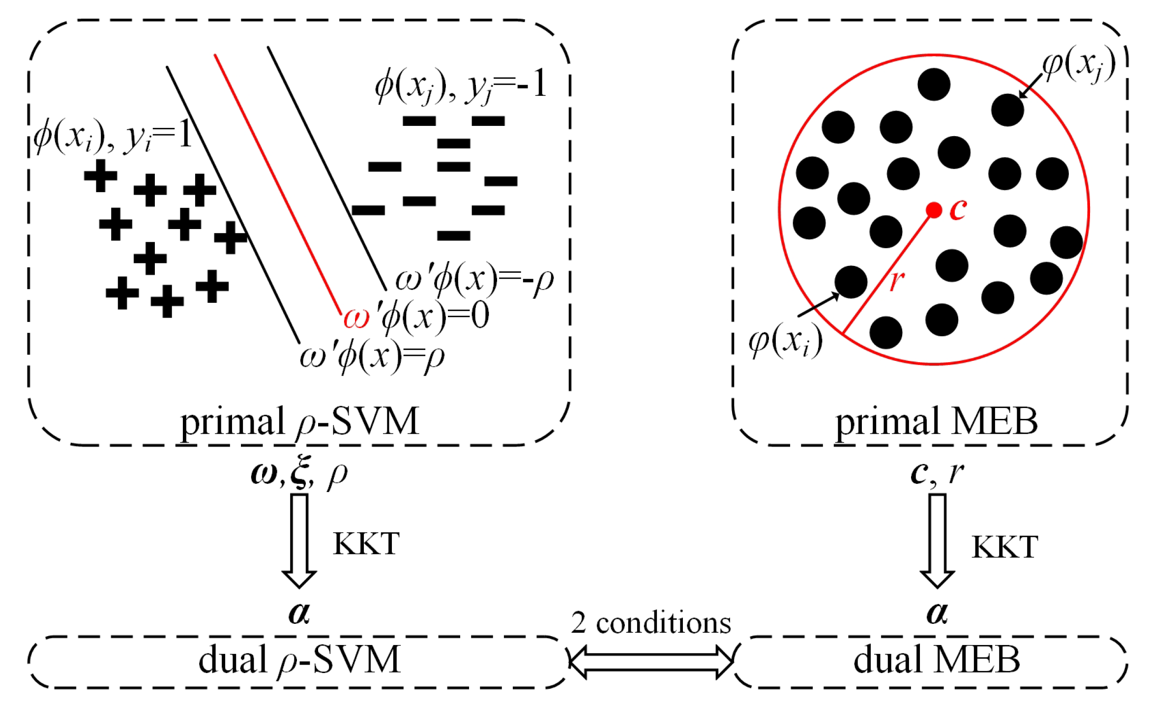
3.3. Equivalence of the SVM and MEB

The supervised $\rho$-SVM classification problem can be equivalently reformulated as an unsupervised MEB problem by encoding the label $y_i$ of sample ${\mathit{x}}_i$ in feature vector $\phi \left({\mathit{x}}_i\right)$. Specifically, the optimization problems of the dual $\rho$-SVM in Equation (2) and the dual MEB in Equation (6) are equivalent to each other if the following two conditions are satisfied [16,25]:

•     $\phi \left({\mathit{x}}_i\right)=[y_i\varphi \left({\mathit{x}}_i\right);{\mathit{e}}_i/\sqrt{C}]$
•     $k_{\varphi }({\mathit{x}}_i,{\mathit{x}}_i)={\kappa }_{\varphi },\forall {\mathit{x}}_i$

Here, ${\mathit{e}}_i$ denotes the N-dimensional one-hot column vector in which the ith element is 1 and all other elements are 0, while ${\kappa }_{\varphi }$ denotes a constant related to the kernel mapping function $\varphi (·)$.

When the kernel utilized by the MEB is $k_{\phi }$, the center $\mathit{c}$ and radius r of the MEB can be represented by $k_{\phi }$ and the mapping function $\phi$ according to Equation (7) in Section 3.2. Moreover, when these two conditions are satisfied, $k_{\phi }$ and $\phi$ can be substituted by another kernel $k_{\varphi }$ and mapping function $\varphi$. Therefore, the center $\mathit{c}$ and radius r can be represented by $k_{\varphi }$ and $\varphi$ after substitution, as listed in Equation (9). In other words, for any ${\alpha }_k\ne 0$, the center $\mathit{c}$ and radius r of the primal MEB can be represented by the solutions $\mathbf{\alpha }$ of $\rho$-SVM. The equivalence of $\rho$-SVM and the MEB are shown in Figure 1.

$$\mathit{c}=[\sum _{i=1}^N{\alpha }_i{y}_i\varphi \left({\alpha }_i\right);\frac{1}{\sqrt{C}}\sum _{i=1}^N{\alpha }_i{\mathit{e}}_i].$$

(9a)

$$\begin{array}{c}\hfill r=\sqrt{{\kappa }_{\varphi }+\frac{1}{C}-2(y_k\sum _{i=1}^N{\alpha }_i{y}_i{k}_{\varphi }({\mathit{x}}_i,{\mathit{x}}_k)+\frac{{\alpha }_k}{C})+\sum _{i=1}^N{\alpha }_i{\alpha }_j{y}_i{y}_j(k_{\varphi }({\mathit{x}}_i,{\mathit{x}}_j)+\frac{{\delta }_{ij}}{C})}.\end{array}$$

(9b)

4. Methodology

4.1. Motivation

According to Section 3, when the two conditions (see Section 3.3) are satisfied, a batch-mode classifier learned offline by the supervised convex optimization of the SVM can be attained by solving an unsupervised convex optimization of the MEB. In other words, a classifier can be equivalently transformed by a minimum enclosing ball. In view of such equivalence, a series of online SVM/MEB methods have been proposed in the literature to deal with the data in streams.

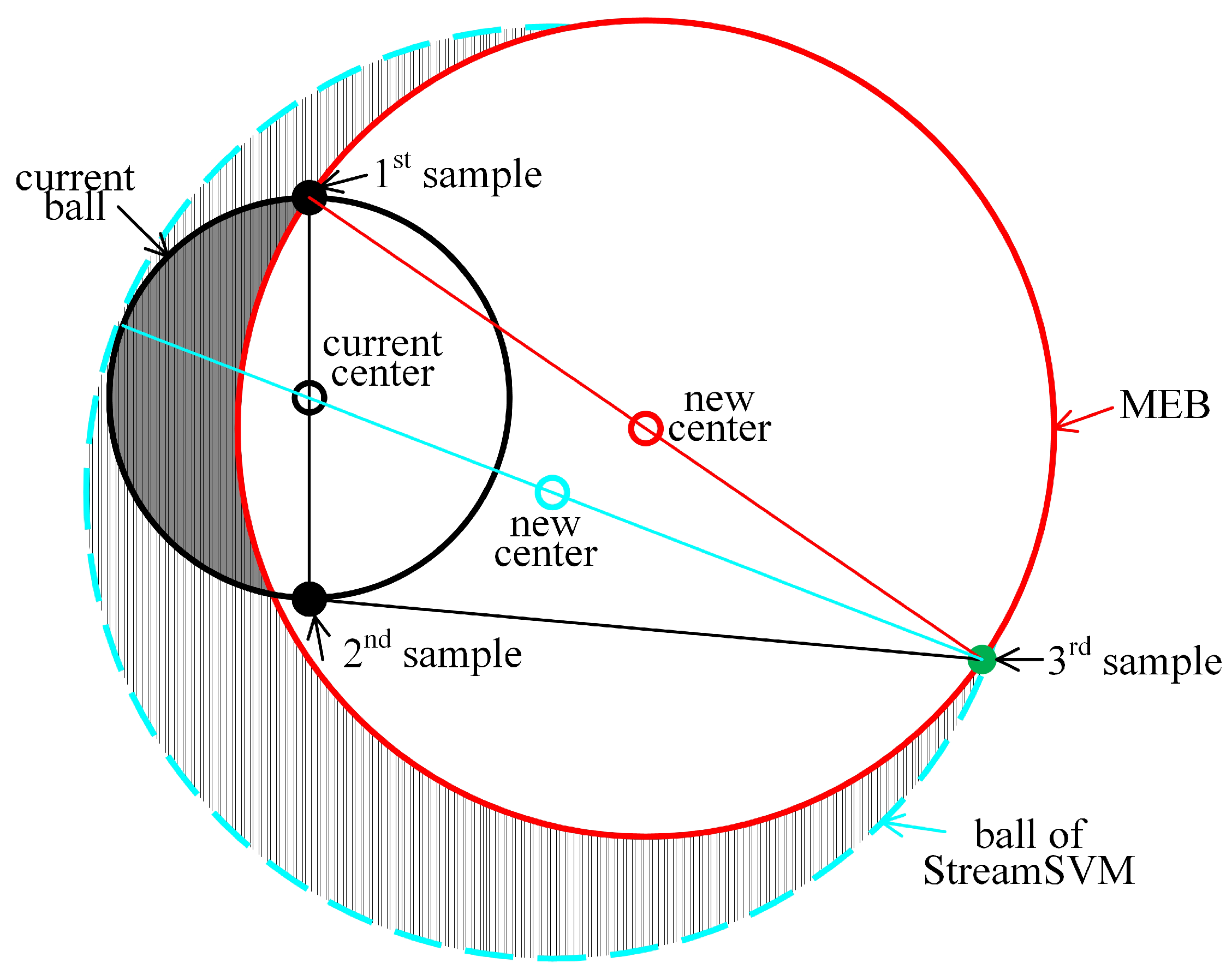
Taking the StreamSVM method in [16] as an example, a ball is constructed dynamically by enclosing all the streaming data. When a new sample arrives, StreamSVM learns a minimal ball enclosing both the sample and the current ball. Figure 2 illustrates the ball learned by StreamSVM when the third sample arrives outside. Although the enclosure of the whole current ball (the ball in black) instead of the old data (the first and second samples) prevents multiple passes of the data, it may lead to excessive enlargement of the ball (see the two colored balls for comparison). Because the ball of online methods often grows in an irreversible way, it ought to be enlarged cautiously in order to avoid enclosing any dispensable regions (e.g., the area with vertical lines as the background) as much as possible.

Therefore, we attempt to learn a new ball online under the constraint of a minimal radius with a single pass over the streaming data. To achieve this, we choose to relax the constraint of enclosing all data instead of the constraint of the minimal radius utilized by StreamSVM to avoid multiple passes. A new ball is required to enclose both the new sample and majority regions of the current ball, while the minority regions (e.g., the gray area in Figure 2) of the current ball are discarded, which are the regions most dissimilar to the new sample. On this basis, a new online method is proposed in the following section.

4.2. OSVM_SP

In Section 3.3, we introduce the equivalence between the MEB and $\rho$-SVM and show that the solutions $(\mathit{c},r)$ of the MEB can be equivalently represented by the solutions $\mathbf{\alpha }$ of the $\rho$-SVM according to Equation (9). In other words, if we can find a way to learn the MEB online, we can obtain its corresponding online classifier. The online learning of a decision hyperplane is equivalently transformed into the online learning of an MEB.

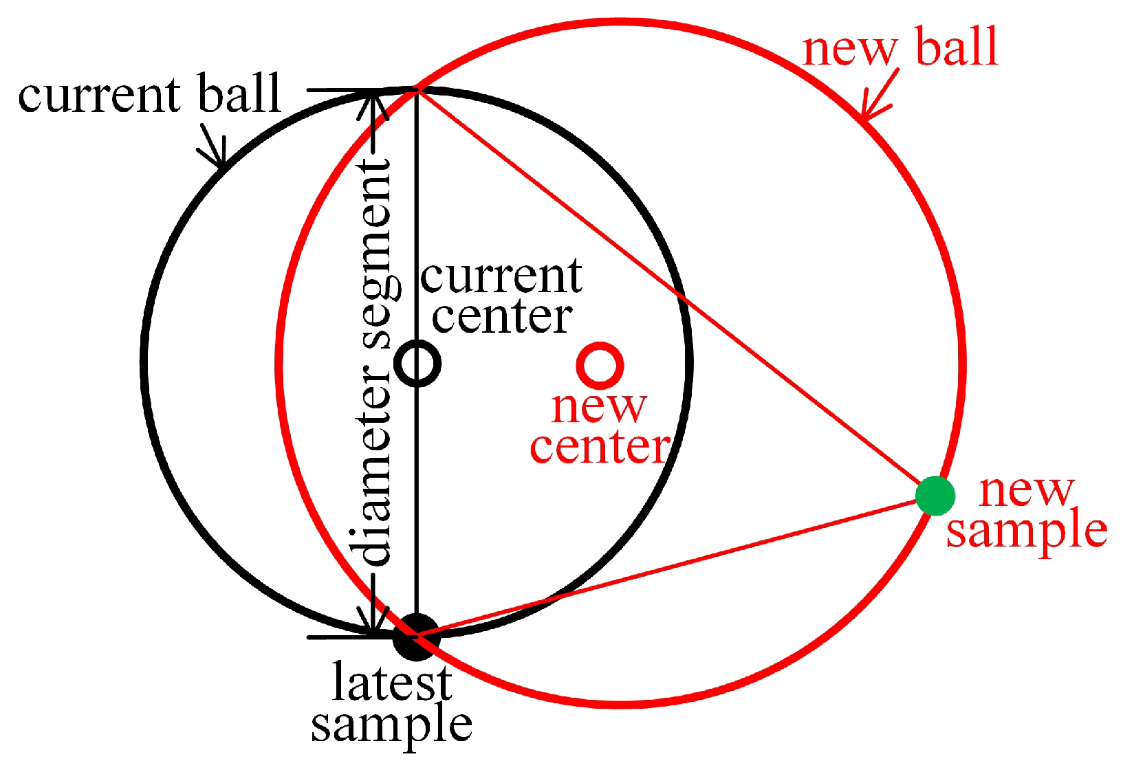
In this section, we present OSVM_SP, a new online SVM algorithm with a single pass over the streaming data. The basic idea of OSVM_SP is as follows: a ball is initialized by taking the first sample to arrive as the center and 0 as the radius; when a new sample arrives that is outside of the current ball, a new ball is learned to enclose both the sample and the majority of the region of the current ball with a radius increment that is as small as possible. To accomplish this, we record the latest sample that leads to the current ball being enlarged. Then, a diameter segment (see Figure 3) that crosses the recorded sample and the center of the current ball can be determined to represent the boundary of the majority of the region that must be enclosed in the new ball. Therefore, the new ball is created to enclose both the new sample and the diameter segment with a minimum radius.

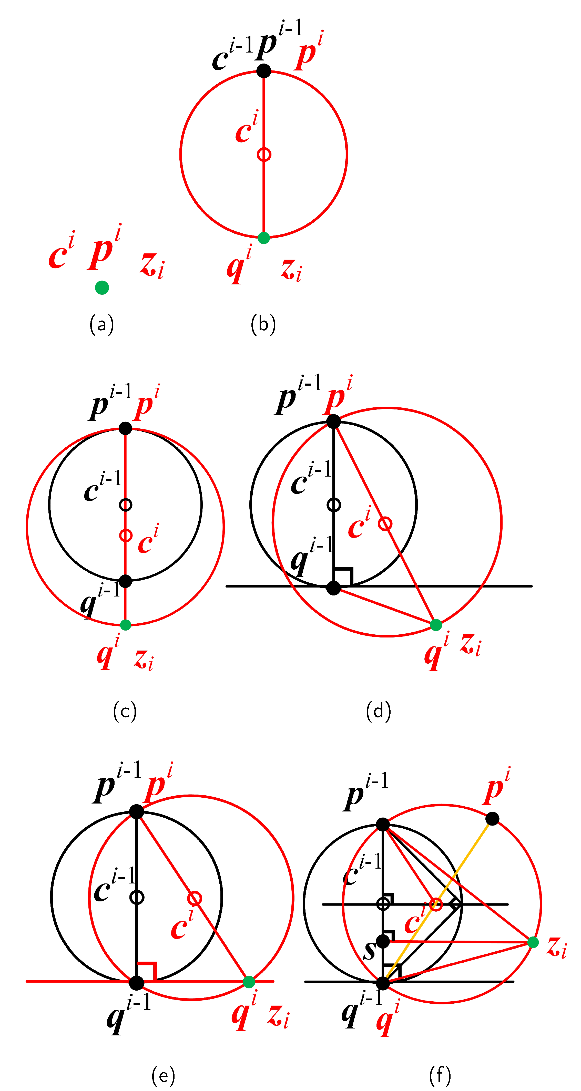
Before we elaborate on OSVM_SP, it is necessary to clarify the variables to be learned and the parameters required during the learning process. When the ith sample $({\mathit{x}}_i,y_i)$ arrives, $i=1,2,\cdots$ is first mapped into ${\mathit{z}}_i=\phi \left({\mathit{x}}_i\right)$ according to the first condition in Section 3.3. Let the current ball be $({\mathit{c}}^{i-1},r^{i-1})$ and $({\mathit{c}}^i,r^i)$ be the new ball to be learned. According to Equation (7a), the center ${\mathit{c}}^i$ can be represented as ${\mathit{c}}^i={\sum }_{j=1}^i{\alpha }_j^i{\mathit{z}}_j$ for each i. We use ${\mathit{p}}^{i-1}$ and ${\mathit{q}}^{i-1}$ to indicate two endpoints of the diameter segment (see Figure 4c–f), which can be universally expressed as ${\mathit{p}}^{i-1}={\sum }_{j=1}^{i-1}{\beta }_j^i{\mathit{z}}_j$ and ${\mathit{q}}^{i-1}={\sum }_{j=1}^{i-1}{\gamma }_j^i{\mathit{z}}_j$. Therefore, when the $i^{th}$ sample $({\mathit{x}}_i,y_i)$ arrives, online learning of the new ball $({\mathit{c}}^i,r^i)$ is equivalent to learning ${\mathbf{\alpha }}^i$, ${\mathbf{\beta }}^i$, ${\mathbf{\gamma }}^i$ and $r^i$ based on ${\mathbf{\alpha }}^{i-1}$, ${\mathbf{\beta }}^{i-1}$, ${\mathbf{\gamma }}^{i-1}$, $r^{i-1}$ and sample $({\mathit{x}}_i,y_i)$.

When $i=1$ and $({\mathit{x}}_i,y_i)$ is the first sample to arrive, we can easily initialize the MEB $({\mathit{c}}^i,r^i)$ to enclose the sole point ${\mathit{z}}_i$ by letting the center ${\mathit{c}}^i$ coincide with ${\mathit{z}}_i$ and the radius $r^i$ equal 0 (see Figure 4a). In addition, ${\mathit{z}}_i$ is recorded by considering ${\mathit{p}}^i$ as the sole end point, and ${\mathit{q}}^i$ is not available at the moment. See Steps 5–6 in Algorithm 1 for details.

$$\begin{array}{c}\hfill d({\mathit{z}}_i,{\mathit{c}}^{i-1})=\sqrt{\sum _{j,k=1}^{i-1}{\alpha }_j^{i-1}{\alpha }_k^{i-1}{y}_j{y}_k(k_{\varphi }({\mathit{x}}_j,{\mathit{x}}_k)+\frac{{\delta }_{jk}}{C})-2y_i\sum _{j=1}^{i-1}{\alpha }_j^{i-1}{y}_j{k}_{\varphi }({\mathit{x}}_j,{\mathit{x}}_i)+{\kappa }_{\varphi }+\frac{1}{C}}.\end{array}$$

(10)

When the ith sample $({\mathit{x}}_i,y_i)$ arrives for $i⩾2$, we first calculate the distance $d({\mathit{z}}_i,{\mathit{c}}^{i-1})$ in Equation (10) and compare it with the radius $r^{i-1}$ to determine whether ${\mathit{z}}_i$ is inside of the current ball $({\mathit{c}}^{i-1},r^{i-1})$. If it is, neither the ball nor the end points need to be adjusted, and they all inherit from the old ones (see Steps 24–26 in Algorithm 1); if not, a new ball $({\mathit{c}}^i,r^i)$ should be learned that encloses sample ${\mathit{z}}_i$ as well as the current end point(s). Derivations of Equation (10) have been listed in Appendix B for reference.

If ${\mathit{z}}_i$ is an outsider and the end point ${\mathit{q}}^{i-1}$ is unavailable, the new ball must enclose two points of end point ${\mathit{p}}^{i-1}$ and sample ${\mathit{z}}_i$, which can be easily learned by letting the center ${\mathit{c}}^i$ be the midpoint of these two points and letting $r^i$ equal half the distance between them (see Figure 4b). Additionally, sample ${\mathit{z}}_i$ is recorded by ${\mathit{q}}^i$, and ${\mathit{p}}^i$ inherits from ${\mathit{p}}^{i-1}$ in preparation for the next update. In this case, ${\mathbf{\alpha }}^i$, ${\mathbf{\beta }}^i$, ${\mathbf{\gamma }}^i$ and $r^i$ are computed by Equation (11).

$${\alpha }_j^i=\left\{\begin{array}{cc}\frac{1}{2}{\beta }_j^{i-1},\hfill & \forall j=1,\cdots ,i-1.\hfill \\ \frac{1}{2},\hfill & j=i.\hfill \end{array}\right.$$

(11a)

$${\beta }_j^i=\left\{\begin{array}{cc}{\beta }_j^{i-1},\hfill & \forall j=1,\cdots ,i-1.\hfill \\ 0,\hfill & j=i.\hfill \end{array}\right.$$

(11b)

$${\gamma }_j^i=\left\{\begin{array}{cc}0,\hfill & \forall j=1,\cdots ,i-1.\hfill \\ 1,\hfill & j=i.\hfill \end{array}\right.$$

(11c)

$$r^i=\frac{1}{2}d({\mathit{z}}_i,{\mathit{p}}^{i-1}).$$

(11d)

Algorithm 1 OSVM_SP

1: Input: ${({\mathit{x}}_i,y_i)}_{i=1,\cdots ,N}$, regularization parameter C, kernel function $k_{\varphi }({\mathit{x}}_i,{\mathit{x}}_j)$ with kernel parameter $\sigma$.

2: Output: Lagrange multiplier $\mathbf{\alpha }\in {\mathrm{R}}^{N\times 1}$.

3: for $i=1$ to N do

4:     Map sample $({\mathit{x}}_i,y_i)$ into ${\mathit{z}}_i$ according to ${\mathit{z}}_i=\phi \left({\mathit{x}}_i\right)=[y_i\varphi \left({\mathit{x}}_i\right);{\mathit{e}}_i/\sqrt{C}]$.

5:     if $i=1$ then             /*Initialization, see Figure 4a*/

6:          ${\alpha }_1^1\leftarrow 1$, ${\beta }_1^1\leftarrow 1$, ${\gamma }^1\leftarrow NaN$, $r^1\leftarrow 0$.

7:     else if $i⩾2$ then

8:       Compute $d({\mathit{z}}_i,{\mathit{c}}^{i-1})$, the distance of ${\mathit{z}}_i$ to the center ${\mathit{c}}^{i-1}$ of the current MEB, according to Equation (10).

9:       if $d({\mathit{z}}_i,{\mathit{c}}^{i-1})>r^{i-1}$ then

10:          if ${\mathbf{\gamma }}^{i-1}=NaN$ then                  /*See Figure 4b*/

11:            Compute ${\alpha }_j^i$, ${\beta }_j^i$, and ${\gamma }_j^i$ , $\forall j=1,\cdots ,i$, and $r^i$ according to Equation (11).

12:          else if ${\mathbf{\gamma }}^{i-1}\ne NaN$ then

13:              Compute $d({\mathit{z}}_i,{\mathit{p}}^{i-1})$ and $d({\mathit{z}}_i,{\mathit{q}}^{i-1})$, the distances of ${\mathit{z}}_i$ to the two end points of ${\mathit{p}}^{i-1}$ and ${\mathit{q}}^{i-1}$.

14:               if $d({\mathit{z}}_i,{\mathit{p}}^{i-1})⩽d({\mathit{z}}_i,{\mathit{q}}^{i-1})$ then                  /*Exchange $\mathbf{\beta }$ and $\mathbf{\gamma }$*/

15:                  $\mathbf{\beta }\leftrightarrows \mathbf{\gamma }$.

16:               end if

17:              Compute $cos\theta$ according to the cosine rule w.r.t. triangle ${\mathit{p}}^{i-1}{\mathit{q}}^{i-1}{\mathit{z}}_i$ with side lengths of $d({\mathit{z}}_i,{\mathit{p}}^{i-1})$, $d({\mathit{z}}_i,{\mathit{q}}^{i-1})$ and $2r^{i-1}$.

18:               if $cos\theta ⩽0$ then                  /*See Figure 4c–e*/

19:                  Compute ${\alpha }_j^i$, ${\beta }_j^i$, and ${\gamma }_j^i$ , $\forall j=1,\cdots ,i$, and $r^i$ according to Equation (11).

20:             else if$cos\theta >0$ then                     /*See Figure 4f*/

21:                  Compute ${\alpha }_j^i$, ${\beta }_j^i$, and ${\gamma }_j^i$ , $\forall j=1,\cdots ,i$, and $r^i$ according to Equation (12).

22:               end if

23:             end if

24:           end if$d({\mathit{z}}_i,{\mathit{c}}^{i-1})⩽r^{i-1}$ then

25:             ${\alpha }_i^i\leftarrow 0$, ${\beta }_i^i\leftarrow 0$, ${\gamma }_i^i\leftarrow 0$. ${\alpha }_j^i\leftarrow {\alpha }_j^{i-1}$, ${\beta }_j^i\leftarrow {\beta }_j^{i-1}$, ${\gamma }_j^i\leftarrow {\gamma }_j^{i-1}$, $\forall j=1,\cdots i-1$.

26:           end if

27:       end if

28: end for

29: return  $\mathbf{\alpha }=[{\alpha }_1^N;\cdots ;{\alpha }_N^N]$.

If ${\mathit{z}}_i$ is an outsider and the end point ${\mathit{q}}^{i-1}$ is available, the new ball must enclose all three points of ${\mathit{p}}^{i-1}$, ${\mathit{q}}^{i-1}$ and ${\mathit{z}}_i$. We assume that ${\mathit{p}}^{i-1}$ is the end point that is not less near sample ${\mathit{z}}_i$ than near ${\mathit{q}}^{i-1}$. If otherwise, we exchange the values of ${\mathit{\beta }}^{i-1}$ and ${\mathit{\gamma }}^{i-1}$ to satisfy the assumption. Let $\theta$ be $\angle {\mathit{p}}^{i-1}{\mathit{q}}^{i-1}{\mathit{z}}_i$, with $\theta \in (0,\pi ]$. According to the value of $\theta$, the construction of a new ball and the update process for the end points are divided into the following four subcases:

• $\theta =\pi$. The three points are collinear, and ${\mathit{q}}^{i-1}$ is between them (see Figure 4c). Therefore, the new ball $({\mathit{c}}^i,r^i)$ is constructed with the center being the midpoint of ${\mathit{p}}^{i-1}$ and ${\mathit{z}}_i$, and with the radius being equal to half their distance. Then, sample ${\mathit{z}}_i$ is recorded by ${\mathit{q}}^i$, and ${\mathit{p}}^i$ inherits from ${\mathit{p}}^{i-1}$. All these steps are performed according to Equation (11).
• $\theta \in (\pi /2,\pi )$. The three points constitute an obtuse triangle (see Figure 4d). A ball that encloses the two points ${\mathit{p}}^{i-1}$ and ${\mathit{z}}_i$ can enclose ${\mathit{q}}^{i-1}$ as well. Therefore, we can replicate the steps in the first subcase to fulfill the task.
• $\theta =\pi /2$. The three points constitute a right triangle (see Figure 4e). The ball constructed in the first subcase is simply the circumscribed sphere of the right triangle. Therefore, we can replicate the steps in the first subcase to fulfill the task.
• $\theta =(0,\pi /2)$. The three points constitute an acute triangle (see Figure 4f), and the new ball should be its circumscribed sphere. Therefore, ${\mathit{c}}^i$ and $r^i$ are set as the circumcenter and circumradius, respectively. Then, sample ${\mathit{z}}_i$ is recorded by ${\mathit{q}}^i$. As ${\mathit{c}}^i$ must be the midpoint of ${\mathit{p}}^i$ and ${\mathit{q}}^i$, ${\mathit{p}}^i$ can be obtained accordingly. Therefore, ${\mathbf{\alpha }}^i$, ${\mathbf{\beta }}^i$, ${\mathbf{\gamma }}^i$ and $r^i$ are computed by Equation (12).

$${\gamma }_j^i=\left\{\begin{array}{cc}0,\hfill & \forall j=1,\cdots ,i-1.\hfill \\ 1,\hfill & j=i.\hfill \end{array}\right.$$

(12a)

$$r^i=\frac{d({\mathit{z}}_i,{\mathit{p}}^{i-1})}{2sin\theta },{\beta }_j^i=2{\alpha }_j^i-{\gamma }_j^i.$$

(12b)

$$\begin{array}{c}\hfill {\alpha }_j^i=\left\{\begin{array}{c}(1-\frac{\sqrt{{\left(r^i\right)}^2-{\left(r^{i-1}\right)}^2}cos\theta }{r^{i-1}sin\theta }){\alpha }_j^{i-1}\hfill \\ +\frac{\sqrt{{\left(r^i\right)}^2-{\left(r^{i-1}\right)}^2}(d({\mathit{z}}_i,{\mathit{q}}^{i-1})cos\theta -r^{i-1})}{r^{i-1}sin\theta d({\mathit{z}}_i,{\mathit{q}}^{i-1})}{\gamma }_j^{i-1},\hfill & \forall j=1,\cdots ,i-1.\hfill \\ \frac{\sqrt{{\left(r^i\right)}^2-{\left(r^{i-1}\right)}^2}}{sin\theta d({\mathit{z}}_i,{\mathit{q}}^{i-1})},\hfill & j=i.\hfill \end{array}\right.\end{array}$$

(12c)

The online learning process of OSVM_SP is provided in Algorithm 1. Whenever there is a label prediction requirement, an optimal hyperplane equivalent to the current ball can be generated accordingly by Equation (4).

The most time-consuming steps in Algorithm 1 are the distance computations in Steps 8 and 13. Among them, the distance to center $d({\mathit{z}}_i,{\mathit{c}}^{i-1})$ in Step 8 must be computed for every upcoming ${\mathit{z}}_i$, whereas $d({\mathit{z}}_i,{\mathit{p}}^{i-1})$ and $d({\mathit{z}}_i,{\mathit{q}}^{i-1})$ in Step 13 need to be computed only under certain conditions (see Steps 9 and 12). Note that the space requirement of OSVM_SP grows without limit as the data continue to arrive, which might be infeasible in high-rate data streams.

4.3. Budgeted OSVM_SP

For the aforementioned reason, we propose three budgeted versions of OSVM_SP to decrease the boundless space requirement. Specifically, a budget of fixed size is utilized as the upper bound of the storage space. When this budget is exceeded, it is necessary to remove an SV learned beforehand to make space for the new SV. Therefore, our budgeted algorithms all have constant space complexity. The core of budgeted algorithms is the method of choosing the SV to remove. We employ three widely used SV removal principles [26,27] to remove either a randomly selected SV (-Ran), the oldest SV (-Old), or the least important SV (-Min). Here, the importance of an SV is measured by the value of its corresponding multiplier. Accordingly, the three proposed budgeted versions of OSVM_SP are denoted OSVM_SP-Ran, OSVM_SP-Old, and OSVM_SP-Min.

4.4. Complexity Analysis

The respective time and space complexities of OSVM_SP are $O\left(N^2\right)$ and $O(N^2+Nd)$. Let B be the size of the budget; then, the time complexity of our three budgeted algorithms (OSVM_SP-Ran, OSVM_SP-Old, and OSVM_SP-Min) is $O\left(NB\right)$ and the space complexity is $O(B^2+Bd)$, a constant unrelated to the number of samples N.

Note that when the linear kernel is employed in OSVM_SP, both the center and the two end points can be explicitly computed and stored for computing the distances in Steps 8 and 13. In such a case, OSVM_SP has $O\left(d\right)$ space complexity, which is unrelated to the sample number N or time complexity $O\left(N\right)$.

Table 1. Computational complexity of the proposed methods.

Method	Time	Space
OSVM_SP	$O\left(N^2\right)$	$O(N^2+Nd)$
Three Budgeted OSVM_SPs	$O\left(NB\right)$	$O(B^2+Bd)$
OSVM_SP with linear kernel	$O\left(N\right)$	$O\left(d\right)$

lists the computational complexity of all the methods.

4.5. Comparison of OSVM-SP with StreamSVM

When the first training sample arrives, OSVM-SP and StreamSVM both initialize a ball of $({\mathit{z}}_i,0)$. When the first sample arrives and is outside of the current ball, OSVM-SP and StreamSVM both construct a new ball of $(\mathrm{midpoint},\mathrm{distance}/2)$ to replace the current ball. When the third or later sample arrives outside, however, the balls of OSVM-SP and StreamSVM may coincide with each other in certain cases, although most of the time they differ from each other.

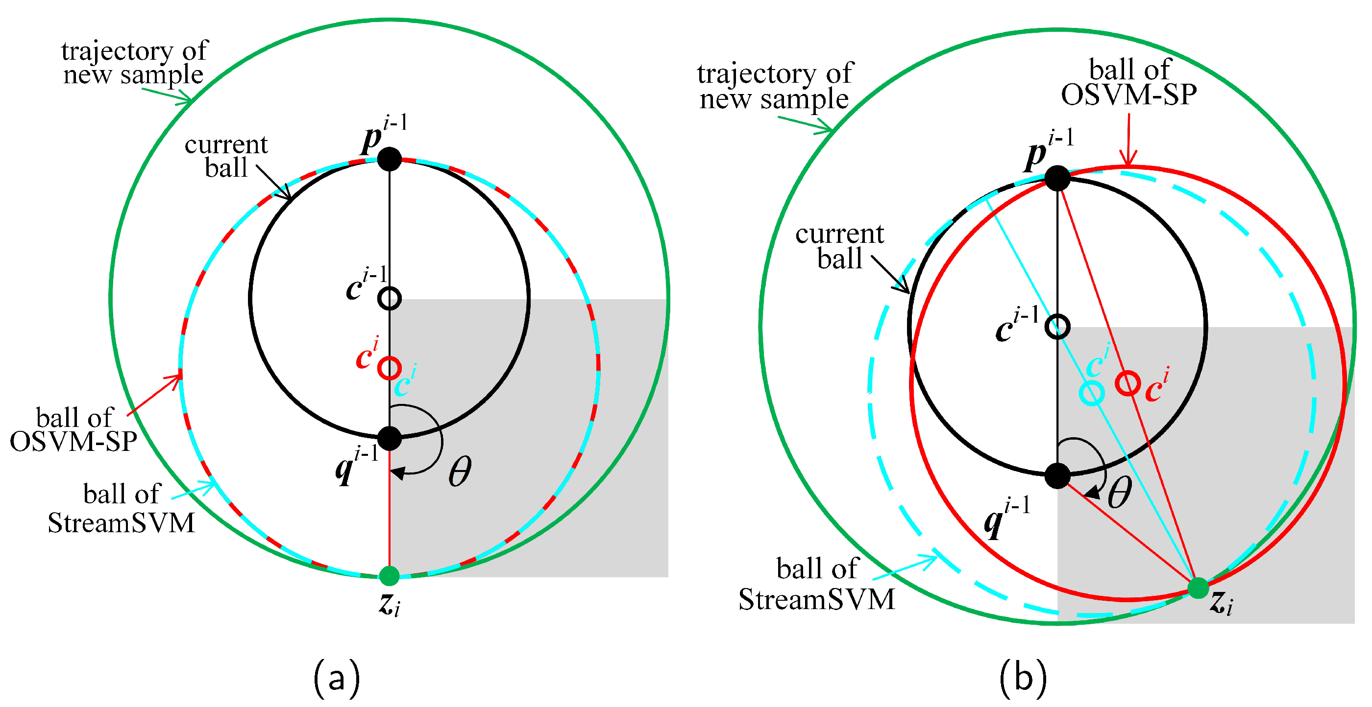
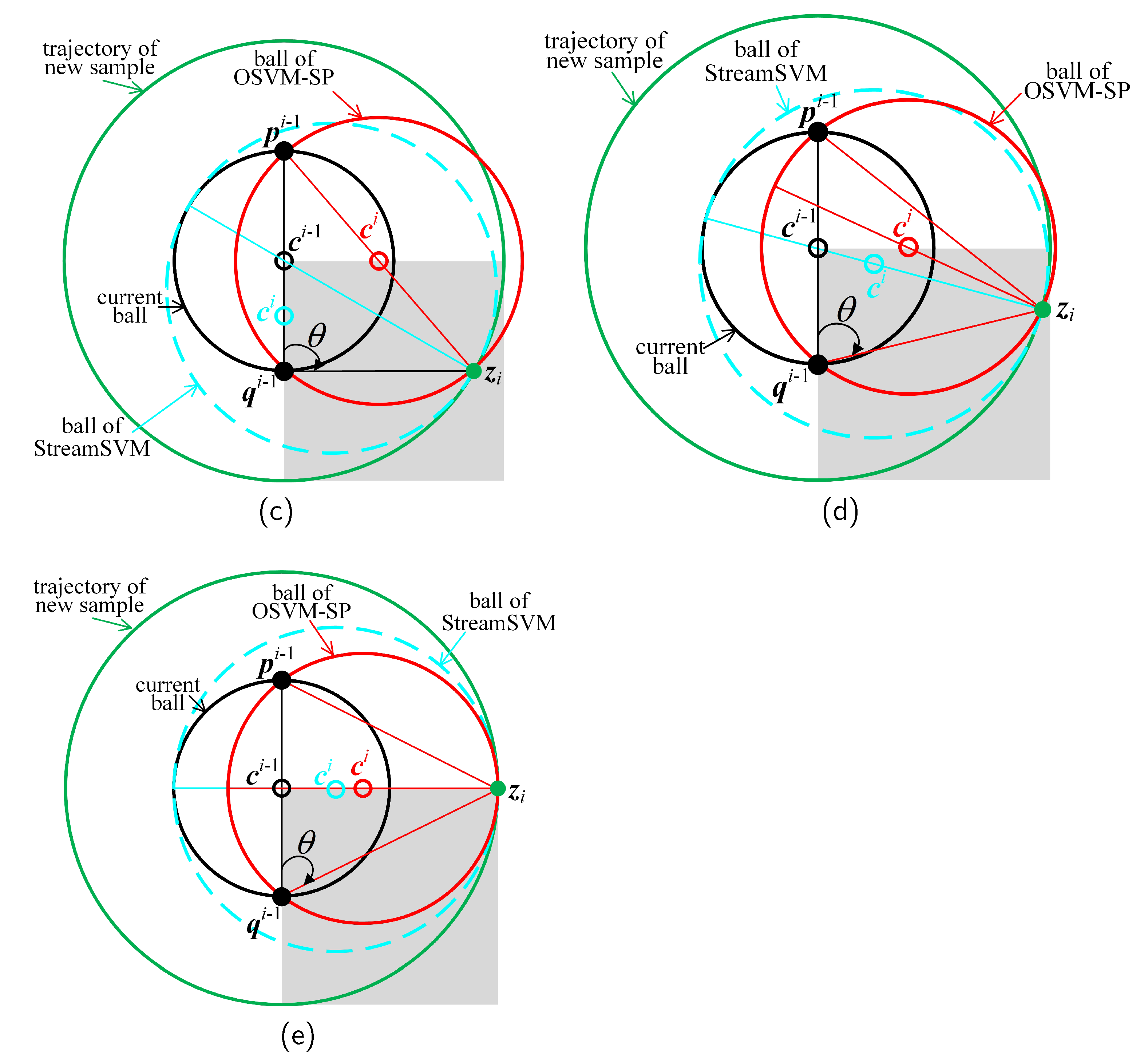
Figure 5 illustrates a comparison of OSVM-SP with StreamSVM in the construction of new balls, while ${\mathit{z}}_i$ denotes the third or later sample coming outside of the current ball $({\mathit{c}}^{i-1},r^{i-1})$ (the ball in black); hence, $d({\mathit{z}}_i,{\mathit{c}}^{i-1})>r^{i-1}$. For convenience of analysis, the distance $d({\mathit{z}}_i,{\mathit{c}}^{i-1})$ is equal to a constant $d_{const}$; therefore, the trajectory of all the possible ${\mathit{z}}_i$ is a ball denoted $({\mathit{c}}^{i-1},d_{const})$ (the ball in green). Because the trajectory is bilaterally symmetric, only the left or right half of the trajectory must be considered. Moreover, if we continue to assume that ${\mathit{q}}^{i-1}$ is the end point closer to sample ${\mathit{z}}_i$ than ${\mathit{p}}^{i-1}$, then only a quarter of the trajectory (the green ball with the gray background) is distinguished for consideration.

Figure 5a–e illustrates five different cases in which the new sample ${\mathit{z}}_i$ may appear in the trajectory, divided according to the value of angle $\theta$. When $\theta =\pi$ and sample ${\mathit{z}}_i$ is co-linear to the endpoints (see Figure 5a), new balls of OSVM-SP (the ball in red) and StreamSVM (the ball in dotted blue) coincide with each other; otherwise, these two balls are different (see Figure 5b–d). In particular, when $\theta =\pi /4$ and the distances from sample ${\mathit{z}}_i$ to those end points are equal (see Figure 5e), the new ball of OSVM-SP is enclosed by the new ball of StreamSVM.

5. Experiments

5.1. Benchmark Datasets

Six binary datasets (australian, fourclass, banknote, svmguide1, EGSSD, and occupation) were employed to validate the performance of our methods; they are all publicly available from the following websites (https://archive.ics.uci.edu/ml/datasets, accessed on 1 January 2022; https://www.csie.ntu.edu.tw/~cjlin/libsvmtools/datasets, accessed on 1 January 2022). Each dataset had already been scaled featurewise to (−1,1) according to min–max normalization. All of the datasets contained only one set of data, except for svmguide1, which contained two sets of training and testing data. We merged these two sets into a single set for unified management during the following experiments, making svmguide1 the same as the remaining datasets. The specifications of the datasets are listed in

Table 2. Specifications of the public datasets.

Dataset	# Features	#Instances	Majority%
australian	14	690	55.51
fourclass	2	862	64.39
banknote	4	1372	55.54
svmguide1	4	7089	56.43
EGSSD	13	10,000	63.80
occupation	5	20,560	76.90

, showing the number of features, sample size, and percentage of the majority class contained in each dataset. The missing data issue does not exist in these six datasets as the online methods we focus on in this paper are not able to handle the missing data problem, although this might be an interesting and promising research direction in future work.

5.2. Baseline Methods

The proposed method is denoted as OSVM_SP, while OSVM_SP-Ran, OSVM_SP-Old, and OSVM_SP-Min are three budgeted versions of OSVM_SP that respectively remove a randomly selected SV, the oldest SV, and the least important SV when the budget is exceeded. The methods for comparison can be divided into three groups: “nonbudgeted online”, “budgeted online”, and “offline”. The nonbudgeted online group consists of five methods (StreamSVM, PA, PA-I, PA-II, and AMM-online), which are mainly compared with the proposed OSVM_SP. Meanwhile, the two budgeted online representatives (BSGD and BPA-S) are compared with OSVM_SP-Ran, OSVM_SP-Old, and OSVM_SP-Min. The two offline batch methods (SVM and $\rho$-SVM) are listed as the baselines. Nine comparable methods are briefly introduced below.

-

StreamSVM [16]: StreamSVM is a nonbudgeted online method that leverages the equivalence of SVM and MEB (see Section 3.3), which is similar to our OSVM_SP method. For any incoming point outside of the ball, the StreamSVM algorithm moves the center towards it and simultaneously enlarges the radius to cover both the point and the previous ball. OSVM_SP is different from StreamSVM in that the center moves in different directions and the radius grows according to different strategies; see Figure 4d–f. Taking Figure 4e as an example, the two directions ${\mathit{c}}^{i-1}$ to ${\mathit{z}}_i$ (in StreamSVM) and ${\mathit{c}}^{i-1}$ to $({\mathit{p}}^{i-1}+{\mathit{z}}_i)/2$ (in OSVM_SP) are very different from each other.

-

PA, PA-I, and PA-II [17]: PA, PA-I, and PA-II are three nonbudgeted online algorithms operating under the same framework provided in [17], which formalizes the trade-off between the correct classification of new data with a sufficiently high margin and the amount of information retained from old data. Among them, PA is a hard margin classifier while PA-I and PA-II are soft margin classifiers with losses of ℓ1 and ℓ2, respectively.

-

AMM-online [28]: another nonbudgeted algorithm, AMM-online is an online version of AMM that consists of a set of hyperplanes; each hyperplane is assigned to one class. We employ the implementation of AMM-online in the BudgetedSVM toolbox [29]. Note that the default setting of AMM-online in the toolbox is required to run five training epochs, which deviates from the restriction of single-pass online learning. In fact, we tried to run AMM-online in one epoch; however, its performance declined rapidly. Therefore, the performance of AMM-online with five epochs is listed in all the following experimental results.

-

BSGD [27]: BSGD is a class of budgeted versions of online SVM algorithms that belong to the SGD family. We employ the implementation of BSGD in the same BudgetedSVM toolbox with two budget maintenance strategies, “-removal” and “-merging”, which are based on the removal and merging of support vectors during the training process. The experimental results based on our six datasets show that there is a minor difference between these methods.

-

BPA-S [26]: BPA-S is a budgeted version of PA-I. When the budget is exceeded, BPA-S removes an SV to make room for the new sample, while the multipliers of the remaining SV remain unchanged.

-

ρ-SVM & SVM: $\rho$-SVM is the respective offline batch method corresponding to our OSVM_SP, introduced in Section 3.1. We implemented the dual $\rho$-SVM in Equation (2) with convex optimization (CVX) [30,31], a package for specifying and solving convex programs. The SVM indicates the corresponding offline model of StreamSVM, which is a transformation of $\rho$-SVM in which the variable $\rho$ is set to a constant value of 1.

5.3. User-Specified Parameters

For simplicity, we utilize the Gaussian kernel $k({\mathit{x}}_i,{\mathit{x}}_j)=exp({\parallel {\mathit{x}}_i-{\mathit{x}}_j\parallel }^2/\sigma )$ for all the kernelized methods, as it satisfies the 2^nd condition in Section 3.3. Therefore, the penalty parameter C and kernel parameter $\sigma$ must be set for StreamSVM, PA, PA-I, PA-II, SVM, $\rho$-SVM, and the proposed OSVM_SP, OSVM_SP-Ran, OSVM_SP-Old, and OSVM_SP-Min. As the SVM and $\rho$-SVM are the corresponding batch versions of StreamSVM and OSVM_SP, they share the same objective functions. Therefore, SVM is utilized to choose the optimal parameter values for StreamSVM as well as itself, and $\rho$-SVM is utilized both for itself and the proposed four methods. The optimal group $(C^{\ast },{\sigma }^{\ast })$ is chosen by performing a grid search with $\{2^{-10},2^{-9},\cdots ,2^9,2^{10}\}\times \{2^{-10},2^{-9},\cdots ,2^9,2^{10}\}$. Because there is no explicit batch-mode optimization problem for PA, PA-I, or PA-II, there is no corresponding batch model in the experiments. The values of parameters C and $\sigma$ within these three methods are set according to the SVM.

The parameter values corresponding to the best performance were chosen as the optimal values, and are listed in

Table 3. Optimal parameter values after grid search.

	SVM		$\mathit{\rho }$-SVM
	${\mathit{C}}^{\ast }$	${\mathbf{\sigma }}^{\ast }$	${\mathit{C}}^{\ast }$	${\mathbf{\sigma }}^{\ast }$
australian	$2^{-9}$	$2^0$	$2^{-1}$	$2^1$
fourclass	$2^{-10}$	$2^{-8}$	$2^{-10}$	$2^{-6}$
banknote	$2^0$	$2^{-3}$	$2^1$	$2^{-1}$
svmguide1	$2^6$	$2^{-3}$	$2^{-2}$	$2^{-3}$
EGSSD	$2^0$	$2^1$	$2^{-2}$	$2^1$
occupation	$2^{-3}$	$2^{-5}$	$2^{-6}$	$2^{-4}$

for each dataset. Each dataset was randomly divided into training and testing sets according to two-fold cross-validation. A series of SVM and $\rho$-SVM models were learned based on the training set with different parameter values, and their classification accuracies were measured based on the testing set.

The experiments in the following subsections were all conducted as follows: each dataset was randomly divided into equal-sized training and testing sets; every method in Section 5.2 was trained with the former set and validated with the latter set; we ran each method five times with randomized permutations, and reported the mean results (along with the standard deviation in several subsections) from the experiments.

5.4. Classification Accuracy

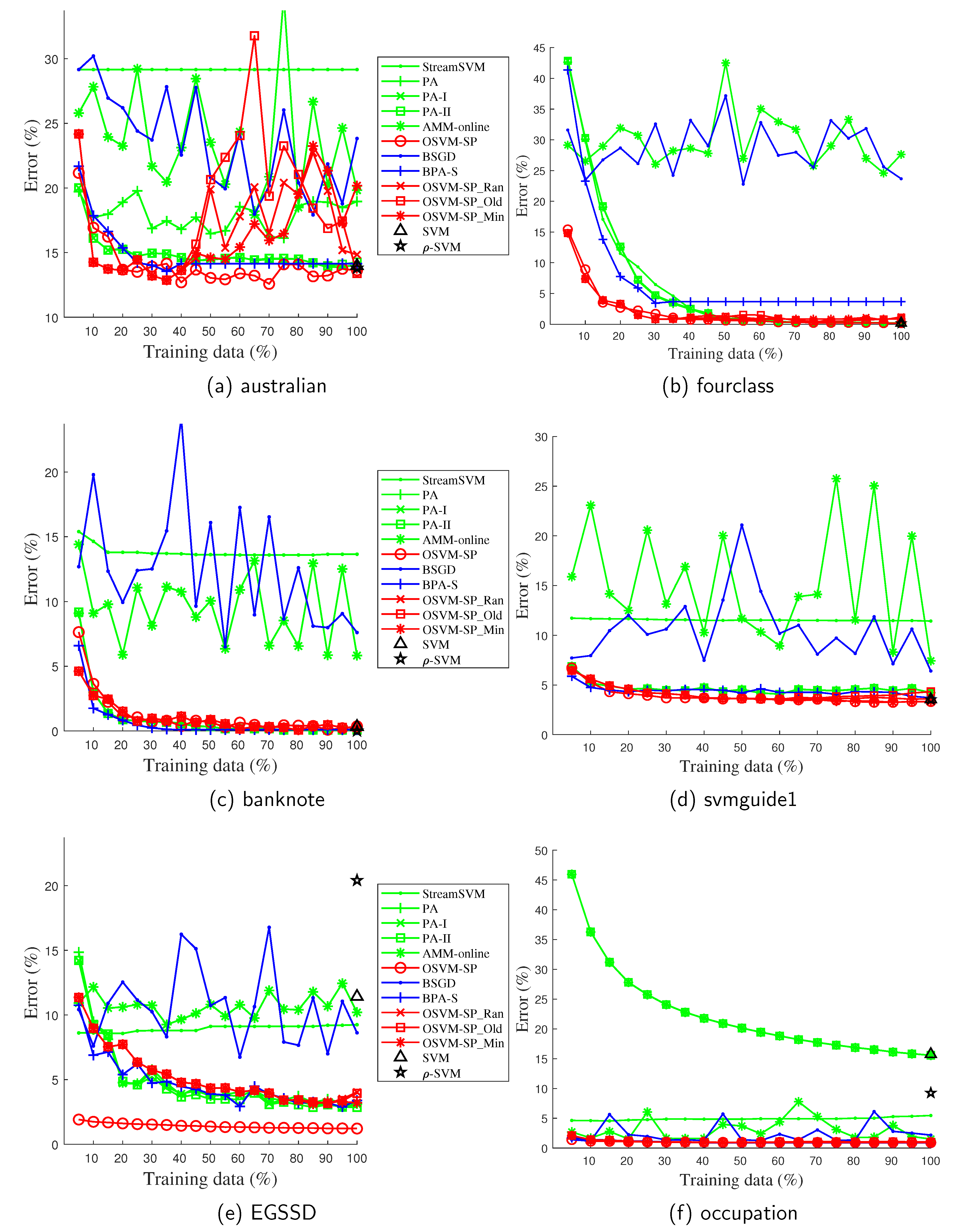
First, we validated the predictive performance of all the methods based on six datasets. This paper focuses on training online models over streaming data, which means that training samples arrive one by one or chunk by chunk. Whenever a new sample arrives, the current model may require a timely update to fit the new sample. Therefore, online models usually change dynamically and frequently during the whole training process. The trend in the performance of an online model is of great importance, as it clearly reflects whether, or even how, the model adapts to the new data. The performance comparison of online models with respect to different sizes of training data is an easy way of displaying the trends, and is widely utilized by many state-of-the-art online learning-related methods [32,33,34,35]. Figure 6 shows the classification error with respect to different amounts of training data, while

Table 4. Classification accuracy (mean ± STD, %) with best results shown in bold.

	Methods	Datasets
		Australian	Fourclass	Banknote	Svmguide1	EGSSD	Occupation
non-budgeted online	StreamSVM	70.8 ± 8.0	99.8 ± 0.2	86.4 ± 11.0	88.6 ± 2.3	90.8 ± 0.8	94.5 ± 1.6
	PA	81.0 ± 2.9	99.8 ± 0.2	99.9 ± 0.1	95.8 ± 0.3	96.9 ± 0.4	84.4 ± 0.3
	PA-I	86.0 ± 0.5	99.8 ± 0.2	99.9 ± 0.1	95.8 ± 0.3	96.9 ± 0.7	84.4 ± 0.3
	PA-II	85.7 ± 0.7	99.8 ± 0.2	99.9 ± 0.1	95.8 ± 0.3	97.1 ± 0.5	84.4 ± 0.3
	AMM-online	80.2 ± 8.3	72.4 ± 7.1	94.2 ± 2.8	92.6 ± 1.5	89.8 ± 2.0	98.5 ± 0.3
	OSVM-SP	86.4 ± 0.9	99.8 ± 0.2	99.7 ± 0.2	96.7 ± 0.1	98.8 ± 0.1	99.1 ± 0.0
budgeted online	BSGD	76.2 ± 13.1	76.3 ± 3.0	92.4 ± 3.7	93.6 ± 1.8	91.4 ± 4.8	97.8 ± 2.1
	BPA-S	85.9 ± 2.0	96.3 ± 1.5	99.9 ± 0.1	96.3 ± 0.2	96.6 ± 1.6	99.1 ± 0.1
	OSVM-SP_Ran	85.2 ± 2.5	98.8 ± 0.9	99.7 ± 0.3	96.4 ± 0.4	96.0 ± 2.1	99.0 ± 0.1
	OSVM-SP_Old	86.6 ± 1.4	98.9 ± 0.9	99.7 ± 0.3	95.7 ± 0.5	96.1 ± 1.3	99.0 ± 0.1
	OSVM-SP_Min	79.8 ± 5.3	99.2 ± 0.7	99.7 ± 0.3	96.7 ± 0.4	96.8 ± 0.8	99.1 ± 0.1
offline	SVM	86.0 ± 1.6	99.8 ± 0.2	99.7 ± 0.3	96.5 ± 0.3	88.6 ± 1.1	84.3 ± 0.4
	$\rho$-SVM	86.2 ± 1.9	99.9 ± 0.2	100.0 ± 0.0	96.5 ± 0.2	79.6 ± 1.5	90.7 ± 0.3

lists the classification accuracy attained at the end of the training process.

OSVM_SP obtains the highest accuracy among the six nonbudgeted online methods for nearly all the datasets, with the exception of banknote, for which it is surpassed by PA, PA-I, and PA-II with a slight accuracy loss (0.2%). In addition, PA, PA-I, and PA-II share the highest accuracy with OSVM_SP based on the fourclass dataset. The budgeted versions of OSVM_SP, OSVM_SP-Ran, OSVM_SP-Old, and OSVM_SP-Min converge steadily to OSVM_SP in predictive performance for all six datasets. In fact, there is a slight accuracy loss for OSVM_SP-Min based on fourclass and EGSSD compared with OSVM_SP, which seems reasonable as OSVM_SP-Min must occasionally remove SVs in order to make room for the new sample. Despite the accuracy loss, OSVM_SP-Min surpasses the other budgeted online methods (BSGD and BPA-S) most of the time. OSVM_SP-Old beats OSVM_SP-Min and even OSVM_SP based on the australian dataset, achieving the best performance only this once. The superiority of OSVM_SP-Ran does not appear obvious, indicating that an SV removal principle with more explicit intentionality might be more helpful than randomization. The difference in accuracy between the two batch-mode algorithms, the SVM and $\rho$-SVM, is negligible for most of the datasets. The error of PA increases and then decreases for the australian dataset, while PA-I and PA-II behave much more steadily for all six datasets. PA-I and PA-II are soft margin classifiers that enable misclassification of several training samples, whereas the hard margin classifier, PA, does not. Therefore, we suspect that PA might be sensitive to noise in the data. StreamSVM obtains the best results for fourclass, although it fails for the remaining datasets. Moreover, the performance of StreamSVM remains at a nearly static level, with no further improvement during the training process for the remaining five datasets. This result is analyzed in Section 5.5.

5.5. Percentage of Support Vectors

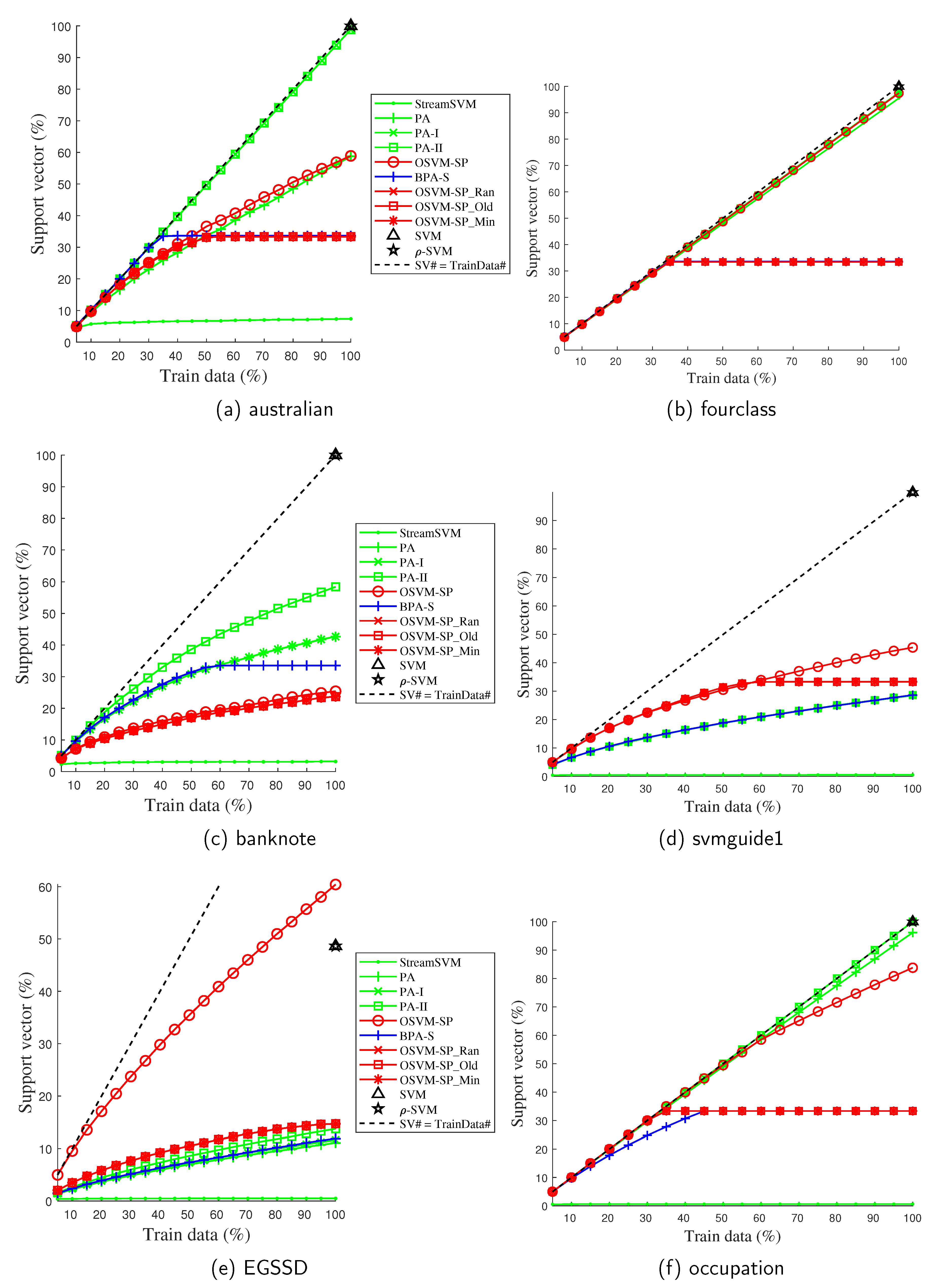
Our second experiment examined the computation and memory requirements of each method by counting the percentage of SVs in the training data during the whole training process. As the proposed OSVM_SP and its three budgeted versions along with the majority of the compared methods are kernelized, the number of SVs can be considered one of the most important indicators of computation and memory consumption. Here, an SV is denoted as a training sample with a nonempty Lagrange multiplier. Figure 7 depicts the number of SVs with respect to different amounts of training data.

For most unbudgeted online methods, the number of SVs increases with the amount of training data. The curve for OSVM-SP varies greatly between different datasets. When the amount of training data approaches 100%, however, the number of SVs for OSVM-SP remains less than (see Figure 7a,c,d,f) or as much as (see Figure 7b) the SV numbers of the SVM and $\rho$-SVM in most cases. In combination with the accuracy results in Table 4, the effective predictive performance of SVM and $\rho$-SVM is acquired at a cost of nearly 100% of the training data, as the SVs (see Figure 7a–d) can consume enormous amounts of memory and time latency in both the model training and label prediction processes. Compared with SVM and $\rho$-SVM, OSVM-SP is more lightweight while attaining a comparable predictive performance. Sometimes, OSVM-SP even achieves higher accuracy (10.2–19.2%, see Table 4) than the batch methods, although at the cost of more SVs (see Figure 7e). PA generates fewer SVs than PA-II and/or PA-I most of the time (see Figure 7a,c,e,f), which is to be expected as the SVs of the hard margin method PA consist of only the misclassified data, while the SVs of the soft margin methods PA-I and PA-II are constructed using both the misclassified data and those that are classified correctly and are within the margin. StreamSVM maintains a small number of SVs based on five datasets, with the exception of fourclass. In combination with the accuracy results of StreamSVM in Table 4, the reason for this might be that the corresponding MEB of StreamSVM expands excessively to cover most of the training data arriving afterwards without triggering any further updates.

For the budgeted online methods, the number of SVs initially increases with the amount of training data. When it grows to the size of the budget (one-third of the training size), it remains constant through the various SV removal principles utilized. The number of SVs for OSVM_SP-Ran, OSVM_SP-Old, and OSVM_SP-Min is controlled in keeping with the size of the budget. Compared with the nonbudgeted OSVM_SP, it can bes observed that decreasing the memory requirement by approximately two-thirds leads to only a 0.6–2.0% loss in accuracy. In other words, OSVM_SP-Ran, OSVM_SP-Old, and OSVM_SP-Min offer great potential for efficiency and effectiveness in budgeted online learning.

5.6. Radius of the Minimum Enclosing Ball

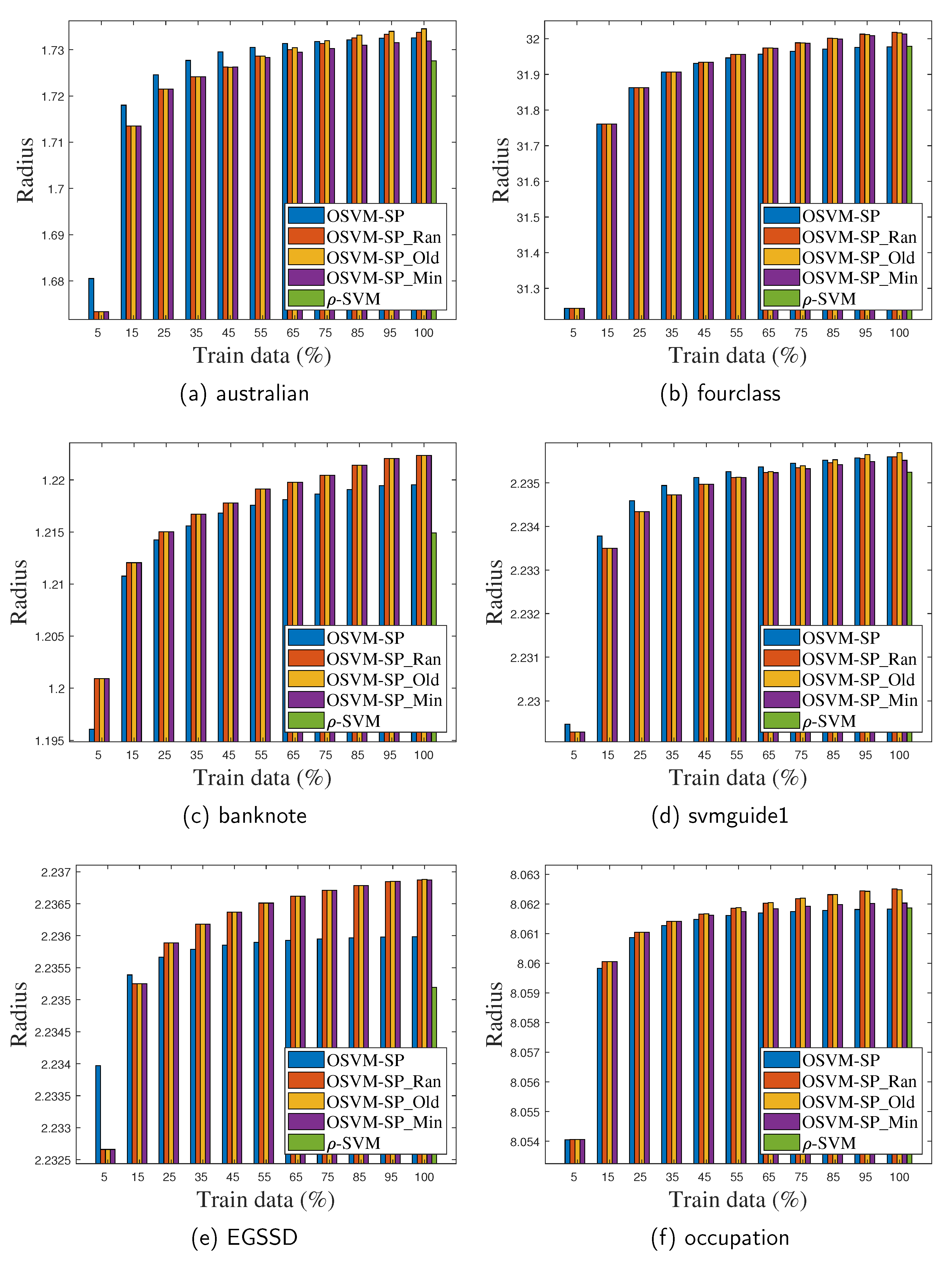
Our third experiment compared the radii of the MEBs corresponding to the proposed nonbudgeted online method (OSVM_SP), the three budgeted online methods (OSVM_SP-Ran, OSVM_SP-Old and OSVM_SP-Min), and the corresponding batch-mode method ($\rho$-SVM). Figure 8 shows the radii with respect to different amounts of training data.

The methods can be sorted in ascending order of radii, that is, $\rho$-SVM, OSVM_SP, OSVM_SP-Min, OSVM_SP-Old, and OSVM_SP-Ran, on each dataset. The batch-mode method, $\rho$-SVM, achieves the minimum radius, as it can iteratively search for the smallest ball among those covering all the training data. OSVM_SP falls between the batch-mode $\rho$-SVM and the three budgeted online methods. In Figure 4f, the ball with respect to OSVM_SP can be determined by three points represented by two real samples (${\mathit{q}}^i$ and ${\mathit{z}}^i$) and one fake sample (${\mathit{p}}^i$), which we believe incurs an expanding radius as well as a loss in accuracy. The budgeted online methods obtain a larger radius than OSVM_SP, as one SV must be removed whenever the budget is exceeded. Because the center of the ball is linearly represented by the SVs, the center drifts away from the location it had after the removal. Therefore, these methods have to enlarge their radii to cover the new data. In addition, the degree of drift varies for different removal principles. Among these budgeted online methods, OSVM_SP-Min achieves the minimal radius mostly by removing the least important SV, while OSVM_SP-Ran or OSVM_SP-Old achieves the maximal radius by removing a randomized SV or the oldest SV. There is occasionally a minor difference in their radius lengths.

5.7. Effect of Budget Size

Our last experiment verified the effect of different budget sizes on the performance of the three proposed budgeted methods, OSVM_SP-Ran, OSVM_SP-Old, and OSVM_SP-Min. The size of the budget was set to be a range of percentages of the training data, with the percentage chosen by a grid search with $(5\%,10\%,\cdots ,95\%,100\%)$. Note that when the percentage equals 100%, OSVM_SP-Ran, OSVM_SP-Old, and OSVM_SP-Min are identical to OSVM_SP, which means that the budget is able to store all the training data without any SVs needing to be removed.

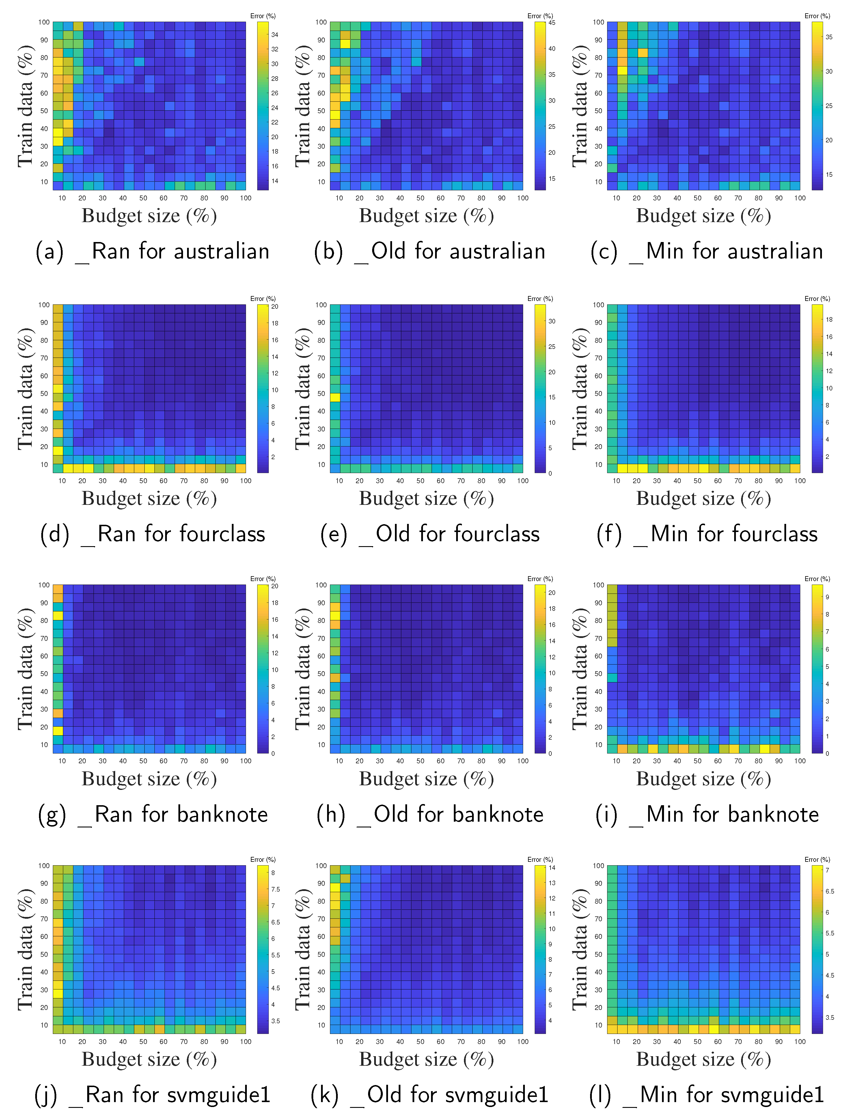
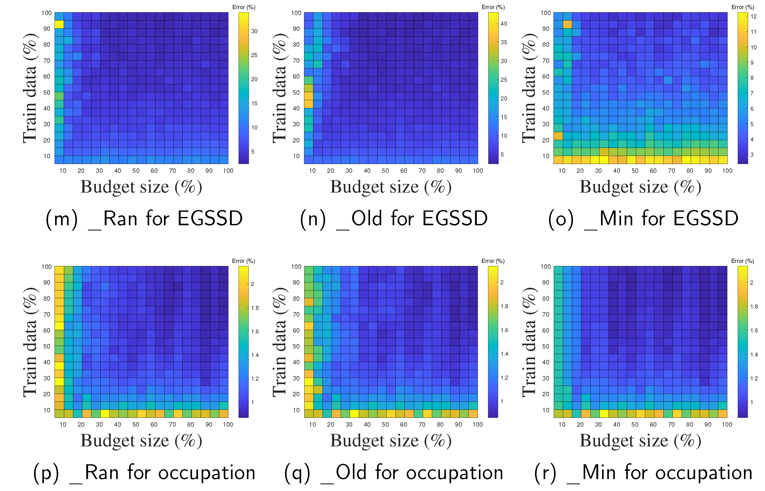
Figure 9 depicts the classification error with respect to different budget sizes as well as different amounts of training data. The error decreases with increasing the budget size percentage, and ultimately converges to the error of OSVM_SP. First, the error of the budgeted methods decreases much more quickly when the percentage is small (e.g., less than 20%), which means that a few new data points are not sufficient for learning; the performance of our proposed algorithms can thus be greatly improved by remembering more data. The rate of decrease slows when the percentage is above 40%, which implies that it is not necessary to remember all the old SVs in order to achieve comparable predictive performance. The experimental results in the above section show that when the budget size is set to one-third, the three budgeted algorithms can achieve predictive performance comparable to that of a classifier as well as a radius length comparable to that of the MEB.

6. Discussion

This paper presents OSVM_SP, a single-pass online algorithm for streaming data. Moreover, OSVM_SP-Ran, OSVM_SP-Old, and OSVM_SP-Min are proposed as three budgeted online algorithms to bound the space requirement using support vector removal principles. This section discusses the superiority and limitations of the proposed methods.

The proposed methods are superior in three distinct ways:

• OSVM_SP has the most effective predictive performance in the family of nonbudgeted online methods and is lightweight compared to batch-mode methods.
• The budgeted OSVM_SP-Ran, OSVM_SP-Old, and OSVM_SP-Min all converge steadily to the nonbudgeted OSVM_SP in their predictive performance. Compared with OSVM_SP, a decrease in the memory requirement of approximately two-thirds leads to a loss in accuracy of only about 2.0%.
• For OSVM_SP-Ran, OSVM_SP-Old, and OSVM_SP-Min, the error decreases with the increase in the budget size, and ultimately converges to the error of OSVM_SP. Moreover, the error decreases quickly/slowly when the budget size is small/large; 20–40% of the training size seems to be a proper range for the budget size.

The limitations are three-fold as well:

• Similar to the other kernelized methods, the proposed OSVM_SP has to save all of the SVs during the whole online learning process, which can become a heavy burden in restricted memory scenarios.
• OSVM_SP and its three budgeted versions are all proposed for binary classification problems. For multiple classification problems, it is possible to build a series of binary models according to one-versus-one or one-versus-rest techniques. In other words, when new samples arrive, several models have to be learned to maintain updates, which may be computationally burdensome.
• Class imbalance and missing data issues are not fully considered in this paper. Ways of adapting the proposed methods to streaming data with missing features/labels from imbalanced classes is an interesting and promising direction for future research.

7. Conclusions

In this paper, we present OSVM_SP, a new online SVM algorithm for streaming data, and three budgeted versions of OSVM_SP to bound the space requirement. All of these approaches are based on the online MEB problem and require a single pass over the streaming data. The experimental results obtained for five public datasets show that OSVM_SP outperforms most state-of-the-art single-pass online algorithms in terms of accuracy and is comparable to batch-mode SVMs and MEBs in both accuracy and radius. Our budgeted algorithms reduce the space requirement by two-thirds with only a slight loss in accuracy (0.7–5.7%).

References

- Cortes, C.; Vapnik, V. Support-vector networks. Mach. Learn. 1995, 20, 273–297. [Google Scholar] [CrossRef]
- Vapnik, V. The Nature of Statistical Learning Theory; Springer Science & Business Media: Berlin/Heidelberg, Germany, 2013. [Google Scholar]
- Wang, H.; Zhang, L.; Yao, L. Application of genetic algorithm based support vector machine in selection of new EEG rhythms for drowsiness detection. Expert Syst. Appl. 2021, 171, 114634. [Google Scholar] [CrossRef]
- Huang, C.; Zhou, J.; Chen, J.; Yang, J.; Clawson, K.; Peng, Y. A feature weighted support vector machine and artificial neural network algorithm for academic course performance prediction. Neural Comput. Appl. 2021, 1–13. [Google Scholar] [CrossRef]
- Ding, C.; Bao, T.Y.; Huang, H.L. Quantum-inspired support vector machine. IEEE Trans. Neural Netw. Learn. Syst. 2021, 1–13. [Google Scholar] [CrossRef]
- Che, Z.; Liu, B.; Xiao, Y.; Cai, H. Twin Support Vector Machines with Privileged Information. Inf. Sci. 2021, 573, 141–153. [Google Scholar] [CrossRef]
- Nguyen, H.L.; Woon, Y.K.; Ng, W.K. A survey on data stream clustering and classification. Knowl. Inf. Syst. 2015, 45, 535–569. [Google Scholar] [CrossRef]
- Lawal, I.A. Incremental SVM learning. In Learning from Data Streams in Evolving Environments; Springer: Berlin/Heidelberg, Germany, 2019; pp. 279–296. [Google Scholar]
- Guo, H.; Zhang, A.; Wang, W. An accelerator for online SVM based on the fixed-size KKT window. Eng. Appl. Artif. Intell. 2020, 92, 103637. [Google Scholar] [CrossRef]
- Mello, A.R.; Stemmer, M.R.; Koerich, A.L. Incremental and decremental fuzzy bounded twin support vector machine. Inf. Sci. 2020, 526, 20–38. [Google Scholar] [CrossRef]
- Soula, A.; Tbarki, K.; Ksantini, R.; Said, S.B.; Lachiri, Z. A novel incremental kernel nonparametric SVM model (iKN-SVM) for data classification: An application to face detection. Eng. Appl. Artif. Intell. 2020, 89, 103468. [Google Scholar] [CrossRef]
- Matsushima, S.; Vishwanathan, S.; Smola, A.J. Linear support vector machines via dual cached loops. In Proceedings of the International Conference on Knowledge Discovery and Data Mining, Beijing, China, 12–16 August 2012; pp. 177–185. [Google Scholar]
- Wang, X.; Xing, Y. An online support vector machine for the open-ended environment. Expert Syst. Appl. 2019, 120, 72–86. [Google Scholar] [CrossRef]
- Zheng, J.; Shen, F.; Fan, H.; Zhao, J. An online incremental learning support vector machine for large-scale data. Neural Comput. Appl. 2013, 22, 1023–1035. [Google Scholar] [CrossRef]
- Liu, Y.; Xu, J. One-pass online SVM with extremely small space complexity. In Proceedings of the International Conference on Pattern Recognition, Cancun, Mexico, 4–8 December 2016; IEEE: Piscataway, NJ, USA, 2016; pp. 3482–3487. [Google Scholar]
- Rai, P.; Daumé, H.; Venkatasubramanian, S. Streamed learning: One-pass SVMs. In Proceedings of the International Jont Conference on Artifical Intelligence, Hainan Island, China, 25–26 April 2009; pp. 1211–1216. [Google Scholar]
- Crammer, K.; Dekel, O.; Keshet, J.; Shalev-Shwartz, S.; Singer, Y. Online passive aggressive algorithms. J. Mach. Learn. Res. 2006, 7, 551–585. [Google Scholar]
- Ñanculef, R.; Allende, H.; Lodi, S.; Sartori, C. Two one-pass algorithms for data stream classification using approximate MEBs. In Proceedings of the International Conference on Adaptive and Natural Computing Algorithms, Ljubljana, Slovenia, 14–16 April 2011; Springer: Berlin/Heidelberg, Germany, 2011; pp. 363–372. [Google Scholar]
- Tukan, M.; Baykal, C.; Feldman, D.; Rus, D. On coresets for support vector machines. In Proceedings of the International Conference on Theory and Applications of Models of Computation, Changsha, China, 18–20 October 2020; Springer: Berlin/Heidelberg, Germany, 2020; pp. 287–299. [Google Scholar]
- Gärtner, B.; Jaggi, M. Coresets for polytope distance. In Proceedings of the Annual Symposium on Computational Geometry, Aarhus, Denmark, 8–10 June 2009; pp. 33–42. [Google Scholar]
- Chang, C.C.; Lin, C.J. Training v-support vector classifiers: Theory and algorithms. Neural Comput. 2001, 13, 2119–2147. [Google Scholar] [CrossRef]
- Kuhn, H.W.; Tucker, A.W. Nonlinear programming. In Traces and Emergence of Nonlinear Programming; Springer: Berlin/Heidelberg, Germany, 2014; pp. 247–258. [Google Scholar]
- Tax, D.M.; Duin, R.P. Support vector domain description. Pattern Recognit. Lett. 1999, 20, 1191–1199. [Google Scholar] [CrossRef]
- Tax, D.M.; Duin, R.P. Support vector data description. Mach. Learn. 2004, 54, 45–66. [Google Scholar] [CrossRef]
- Tsang, I.W.; Kwok, J.T.; Cheung, P.M.; Cristianini, N. Core vector machines: Fast SVM training on very large data sets. J. Mach. Learn. Res. 2005, 6, 363–392. [Google Scholar]
- Wang, Z.; Vucetic, S. Online passive-aggressive algorithms on a budget. In Proceedings of the International Conference on Artificial Intelligence and Statistics, Sardinia, Italy, 13–15 May 2010; pp. 908–915. [Google Scholar]
- Wang, Z.; Crammer, K.; Vucetic, S. Breaking the curse of kernelization: Budgeted stochastic gradient descent for large-scale svm training. J. Mach. Learn. Res. 2012, 13, 3103–3131. [Google Scholar]
- Wang, Z.; Djuric, N.; Crammer, K.; Vucetic, S. Trading representability for scalability: Adaptive multi-hyperplane machine for nonlinear classification. In Proceedings of the 17th ACM SIGKDD International Conference on Knowledge Discovery and Data Mining, San Diego, CA, USA, 21–24 August 2011; pp. 24–32. [Google Scholar]
- Djuric, N.; Lan, L.; Vucetic, S.; Wang, Z. Budgetedsvm: A toolbox for scalable svm approximations. J. Mach. Learn. Res. 2013, 14, 3813–3817. [Google Scholar]
- Grant, M.; Boyd, S. CVX: Matlab Software for Disciplined Convex Programming, Version 2.1; 2014. Available online: http://cvxr.com/cvx (accessed on 1 January 2022).
- Grant, M.; Boyd, S. Graph implementations for nonsmooth convex programs. In Recent Advances in Learning and Control; Springer: Berlin/Heidelberg, Germany, 2008; pp. 95–110. [Google Scholar]
- Zhao, P.; Zhang, Y.; Wu, M.; Hoi, S.C.; Tan, M.; Huang, J. Adaptive cost-sensitive online classification. IEEE Trans. Knowl. Data Eng. 2018, 31, 214–228. [Google Scholar] [CrossRef]
- Sahoo, D.; Pham, Q.; Lu, J.; Hoi, S.C. Online Deep Learning: Learning Deep Neural Networks on the Fly. In Proceedings of the IJCAI, Stockholm, Sweden, 13–19 July 2018. [Google Scholar]
- Gözüaçık, Ö.; Can, F. Concept learning using one-class classifiers for implicit drift detection in evolving data streams. Artif. Intell. Rev. 2021, 54, 3725–3747. [Google Scholar] [CrossRef]
- Din, S.U.; Shao, J.; Kumar, J.; Mawuli, C.B.; Mahmud, S.; Zhang, W.; Yang, Q. Data stream classification with novel class detection: A review, comparison and challenges. Knowl. Inf. Syst. 2021, 63, 2231–2276. [Google Scholar] [CrossRef]