
Sampling Rate Optimization and Execution Time Analysis for Two-Degrees-of-Freedom Control Systems †


Department of Automation, Technical University of Cluj-Napoca, Str. G. Bariţiu nr. 26-28, 400027 Cluj-Napoca, Romania
*
Authors to whom correspondence should be addressed.
†
This paper is an extended version of our paper published in 2022 IEEE International Conference on Automation, Quality and Testing, Robotics (AQTR), Cluj-Napoca, Romania, 19–21 May 2022. https://0-doi-org.brum.beds.ac.uk/10.1109/AQTR55203.2022.9802027 .
‡
These authors contributed equally to this work.
Mathematics 2022, 10(19), 3449; https://0-doi-org.brum.beds.ac.uk/10.3390/math10193449
Submission received: 25 August 2022
/
Revised: 13 September 2022
/
Accepted: 16 September 2022
/
Published: 22 September 2022
(This article belongs to the Section Engineering Mathematics)
Abstract
:The current journal paper proposes an end-to-end analysis for the numerical implementation of a two-degrees-of-freedom (2DOF) control structure, starting from the sampling rate selection mechanism via a quasi-optimal manner, along with the estimation of the worst-case execution time (WCET) for the specified controller. For the sampling rate selection, the classical Shannon–Nyquist sampling theorem is replaced by an optimization problem that encompasses the trade-off between the fidelity of the controllers’ representation, along with the fidelity of the resulting closed-loop systems, and the implementation difficulty of the controllers. Additionally, the WCET analysis can be seen as a verification step before automatic code generation, a computational model being provided. The proposed computational model encompasses infinite-impulse response (IIR) and finite-impulse response (FIR) filter models for the controller implementation, along with additional relevant phenomena being discussed, such as saturation, signal scaling and anti-windup techniques. All proposed results will be illustrated on a DC motor benchmark control problem.
Keywords:
sampling rate; closed-loop cascade control; discrete-time systems; global optimization; rapid control prototyping; worst-case execution time; IIR filtering; FIR filteringMSC:
93C05; 93C57; 93C621. Introduction
1.1. Literature Review
The problem of sampling rate choice to numerically implement a controller designed in the continuous-time domain has significant importance. A sub-optimal value of the sampling period represents a trade-off between the fidelity of the response, given by a shorter sampling rate, and implementability, obtained using a larger sampling rate. The most common manner to choose this sampling period is given by the Shannon sampling theorem [1]. However, this can only be a starting point in a control context, because, in practice, it can lead to unacceptable behavior of the discrete-time controller compared to its continuous-time equivalent, a significant justification being the presence of quantization errors unaccounted for in the signal and system models. In the available literature, the problem of choosing the sampling rate is specifically formulated for the purpose of the particular control system at hand. For example, for a structure with a P-type regulator proposed in [2], the key points used in sampling rate selection are the overshoot and the rise time. For the case of a PID-based control structure, an optimization criterion has been proposed in [3] to find the optimal and/or sub-optimal value of the sampling rate. The problem of sampling rate selection for parameter estimation of an induction machine has been solved via a metaheuristic procedure in [4]. A similar thematic is addressed in [5] in the case of permanent magnet synchronous motors using field programmable gate array devices, while the rapid control prototyping principle is illustrated for discrete-time closed-loop control of brushless DC motors in [6,7], respectively. Moreover, an important result regarding the dependence between the stability and the performance of the closed-loop system, and the choice of sampling rate is presented in [8].
After the first step of selecting the sampling period, an analysis regarding the practical implementation of the proposed control structure on a microprocessor-based system should be performed. This analysis needs to encompass several aspects which are not explicitly modeled in the control law, such as the register word lengths of the coefficients which directly influence the number of necessary assembly instructions, and saturation, overflow, underflow verifications on the computed command signals. In the specific context of rapid control prototyping (RCP), one key step before the proper code generation is to certify if its execution abides by the time span given by the sampling period. Moreover, other important verifications for phenomena such as underflow and overflow, or saturation and anti-windup techniques should be also performed before the code-generation step. As such, one important goal consists of approximating the number of software operations necessary to implement the designed control law, mandatory in the context of hard real-time systems. A survey of worst-case execution time computational methods is presented in the seminal paper [9]. A simplified study applied for control system-related interrupt service routines for state-space controller representations is presented in [10]. Another possibility for the computational error analysis is presented in [11].
In the Control Systems domain, the linear control system field plays an important role. Linear controller design techniques are available for both linear plants and nonlinear process models alike. Starting from the classical proportional–integral–derivative (PID) controller [12] towards the domain of robust controller [13,14,15], these techniques can be extended for nonlinear systems via the gain-scheduling method [16] or an additional passivity-based component [17]. Moreover, with great advantage in also coping with disturbance rejection problems, alongside reference tracking specifications are the so-called two-degrees-of-freedom (2DOF) control schemes [13]. In ref. [18], a 2DOF PID controller has been proposed, where the serial compensator is a classical PID controller, while the feedforward compensator is a PD controller, the integral effect being excluded due to the stability requirements. For the case of unstable plants with time delays, a discrete-time 2DOF control scheme has been proposed in [19]. As such, for reference tracking, the serial controller was designed using the optimal control framework, while the feedforward controller has been tuned by imposing the desired closed-loop transfer function. Additionally, in terms of software toolbox implementations, the robust advanced PID (RaPID) toolbox described in [20] presents a set of possibilities to design a 2DOF PID control structure by minimizing certain error criteria, such as the integral of absolute error or integral of time multiplied by the absolute value of error.
1.2. Contributions and Paper Structure
The current journal paper represents an extension of the conference papers [10,21], and proposes a joint analysis on sampling time selection and execution time framing of the microcontroller operations into the previously established optimum for the case of a 2DOF control structure. The main contributions of the paper are:
- (i)
- to extend the functionals initially proposed in [21] in order to encompass the fidelity of both controllers from the 2DOF structure and of the resulting closed-loop systems, i.e., ensuring the tracking and servo behavior of the initially designed continuous-time controllers, along with the implementation difficulty of the proposed controllers in terms of quantization and sampling rate span;
- (ii)
- to formulate the optimization problem for sampling rate selection of a 2DOF control structure without considering any further normalizations of the final functional’s terms and propose a metaheuristic-based solution to find an optimal or quasi-optimal value of the sampling rate which can offer a good trade-off between implementability and fidelity;
- (iii)
- to extend the WCET analysis, initially proposed in [10] for the case of state-space regulator implementations, for the case of controllers implemented as infinite-impulse response (IIR) or finite-impulse response (FIR) filters, offering an upper bound estimation of the time span necessary to perform all the operations involved in the numerical implementation of the proposed 2DOF controller;
- (iv)
- to offer an exhaustive analysis which can be further performed in an automatic manner and to be integrated in our open-source MATLAB-based CACSD toolbox [22];
- (v)
- to present an end-to-end design procedure for the case of a DC motor control problem, starting from the controller design, followed by choice of the quasi-optimal sampling rate and the worst-case execution time analysis, finalizing with a detailed discussion.
The rest of the paper is organized as follows: Section 2 presents the 2DOF structure which will be studied, along with a mathematical background for the sampling rate choice and worst-case execution time analysis, and a set of theoretical results and optimization problems extended and adapted for the proposed control structure; in Section 3 a case study consisting of an end-to-end design procedure of a 2DOF PID controller is illustrated, while Section 4 deals with a set of conclusions and further research directions.
1.3. Notations
We denote by the circle with the center in and radius . Additionally, and denote the pole and zero sets of an LTI system G, respectively. An arbitrary sampling period will be denoted throughout the paper. Continuous-time regulators will be denoted , while their discrete counterparts, as a function of the sampling period will be used as . The set of continuous-time systems will be denoted by , while the set of discrete-time systems will be denoted by . The standard growth functions and their notations according to [23]:
2. Mathematical Background and Proposed Extensions
2.1. Numerical Closed-Loop Control
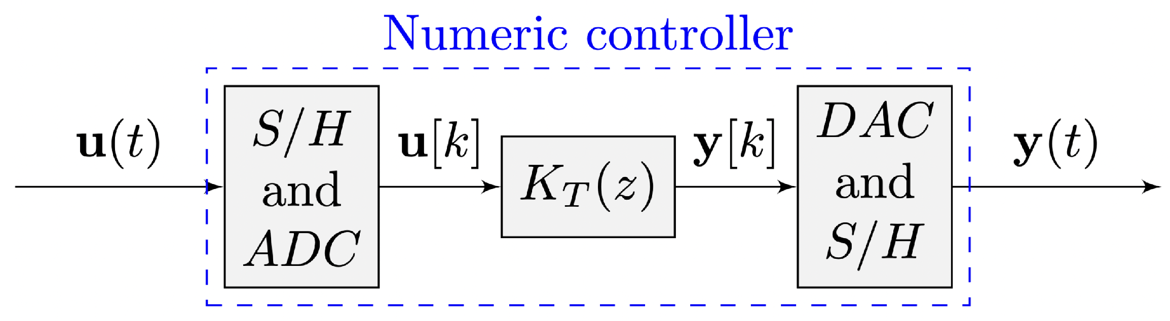
Modern control systems make use of numerically implemented regulators to coordinate continuous-time processes. The classical configuration of a numerical regulator is presented in Figure 1. It uses sample and hold circuits as interfaces to the continuous-time adjacent components and, as such, it imposes the zero-order hold discretization method for the plant G. As such, define the plant discretization methodology as the mapping :
with denoting the continuous-time model set, being the discrete-time model set, and with the digital-to-analog converter, i.e., zero-order hold, model:
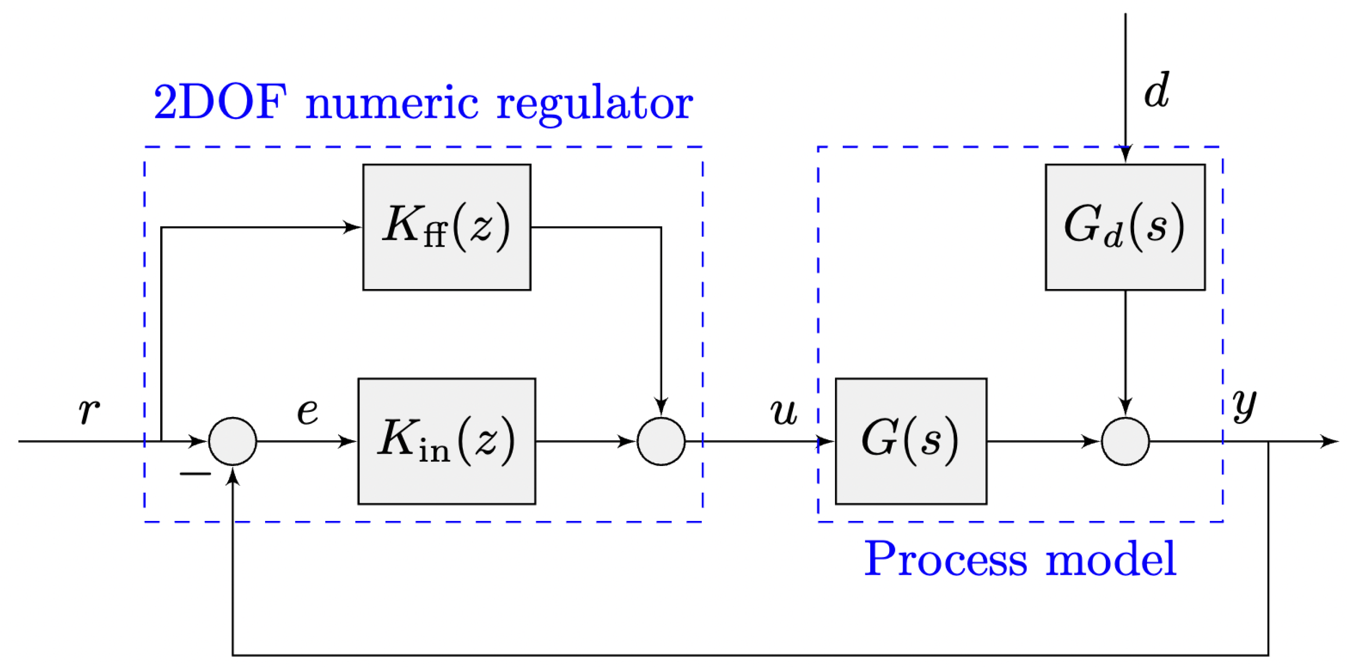
For the purpose of this paper, we consider a two-degrees-of-freedom (2DOF) control structure as in Figure 2, which has an inner controller usually designed for disturbance rejection, and a feedforward controller which provides the necessary compensation for the steady-state tracking behavior, along with the process model with disturbance, described by and . As does not influence the signal path from the disturbance to the output , the usual design workflow is to synthesize and, then, to fine-tune the transient response from to through . Both continuous-time controllers and are assumed to have the following linear and time-invariant (LTI) state-space representations:
Given that the continuous-time controllers and must be numerically implemented on a microcontroller, the problem of selecting an appropriate sampling period becomes a critical step. For a fixed sampling rate T, the discrete-time form of a controller can be written as:
To compute the transition matrix and the input matrix , a wide selection of discretization methods, denoted by , can be considered, such as zero-order hold, trapezoidal (Tustin), forward or backward Euler, frequency-response regression and so on. Additionally, in most situations, the output matrix remains the same as in the continuous-time representation, but there exist cases when it may be different than its continuous-time counterpart. As such, from a tuple of a continuous-time transfer matrix and a sampling rate results an equivalent discrete-time transfer matrix , where:
The open-loop process model has the input-output representation:
while the closed-loop system expression becomes:
The discrete-time equivalent closed-loop model will be:
which represents the starting point for various control design methodologies.
2.2. Sampling Rate Optimization
The current subsection presents an extension of the work from the paper [21].
2.2.1. Linear System Sampling Background
The well-known Shannon theorem [1] states that the necessary sampling rate to avoid information loss must be at most twice time smaller than the inverse of the continuous-time signal’s maximum frequency component:
Moreover, the theoretical upper bound of the frequency range after which aliasing phenomena occur is called Nyquist frequency and is given by:
The above-mentioned version of Nyquist-Shannon theorem for signals can be extended to LTI systems by considering that the resulting discrete-time system must maintain all relevant dynamics of the continuous-time system. The dynamics of a system is given by its set of poles, one possible constraint for the sampling rate implying to be at most twice smaller than the inverse of the real part of the minimum value of poles. However, there are cases when the imaginary part of the poles is relevant, or even the values of the transmission zeros, for a good representation of the system’s frequency response.
For the remainder of the paper, the sampling rate will be denoted by . The analytical relationship between the continuous-time s-plane and the discrete-time z-plane is illustrated by the equation:
Considering a point , with , the resulting corresponding complex number is . As such, the left half of the complex s-plane can be split into an infinite number of disjoint strips of height , due to the periodical nature of the and functions. The resulting primary strip contains points which correspond to . The s-plane to z-plane mapping causes the following topologies of the primary strip of the s-plane:
- the imaginary axis in is mapped to the unit circle ;
- the upper and the lower edges are both mapped to the negative axis;
- the negative real axis is mapped to the positive axis inside the unit circle;
- the interior of the primary strip is mapped in the unit disk.
When sampling an LTI controller, several remarks can be considered then the behavior of the singularities is studied:
- (i)
- unstable zeros and poles tend decreasingly to the unit circle’s circumference, i.e., and as ; for poles, this aspect is relevant when sampling systems, as controllers generally do not employ unstable poles in their structure;
- (ii)
- stable zeros and poles tend increasingly to the unit circle’s circumference, i.e., and as , requiring additional decimal or binary digits for an accurate representation.
- (iii)
- poles and zeros from the imaginary axis in the s-domain are maintained on the unit circle in the z-domain irrespective of the sampling period . Additionally, integrator and derivative terms do not matter in deciding the practical sampling time.
- (iv)
- the quantization error increases as in the case of stable closed-loop systems.
Remark 1.
The quantization error mentioned in (iv) increases as as proved in [24], due to the guaranteed steady-state error being proportional to , while denotes the spectral radius of the closed-loop state matrix: , based on the series interconnection between the controller and the process model matrices.
According to the previously mentioned aspects, a sub-optimal value of the sampling rate must ensure a good trade-off between the fidelity of the representation of the continuous-time controllers and their implementability difficulty. As such, we next introduce a set of functionals to quantify these two aspects.
2.2.2. Proposed Functionals
To measure the similarity between a continuous-time LTI system and a discrete-time system over the frequency range , the following functional can be defined as , with :
where is the maximum singular value. Moreover, as mentioned before, the available frequency domain is , being the corresponding Nyquist-Shannon frequency to the sampling rate T. Therefore, the similarity functional becomes:
However, to compute the similarity integral term , a discrete set from the frequency range can be considered, the performance index being approximated as follows:
where is a predefined threshold used to avoid the prewarping phenomenon which ensues in the magnitude responses when .
Remark 2.
There are several alternatives in defining the similarity between two LTI systems, with particular interest for closed-loop connections, such as the normalized dissimilarity function metric, described in [25], the standard ν-gap metric, with its limitations exposed in [26], or the improved Vinnicombe ν-gap metric [27], described as:
with:
where for the reference systems and , their right normalized coprime factorizations will be considered: and , which in context of the proposed sampling rate optimization problem, the differences should be computed with the subsystems applied in and , respectively.
To define the fixed-point implementability functional which measures the quantization implementation difficulty of the LTI system , the following expression can be considered:
with and denoting the pole and zero sets of , respectively, excluding singularities from the set .
Alongside the previous implementability functional, an execution time cost functional becomes necessary to limit the decrease of which would ideally lead the similarity functional costs to zero:
A concluding functional with global effect, , will define the feasibility domain of the optimization problem, because it accepts or rejects a specific sampling period value. It induces an infinitely valued constant when the numeric system becomes unstable, and otherwise, defaults to no extra penalization:
For the numerical implementation of the stability functional, a sufficiently large value can be considered to mark the feasibility subdomain of where the system H is stable, leading to an approximation of the original performance index:
2.2.3. Optimization Problem
For the two-degrees-of-freedom control structure proposed in Figure 2 the following functionals will be considered to formulate the optimization problem to determine the sampling rate:
- two terms and representing the similarity between the continuous-time and the discrete-time representations of the controllers and over the frequency range ;
- two terms and representing the similarity between the continuous-time and the discrete-time representations of the resulting closed-loop systems and over the same frequency range;
- the quantization implementation difficulty and of each controller along with the execution time functional ;
- the stability functional of the resulting numerical closed-loop system .
The first set of three terms are used to measure the fidelity between the components of the continuous-time designed system and the resulting components in the discrete-time domain, considering the transient and steady-state performance altering. The next set of three terms manages to encompass the implementation difficulty of the resulting controller, according to the already-mentioned remarks. The last term is nothing but a correction used to define the feasibility subdomain of . As such, a trade-off between the first two sets of performance indices must be established by taking into account the last feasibility term, resulting a non-convex optimization problem. However, in order to increase the flexibility of this optimization problem, a set of weights can be considered as follows: the weights , , , and are for the fidelity measurement indices, while weights , , and are for the implementability indices, the final functional being:
Moreover, considering the numerical approximations (14) and (20), the following numerically implementable non-convex optimization problem occurs:
Problem 1.
For an LTI plant model included in a two-degrees-of-freedom control structure with the continuous-time inner controller and with the continuous-time feedforward controller as in Figure 2, define an ordered set of pulsations, preferably in logarithmic scale:
Then, the functional :
with weighting terms , leads to the following quasi-optimal sampling time optimization problem:
Remark 3.
The resulting optimization problem (24) is non-convex by nature. As such, the line-search procedure used to solve this problem must be able to explore the whole feasible domain. One possible solution is a metaheurisitc approach, such as particle swarm optimization (PSO) [28], which will be used for the purpose of this paper.
2.3. Worst-Case Execution Time Analysis
The current subsection presents an extension of the work from the paper [10].
2.3.1. Execution Time Model
This subsection proposes the study of the implementation details for the case of linear control structures, where controllers will be modeled as infinite-impulse response (IIR) and finite-impulse response (FIR) filters. Starting from [10], a set of implementation aspects which are treated for state-space realizations will be considered in a unified manner for the case of transfer matrices in this paper. Additionally, this section also analyzes the 2DOF extension. The duration for each operation involved in the control structure can significantly impact the regulator implementability.
The necessary mathematical operations to fully implement an LTI-based control law must be formally defined. Besides the LTI-control law, the classical saturation and anti-windup nonlinearities will be considered, which are usually related to said LTI laws. The unary and binary mathematical operators defined in Table 1 and gathered in the operations alphabet , are considered with real operands and must be accounted for into a microprocessor-based environment.
As such, the process of computing a command signal as in Figure 1 implies a finite and formal computational finite sequence , where all terms are mathematical operations as in Table 1, i.e., , , where N depends on the structure of the controller . Moreover, in order to additionally specify a set of practical hardware specifications and constraints and to uniformly describe the problem, the finite sequence can be now extended to a full sequence :
Starting from an array of operations as (25), we follow with a general-purpose instruction set model. Assume a Random-Access Machine (RAM) computational model as in [23], with deterministic operations. RAM machines have practical counterparts, materialized through RISC machines. Reconfigurable RISC machines specialized on certain problems have been proposed in [31]. Additionally, there is the approach of multiply and accumulate (MAC) instructions supported in digital signal processors (DSP) [32]. Depending on the supported computer architectures of the RCP framework, relevant are also Single Instruction stream/Multiple instruction Pipelining (SIMP) [33] constructions with respect to single-processor architectures, or Single Instruction/Multiple Data (SIMD) features, which allow the practical parallelization of addition and multiplication operations for several sets of operands.
Definition 1.
The hardware constraints and specification set encompasses metadata which imply extra operations or different approaches to the standard operations performed on the controller signals and implementation-specific information, with various outcomes on the total execution time, frequently found in practice being:
- reading reference signals and plant measurements , all input signal reading steps may imply preprocessing constraints in terms of sensor delays, impulse counters or data type conversions—this equates to adding steps;
- scaling operations for the input and output signals imposed by the operating point used for plant linearization: and , which equates to augmenting the sequence set with items;
- input and output signals scaling operations, i.e., and , useful especially for sensor/adapter signals, and extend the operations with ;
- starting from the variable base word length L of the microcontroller arithmetic registers which allows operations to be executed in a single clock tick, each variable’s type and size should be adequately adapted for , etc., which complicates the adding and multiplication routines with additional steps;
- controller gain-scheduling verifications and updates based on the value of the input signal , leading to extra ;
- underflow and overflow checks for involved signals, implying saturations ;
- availability of Direct Memory Access (DMA) modules, MAC instructions, circular buffers in opposition to linear buffering, or output bypassing, which has the advantage of discarding operations.
Such specifications will be quantified by scaling factors to the base duration of the RISC machine model operations. Depending on the significance of the alternative instruction, could be less than, equal to, or greater than one, respectively.
Therefore, a set of instructions can be manually designed or automatically deduced. For manual modeling, the control engineer needs to find this set for each control law, while for automatic mode, an RCP tool can already deduce this set. Such an RCP tool generally deals with the code generation for different environments. Now, the sequence of operations generator procedures can be seen as a functional:
To implement the mathematical operations from Table 1, the atomic assembly instructions from Table 2 will represent the starting point. It covers the basic arithmetical operations required in linear systems, with the additivity and homogeneity properties, conditional jumps for saturations and the anti-windup of integrator terms, forced and imposed delays through data acquisition hardware and access to memory devices. Each arbitrary atomic assembly operation will be denoted by a, as part of the formal set all the equivalent assembly instructions supported by for the implementation of , with the RISC machine assumption that each instruction takes a fixed clock tick value > 0. The number of ways in obtaining the resulting assembly instructions is not unique and it further depends on the structure of . A straightforward example to illustrate this phenomenon is when the regulator coefficients are stored contiguously in the memory in comparison to arbitrary and uncorrelated memory registers. The execution time implications are obtained through different pointer operations. To conclude, a new mathematical operator analogous to (26), tasked with the generation of a computer-equivalent set of instructions given by the functional is:
which results in an infinite sequence of atomic software instructions, but with a finite number of them being different to NOP, located at the start of the sequence, which implement the linear controller formula:
The difference between the sets and is that contains abstract mathematical operations , and each such operation will be practically implemented using equivalent steps, , as in the mapping:
the number of atomic operations different from NOP being .
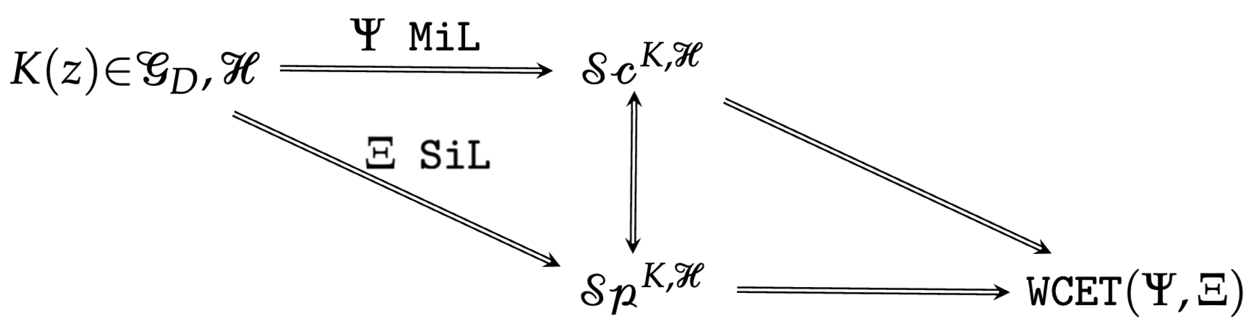
The importance of the previously defined sequences and functionals, i.e., , , and , respectively, and the implications of estimating the number of assembly operations in a tight manner was insisted upon in the base paper [10]. Figure 3 gathers them and illustrates their connections in an RCP context. The mapping from to the set is usually performed for Model-in-the-Loop (MiL) simulations through an application , while the mapping is made through Software-in-the-Loop (SiL) testing using an application . The master RCP program, with access to both and , can subsequently perform a worst-case execution time analysis on the implementation of the digital regulator in the production hardware context .
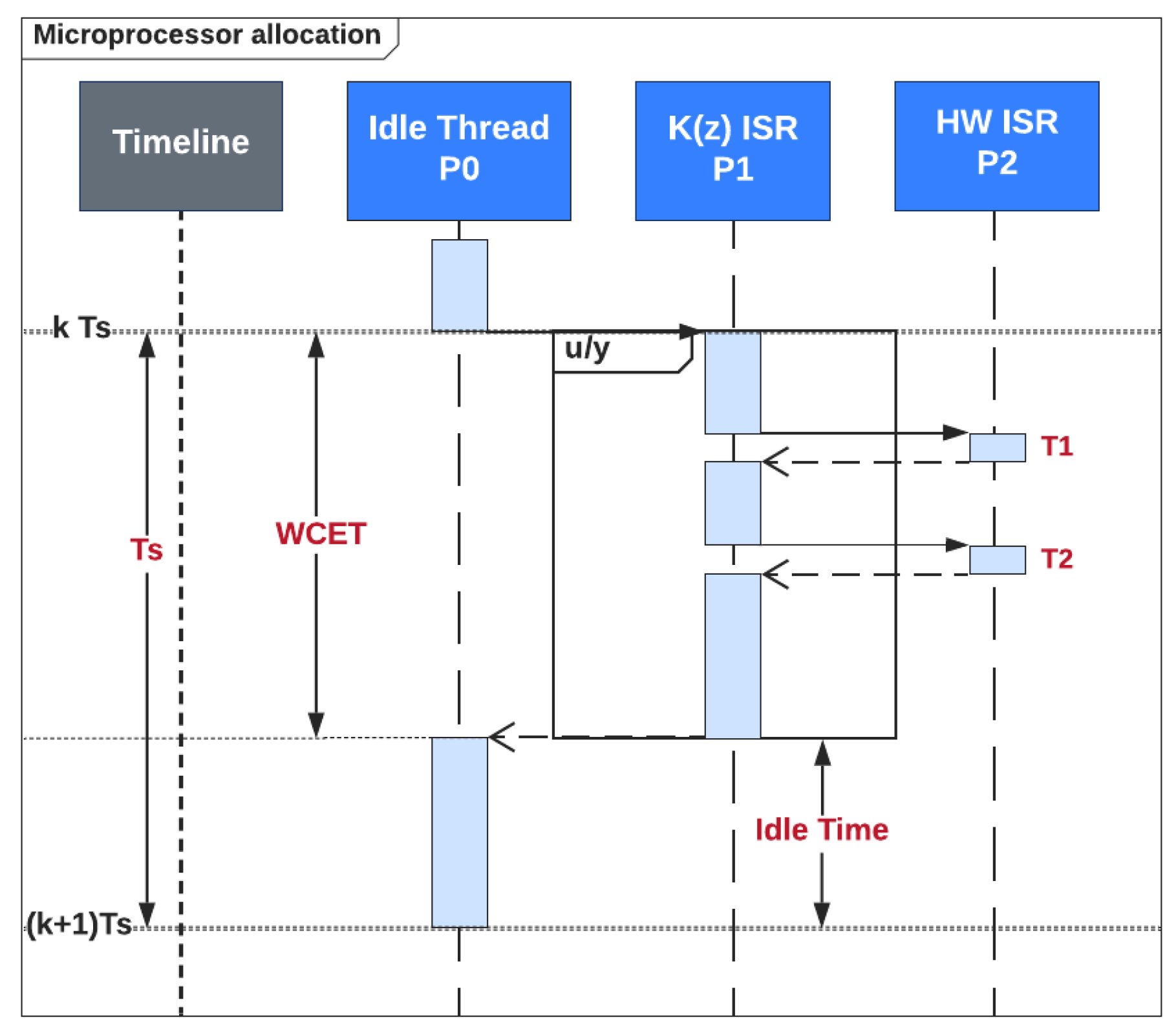
Figure 4 presents the sequence diagram with the timing constraints of the discrete-time controller K with respect to other software threads from the microcontroller, with an illustration of the WCET of the controller interrupt service routine (ISR) thread. The main result of the section is gathered in the following theorem.
Theorem 1.
Given a numerical control law given by , along with a microcontroller specification set and a code-generation procedure given by a pair of MiL and SiL , the worst-case execution time estimation can be computed by the following formula:
where represents the number of atomic assembly operations as in (28), and accounts the context switching operations for the other software threads. Additionally, the exact bounds from depend on all other software entities running on the same microprocessor and are not correlated with the input dimension m or the output dimension p of the numerical controller.
Proof.
According to the schematic representation from Figure 3, starting from the control law and the specification set , the set can be obtained via the MiL operator , resulting in . However, in order to measure each , the set of atomic operations must be attached via the SiL operator : , each such atomic operation requiring exactly , leading to:
where is the time necessary to execute an operation or a set of operations.
Additionally, a second term accumulates ISR switching and stack-handling operations handled by the scheduler, bounded by a processor-dependent constant , which can be modeled as . As such, the worst-case execution time can now be written as:
which concludes the proof. □
Observation 1.
All possible delays caused by context switching to preemptive ISRs belonging to measurement data processing, with the cost of , are included in the input processing step and do not remain unaccounted for in the execution time model of Theorem (30).
Two additional performance qualifiers can be employed to globally assess the controller ISR implementation impact on the scheduling algorithm of the processor.
Definition 2.
The processor usage level qualifier relative to a fixed sampling period of a discrete-time regulator , described in a relative manner, is defined by:
Definition 3.
The processor idle time qualifier with respect to a fixed sampling period of a discrete-time regulator , described in absolute units, is defined by:
2.3.2. Modeling Duration of Finite and Infinite-Impulse Response Topologies
Denote by a MIMO regulator with m inputs and p outputs, thus fully described by the expressions of transfer functions :
Each element of the transfer matrix , i.e., , can be modeled as an infinite-impulse response (IIR) filter or as a finite-impulse response (FIR) filter. The case where is modeled as a state-space representation is treated in the base conference paper [10], namely in Algorithm 1 and Table I, respectively.
For an arbitrary discrete-time IIR transfer function of order n, define as the pair:
Using this notation, the transfer function can be written using a series of second-order sections and an additional first-order component, if necessary, as:
with the terms from each triplet not all null, known as a first-order section, and each , with being denoted in the literature as a second-order section (SOS).
Remark 4.
Second-order sections are usually described with an additional gain term multiplied separately to the output of the transfer function as:
To not further complicate the notations, we will not explicitly write this gain term for every second-order section, but it will be implicitly considered in the implementation and execution time analysis.
There are multiple approaches of implementing digital biquadratic filters, a good example being the description from the monograph [34]. Table 3 exposes the four usual topologies, which principally implement the same input-output transfer function, but with important differences regarding numerical stability when selecting fixed-point or floating-point implementations. These configurations are referred to as the canonical forms: Direct Form I, Direct Form II, Transposed Form I, Transposed Form II, which differ in the numerical properties of their implementations and in the number of necessary delay elements. As observed in the third column of the table, all biquad topologies are based on four additions, five multiplications, and a different number of load/store operations, depending on the definition of the internal state variables. Such implementation details are relevant when studying particularized structures, such as in the situations treated in [35,36].
The ISR model for IIR controller structures is based on the pseudocode exposed in Algorithm 1. hlBased on the specifications for , each line of the pseudocode will have a set of mandatory mathematical operations, along with optional operations, which will be accounted for in the execution time analysis model through different constant weights.
| Algorithm 1 Infinite-impulse response (IIR) filter interrupt service routine (ISR) |
|
In ref. [10], an analysis has been performed on the simplified case of a nth order IIR SISO transfer function in a series connection, described as:
which, by design, it can implicitly include a delay by forcing the first coefficients to zero. Such a transfer function has its corresponding difference equation as:
A further particularization on the structure of is to consider the expression of a FIR filter topology, which, by design, discards the previous output delays. The present command signal will, as such, depend only on an array of delays, i.e., delay tap of inputs , modeled as:
Four typical canonical forms are distinguished for FIR-type filters, namely the Direct Form (DF), Direct Form Transposed (DFT), Symmetric and Antisymmetric [34], respectively, with their definitions exposed in Table 4. The main difference between DF and DFT is that for the former, the delay word lengths are that of the input signals , while for the latter, the delays have the word length of the accumulator variable. The Symmetric and Antisymmetric cases make use of the linear phase of the filter through the regularity of the first coefficients as the symmetrical or antisymmetrical equivalents of the latter half of the coefficients. As mentioned in the third column of the table, this has a significant impact on the necessary multiplications and load operations involved in the implementation of . Algorithm 2 emphasizes the corresponding SISO FIR filter ISR routine starting from the mathematical basis of Equation (41) and information from Table 4.
Corollary 1.
Given a MIMO transfer matrix as in (35), where each component , can be described as an IIR filter of form (37), with second-order sections as in Table 3 or a FIR filter of form (41), with difference equations as in Table 4, the WCET can be computed as:
with coefficients accounting for the hardware specifications set from Definition 1, each assembly operation set determined individually by the RCP application, given the microprocessor tick , and depends only on the other higher-priority software threads.
| Algorithm 2 Finite-impulse response (FIR) filter interrupt service routine (ISR) |
|
The proof immediately follows based on Theorem 1 by replacing the general-purpose sequence with its corresponding sum of subsystems from the full MIMO regulator and their definitions.
3. Case Study
The Case Study section concerns with illustrating the proposed extensions on a motor servo control example, and will encompass the following key points: process description, control performance specifications, continuous-time controller design, regulator discretization methods, sampling time optimization, selection of different controller implementation topologies along with the worst-case execution time analysis and a detailed discussion of the obtained results. The reason for selecting this example is that the proposed theory can be illustrated in the same manner for a simple process model and a modest microcontroller device setup, compared to a more complex process and an adequate microcontroller setup, leading to similar processor workloads.
3.1. Process Model and Controller Synthesis
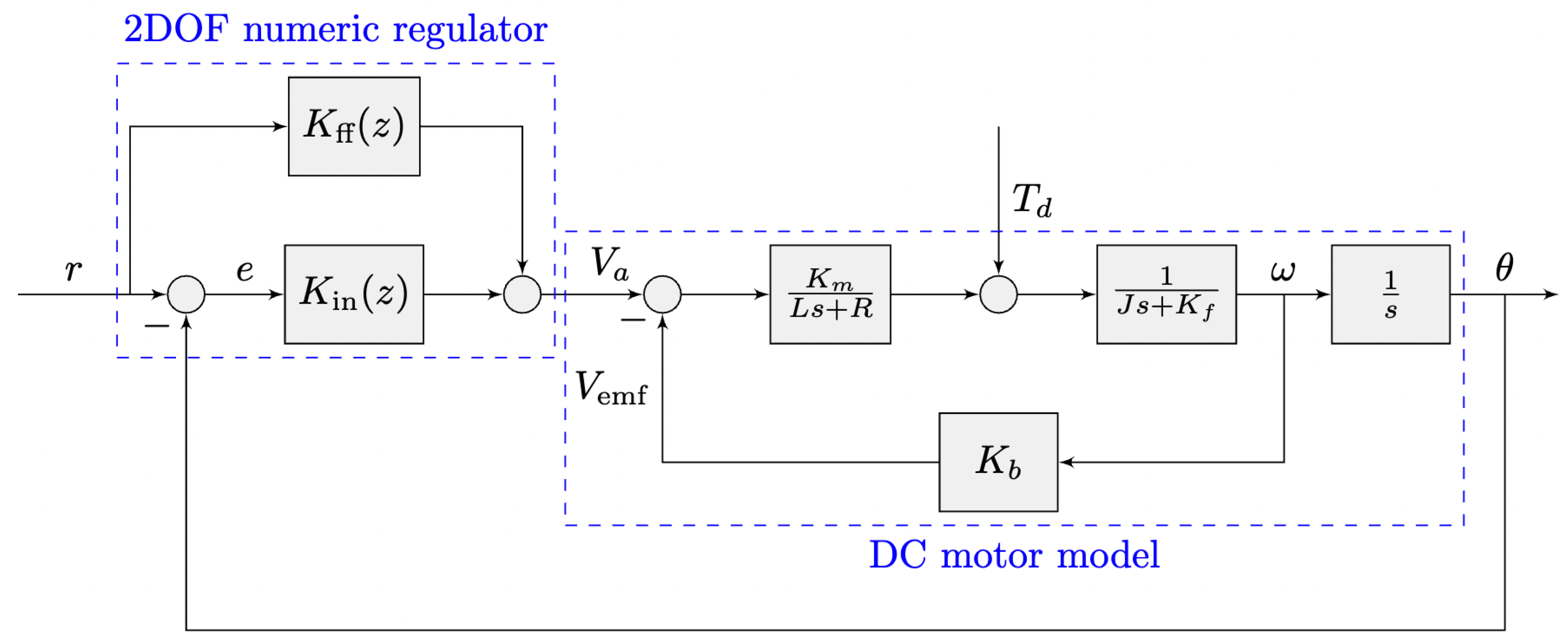
To illustrate the proposed theoretical techniques, we consider a numerical case study based on a brushed direct-current (DC) motor position control system. Figure 5 shows the closed-loop structure, emphasizing both the process model and the 2DOF regulator structure. The motor process has a control input represented by the source voltage [V], along with the disturbance load torque [Nm], and the output is considered to be the angular position [rad]. As noticeable from the transfer function blocks, the DC motor model has order three, and the nominal component values are listed in Table 5.
The process model from its two inputs to the angular position output is described by:
with the armature transfer function , along with the load component and the reverse loop term which denotes the back-electromotive voltage constant :
The 2DOF controller components have the proportional–integral–derivative plus filter (PIDF) structure for , while the integral term is canceled for the feedforward controller . This structure allows straightforward implementation in many industrial contexts as such PIDF regulators can be directly acquired and there are multiple validated approaches in the literature for their parameter tuning [18,20]. As such, their mathematical expressions become:
with the feedforward parameters usually specified as b and c, with and . The command signal applicable to the motor input is comprised of two components derived from the 2DOF regulator as:
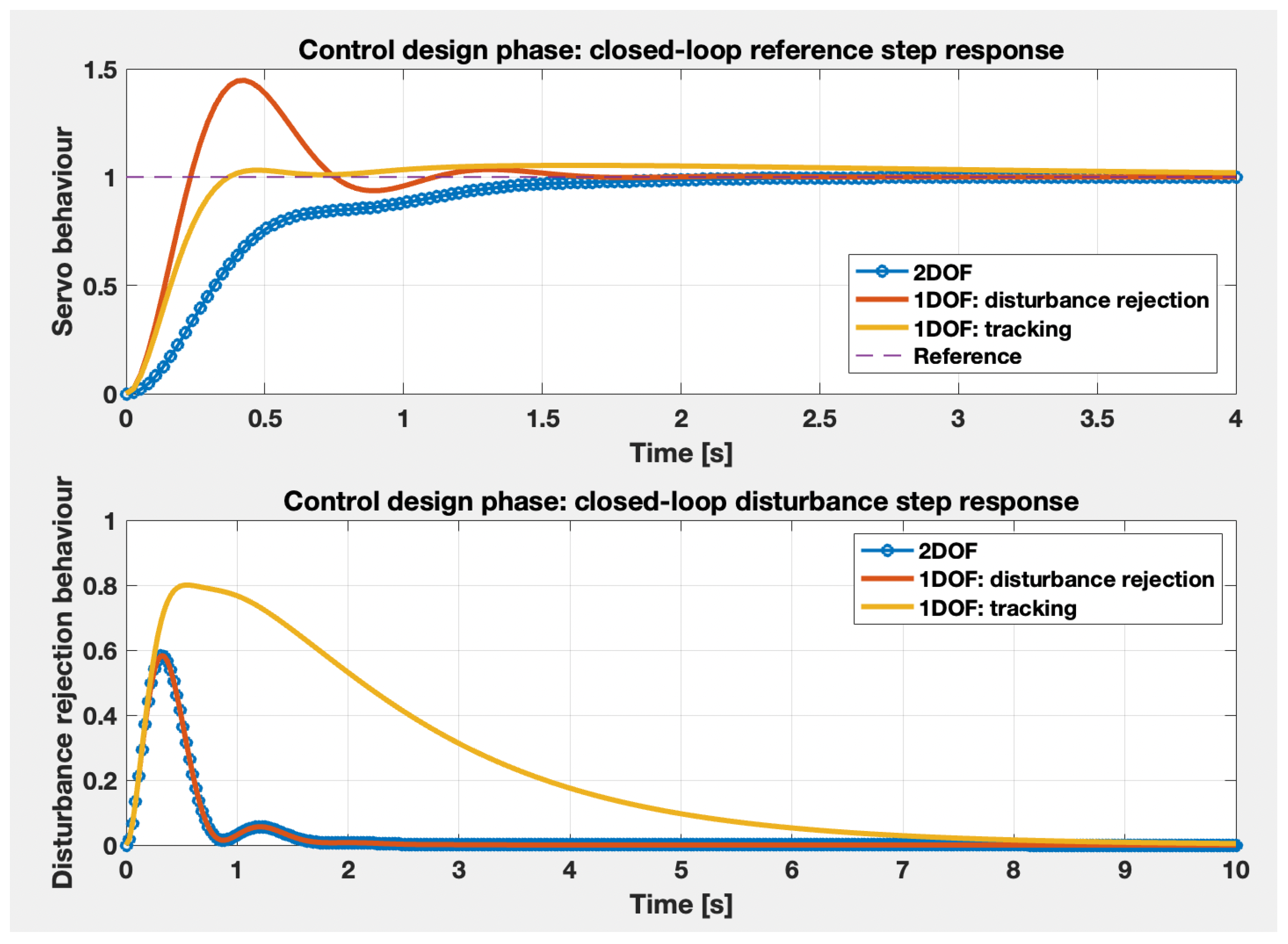
The closed-loop control specifications were selected as follows: a reference tracking settling time of [s] with an overshoot [%], with the rise time as short as possible. Additionally, regarding the disturbance rejection specifications, a load torque of 1 [Nm] must be rejected in less than [s], i.e., its effect on the output measurement should become less than [rad] in the specified , with a maximum allowed disturbance of [rad]. The recommended approach in such designs [12] is to tune the inner PIDF controller to account for the disturbance rejection coefficients, as does not influence that control loop, as written in the discrete-time counterpart expressions (54). The PIDF parameter tuning has been done using global optimization methods by encompassing the desired specifications. The first iteration which covered all disturbance rejection performances was accepted and halted the optimization procedure. Additionally, a further optimization as been performed on the 2DOF parameters b and c of (46) with, again, halting the procedure after the reference tracking requirements have been fulfilled. The outcomes of the regulator tuning are illustrated in Table 6, where, alongside the PIDF and additional PD synthesis, a separate 1DOF PIDF regulator has been also added, to account for only the tracking response.
The closed-loop step responses for the reference tracking and disturbance rejection problems are portrayed in Figure 6, showing the effects of the three controller examples from Table 6, case in which the 2DOF structure is validated, as the obtained performance metrics are [s], , rise time [s] and steady-state error . As illustrated in the figure, the 2DOF structure manages to ensure both the transient response performances and the disturbance rejection behavior, being the only regulator from the proposed triplet to cover both areas.
3.2. Sampling Rate Selection
For the discretization of the PID regulators, the forward Euler method has been considered for the integrator term, with the approximation:
while the derivative term is discretized using the backward Euler method as:
leading to the expression of :
with an expression of also as:
which will be further used in the proceeding illustration of the sampling time analysis.
Starting from the continuous-time open-loop model from (43), the discrete-time equivalent using the zero-order hold method becomes:
with the auxiliary notations:
The closed-loop system’s expression thus becomes:
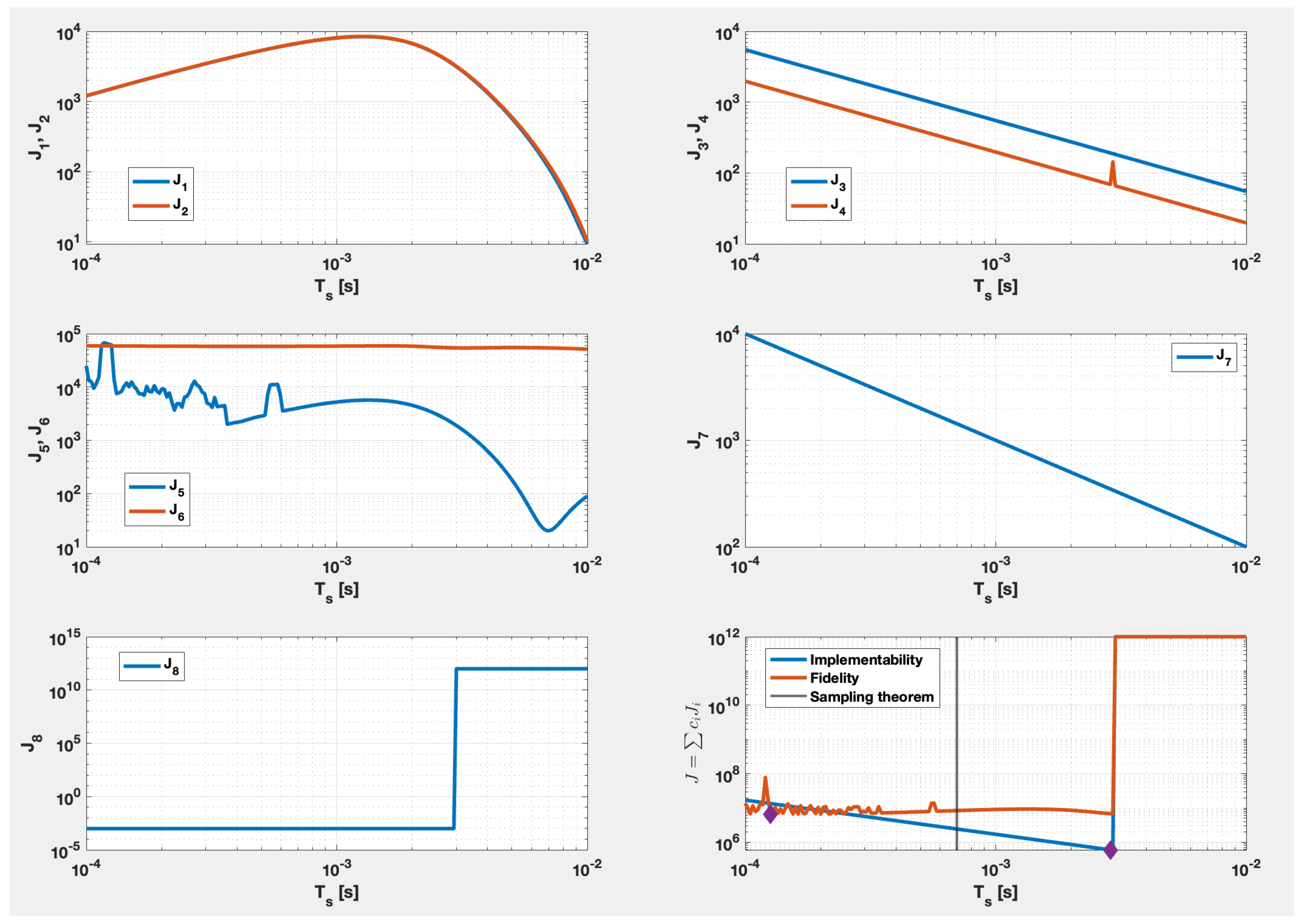
By imposing the functionals , and from Equation (23), two weighting sets – were considered as in Table 7, corresponding to two distinct experiments, the first numerical column designating emphasis on the difficulty of implementation functionals, while the second numerical column coefficients focus mainly on open-loop and closed-loop fidelity. With said coefficients, using a general-purpose PSO implementation as specified in Remark 3 [28], the optimal implementability sampling period becomes [s], while the fidelity sampling period is obtained at . To further extend the analysis, two extra sampling periods will be added in the discussion, the first representing the value obtained by applying the classical Shannon–Nyquist theorem (9), leading to a sampling period smaller than half the least time constant of the regulator, i.e., [s], while the latter relevant value is considered to be , which represents a disturbance increase on the ideal implementability sampling rate, which causes instability in the closed-loop system. Figure 7 gathers all functionals and their weighted sums in its six subfigures, while also marking the positions of , and . The open and closed-loop similarity functionals , , , are non-monotonic with respect to a variable , while the implementability functionals , , are principally monotonically decreasing. The existing exceptions appear due to numerical errors.
There are multiple approaches for implementing the two PID regulators. Both and can be fully encompassed into a biquadratic filter topology and, furthermore, a first-order structure for . The two main ones, given the simplicity of their structure, would be to implement it in parallel versus in series. For the inner regulator, the parallel topology, denoted with the superscript p can be split into three subsystems:
while the series topology, denoted with the superscript s, is:
where the equivalent normalized coefficients are obtained:
In the same manner, the parallel form of the feedforward regulator is adapted as:
with a first-order series form of:
and equivalent normalized coefficients:
3.3. Execution Time Analysis
After the discretization procedure as specified by (48) and (49), using the right-hand side notation for the coefficients in (56) and (60), the numerical values of the coefficients become as in Table 8, using the for deduced sampling rates from Section 3.2, , , , . As observed, the gain coefficient for and for , respectively, remains invariant in this set of experiments, while the remaining non-unitary coefficients vary with respect to and necessitate increasingly more decimals as the sampling rate tends to zero.
To account for the necessary word length analysis, two frequently used configurations have been considered: the first case is to store the operands, i.e., coefficients and inputs, states, outputs into 16-bit registers, considered the standard length for the RISC machine hosting the 2DOF controller, followed by a set of 32-bit length registers, which will increase the working precision, but with added execution time overhead, as modeled in continuation. Given the dynamic range of the final filter gains g, this final multiplication will be considered separately. Thus, the set for this case study will encompass the properties:
- it has a clock tick period of [s], obtainable on standard microcontrollers by configurating the phase-locked loop circuit to a lower-power setting;
- implements the second-order sections using the Direct Form II for and a series connection for the first-order term , denoted ;
- two configurations for the word lengths of the operands: 16-bit and 32-bit;
- applies saturation on output command signals ;
- applies anti-windup on the integrator term of using the back-calculation method:with the additional parameters , , represented using a 16-bit word length;
- the output measurement is gathered as a sum of impulses, with a maximum expected frequency of 80,000 impulses per 100 [ms] time unit, and each such impulse triggers a hardware interrupt with a 15 assembly operation stack commutation cost; the scaling is then performed using a multiplication with a 16-bit variable;
- accepts the reference signal as input, while accepts the error .
The mathematical operations , along with their assembly instruction correspondents as in (29) are detailed in Table 9, with an emphasis on each type of operation based on its physical significance, as written in the last column. The hyperparameters in the case of standard 16-bit word lengths have been considered with the value 1, denoting that each base arithmetical operations costs only , while the values are scaled upwards for the case when the operands exceed the word length to 32 bits. The impulse counter assembly operation cost for has been computed as 80,000 . Additionally, Table 10 totalizes the number of assembly operations based on the previous table’s description, along with computing the worst-case execution times for the three stable sampling rate values: –. As seen from the table, the optimal sampling rate solution featuring implementability emphasis occupies the microprocessor for less than of its capability in either 16 or 32-bit quantizations alike, with the Shannon theorem approach following with sufficient headroom in the scheduler algorithm, while the fidelity-based approach in this case occupies the scheduler with small margins in the case of 16-bit quantizations, and exceeds the allowed time frame in the case of the 32-bit configuration.
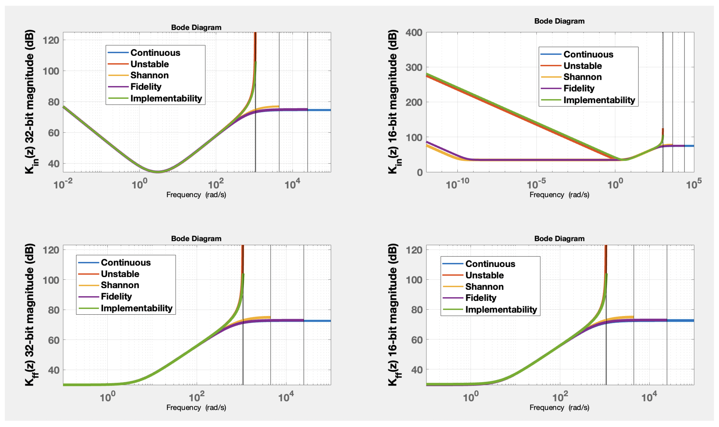
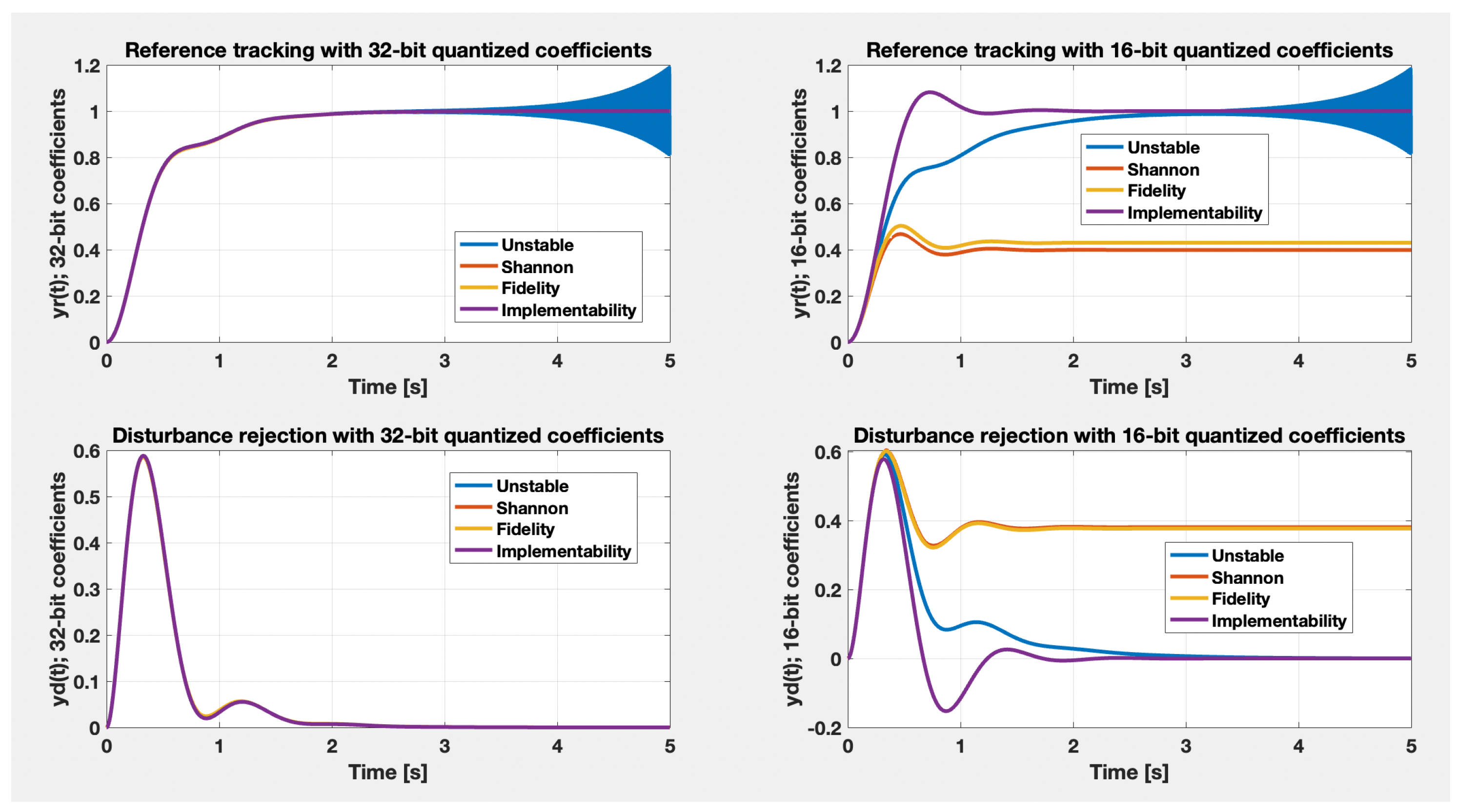
Based exclusively on the previous WCET analysis, there are several feasible solutions. In order to decide between the three sampling rate and quantization pair configurations, further analysis is performed on the frequency response of the and controllers, along with the closed-loop responses using said controllers. As such, Figure 8 and Figure 9, respectively, gather the previously said behaviors. In addition to the three sampling rates, for completeness, the fourth, unstable sampling rate is shared, along with the ideal continuous-time equivalent controllers in the frequency-response plot. In both figures, columns one and two expose the 32-bit and 16-bit quantization configurations, respectively, while the lines distinguish between the , controllers in the frequency-response figure and reference step response compared to the step disturbance responses in the time-domain simulation, respectively. The main conclusion drawn from this final pair of Figures is that the considered 2DOF control scheme is sensitive to the coefficient quantization levels, such that for and , the only acceptable solution would be to use the precise 32-bit configuration, with the exception of the implementability solution which manages to follow the imposed closed-loop transient response specifications with a reasonable degradation of the performances. The 16-bit quantization frequency responses for drastically alter the integrator effect, which, in effect, disturbs the ability of the closed-loop motor system to track reference signals and to reject step-like load torque disturbances.
To conclude the case study, the acceptable solutions are to consider the implementability-based sampling rate optimum , with practically ideal behavior if a 32-bit word length setup is acceptable, and with a small performance degradation if only the 16-bit standard word length is supported, depending also on other execution threads running in the microprocessor, not covered in this experiment.
Further extensions, as in using more complex controllers for both the tracking regulator and the feedforward component, considering cases such as fractional-order controllers or 2DOF robust control synthesis results can be treated in an analogous manner by splitting such control laws into their component second-order sections and applying the theory from Table 3 and Table 4, along with Algorithms 1 and 2, respectively.
4. Conclusions
This paper gathered a set of analysis and design tools to determine the sampling rate of one and 2DOF control structures using an optimization-based approach, along with an approach of deducing a WCET for linear and time-invariant-based regulators through a formal language model which can be implemented in an RCP software tool. The execution time model is based on a deterministic, RISC architecture, where each operation is quantified with the same base clock tick duration. The end-to-end DC motor case study emphasizes the design of the controllers for the widely used benchmark system, by also focusing on the proposed framework.
Future work will concern on an online sampling rate optimization, as it is necessary in linear-parameter varying and linear-time variant models, along with the study and analysis of the continuity property of the regulator coefficient quantization effects as a function of the sampling rate. The problem of process controllability loss is also known in the literature and will be investigated for variable sampling rates in subsequent research. The mathematical framework proposed and extended in this paper will be included in the software toolbox initially proposed by the authors in [22], with the great advantage of obtaining an end-to-end solution for RCP, starting from the continuous-time controller design up to the optimal numerical implementation of said controller on a microprocessor-based system with a given set of specifications. A separate theoretical direction would be to investigate the link between sampling rate and quantization step to guarantee that the minimum imposed performances are also fulfilled in the discrete domain.
Author Contributions
Conceptualization, M.Ş. and V.M.; methodology, M.Ş.; software, M.Ş. and V.M.; validation, M.Ş., V.M. and D.M.; formal analysis, P.D.; investigation, M.Ş.; resources, M.Ş. and V.M.; data curation, D.M.; writing—original draft preparation, M.Ş. and V.M.; writing—review and editing, V.M., D.M. and P.D.; visualization, M.Ş.; supervision, P.D.; project administration, P.D.; funding acquisition, P.D. All authors have read and agreed to the published version of the manuscript.
Funding
This paper was financially supported by the Project “Entrepreneurial competences and excellence research in doctoral and postdoctoral programs—ANTREDOC”, project co-funded by the European Social Fund financing agreement no. 56437/24.07.2019.
Institutional Review Board Statement
Not applicable.
Informed Consent Statement
Not applicable.
Data Availability Statement
Not applicable.
Conflicts of Interest
The authors declare no conflict of interest.
Abbreviations
The following abbreviations are used in this manuscript:
| 2DOF | Two-Degrees-of-Freedom |
| ADC | Analog-to-Digital Converter |
| DAC | Digital-to-Analog Converter |
| DC | Direct Current |
| DMA | Direct Memory Access |
| ISR | Interrupt Service Routine |
| LMI | Linear Matrix Inequality |
| LTI | Linear and Time-Invariant |
| MAC | Multiply-Accumulate |
| MiL | Model-in-the-Loop |
| MIMO | Multi-Input Multi-Output |
| NP | Non-deterministic Polynomial-time |
| PID | Proportional–Integral–Derivative |
| PIDF | Proportional–Integral–Derivative with Lowpass Filter |
| RAM | Random-Access Machine |
| RCP | Rapid Control Prototyping |
| SiL | Software-in-the-Loop |
| SOS | Second-Order Section |
| SIMD | Single Instruction/Multiple Data |
| SIMP | Single Instruction Stream/Multiple Instruction Pipelining |
| SISO | Single-Input Single-Output |
| WCET | Worst-Case Execution Time |
References
- Tan, L.; Jiang, J. Digital Signal Processing: Fundamentals and Applications, 3rd ed.; Elsevier: Amsterdam, The Netherlands, 2019. [Google Scholar]
- Dohnal, F.; Rerucha, V. Practical Aspects of Digital Control Systems Design—Sampling Period Choice. In Proceedings of the IFAC Programmable Devices and Systems, Ostrava, Czech Republic, 8–9 February 2000. [Google Scholar]
- Tomov, L.; Garipov, E. Choice of Sample Time in Digital PID Controllers. RECENT 2007, 8, 2. [Google Scholar]
- Bensic, T.; Varga, T.; Barukcic, M.; Stil, V.J. Optimization Procedure for Computing Sampling Time for Induction Machine Parameter Estimation. Appl. Sci. 2020, 10, 3222. [Google Scholar] [CrossRef]
- Mishra, I.; Tripathi, R.N.; Hanamoto, T. Synchronization and Sampling Time Analysis of Feedback Loop for FPGA-Based PMSM Drive System. Electronics 2020, 9, 1906. [Google Scholar] [CrossRef]
- Trusca, M.; Petreus, D.; Munteanu, R.A.; Sita, I.V.; Dobra, P. Wireless low cost embedded solution for electrical motors control. In Proceedings of the 5th European DSP Education and Research Conference (EDERC), Amsterdam, The Netherlands, 13–14 September 2012; pp. 144–148. [Google Scholar] [CrossRef]
- Duma, R.; Dobra, P.; Dobra, M.; Sita, I.V. Low cost embedded solution for BLDC motor control. In Proceedings of the 15th International Conference on System Theory, Control and Computing, Sinaia, Romania, 14–16 October 2011; pp. 1–6. [Google Scholar]
- Janus, T.; Ulanicki, B. Effects of Sampling on Stability and Performance of Electronically Controlled Pressure-Reducing Valves. J. Water Resour. Plan. Manag. 2021, 147. [Google Scholar] [CrossRef]
- Wilhelm, R.; Engblom, J.; Ermedahl, A.; Holsti, N.; Thesing, S.; Whalley, D.; Bernat, G.; Ferdin, C.; Heckmann, R.; Mitra, T.; et al. The Worst-Case Execution Time Problem—Overview of Methods and Survey of Tools. ACM Trans. Embed. Comput. Syst. 2008, 7, 1–47. [Google Scholar] [CrossRef]
- Șușcă, M.; Mihaly, V.; Morar, D.; Dobra, P. Worst-Case Execution Time Estimation for Numerical Controllers. In Proceedings of the 2022 IEEE International Conference on Automation, Quality and Testing, Robotics (AQTR), Cluj-Napoca, Romania, 19–21 May 2022; pp. 1–6. [Google Scholar] [CrossRef]
- Nghiem, T.X.; Pappas, G.J.; Alur, R.; Girard, A. Time-triggered Implementations of Dynamic Controllers. ACM Trans. Embed. Comput. Syst. (TECS) 2012, 11, 58. [Google Scholar] [CrossRef]
- Åström, K.J.; Hägglund, T. Advanced PID Control; ISA-The Instrumentation, Systems, and Automation Society: Raleigh, NC, USA, 2006. [Google Scholar]
- Skogestad, S.; Postlethwaite, I. Multivariable Feedback Control: Analysis and Design; John Wiley & Sons: Hoboken, NJ, USA, 2005. [Google Scholar]
- Mihaly, V.; Şuşcă, M.; Dulf, E.H. μ-Synthesis FO-PID for Twin Rotor Aerodynamic System. Mathematics 2021, 9, 2504. [Google Scholar] [CrossRef]
- Mihaly, V.; Şuşcă, M.; Morar, D.; Stănese, M.; Dobra, P. μ-Synthesis for Fractional-Order Robust Controllers. Mathematics 2021, 9, 911. [Google Scholar] [CrossRef]
- Gahinet, P.; Apkarian, P. Automated Tuning of Gain-Scheduled Control Systems. In Proceedings of the IEEE Conference of Decision and Control, Firenze, Italy, 10–13 December 2013. [Google Scholar]
- Mihaly, V.; Şuşcă, M.; Dobra, P. Krasovskii Passivity and μ-Synthesis Control Design for Quasi-Linear Affine Systems. Energies 2021, 14, 5571. [Google Scholar] [CrossRef]
- Taguchi, H.; Araki, M. Two-degree-of-freedom PID Controllers—Their Functions and Optimal Tuning. In Proceedings of the IFAC Digital Control: Past. Present and Future of PID Control, Terrassa, Spain, 5–7 April 2000. [Google Scholar]
- Wang, D.; Liu, T.; Sun, X.; Zhong, C. Discrete-time domain two-degree-of-freedom control design for integrating and unstable processes with time delay. ISA Trans. 2016, 63, 121–132. [Google Scholar] [CrossRef] [PubMed]
- Oviedo, J.J.E.; Boelen, T.; van Overschee, P. Robust advanced PID control (RaPID): PID tuning based on engineering specifications. IEEE Control Syst. Mag. 2006, 26, 15–19. [Google Scholar] [CrossRef]
- Șușcă, M.; Mihaly, V.; Morar, D.; Dobra, P. Quasi-Optimal Sampling Time Computation for LTI Controllers. In Proceedings of the 6th IFAC Conference on Intelligent Control and Automation Sciences, ICONS, Cluj-Napoca, Romania, 13–15 July 2022; Volume 55, pp. 87–92. [Google Scholar] [CrossRef]
- Şuşcă, M.; Mihaly, V.; Stănese, M.; Morar, D.; Dobra, P. Unified CACSD Toolbox for Hybrid Simulation and Robust Controller Synthesis with Applications in DC-to-DC Power Converter Control. Mathematics 2021, 9, 731. [Google Scholar] [CrossRef]
- Cormen, T.H.; Leiserson, C.E.; Rivest, R.L.; Stein, C. Introduction to Algorithms, 3rd ed.; MIT Press: Cambridge, MA, USA, 2009. [Google Scholar]
- Șușcă, M.; Mihaly, V.; Dobra, P. Fixed-Point Uniform Quantization Analysis for Numerical Controllers. In Proceedings of the 2022 IEEE Conference on Decision and Control (CDC), Cancún, Mexico, 6–9 December 2022. [Google Scholar]
- Whorton, M.; Yang, L.; Hall, R. Similarity Metrics for Closed Loop Dynamic Systems. In Proceedings of the AIAA Guidance, Navigation and Control Conference and Exhibit, Honolulu, HI, USA, 18–21 August 2008. [Google Scholar] [CrossRef]
- Hsieh, G.C.; Safonov, M.G. Conservatism of the gap metric. IEEE Trans. Autom. Control 1993, 38, 594–598. [Google Scholar] [CrossRef]
- Vinnicombe, G. Frequency domain uncertainty and the graph topology. IEEE Trans. Autom. Control 1993, 38, 1371–1383. [Google Scholar] [CrossRef]
- Kennedy, J.; Eberhart, R. Particle Swarm Optimization. In Proceedings of the IEEE International Conference on Neural Networks, Perth, WA, Australia, 27 November–1 December 1995; Volume 4, pp. 1942–1948. [Google Scholar]
- da Silva, L.R.; Flesch, R.C.C.; Normey-Rico, J.E. Analysis of Anti-windup Techniques in PID Control of Processes with Measurement Noise. In Proceedings of the 3rd IFAC Conference on Advances in Proportional-Integral-Derivative Control PID, Ghent, Belgium, 9–11 May 2018; Volume 51, pp. 948–953. [Google Scholar] [CrossRef]
- Tarbouriech, S.; Turner, M. Anti-windup design: An overview of some recent advances and open problems. IET Control Theory Appl. 2009, 3, 1–19. [Google Scholar] [CrossRef]
- Singh, R.P.; Vashishtha, A.K.; Krishna, R. 32 Bit re-configurable RISC processor design and implementation for BETA ISA with inbuilt matrix multiplier. In Proceedings of the Sixth International Symposium on Embedded Computing and System Design (ISED), Patna, India, 15–17 December 2016; pp. 112–116. [Google Scholar] [CrossRef]
- Salim, A.J.; Samsudin, N.R.; Salim, S.I.M.; Soo, Y. Multiply-accumulate instruction set extension in a soft-core RISC Processor. In Proceedings of the 10th IEEE International Conference on Semiconductor Electronics (ICSE), Kuala Lumpur, Malaysia, 19–21 September 2012; pp. 512–516. [Google Scholar] [CrossRef]
- Murakami, K.; Irie, N.; Kuga, M.; Tomita, S. SIMP (single Instruction Stream/multiple Instruction Pipelining): A Novel High-speed Single-processor Architecture. In Proceedings of the 16th Annual International Symposium on Computer Architecture, Jerusalem, Israel, 28 May–1 June 1989; pp. 78–83. [Google Scholar] [CrossRef]
- Proakis, J.G.; Manolakis, D.G. Digital Signal Processing: Principles, Algorithms and Applications, 5th ed.; Pearson, Prentice Hall: Upper Saddle River, NJ, USA, 2022; ISBN 9780137348657. [Google Scholar]
- Essl, G. Topological IIR Filters Over Simplicial Topologies via Sheaves. IEEE Signal Process. Lett. 2020, 27, 1215–1219. [Google Scholar] [CrossRef]
- Marjanovic, J. Deutsches Elektronen-Synchrotron (DESY), Low vs. High Level Programming for FPGA. In Proceedings of the 7th International Beam Instrumentation Conference, IBIC2018, Shanghai, China, 9–13 September 2018; JACoW Publishing: Geneva, Switzerland, 2018. ISBN 978-3-95450-201-1. [Google Scholar] [CrossRef]
Figure 1.
Numeric regulator with a specified sampling rate and its corresponding interface consisting of a sample and hold with the analog-to-digital converter, along with the digital-to-analog converter followed by a sample and hold circuit.
Figure 1.
Numeric regulator with a specified sampling rate and its corresponding interface consisting of a sample and hold with the analog-to-digital converter, along with the digital-to-analog converter followed by a sample and hold circuit.

Figure 2.
Two-degrees-of-freedom (2DOF) numerical control structure with components and , designed for the process models with disturbance dynamics .
Figure 2.
Two-degrees-of-freedom (2DOF) numerical control structure with components and , designed for the process models with disturbance dynamics .

Figure 3.
Rapid control prototyping relationship between the formal sets and functionals necessary to perform a worst-case execution time analysis for a regulator in the production context .
Figure 3.
Rapid control prototyping relationship between the formal sets and functionals necessary to perform a worst-case execution time analysis for a regulator in the production context .

Figure 4.
Sequence diagram illustrating the regulator interrupt service routine execution among higher and lower priority threads for the duration of one sampling period [10].
Figure 4.
Sequence diagram illustrating the regulator interrupt service routine execution among higher and lower priority threads for the duration of one sampling period [10].

Figure 5.
Closed-loop two-degree-of-freedom (2DOF) position control structure for the DC motor system with a control voltage input and a disturbance load torque . The 2DOF structure has an inner-loop component designed for disturbance rejection and a feedforward component for good servo compensation.

Figure 6.
Closed-loop continuous-time domain simulations; step reference responses along with step disturbance rejections considering 1DOF regulators designed for servo tracking, disturbance rejection, and for performance in both cases, respectively.
Figure 6.
Closed-loop continuous-time domain simulations; step reference responses along with step disturbance rejections considering 1DOF regulators designed for servo tracking, disturbance rejection, and for performance in both cases, respectively.

Figure 7.
Functionals , corresponding to , respectively, and their weighted sum as in Equation (23) for both performed experiments. Besides the implementability and fidelity cases, a classical sampling-theorem approach is illustrated.
Figure 7.
Functionals , corresponding to , respectively, and their weighted sum as in Equation (23) for both performed experiments. Besides the implementability and fidelity cases, a classical sampling-theorem approach is illustrated.

Figure 8.
DC motor example regulator frequency magnitude responses; the first line gathers the inner regulator with 32-bit and 16-bit quantized regulator coefficients, respectively, while the second line gathers the feedforward controller in the same 32-bit and 16-bit configurations. For completeness, the continuous-time ideal regulators and were also added alongside their discrete-time counterparts.

Figure 9.
DC motor example closed-loop step responses using the proposed 2DOF control structure; the first line gathers the reference tracking behavior with 32-bit and 16-bit quantized regulator coefficients, respectively, while the second line gathers the disturbance rejection behavior in the same 32-bit and 16-bit configurations.


Table 1.
Formal operators necessary for the implementation of LTI-based control laws.
| # | Operator | Domain | Definition | Observations |
|---|---|---|---|---|
| 1 | Addition | bilinear | ||
| 2 | Multiplication | homogenous | ||
| 3 | Saturation | nonlinear | ||
| 4 | Anti-windup | various [12,29,30] | for integrators | |
| 5 | Load/Store | bilinear | ||
| 6 | Null | for delays |
Table 2.
Base assembly operations for a Random-Access Machine model used in an LTI-based control system context.
Table 2.
Base assembly operations for a Random-Access Machine model used in an LTI-based control system context.
| # | Operator | Abbreviation | Part of Operation | Observations |
|---|---|---|---|---|
| 1 | No operation | NOP | – | |
| 2 | Memory fetch | MF | SIMP | |
| 3 | Memory store | MS | SIMP | |
| 4 | Add | ADD | SIMP, MAC, SIMD | |
| 5 | Multiply | MUL | SIMP, MAC, SIMD | |
| 6 | Binary shift | SH | SIMP, SIMD | |
| 7 | Jump | JMP | – | |
| 8 | Compare | CMP | SIMP |
Table 3.
Digital biquadratic topology implementations; all difference equations implement the same input-output second-order transfer function, but differ through the configurations of the state signals.
Table 3.
Digital biquadratic topology implementations; all difference equations implement the same input-output second-order transfer function, but differ through the configurations of the state signals.
| IIR SOS Topology | Difference Equation | |
|---|---|---|
| Direct Form I (DFI) | , , | |
| Direct Form II (DFII) | , , | |
| , , | ||
| , , |
Table 4.
Digital FIR filter topology implementations; all difference equations implement the same input-output Nth order transfer function, but vary through the configuration of the accumulator.
Table 4.
Digital FIR filter topology implementations; all difference equations implement the same input-output Nth order transfer function, but vary through the configuration of the accumulator.
| FIR Topology | Difference Equation | |
|---|---|---|
| Direct Form | , , | |
| Direct Form Transposed | , , | |
| Symmetric | ||
| Anti-symmetric |
Table 5.
DC motor physical parameters.
| Parameter | Value | Parameter | Value |
|---|---|---|---|
| R | L | [H] | |
| [Nm·A/V2] | [Nm] | ||
| J | [kg · m2/s2] | [V·s/rad] |
Table 6.
Regulator designs leading to the proposed 2DOF control and their corresponding coefficients.
Table 6.
Regulator designs leading to the proposed 2DOF control and their corresponding coefficients.
| Regulator | b | c | ||||
|---|---|---|---|---|---|---|
| PID (1DOF): tracking | 21.0666 | 8.757 | 7.7497 | 0.0014717 | 1 | 1 |
| PID (1DOF): disturbance rejection | 52.6665 | 70.0560 | 7.7497 | 0.0014717 | 1 | 1 |
| PID (2DOF) | 52.6665 | 70.0560 | 7.7497 | 0.0014717 | 0.4 | 0.2 |
Table 7.
Functional weighting coefficients for the two considered experiments of the DC motor case study: main focus on implementability of the resulting controller versus the focus on fidelity compared to the continuous-time control counterpart.
Table 7.
Functional weighting coefficients for the two considered experiments of the DC motor case study: main focus on implementability of the resulting controller versus the focus on fidelity compared to the continuous-time control counterpart.
| Parameter | Implementability Case Value | Fidelity Case Value |
|---|---|---|
| 0.1 | 100 | |
| 0.1 | 100 | |
| 2000 | 1 | |
| 2000 | 1 | |
| 0.1 | 300 | |
| 0.1 | 100 | |
| 200 | 1 | |
| [s] | [s] |
Table 8.
DC motor case study discrete-time ideal coefficients using the deduced sampling rates.
| Coefficient | ||||
|---|---|---|---|---|
| g: | ||||
| : | 1 | 1 | 1 | 1 |
| : | ||||
| : | ||||
| : | ||||
| : | ||||
| g: | ||||
| : | 1 | 1 | 1 | 1 |
| : | ||||
| : |
Table 9.
Encountered operations in the implementation of the 2DOF structure for the DC motor case study in the hypothesis of a base word length of bits and two considered quantization levels for the controller coefficients: 16-bit and 32-bit lengths, respectively.
Table 9.
Encountered operations in the implementation of the 2DOF structure for the DC motor case study in the hypothesis of a base word length of bits and two considered quantization levels for the controller coefficients: 16-bit and 32-bit lengths, respectively.
| Observations for | ||||||||
|---|---|---|---|---|---|---|---|---|
| 1 | 14 | 18 | 8 | 13 | 1 | 2 | ||
| 1 | 4 | 5 | 2 | 3 | 1 | 2 | ||
| 1 | 6 | 5 | 4 | 4 | 1 | 6 | ||
| 8 | 1 | 1 | 1 | 1 | 1 | 2 | ||
| 20 | 1 | 1 | 0 | 0 | 1 | 6 | Integrator anti-windup | |
| 1 | 1 | 0 | 0 | 1 | 1 | impulse counter | ||
| 1 | 1 | 1 | 0 | 0 | 1 | 6 | scaling | |
| 1 | 1 | 1 | 0 | 0 | 1 | 2 | ||
| 1 | 3 | 3 | 0 | 0 | 1 | 2 | ||
| 1 | 2 | 2 | 1 | 1 | 1 | 2 | ||
| 1 | 2 | 2 | 1 | 1 | 1 | 2 |
Table 10.
DC motor case study WCET analysis in the conditions from Table 9, by emphasizing the number of assembly operations necessary to implement the 2DOF structure comprised of and , along with the processor usage level for the three stable sampling rate values.
Table 10.
DC motor case study WCET analysis in the conditions from Table 9, by emphasizing the number of assembly operations necessary to implement the 2DOF structure comprised of and , along with the processor usage level for the three stable sampling rate values.
| 77 | 24 | 81 | 30 | 246 | 64 | 250 | 76 | |
| 101 | 111 | 310 | 326 | |||||
| WCET[s] | 429[s] | 439[s] | 638[s] | 654[s] | ||||
| WCET[s] | 101[s] | 111[s] | 310[s] | 326[s] | ||||
| WCET[s] | 170[s] | 180[s] | 379[s] | 395[s] | ||||
Publisher’s Note: MDPI stays neutral with regard to jurisdictional claims in published maps and institutional affiliations. |
© 2022 by the authors. Licensee MDPI, Basel, Switzerland. This article is an open access article distributed under the terms and conditions of the Creative Commons Attribution (CC BY) license (https://creativecommons.org/licenses/by/4.0/).
Share and Cite
MDPI and ACS Style
Şuşcă, M.; Mihaly, V.; Morar, D.; Dobra, P. Sampling Rate Optimization and Execution Time Analysis for Two-Degrees-of-Freedom Control Systems. Mathematics 2022, 10, 3449. https://0-doi-org.brum.beds.ac.uk/10.3390/math10193449
AMA Style
Şuşcă M, Mihaly V, Morar D, Dobra P. Sampling Rate Optimization and Execution Time Analysis for Two-Degrees-of-Freedom Control Systems. Mathematics. 2022; 10(19):3449. https://0-doi-org.brum.beds.ac.uk/10.3390/math10193449
Chicago/Turabian StyleŞuşcă, Mircea, Vlad Mihaly, Dora Morar, and Petru Dobra. 2022. "Sampling Rate Optimization and Execution Time Analysis for Two-Degrees-of-Freedom Control Systems" Mathematics 10, no. 19: 3449. https://0-doi-org.brum.beds.ac.uk/10.3390/math10193449
Note that from the first issue of 2016, this journal uses article numbers instead of page numbers. See further details here.