

The Relation Dimension in the Identification and Classification of Lexically Restricted Word Co-Occurrences in Text Corpora

1
NLP Group, Pompeu Fabra University, 08018 Barcelona, Spain
2
Catalan Institute for Research and Advanced Studies (ICREA) and NLP Group, Pompeu Fabra University, 08018 Barcelona, Spain
*
Author to whom correspondence should be addressed.
Mathematics 2022, 10(20), 3831; https://0-doi-org.brum.beds.ac.uk/10.3390/math10203831
Submission received: 1 September 2022
/
Revised: 2 October 2022
/
Accepted: 4 October 2022
/
Published: 17 October 2022
(This article belongs to the Special Issue Advances in Machine Learning Methods for Natural Language Processing and Computational Linguistics)
Abstract
:The speech of native speakers is full of idiosyncrasies. Especially prominent are lexically restricted binary word co-occurrences of the type high esteem, strong tea, run [an] experiment, war break(s) out, etc. In lexicography, such co-occurrences are referred to as collocations. Due to their semi-decompositional nature, collocations are of high relevance to a large number of natural language processing applications as well as to second language learning. A substantial body of work exists on the automatic recognition of collocations in textual material and, increasingly also on their semantic classification, even if not yet in the mainstream research. Especially classification with respect to the lexical function (LF) taxonomy, which is the most detailed semantically oriented taxonomy of collocations available to date, proved to be of real use to human speakers and machines alike. The most recent approaches in the field are based on multilingual neural graph transformer models that use explicit syntactic dependencies. Our goal is to explore whether the extension of such a model by a semantic relation extraction network improves its classification performance or whether it already learns the corresponding semantic relations from the dependencies and the sentential contexts, such that an additional relation extraction network will not improve the overall performance. The experiments show that the semantic relation extraction layer indeed improves the overall performance of a graph transformer. However, this improvement is not very significant, such that we can conclude that graph transformers already learn to a certain extent the semantics of the dependencies between the collocation elements.
1. Introduction
The language of native speakers often contains wordings with varying degrees of semantic decomposition. The most overt are idioms, such as, e.g., it is a piece of cake meaning ‘easy’ or to be under the weather meaning ‘to feel ill’, but even more frequent and relevant to language proficiency of a speaker or machine are lexically restricted binary word co-occurrences, in which one of the two syntactically bound lexical items restricts the selection of the other item. Consider a statement in an CNN sports commentary from 9 July 2022:
Having taken an early lead, Rybakina almost gave up her advantage soon after, needing to fend off multiple break points before eventually taking a two-game lead in the set.
Already, this short statement contains three of such co-occurrences: take [a] lead, give up advantage, and fend off [a] break point, with lead, advantage, and break point restricting the selection of take, give up, and fend off respectively. While for an English native speaker, these co-occurrences may appear to involve no idiosyncrasy, one can clearly recognize it from the multilingual angle. Thus, in German, instead of the literal nehmen, one would use gehen ‘go’ to translate take in take [a] lead: in Führung gehen, lit. ‘to go into lead’. In Spanish, give up in co-occurrence with ventaja ‘advantage’ will be translated as ceder ‘cede’: ceder [una] ventaja, and in French fend off will be translated in the context of breakpoint as repousser ‘repell’: repousser [un] point de rupture. In contrast, in the context of walk, take would be translated into German as machen ‘make’: einen Spaziergang machen, lit. ‘make a walk’, in the context of rights, give up would be translated into Spanish as renunciar ‘renounce’: renunciar a sus derechos, lit.‘renounce to one’s rights’, and in the context of competition, fend off would be translated into French as contrer: contrer la concurrence. Note that at the same time lead, advantage, break point, walk, rights, and competition will always be translated literally.
Lexically resticted word co-occurrences are of extremely high relevance to second language learners [1,2,3,4,5,6] and many Natural Language Processing (NLP) applications, including, e.g., natural language generation [7,8], machine translation [9], semantic role labeling [10] and word sense disambiguation [11]. Thus, language learners must memorize them by heart and master even fine-grained semantic differences between them (as Mel’čuk and Wanner [12] show, while a certain semantic feature-based analogy (or, in other words, generalization) in the formation of such co-occurrences is possible, even for co-occurrences with emotion nouns, which are considered to be very homogeneous, major divergences prevail). For instance, a language learner should know the difference between lodge [a] complaint and voice [a] complaint or between receive [a] compensation and have [a] compensation. Automatic text generation appears more natural if it uses idiosyncratic word co-occurrences (compare, e.g., John walks every morning on the beach vs. John takes a walk on the beach every morning); semantic role labeling needs to capture in take a walk that John is not the recipient of the walk, but rather the actor, and machine translation from English to German needs to translate take in co-occurrence with walk as machen ‘make’ and not as nehmen ‘take’. Language models as commonly used in modern NLP partially capture such co-occurrences, but it has been shown that even if downstream applications use state-of-the-art language models, they benefit from additional information on restricted lexical co-occurrence; see, e.g., the experiments of Maru et al. on Word Sense Disambiguation [11], in which they use explicit lists of semantically labeled lexical co-occurrences. Therefore, it is surprising that so far, the automatic acquisition and semantic labeling of lexically resticted co-occurrences has not been given close attention in mainstream research on distributional semantics. Most of the work focused on a mere identification of statistically significant lexical co-occurrences in text corpora; see, among others, [7,13,14,15]. This is insufficient. Firstly, not all statistically significant word co-occurrences are, in fact, lexically restricted, and, secondly, as illustrated above, in order to be of real use, their semantics must be also known.
In a series of experiments, Wanner et al. (see, for instance, [16,17,18,19]) work with precompiled lists of co-occurrences, which they classify with respect to the fine-grained semantic typology of lexical functions (LFs) [20]. In another work [21], they go one step further by identifying instances from precompiled co-occurrence lists in text corpora and using then their sentential contexts as additional information for classification. Most recently, Espinosa-Anke et al. [22] use in their graph transformer-based model, in addition to the sentential context, the syntactic dependencies between the elements of the co-occurrences and thus take into account lexicographic studies [20] that identify syntactic dependency as one of the prominent characteristics of the individual semantic categories of the co-occurrences. However, another crucial feature of lexically restricted co-occurrences remained so far unconsidered in NLP: between its elements, not only a syntactic but also a semantic dependency holds (although Espinosa-Anke et al. explicitly point out the existence of a semantic dependency between the elements in lexically restricted word co-occurrences, they do not model it in explicit terms: the elements that form the co-occurrence are identified separately using the BIO-tagging strategy [23]).
In view of the continuous significant advances shown by semantic relation extraction techniques (http://nlpprogress.com/english/relationship_extraction.html, accessed on 15 July 2022), our goal is to explore whether the extension of a graph transformer-based model for the identification and classification of lexically restricted co-occurrences by a state-of-the-art semantic relation extraction network can contribute to an increase of the performance. Our exploration is motivated by the fact that (i) current approaches still struggle with correctly classifying some less frequent categories of lexically restricted word co-occurrences, and (ii) especially semantically similar categories are systematically confused, which is detrimental in particular for such applications as second language learning. Semantic relation techniques are a promising means to remedy this problem.
To this end, we design an LF relation–extraction model that is inspired by [24] and carry out with this model two kinds of experiments. In the first experiment, we tackle a classical classification task to assess the stand-alone performance of the adapted model and thus its suitability to form part of an extended graph transformer-based model. Given a dataset with lexically restricted co-occurrences in their sentential contexts, we classify the co-occurrences with respect to the LF typology. In the second experiment, we use the output of the identification stage of the model of Espinosa-Anke et al. [22] and feed it as input to an LF relation extraction network. Our experiments show that relation extraction indeed helps to increase the quality of lexically restricted word co-occurrence identification and classification. In particular, relation extraction ensures a better distinction between some of the categories of co-occurrences, which are notoriously confused by other state-of-the-art techniques. On the other hand, the quality increase is limited—which allows for some conclusions with respect to an implicit representation of semantic relation information by graph transformers.
The contributions of our work can thus be summarized as follows:
- We adapt a generic relation extraction framework to the problem of lexically restricted word co-occurrence classification.
- We show that neural relation extraction techniques that have not been used for the classification of lexically restricted word co-occurrences so far are a suitable means to account for the relational nature of such co-occurrences and can compete in their performance with, e.g., the most recent BIO tagging technique. This means that if the goal is to simultaneously identify and classify lexically restricted and semantic relations, relation extraction techniques can be successfully used.
- We demonstrate that the neural relation extraction techniques distinguish better between notoriously confused categories of lexically restricted word co-occurrences than the state-of-the-art techniques. This can be of high relevance to applications that focus on these categories.
- Our contrastive analysis of the BIO tagging technique, which receives as input syntactic dependency information only, and the proposed relation extraction technique suggests that the graph transformers used in the BIO tagging technique already capture the category-specific semantics of the lexically restricted word co-occurrences. This outcome contributes to the research on the types of knowledge captured by neural models.
The remainder of the article is structured as follows. The next section (Section 2) contains some background on lexically restricted co-occurrences. In Section 3, we provide an overview of the state of the art of the research on the identification and classification of such co-occurrences. Section 4 introduces the Graph-Trased transformer model (Gr2C-Tr) of Espinosa-Anke et al. [22] and its extension by a relation extraction network. Section 5 describes the experiments that have been carried out and their results, which are discussed in Section 6. Section 7, finally, draws the conclusions from our experiments and outlines some lines of relevant future work.
2. Background on Lexically Restricted Word Co-Occurrences
In lexicology and lexicography, lexically restricted word co-occurrences have been studied under the heading of collocations [25,26,27,28]. The item that restricts the selection of the other item is referred to as the base and the restricted item is the collocate. Note, however, that the original notion of collocation as introduced by J.R. Firth [29] is broader: it merely implies statistically significant word co-occurrence. In other words, any combination of words that appear together sufficiently often are considered to be collocations, among them, e.g., doctor–hospital, hospital–pandemic, or pandemic–mask. As can be observed, in these examples, no lexical restriction is imposed by one of the lexical items on the other item, i.e., there is no base and no collocate. Most of the work on automatic word co-occurrence identification is based on this notion of collocation (see Section 3 below). Obviously, this is not to say that both notions are disjoint. On the contrary, lexically restricted co-occurrences will often (although by far not always) be statistically significant; see, e.g., strong tea, contagious disease, or come [to] power.
In contrast to the mainstream research in NLP, we use the notion of collocation as introduced in lexicology/lexicography. As already mentioned above, this notion implies that between the base and the collocate of a concrete co-occurrence, a specific semantic relation, which is expressed by the collocate, and a specific syntactic dependency hold. Based on this relation and dependency, collocations can be typified. For instance, take a walk, give a lecture, make a proposal belong to the same type: take, give, and make express the same semantic relation with their respective base (namely ‘perform’ or ‘carry out’), and all of them take their respective base as a direct object. The same applies to thunderous applause, heavy storm, high temperature: here, thunderous, heavy, and high all express the relation ‘intense’.
The most fine-grained semantically-oriented typology of collocations available to date is the typology of lexical functions (LFs) [20]. An LF is defined as a function that delivers for a base B a set of synonymous collocates that express the meaning of f. LFs are assigned Latin abbreviations as labels; cf., e.g., “Oper1” (“operare” ‘perform’): Oper1(walk) = {take, do, have}; “Magn” (“magnum” ‘big’/‘intense’): Magn(applause) = {thunderous, deafening, loud, …}. But each LF can also be considered as a specific lexico-semantic relation between the base and the collocate of a collocation in question [30]. Table 1 displays the subset of the relations we experiment with along with their corresponding LF names and illustrative examples.
3. Related Work: Research on Lexically Restricted Word Co-Occurrences in NLP
With the increasingly prominent objective to understand in depth the behavior of neural language models, the research on restricted word co-occurrences is about to go beyond the core tasks of their identification and classification. Thus, there has been some recent tentative research on the use of lexical co-occurrences as probes in the context of the exploration of the representation of non-compositional meaning in neural language models [32,33]. Still, the two core tasks, i.e., (i) identification of lexical co-occurrences in text corpora, and (ii) semantic classification of available co-occurrence instances—for instance, in terms of the LF or any other available typology, continue to be active research topics. Most often, one of these two tasks is addressed. However, more recently, both tasks have also been tackled, either in sequence or together, by one model. In what follows, we review some representative works for each of these constellations.
3.1. Identification of Lexical Co-Occurrences
As already mentioned in the Introduction and in Section 2, most of the work on lexical co-occurrences focuses on the identification of statistically restricted word co-occurrences in text corpora. The most straightforward of them operate with a co-occurrence frequency of n-grams as an association measure [34,35]. The majority uses statistical measures such as, e.g., (Pointwise) Mutual Information (PMI) [13] or its variants [14,36], likelihood-ratio [37], or t-score [38]. For detailed contrastive reviews of different association measures for restricted word co-occurrence identification, see, among others, [15,39,40,41]. In some cases, the statistical measures are complemented by morphological [42,43] and/or syntactic [44,45,46] patterns that are characteristic for restricted word co-occurrences. Several authors focus on one syntactic pattern only, such as, e.g., Breidt [38], who targets verb–noun co-occurrences in German or even a specific profile of a single syntactic pattern. In this context, in particular, the identification of support (or light) verb constructions (SVCs/LVCs) has been a prominent topic of research. SVCs are captured by the Oper- (and partially by the Real-) families of LFs; cf., e.g., [32,47,48,49,50,51].
3.2. Classification of Precompiled Lists of Lexical Co-Occurrences
The lists of co-occurrences identified in text corpora or retrieved from collocation dictionaries, which use a classification schema that is either too broad or too heterogeneous for use in NLP and/or SLL (such as, e.g., the Oxford Collocations Dictionary or the MacMillan Collocations Dictionary) or different in its nature (such as, e.g., the REDES dictionary of Spanish (REDES presents restricted word co-occurrences in the entries for collocates rather than bases)), can serve as input to classification algorithms. The most common classification schema has been the LF typology or its generalization, although some other more coarse-grained schemata have also been applied; see, e.g., [21,52].
To the best of our knowledge, Wanner [16] was the first to propose the classification of lexically restricted co-occurrences, i.e., collocations in the sense used in this paper, with respect to the LF typology on a limited number of precompiled instances of the nine most common LFs in Spanish. The experiments involved runs on collocations from the field of emotions and runs on collocations from a variety of other semantic fields. The idea was that the semantics of an LF can be captured by the semantic features of the collocates and bases of a representative selection of instances of this LF, such that when these features are combined, a prototypical representation (or centroid) of this LF is obtained. The semantic profile of a new binary word co-occurrence can then be matched against the morpho-syntactic pattern of each LF and the semantic profile of its centroid. The LF with the best match is chosen as the LF to be assigned to the candidate co-occurrence. Features assigned to a lexical item in EuroWordNet [53] (i.e., the members of its synset and its base and top concepts) serve as semantic features of the profile of this item. The quality (precision, recall and F1-score) obtained during the emotion field experiments was high (the lowest F1-score was 0.78 for IncepFunc1; for ContOper1 and FinFunc0, an F1-score of 1.0 was achieved); for the cross-field runs, the figures were lower but still reasonable (the lowest F1-score was 0.58 for Real2). In [17,18], the same lists of LF instances and the same EuroWordNet-based semantic representation of LF instances have been used to test three standard Machine Learning techniques: Nearest Neighbors (NN), Naïve Bayes (NB), and Tree-Augmented Network (TAN), with a comparable resulting performance. Gelbukh and Kolesnikova [54] carried out similar experiments with a broad range of traditional ML techniques and a somewhat more restricted semantic representation in terms of the hypernyms of the verbal and noun elements of collocations.
3.3. Joint Identification and Classification of Lexical Co-Occurrences
The identification of one specific type of lexical co-occurrence, such as, e.g., the SVCs mentioned in Section 3.1, or preposition–verb constructions [55,56] can be considered, in a sense, as joint identification and classification. Examples of the simultaneous identification and semantic classification of lexical co-occurrences in terms of a more variant typology (such as the LF typology) are [22,57,58].
4. The Relation Dimension in Collocation Classification
As repeatedly pointed out above, between the lexical items of a collocation, a syntactic dependency and a semantic dependency hold. Espinosa-Anke et al. [22] exploit the syntactic dependency to identify and classify collocations in corpora using a graph transformer model that identifies and classifies the collocation elements separately in a sequence-tagging manner for English, French, and Spanish. The assessment of the performance (precision, recall, and F1-score) figures and the confusion matrices provided in [22] suggest that the performance ceiling has not been reached yet. Especially, the confusion between instances of common LFs such as Oper1, Real1, and Real2 calls for further research. One option that needs exploration is whether an explicit consideration of the semantic dependency between the base and collocate elements would contribute to an increase of the classification performance.
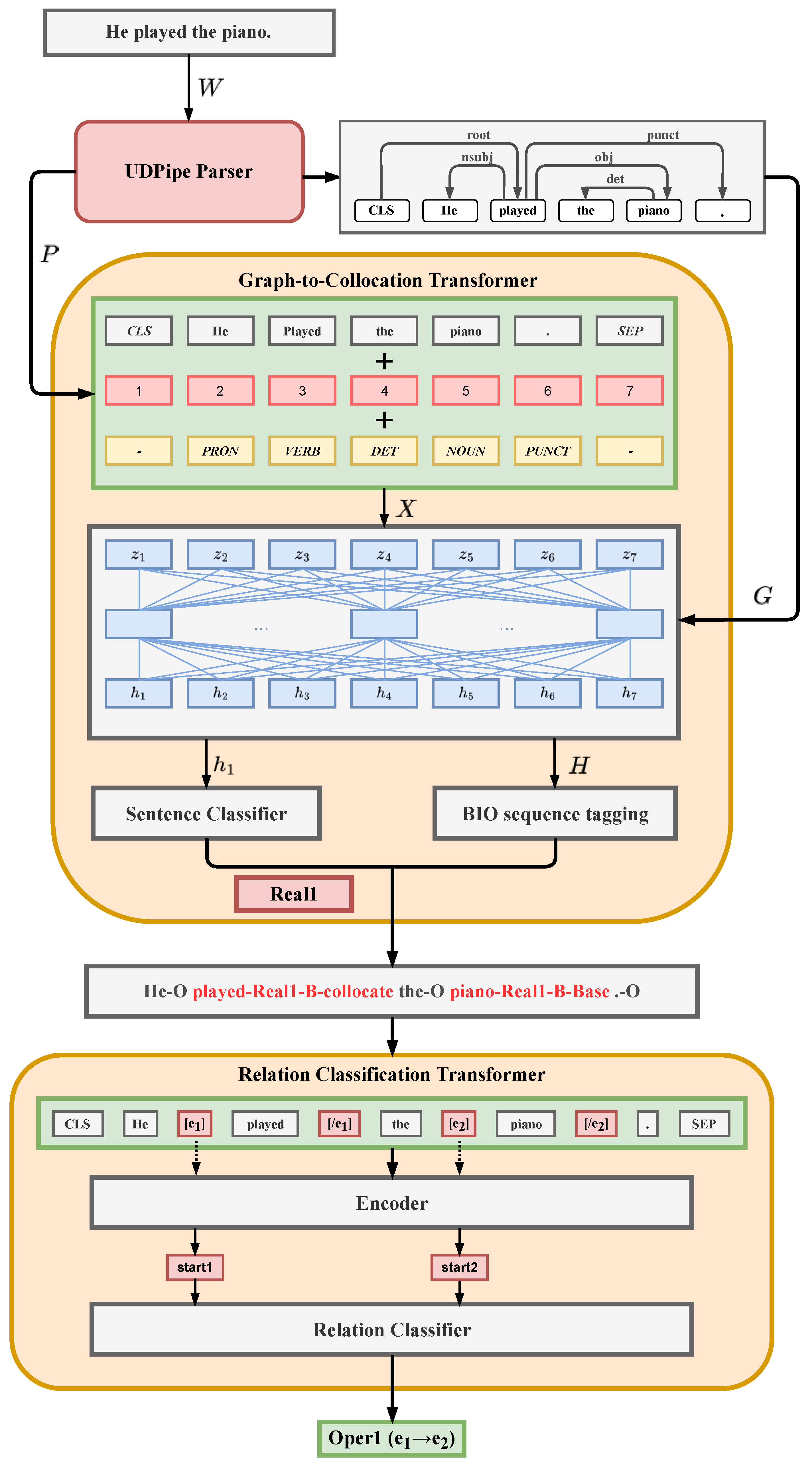
For this purpose, we adapt the relation extraction-driven model outlined in [24] for collocation classification on top of the predictions made by the model of Espinosa-Anke et al. (=base model), such that it accounts even for slight differences in meaning and is thus able to better distinguish between semantically similar LFs. Since the base model provides the position of the extracted collocation parts in the considered sequence of tokens, its outcome can be used as input for advanced relation classification models that require the explicit position of entities participating in relation as a signal for classification. Figure 1 sketches the overall architecture of our model.
In what follows, we first introduce Espinosa-Anke’s original Graph-to-Collocation Transformer (G2C-Tr) model that serves as a collocation candidate provider (the introduction mirrors the description in [22]) and then discuss the architecture of the relation extraction-driven classification model in more detail.
4.1. G2C Transformer Model
G2C-Tr is a suite of BERT-based multitask models for the joint binary classification of a sentence with respect to the occurrence of any LF-instances in it and the LF-instance BIO sequence tagging in this sentence. The task of sentence classification has been added to create a multitask setup because multitasking proved to improve the performance of the neural models for each of the tasks involved [59].
The upper part of Figure 1 illustrates the model. Given the input sentence , a pre-trained Universal Dependency (UD) parser is used to obtain the dependency graph G and Part-of-Speech (PoS) tags as input to G2C-Tr, which predicts the BIO-tagged sentence as follows:
where is the encoder of the model and is the decoder. is the contextualized vector representation, and T is the length of the tokenized sequence. The parameters of are frozen for training.
computes the contextualized vector embeddings H as the sum of pre-trained token embeddings of BERT, position embeddings, and PoS tag embeddings using a modified version of the Transformer attention mechanism to inject the syntactic dependency information. In each Transformer layer, given as the output representations of the previous layer, the attention weights are calculated as a Softmax over the attention scores , which is defined as:
where are learned query and key parameters. is the graph relation embedding matrix, learned during training, is the dimension of hidden vectors, d is the head dimension of the self-attention module, and is the overal number of dependency labels. is the one-hot vector representing both the relation and direction of syntactic relation between token and , so selects the embedding vector for the appropriate syntactic relation.
To obtain the output representations (H), Vaswani’s [60] original mechanism for the position-wise feed-forward layer and layer normalization is used.
calculates the sentence classification output as:
with i as the index of the sentence that is to be classified and as the hidden state of the first pooled special token (CLS in the case of BERT). For sequence tagging, this equation is extended such that the sequence is fed to word-level softmax layers:
where is the hidden state corresponding to . Finally, the joint model combines both architectures and is trained, end-to-end, by minimizing the cross-entropy loss for both tasks. A joint model is fine-tuned end-to-end by minimizing the cross-entropy loss:
4.2. Semantic Relation–Extraction Driven Collocation Classification
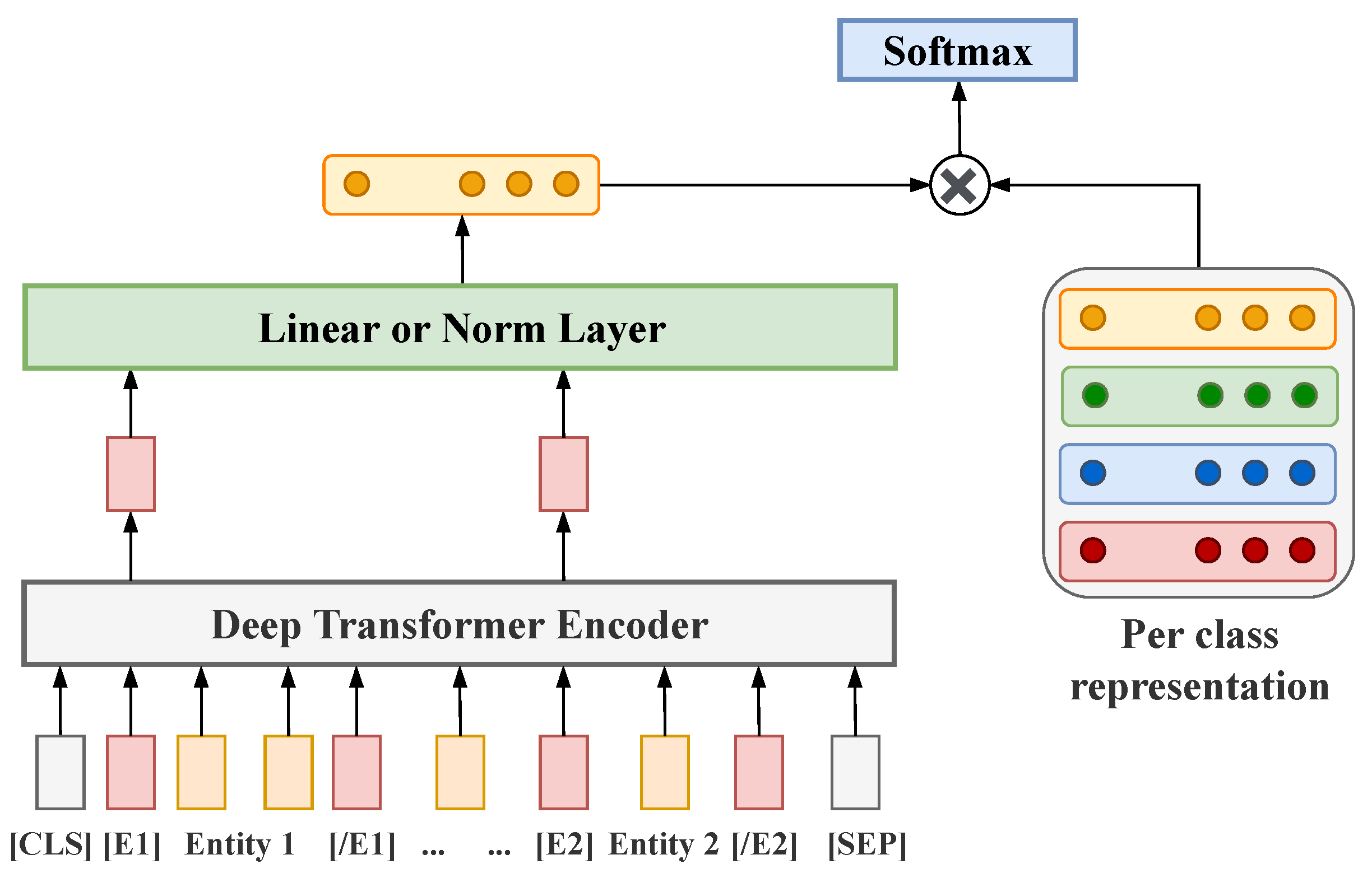
Standard approaches to supervised relation extraction that rely on deep neural networks usually encode the input sequence in terms of an attention layer to predict the type of relation between a specified pair of entities [61,62]. It is also common to introduce either mention pooling to perform classification only over encoded representations of entities or positional embeddings that indicate the tokens of the entities between which a relation holds in the input sequence to affect encoding itself [63,64,65]. In [24], the authors showed that special entity markers (functional tokens placed before and after the tokens of an entity) introduced into the token sequence instead of the traditional extra token type embedding layer lead to more accurate results. We adapt this model to our problem; cf. Figure 2.
The input to the model is a relation statement that contains a sequence of tokens x and the entity span identifiers and . Before introducing the sequence into the encoder, x is augmented by four reserved word pieces, , , , and , to mark the beginning and end of each entity mention in the relation statement as follows:
In addition, entity indices are updated to account for the inserted tokens: and . Given the last hidden layer of the transformer network defined as for , the concatenation of the final hidden states corresponding to the respective start entity markers is used to represent the relation in the encoder outcome: . It is worth noting that the authors of the model also tried two other items in the encoder outcome to be used for classification, namely, the CLS token and entity mention states, but concluded that the states corresponding to the start entity markers lead to the best scores. This representation is fed into a fully connected layer that either contains a linear activation or performs layer normalization [66]. The choice of the post Transformer layer is treated as a hyper-parameter. Furthermore, a classification layer is introduced, where H is the size of the relation representation and K is the number of relation types. The classification loss is the standard cross-entropy of the softmax of with respect to the true relation type.
5. Experiments
Extending the original G2C-Tr model by a dedicated relation-based collocation classification described above, we obtain a reinforced model architecture depicted in Figure 1, with two transformers dedicated specifically to collocation extraction and classification, respectively. In the follow-up experiments, we assess to what extent this extension leads to an improvement of the performance of the overall model.
In this section, we present the datasets that we used, the setup of the experiments, including the details of the training and the combination of the pre-trained models selected for each transformer block in Figure 1, and the results of the experiments.
5.1. Datasets
In order to be able to compare the performance of the extended model that we propose with the performance of the original G2C-Tr model [22], we use the same English, French, and Spanish datasets compiled from the 2019 Wikipedia dumps using the lists of LF instances of Fisas et al. [67] as seed lists. The dumps are preprocessed (removing metadata and markups) and parsed with the UDPipe2.5 (https://ufal.mff.cuni.cz/udpipe, accessed on 1 July 2022). From the parsed dumps, for each LF instance encountered in the lists of LF instances, sentences that contain this instance (with one of its valid dependency patterns) are extracted. Only those sentences are selected in which the lemmas of the base and collocate elements have the same PoS as specified in the list of LF instances compiled in [67]. In order to further minimize the number of the remaining erroneous samples in which the base and the collocate items do not form a collocation (as, e.g., in Conceding defeat, Cavaco Silva said he wished his rival “much success in meeting his duties for the good of all Portuguese”, where between success and meet an indirect dependency relation holds and the two words meet and success form, in principle, a collocation, but not in this sentence), an additional manual validation has been performed. For each LF and each syntactic dependency pattern between the base and the collocate elements of this LF, three sentences from the preliminary dataset are randomly picked. In case the base and the collocate elements did not form an instance of this LF, all sentences with the considered dependency pattern between the base and collocate elements were removed from the dataset (for this purpose, an expanded list of expected syntactic dependencies between the base and the collocate elements is used, namely, ‘acl’, ‘acl:relcl’, ‘advcl’, ‘advmod’, ‘amod’, ‘case’, ‘compound’, ‘conj’, ‘csubj’, ‘nmod’, ‘nsubj’, ‘nsubj:pass’, ‘obj’, ‘obl’, ‘obl:npmod’, and ‘xcomp’). This allowed us to take into account mistakes of the parser while not excluding correct examples with wrongly assigned dependencies). Table 2 displays the counts of the individual LF instances in the obtained English, French, and Spanish corpora.
The corpora are annotated with respect to the LF taxonomy and the sentence LF labels in terms of BI labels of the BIO sequence annotation schema for both elements of the instance, the base and the collocate (‘B-<LF>b’ and ‘I-<LF>b’ for the base, ‘B-<LF>c’, ‘I-<LF>c’ for the collocate, and ‘O’ for other tokens); see Figure 1 for an illustration. The BIO annotation has the advantage that it facilitates a convenient labeling of multi-word elements, and the separate annotation of the base and collocate elements allows for flawless annotation of cases where the base and the collocate elements are not adjacent. As a sentence label, the most frequent LF in a sentence and the first one in case of a draw is chosen.
For training of the relation classification transformer, we created an additional dataset, where we introduced entity markers into the input sequences ( for the base and for the collocate), such that the <LF> tag indicates the default order of the base and the collocate (e.g., in “Oper1(,)”, which is a verb–object construction, the verbal collocate precedes the base). In case one sentence contains several collocations, we use each of them for an individual training example by copying the sentence and introducing entity markers only for a single collocation at once. Thus, the number of examples is equal to the number of annotated collocations in our corpora. We did not introduce negative examples of any special “not-a-collocation” class to ensure that the transformer in extension cannot “cancel” a collocation extracted by the base G2C-Tr model but can only refine the lexical function assignment.
5.2. Setup of the Experiments
For the experiments, the obtained datasets were split into training, development, and test subsets in proportion 80–10–10 in terms of LF-wise unique instances, such that all occurrence samples of a single LF instance appear only in one of the subsets. Sentences with several collocations that belonged to different splits are dropped. Since collocations have different frequencies in the corpus, not each split leads to the same proportion in terms of overall number of samples. Therefore, for each LF, we additionally distributed collocations to ensure an approximate 80–10–10 split not only in terms of the number of LF instances in general but also in terms of the number of instances per LF.
In order to be able to clearly distinguish the contribution of our extension to the final figures, to run the experiments, we used the same versions of Transformers for the G2C-Tr model as in [22]: BERT-large (https://huggingface.co/bert-large-uncased, accessed on 1 July 2022) for English, XLM-RoBERTa-base (https://huggingface.co/xlm-roberta-base, accessed on 1 July 2022) for Spanish and French, and considered models trained with and without information about PoS tags.
As for the relation classification, we used different monolingual RoBERTa large and XLM-RoBERTa large-based models for English (https://huggingface.co/roberta-large, accessed on 1 July 2022), Spanish (https://huggingface.co/xlm-roberta-large, accessed on 1 July 2022), and French (https://huggingface.co/camembert/camembert-large, accessed on 1 July 2022). About 20% of the development set has been used for the evaluation of intermediate checkpoints during the training phase, and the three best checkpoints were evaluated on the entire development set in order to select the model to be used for the G2C-Tr extension. The batch size was of 16; the models were trained for 10 epochs (about 169,000 steps for English, 90,000 steps for Spanish, and 83,000 steps for French). Since, in contrast to the G2C-Tr base model, which may predict base without collocate and vise versa, our model extracts only complete collocations, we also removed unpaired B-I tags from the outcome of the base model and re-evaluated it to make the scores for both models comparable.
5.3. Results of the Experiments
In what follows, we first present the performance of the relation classification model with respect to the individual LFs and then show the results of the evaluation of the entire model, i.e., the extended G2C-Tr model.
Table 3, Table 4 and Table 5 provide precision (P), recall (R), and F1-scores (F1) achieved on the training, development and test set, respectively, per LF for each considered language (with ‘I’ as correctly identified instances of LF f, ‘A’ as all instances identified as instances of f, and ‘B’ as all instances of f in the test set, precision is defined as P = ∣I ∩ AA∣, recall as R = ∣A ∩ BB∣ and F1 as the harmonic mean of P and R: F1 = 2PR ∖ (P + R)). Within each LF, examples were split into two groups depending on the order of collocation parts in a sentence, i.e., when the collocate precedes the base () and when the base precedes the collocate (). The columns “#” show the number of examples in each group, with the total size of a set at the bottom.
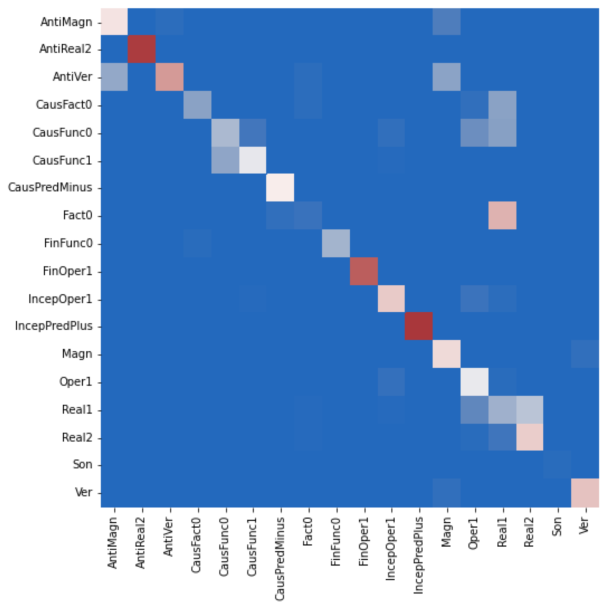
Table 6 reports the average F1-scores of (i) the original G2C-Tr model, i.e., for separate identification of the base and collocate elements across all LFs, without that both elements must have been identified; (ii) the original G2C-Tr model, but limited to cases when both elements are identified; (iii) the G2C-Tr model extended by the relation extraction layer. We provide the results for these three constellations because the first was used in [22] to report on the performance of the G2C-Tr model, while the second and third allow for a direct comparison between the original G2C-Tr model and the relation extraction-extended model. Configurations with an access to PoS embeddings (“G2C+PoS”) and without PoS embeddings (“G2C-PoS”) are assessed. Figure 3, Figure 4 and Figure 5 display the corresponding confusion matrices for the test set.
6. Discussion
Let us first discuss the performance of our relation extraction-based collocation classification model and then assess to what extent it contributes to the improvement of the basic G2C-Tr model.
6.1. Discussion of Relation Extraction-Based Collocation Classification
Already, a first cursory glance at Table 4 and Table 5 provides some interesting details on the grammatical constructions associated by our model with the instances of the individual LFs and thus also encountered in the corpora—sometimes in contrast to the expectations motivated by the canonical word order. For instance, the canonical word order in English and Spanish in adjective–noun LF instances is (), as, e.g., AntiMagn: low (=) temperature (=), Magn: high (=) temperature (=), Ver: comfort (=) temperature (=), and AntiVer: freezing (=) temperature (=). The model seems to learn both the canonical and the non-canonical orders rather well. It is to be noted, however, that for Magn in the English test set, the () pattern (as, e.g., in The temperatures were high) is recognized considerably better. For Ver, the same tendency can be identified, although by far not that clearly. For French, we see that in the case of AntiMagn, AntiVer, and Magn, the adjectives more often precede the noun, while for Ver, they follow the noun (most of the values are very close to 1.00 because we chose a checkpoint of the model generated at the moment when the model started being overfitted and the scores on the validation set stopped increasing). Especially for English, the canonical order of the collocation elements is also not reflected in the performance of the recognition of several verb–noun LFs. Thus, Oper1 and Real2 instances, which canonically instantiate the pattern (), show in Table 5 a better performance for (), and FinFunc0, which canonically instantiates the pattern (), shows a better performance for (). In Spanish and French, this “deviance” is observed to a much lesser degree. Since for English, it is also not observed that much on development data (Table 4), we may explain it by an insufficient number of different LF instances in our training data.
Table 4 and Table 5 also show a similar overall performance for English, French and Spanish, although the differences across the individual LFs are significant, ranging from an F1-score between 0.95 and 1.0 for the () pattern of FinFOper1 instances in English, French, and Spanish on both the development and test data to an F1-score between 0.01 and 0.95 for the pattern () of Real1. However, in general, we can conclude that our relation extraction-based model is able to capture various syntactic patterns of the LF instances.
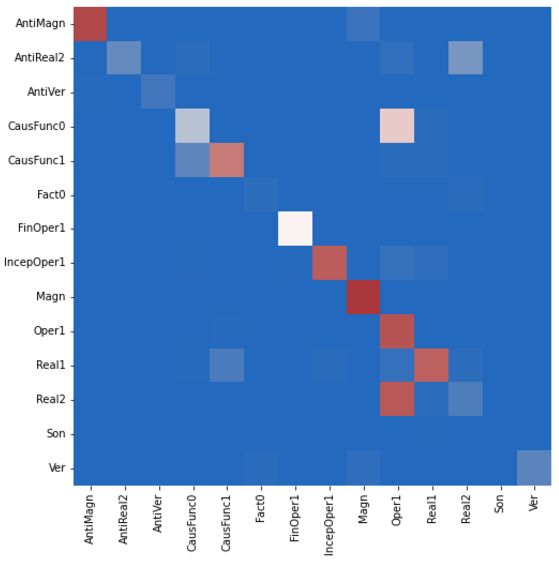
We cannot compare the performance of our model with the performance of other semantic classification models known from the literature (see Section 3) since they were trained and tested on other data; however, the confusion matrices in Figure 3, Figure 4 and Figure 5 suggest that our model does not confuse Magn with AntiMagn and only moderately AntiMagn with Magn LF instances and thus overcomes, like [22], the notorious problem of automatic distinction of antonyms. Furthermore, it practically does not confuse Magn and Ver instances, which is a challenge still experienced in [22].
Some semantically very similar LFs may still be confused. For instance, for English, CausFunc0 and CausFact0 can be confused with Real1 instances, and Real1 instances can be confused with Real2 instances. In general, the confusion matrices tell us that the model behaves similarly across languages, even if some language-specific confusion glitches can be observed; see also the analysis in [22] in this respect.
6.2. Does Relation Extraction Improve the Overall Performance of Collocation Classification?
The good performance of our relation extraction-driven collocation classification model as presented in Section 5.3 and discussed above legitimates its use as an extension of the G2C-Tr model to assess to what extent an explicit consideration of relation information helps in collocation recognition and classification. For this assessment, let us look at Table 6, which contrasts the results obtained with the basic G2C-Tr model with the performance of the G2C-Tr model extended by a relation extraction network. We can observe that the extension of the G2C-Tr model by a relation extraction network improves the classification performance of the original model when both elements of an LF instance have been identified before and when PoS information is taken into account. When PoS information is not considered, the performance of the original and the extended models are nearly the same for French and Spanish, while for English, the original model is better. Interestingly enough, for English, PoS information does not contribute to the performance, just on the contrary: a deeper linguistic analysis is needed to determine why this is the case.
Overall, we can conclude that for applications such as second language learning, for which a correct distinction between instances of semantically similar LFs is crucial (cf., e.g., Magn(voice) = loud vs. Ver(voice) = clear) or IncepOper1(war) = launch vs. Oper1(war) = wage), our extended model brings an advantage compared to the original G2C-Tr model. From the perspective of the research on neural collocation classification, we can state that the introduction of an additional explicit relation extraction network into a graph transformer-based collocation identification and classification model does not lead to a considerably higher classification performance. This confirms that when fed with syntactic dependencies between collocation elements in the training material, a graph transformer is also able to learn to a major extent the semantic relations between them, such that an additional explicit semantic relation extraction layer is of limited use only.
7. Conclusions and Future Work
Following the fact that between the elements of a collocation, i.e., a lexically restricted word co-occurrence, both a syntactic and a semantic dependency holds, we explored to what extent the addition of an explicit semantic relation extraction layer to a graph transformer model, which operates on syntactic dependencies, improves the overall performance of the identification and classification of collocations with respect to the LF taxonomy. Our experiments have shown that the Transformer is already able to capture the semantic relations and that although the additional relation extraction layer helps to somewhat improve the performance, this improvement is limited. It is also to be noted that the semantic relation extraction layer still does not fully solve the problem of the confusion of the instances of syntactically and/or semantically similar LFs, although an improvement compared to the original G2C-Tr model can be observed.
Along with these valuable newly gained insights, the presented work reveals some limitations. In particular to be mentioned is the fact that so far, the relation extraction model has been applied only to the task of classification of lexically restricted word co-occurrences. In our future work, we want to explore the potential of a relation extraction-based model for the joint identification and classification of LF instances.Furthermore, in our study, we did not pursue the question on how the exploitation of the information on syntactic sentence structures would influence the quality of the classification of LF instances with the canonical vs. non-canonical order of their elements. Finally, a more thorough linguistic analysis of the confusion matrices would certainly contribute to a better understanding and thus also to the solution of the classification of LF instances. It should be also clear to the reader that the number of different instances of certain LFs which are available so far for the training and fine-tuning of ML models is very limited. This restricts the potential of currently explored models (including the one presented in this work). To advance significantly, either novel models must be researched, which are able to learn (as humans do) on a few training data only, or substantially larger datasets need to be compiled.
Author Contributions
Conceptualization, A.S. and L.W.; methodology, A.S.; software, A.S.; validation, A.S. and L.W.; formal analysis, A.S.; investigation, A.S. and L.W.; resources, A.S. and L.W.; data curation, A.S. and L.W.; writing—original draft preparation, A.S. and L.W.; writing—review and editing, A.S. and L.W.; visualization, A.S.; supervision, L.W.; project administration, L.W.; funding acquisition, L.W. All authors have read and agreed to the published version of the manuscript.
Funding
This research was funded by the European Commission in the context of its H2020 Research and Development Program under the contract number 870930.
Data Availability Statement
All datasets are available upon request.
Acknowledgments
Many thanks to Luis Espinosa-Anke, Alireza Mohammadshahi, and James Henderson for the collaboration on the GrC-Tr model and to Beatriz Fisas, Alba Táboas and Inmaculada López for their contributions to the the original LF instance lists.
Conflicts of Interest
The authors declare no conflict of interest. The funders had no role in the design of the study, in the collection, analyses, or interpretation of data, in the writing of the manuscript, or in the decision to publish the results.
Abbreviations
The following abbreviations are used in this manuscript:
| BERT | Bidirectional Encoder Representation from Transformers |
| BIO | Begin-In-Out (tagging strategy) |
| CLS (token) | Special Classification Token (used in the BERT model) |
| F1 (score) | Harmonic mean between precision and recall |
| Gr2C | Graph-to-Collocation |
| Gr2C-Tr | Graph-to-Collocation Transformer |
| LF | Lexical Function |
| LVC | Light Verb Construction |
| ML | Machine Learning |
| NB | Naïve Bayes (machine learning technique) |
| NLP | Natural Language Processing |
| NN | Nearest Neighbour (machine learning technique) |
| P | Precision |
| PoS | Part of Speech |
| R | Recall |
| SLL | Second Language Learning |
| SVC | Support Verb Construction |
| TAN | Tree Augmented Network (machine learning technique) |
| UD | Universal Dependency |
References
- Hausmann, F.J. Wortschatzlernen ist Kollokationslernen. Zum Lehren und Lernen französischer Wortwendungen. Prax. Neusprachlichen Unterrichts 1984, 31, 395–406. [Google Scholar]
- Nation, I.S. Learning Vocabulary in Another Language; Ernst Klett Sprachen: Stuttgart, Germany, 2001. [Google Scholar]
- Nesselhauf, N. The Use of Collocations by Advanced Learners of English and Some Implications for Teaching. Appl. Linguist. 2003, 24, 223–242. [Google Scholar] [CrossRef] [Green Version]
- Lesniewska, J. Is cross-linguistic influence a factor in advanced EFL learners’ use of collocations. In Cross-Linguistic Influences in the Second Language Lexicon; Multilingual Matters: Clevedon, UK, 2006; pp. 65–77. [Google Scholar]
- Wang, Y.; Shaw, P. Transfer and Universality: Collocation Use in Advanced Chinese and Swedish Learner English. ICAME J. 2008, 32, 201–232. [Google Scholar]
- Wanner, L.; Verlinde, S.; Alonso Ramos, M. Writing assistants and automatic lexical error correction: Word combinatorics. In Proceedings of the eLex 2013 Conference, Tallinn, Estonia, 17–19 October 2013; Kosem, I., Kallas, J., Gantar, P., Krek, S., Langemets, M., Tuulik, M., Eds.; Trojina, Institute for Applied Slovene Studies & Eesti Keele Instituut: Tallinn, Estonia; Ljubljana, Slovenia, 2013; pp. 472–487. [Google Scholar]
- Smadja, F.; McKeown, K. Automatically Extracting and Representing Collocations for Language Generation. In Proceedings of the 28th Annual Meeting of the Association for Computational Linguistics, Pittsburgh, PA, USA, 6–9 June 1990; pp. 252–259. [Google Scholar]
- Wanner, L.; Bateman, J.A. A collocational based approach to salience sensitive lexical selection. In Proceedings of the 5th International Workshop on Natural Language Generation, Dawson, PA, USA, 3–6 June 1990. [Google Scholar]
- Seretan, V. On Collocations and their interaction with Parsing and Translation. Informatics 2014, 1, 11–31. [Google Scholar] [CrossRef] [Green Version]
- Scozzafava, F.; Maru, M.; Brignone, F.; Torrisi, G.; Navigli, R. Personalized PageRank with syntagmatic information for multilingual word sense disambiguation. In Proceedings of the 58th Annual Meeting of the Association for Computational Linguistics: System Demonstrations, Online, 5–10 July 2020; pp. 37–46. [Google Scholar]
- Maru, M.; Scozzafava, F.; Martelli, F.; Navigli, R. SyntagNet: Challenging supervised word sense disambiguation with lexical-semantic combinations. In Proceedings of the 2019 Conference on Empirical Methods in Natural Language Processing and the 9th International Joint Conference on Natural Language Processing (EMNLP-IJCNLP), Hong Kong, China, 3–7 November 2019; pp. 3525–3531. [Google Scholar]
- Mel’čuk, I.; Wanner, L. Lexical Functions and Lexical Inheritance for Emotion Lexemes in German. In Lexical Functions in Lexicography and Natural Language Processing; Wanner, L., Ed.; Benjamins Academic Publishers: Amsterdam, The Netherlands, 1996; pp. 209–278. [Google Scholar]
- Church, K.; Hanks, P. Word association norms, mutual information, and lexicography. Comput. Linguist. 1990, 16, 22–29. [Google Scholar]
- Bouma, G. Normalized (pointwise) mutual information in collocation extraction. Proc. GSCL 2009, 30, 31–40. [Google Scholar]
- Pecina, P. Lexical association measures and collocation extraction. Lang. Resour. Eval. 2010, 44, 137–158. [Google Scholar] [CrossRef]
- Wanner, L. Towards automatic fine-grained semantic classification of verb-noun collocations. Nat. Lang. Eng. 2004, 10, 95–143. [Google Scholar] [CrossRef]
- Wanner, L.; Bohnet, B.; Giereth, M. Making sense of collocations. Comput. Speech Lang. 2006, 20, 609–624. [Google Scholar] [CrossRef]
- Wanner, L.; Bohnet, B.; Giereth, M. What is beyond Collocations? Insights from Machine Learning Experiments. In Proceedings of the 12th Euralex International Congress on Lexicography (EURALEX), Torino, Italy, 6–9 September 2006; pp. 1071–1084. [Google Scholar]
- Espinosa-Anke, L.; Schockaert, S.; Wanner, L. Collocation classification with unsupervised relation vectors. In Proceedings of the 57th Annual Meeting of the Association for Computational Linguistics, Florence, Italy, 28 July–2 August 2019; pp. 5765–5772. [Google Scholar]
- Mel’čuk, I.A. Lexical Functions: A Tool for the Description of Lexical Relations in the Lexicon. In Lexical Functions in Lexicography and Natural Language Processing; Wanner, L., Ed.; Benjamins Academic Publishers: Amsterdam, The Netherlands, 1996; pp. 37–102. [Google Scholar]
- Wanner, L.; Ferraro, G.; Moreno, P. Towards Distributional Semantics-based Classification of Collocations for Collocation Dictionaries. Int. J. Lexicogr. 2017, 30, 167–186. [Google Scholar] [CrossRef]
- Espinosa-Anke, L.; Shvets, A.; Mohammadshah, A.; Henderson, J.; Wanner, L. Multilingual Extraction and Categorization of Lexical Collocations with Graph-aware Transformers. In Proceedings of the 57th Annual Meeting of the Association for Computational Linguistics, Florence, Italy, 28 July–2 August 2019; pp. 5765–5772. [Google Scholar]
- Ye, W.; Li, B.; Xie, R.; Sheng, Z.; Chen, L.; Zhang, S. Exploiting Entity BIO Tag Embeddings and Multi-task Learning for Relation Extraction with Imbalanced Data. In Proceedings of the 57th Annual Meeting of the Association for Computational Linguistics, Florence, Italy, 28 July–2 August 2019; pp. 1351–1360. [Google Scholar] [CrossRef]
- Soares, L.B.; Fitzgerald, N.; Ling, J.; Kwiatkowski, T. Matching the Blanks: Distributional Similarity for Relation Learning. In Proceedings of the 57th Annual Meeting of the Association for Computational Linguistics, Florence, Italy, 28 July–2 August 2019; pp. 2895–2905. [Google Scholar]
- Hausmann, F.J. Le dictionnaire de collocations. In Wörterbücher, Dictionaries, Dictionnaires: An international Handbook of Lexicography; Hausmann, F., Reichmann, O., Wiegand, H., Zgusta, L., Eds.; De Gruyter: Berlin, Germany; New York, NY, USA, 1989; pp. 1010–1019. [Google Scholar]
- Cowie, A.P. Phraseology. In The Encyclopedia of Language and Linguistics; Asher, R., Simpson, J., Eds.; Pergamon: Oxford, UK, 1994; Volume 6, pp. 3168–3171. [Google Scholar]
- Mel’čuk, I.A. Phrasemes in Language and Phraseology in Linguistics. In Idioms: Structural and Psychological Perspectives; Everaert, M., van der Linden, E.J., Schenk, A., Schreuder, R., Eds.; Lawrence Erlbaum Associates: Hillsdale, MI, USA, 1995; pp. 167–232. [Google Scholar]
- Kilgarriff, A. Collocationality (And How to Measure it). In Proceedings of the 12th Euralex International Congress on Lexicography (EURALEX), Torino, Italy, 6–9 September 2006; pp. 997–1004. [Google Scholar]
- Firth, J.R. Modes of Meaning. In Papers in Linguistics, 1934–1951; Firth, J., Ed.; Oxford University Press: Oxford, UK, 1957; pp. 190–215. [Google Scholar]
- Evens, M.W. Relational Models of the Lexicon: Representing Knowledge in Semantic Networks; Cambridge University Press: Cambridge, UK, 1988. [Google Scholar]
- Banarescu, L.; Bonial, C.; Cai, S.; Georgescu, M.; Griffitt, K.; Hermjakob, U.; Knight, K.; Koehn, P.; Palmer, M.; Schneider, N. Abstract Meaning Representation for Sembanking. In Proceedings of the 7th Linguistic Annotation Workshop and Interoperability with Discourse, Sofia, Bulgaria, 8–9 August 2013; pp. 178–186. [Google Scholar]
- Shwartz, V.; Dagan, I. Still a Pain in the Neck: Evaluating Text Representations on Lexical Composition. Trans. Assoc. Comput. Linguist. 2019, 7, 403–419. [Google Scholar] [CrossRef]
- Garcia, M.; Vieira, T.K.; Scarton, C.; Idiart, M.; Villavicencio, A. Probing for idiomaticity in vector space models. In Proceedings of the 16th Conference of the European Chapter of the Association for Computational Linguistics: Main Volume, Online, 19–23 April 2021; pp. 3551–3564. [Google Scholar]
- Choueka, Y. Looking for Needles in a Haystack or Locating Interesting Collocational Expressions in Large Textual Databases. In Proceedings of the 2nd International Conference on Computer-Assisted Information Retrieval (RIAO), Cambridge, MA, USA, 21–25 March 1988; pp. 34–38. [Google Scholar]
- Smadja, F. Retrieving Collocations from Text: X-Tract. Comput. Linguist. 1993, 19, 143–177. [Google Scholar]
- Carlini, R.; Codina-Filba, J.; Wanner, L. Improving collocation correction by ranking suggestions using linguistic knowledge. In Proceedings of the Third Workshop on NLP for Computer-Assisted Language Learning, Uppsala, Sweden, 13 November 2014; pp. 1–12. [Google Scholar]
- Dunning, T. Accurate Methods for the Statistics of Surprise and Coincidence. Comput. Linguist. 1993, 19, 61–74. [Google Scholar]
- Breidt, E. Extraction of N-V-collocations from text corpora: A feasibility study for German. In Proceedings of the 1st ACL Workshop on Very Large Corpora, Columbus, OH, USA, 22 June 1993. [Google Scholar]
- Pearce, D. A Comparative Evaluation of Collocation Extraction Techniques. In Proceedings of the Third International Conference on Language Resources and Evaluation (LREC’02), Las Palmas, Italy, 28 May–3 June 2002. [Google Scholar]
- Evert, S. Corpora and collocations. In Corpus Linguistics. An International Handbook; Lüdeling, A., Kytö, M., Eds.; Mouton de Gruyter: Berlin, Germany, 2008; pp. 1212–1248. [Google Scholar]
- Garcia, M.; Salido García, M.; Alonso Ramos, M. A comparison of statistical association measures for identifying dependency-based collocations in various languages. In Proceedings of the Joint Workshop on Multiword Expressions and WordNet (MWE-WN 2019), Florence, Italy, 2 August 2019; pp. 49–59. [Google Scholar]
- Krenn, B.; Evert, S. Can we do better than frequency? A case study on extracting PP-verb collocations. In Proceedings of the ACL Workshop on Collocations, Toulouse, France, 7 July 2001; pp. 39–46. [Google Scholar]
- Evert, S.; Krenn, B. Methods for the qualitative evaluation of lexical association measures. In Proceedings of the 39th Annual Meeting of the Association for Computational Linguistics, Toulouse, France, 9–11 July 2001; pp. 188–195. [Google Scholar]
- Heid, U.; Raab, S. Collocations in multilingual generation. In Proceedings of the Fourth Conference of the European Chapter of the Association for Computational Linguistics, Manchester, UK, 10–12 April 1989. [Google Scholar]
- Lin, D. Automatic identification of non-compositional phrases. In Proceedings of the 37th Annual Meeting of the Association for Computational Linguistics, College Park, MD, USA, 20–26 June 1999; pp. 317–324. [Google Scholar]
- Seretan, V.; Wehrli, E. Accurate collocation extraction using a multilingual parser. In Proceedings of the 21st International Conference on Computational Linguistics and 44th Annual Meeting of the Association for Computational Linguistics, Sydney, Australia, 17–18 July 2006; pp. 953–960. [Google Scholar]
- Dras, M. Automatic Identification of Support Verbs: A Step Towards a Definition of Semantic Weight. In Proceedings of the Eighth Australian Joint Conference on Artificial Intelligence, Canberra, Australia, 13–17 November 1995; pp. 451–458. [Google Scholar]
- Vincze, V.; Nagy, I.; Zsibrita, J. Learning to detect English and Hungarian light verb constructions. ACM Trans. Speech Lang. Process. 2013, 10, 1–25. [Google Scholar] [CrossRef]
- Kettnerová, V.; Lopatková, M.; Bejček, E.; Vernerová, A.; Podobová, M. Corpus Based Identification of Czech Light Verbs. In Proceedings of the Seventh International Conference Slovko, Natural Language Processing, Corpus Linguistics, E-Learning, Bratislava, Slovakia, 13–15 November 2013; RAM Verlag: Lüdenscheid, Germany, 2013; pp. 118–128. [Google Scholar]
- Chen, W.T.; Bonial, C.; Palmer, M. English Light Verb Construction Identification Using Lexical Knowledge. In Proceedings of the Twenty-Ninth AAAI Conference on Artificial Intelligence, Phoenix, AZ, USA, 12–17 February 2016; pp. 2375–2381. [Google Scholar]
- Cordeiro, S.R.; Candito, M. Syntax-based identification of light-verb construc- tions. In Proceedings of the 22nd Nordic Conference on Computational Linguistics, Turku, Finland, 30 September–2 October 2019; pp. 97–104. [Google Scholar]
- Huang, C.C.; Kao, K.H.; Tseng, C.H.; Chang, J.S. A Thesaurus-Based Semantic Classification of English Collocations. Comput. Linguist. Chin. Lang. Process. 2009, 14, 257–280. [Google Scholar]
- Vossen, P. EuroWordNet: A Multilingual Database with Lexical Semantic Networks; Kluwer Academic Publishers: Dordrecht, The Netherlands, 1998. [Google Scholar]
- Gelbukh, A.; Kolesnikova, O. Semantic Analysis of Verbal Collocations with Lexical Functions; Springer: Cham, Switzerland, 2012; Volume 414. [Google Scholar]
- Orliac, B.; Dillinger, M. Collocation extraction for machine translation. In Proceedings of the Machine Translation Summit IX: Papers, New Orleans, LA, USA, 23–27 September 2003. [Google Scholar]
- Baldwin, T. Looking for Prepositional Verbs in Corpus Data. In Proceedings of the 2nd ACL-SIGSEM Workshop on the Linguistic Dimensions of Prepositions and their Use in Computational Linguistics Formalisms and Applications, Colchester, UK, 19–21 April 2005. [Google Scholar]
- Rodríguez-Fernández, S.; Carlini, R.; Espinosa-Anke, L.; Wanner, L. Example-based Acquisition of Fine-grained Collocation Resources. In Proceedings of the Tenth International Conference on Language Resources and Evaluation, Portorož, Slovenia, 23–28 May 2016. [Google Scholar]
- Rodríguez Fernández, S.; Espinosa-Anke, L.; Carlini, R.; Wanner, L. Semantics-driven recognition of collocations using word embeddings. In Proceedings of the 54th Annual Meeting of the Association for Computational Linguistics, Berlin, Germany, 7–12 August 2016; pp. 499–505. [Google Scholar]
- Sanh, V.; Wolf, T.; Ruder, S. A hierarchical multi-task approach for learning embeddings from semantic tasks. In Proceedings of the AAAI Conference on Artificial Intelligence, Honolulu, HI, USA, 27 January–1 February 2019; Volume 33, pp. 6949–6956. [Google Scholar]
- Vaswani, A.; Shazeer, N.; Parmar, N.; Uszkoreit, J.; Jones, L.; Gomez, A.N.; Kaiser, Ł.; Polosukhin, I. Attention is all you need. In Proceedings of the Advances in Neural Information Processing Systems, Long Beach, CA, USA, 4–9 December 2017; pp. 5998–6008.
- Wang, L.; Cao, Z.; De Melo, G.; Liu, Z. Relation classification via multi-level attention cnns. In Proceedings of the 54th Annual Meeting of the Association for Computational Linguistics (Volume 1: Long Papers), Berlin, Germany, 7–12 August 2016; pp. 1298–1307. [Google Scholar]
- Lin, Y.; Shen, S.; Liu, Z.; Luan, H.; Sun, M. Neural relation extraction with selective attention over instances. In Proceedings of the 54th Annual Meeting of the Association for Computational Linguistics (Volume 1: Long Papers), Berlin, Germany, 7–12 August 2016; pp. 2124–2133. [Google Scholar]
- Zhang, Y.; Zhong, V.; Chen, D.; Angeli, G.; Manning, C.D. Position-aware attention and supervised data improve slot filling. In Proceedings of the Conference on Empirical Methods in Natural Language Processing, Copenhagen, Denmark, 7–11 September 2017. [Google Scholar]
- Bilan, I.; Roth, B. Position-aware self-attention with relative positional encodings for slot filling. arXiv 2018, arXiv:1807.03052. [Google Scholar]
- Nguyen, T.N.; Dernoncourt, F.; Nguyen, T.H. On the Effectiveness of the Pooling Methods for Biomedical Relation Extraction with Deep Learning. In Proceedings of the Tenth International Workshop on Health Text Mining and Information Analysis (LOUHI 2019), Hong Kong, China, 3–4 November 2019; pp. 18–27. [Google Scholar]
- Ba, J.L.; Kiros, J.R.; Hinton, G.E. Layer normalization. arXiv 2016, arXiv:1607.06450. [Google Scholar]
- Fisas, B.; Espinosa Anke, L.; Codina-Filbá, J.; Wanner, L. CollFrEn: Rich Bilingual English–French Collocation Resource. In Proceedings of the Joint Workshop on Multiword Expressions and Electronic Lexicons, Online, 3 December 2020; pp. 1–12. [Google Scholar]
Figure 1.
Relation-Based Graph-to-Collocation Transformer.

Figure 2.
Relation-Based Collocation Classification.

Figure 3.
Confusion matrix for the classification of all LFs by our relation model on the English test set.
Figure 3.
Confusion matrix for the classification of all LFs by our relation model on the English test set.

Figure 4.
Confusion matrix for the classification of all LFs by our relation model on the Spanish test set.
Figure 4.
Confusion matrix for the classification of all LFs by our relation model on the Spanish test set.

Figure 5.
Confusion matrix for the classification of all LFs by our relation model on the French test set.
Figure 5.
Confusion matrix for the classification of all LFs by our relation model on the French test set.


Table 1.
LF relations used in this paper. ‘A’ refers to AMR argument labels [31].
Table 1.
LF relations used in this paper. ‘A’ refers to AMR argument labels [31].
| Relation | Example | LF Label |
|---|---|---|
| intense | major∼strike | Magn |
| minor | selective∼strike | AntiMagn |
| genuine | legitimate∼strike | Ver |
| non-genuine | illegal∼strike | AntiVer |
| Increase.existence | fire∼spread | IncepPredPlus |
| End.existence | fire∼go out | FinFunc0 |
| A0.Come.to.effect | fire∼gut | Fact0 |
| A0/A1.Cause.existence | raise∼hope | CausFunc0 |
| A0/A1.Cause.function | start∼engine | CausFact0 |
| Cause.decrease | relieve∼tension | CausPredMinus |
| A0/A1.Cause.involvement | raisehope [in] | CausFunc1 |
| Emit.sound | elephant∼trumpet | Son |
| A0/A1.act | lend∼support | Oper1 |
| A0/A1.begin.act | gain∼impression | IncepOper1 |
| A0.end.act | withdraw∼support | FinOper1 |
| A0/A1.Act.acc.expectation | prove∼accusation | Real1 |
| A2.Act.acc.expectation | enjoy∼support | Real2 |
| A2.Act.x.expectation | betray∼trust | AntiReal2 |
Table 2.
Number of collocations, in total (tot.) and unique (un.), in the datasets across the LFs.
| English | French | Spanish | ||||||||||
|---|---|---|---|---|---|---|---|---|---|---|---|---|
| Train | Dev/Test | Train | Dev/Test | Train | Dev/Test | |||||||
| LF | tot. | un. | tot. | un. | tot. | un. | tot. | un. | tot. | un. | tot. | un. |
| Magn | 12,704 | 869 | 1681 | 100 | 15,131 | 541 | 1885 | 64 | 15,031 | 475 | 1751 | 55 |
| Oper1 | 11,381 | 577 | 1328 | 68 | 14,906 | 583 | 1902 | 68 | 14,781 | 369 | 1733 | 44 |
| Real1 | 14,052 | 184 | 1934 | 21 | 14,838 | 148 | 2049 | 18 | 15,059 | 48 | 1981 | 6 |
| AntiMagn | 15,067 | 170 | 1854 | 20 | 14,818 | 101 | 1854 | 12 | 15,240 | 96 | 1930 | 12 |
| IncepOper1 | 14,176 | 139 | 1846 | 17 | 14,984 | 131 | 1964 | 16 | 15,113 | 88 | 1882 | 11 |
| CausFunc1 | 15,016 | 70 | 1876 | 8 | 15,251 | 68 | 1853 | 8 | 14,998 | 44 | 2032 | 6 |
| CausFunc0 | 14,788 | 90 | 1892 | 12 | 15,176 | 99 | 1947 | 12 | 15,240 | 63 | 1868 | 8 |
| Real2 | 14,658 | 89 | 1926 | 11 | 12,454 | 47 | 3370 | 6 | 4255 | 9 | 497 | 1 |
| FinOper1 | 19,141 | 40 | 2613 | 5 | 8066 | 29 | 1014 | 4 | 6656 | 19 | 780 | 3 |
| AntiReal2 | 22,303 | 77 | 2866 | 9 | 5008 | 42 | 672 | 5 | 5369 | 40 | 683 | 5 |
| AntiVer | 25,998 | 136 | 3315 | 17 | 876 | 26 | 108 | 3 | 5805 | 61 | 704 | 8 |
| IncepPredPlus | 22,538 | 61 | 2897 | 7 | 0 | 0 | 0 | 0 | 4869 | 19 | 571 | 3 |
| CausPredMinus | 13,589 | 49 | 1106 | 6 | 0 | 0 | 0 | 0 | 4485 | 29 | 540 | 4 |
| Fact0 | 16,755 | 45 | 2138 | 5 | 388 | 11 | 28 | 2 | 1877 | 17 | 235 | 2 |
| Ver | 14,093 | 86 | 1893 | 11 | 2115 | 40 | 257 | 5 | 284 | 13 | 36 | 2 |
| CausFact0 | 10,438 | 39 | 1338 | 5 | 0 | 0 | 0 | 0 | 5102 | 18 | 643 | 3 |
| Son | 195 | 36 | 42 | 5 | 125 | 22 | 15 | 3 | 0 | 0 | 0 | 0 |
| FinFunc0 | 4740 | 20 | 504 | 3 | 0 | 0 | 0 | 0 | 274 | 4 | 69 | 1 |
| Total | 261,632 | 2777 | 33,049 | 330 | 134,136 | 1888 | 18,918 | 226 | 144,438 | 1412 | 17,935 | 174 |
Table 3.
Results breakdown per LF on the training set, where, for each LF, we list individual results for different order of bases and collocates in a sentence.
Table 3.
Results breakdown per LF on the training set, where, for each LF, we list individual results for different order of bases and collocates in a sentence.
| EN | ES | FR | ||||||||||
|---|---|---|---|---|---|---|---|---|---|---|---|---|
| P | R | F1 | # | P | R | F1 | # | P | R | F1 | # | |
| AntiMagn | 1.00 | 1.00 | 1.00 | 14,600 | 1.00 | 1.00 | 1.00 | 8772 | 1.00 | 1.00 | 1.00 | 9664 |
| AntiMagn | 1.00 | 1.00 | 1.00 | 576 | 1.00 | 1.00 | 1.00 | 6468 | 1.00 | 1.00 | 1.00 | 5154 |
| AntiReal2 | 1.00 | 1.00 | 1.00 | 19,180 | 1.00 | 1.00 | 1.00 | 4899 | 1.00 | 1.00 | 1.00 | 4128 |
| AntiReal2 | 1.00 | 1.00 | 1.00 | 3232 | 1.00 | 0.99 | 0.99 | 470 | 1.00 | 1.00 | 1.00 | 880 |
| AntiVer | 1.00 | 1.00 | 1.00 | 23,600 | 1.00 | 1.00 | 1.00 | 1435 | 1.00 | 0.98 | 0.99 | 50 |
| AntiVer | 1.00 | 1.00 | 1.00 | 2534 | 1.00 | 1.00 | 1.00 | 4370 | 1.00 | 1.00 | 1.00 | 826 |
| CausFact0 | 1.00 | 1.00 | 1.00 | 7900 | 0.98 | 1.00 | 0.99 | 4638 | - | - | - | - |
| CausFact0 | 1.00 | 1.00 | 1.00 | 2612 | 0.99 | 0.98 | 0.99 | 464 | - | - | - | - |
| CausFunc0 | 1.00 | 1.00 | 1.00 | 10,005 | 0.98 | 0.99 | 0.98 | 12,754 | 1.00 | 1.00 | 1.00 | 8978 |
| CausFunc0 | 1.00 | 0.99 | 0.99 | 5032 | 0.98 | 0.99 | 0.99 | 2486 | 1.00 | 1.00 | 1.00 | 6198 |
| CausFunc1 | 1.00 | 1.00 | 1.00 | 12,730 | 0.95 | 0.98 | 0.96 | 12,572 | 1.00 | 1.00 | 1.00 | 11,892 |
| CausFunc1 | 0.98 | 0.99 | 0.99 | 2452 | 1.00 | 0.98 | 0.99 | 2426 | 1.00 | 1.00 | 1.00 | 3359 |
| CausPredMinus | 1.00 | 1.00 | 1.00 | 11,599 | 1.00 | 1.00 | 1.00 | 3618 | - | - | - | - |
| CausPredMinus | 1.00 | 1.00 | 1.00 | 2162 | 0.99 | 1.00 | 1.00 | 867 | - | - | - | - |
| Fact0 | 0.99 | 1.00 | 1.00 | 5078 | 0.88 | 0.93 | 0.91 | 724 | 1.00 | 1.00 | 1.00 | 5 |
| Fact0 | 1.00 | 1.00 | 1.00 | 11,877 | 1.00 | 0.95 | 0.98 | 1153 | 1.00 | 1.00 | 1.00 | 383 |
| FinFunc0 | 1.00 | 1.00 | 1.00 | 4755 | 1.00 | 0.99 | 0.99 | 179 | - | - | - | - |
| FinFunc0 | 1.00 | 1.00 | 1.00 | 13 | 1.00 | 1.00 | 1.00 | 95 | - | - | - | - |
| FinOper1 | 1.00 | 1.00 | 1.00 | 18,941 | 1.00 | 0.99 | 1.00 | 6513 | 1.00 | 1.00 | 1.00 | 7728 |
| FinOper1 | 0.99 | 1.00 | 0.99 | 375 | 0.99 | 1.00 | 1.00 | 143 | 1.00 | 1.00 | 1.00 | 338 |
| IncepOper1 | 1.00 | 1.00 | 1.00 | 14,223 | 0.99 | 1.00 | 0.99 | 14,193 | 1.00 | 1.00 | 1.00 | 13,825 |
| IncepOper1 | 0.98 | 0.99 | 0.99 | 633 | 0.98 | 0.99 | 0.99 | 920 | 1.00 | 1.00 | 1.00 | 1159 |
| IncepPredPlus | 1.00 | 1.00 | 1.00 | 16,328 | 1.00 | 1.00 | 1.00 | 3502 | - | - | - | - |
| IncepPredPlus | 1.00 | 1.00 | 1.00 | 6496 | 1.00 | 1.00 | 1.00 | 1367 | - | - | - | - |
| Magn | 1.00 | 1.00 | 1.00 | 13,467 | 1.00 | 1.00 | 1.00 | 12,089 | 1.00 | 1.00 | 1.00 | 10,021 |
| Magn | 1.00 | 0.99 | 0.99 | 997 | 1.00 | 0.99 | 1.00 | 2942 | 1.00 | 1.00 | 1.00 | 5110 |
| Oper1 | 0.99 | 1.00 | 1.00 | 11,989 | 1.00 | 0.97 | 0.98 | 13,166 | 1.00 | 0.97 | 0.98 | 14,458 |
| Oper1 | 0.99 | 1.00 | 0.99 | 2630 | 1.00 | 0.98 | 0.99 | 1615 | 1.00 | 0.99 | 0.99 | 448 |
| Real1 | 1.00 | 1.00 | 1.00 | 13,895 | 1.00 | 0.99 | 0.99 | 12,147 | 0.96 | 1.00 | 0.98 | 11,431 |
| Real1 | 1.00 | 0.99 | 1.00 | 1103 | 0.98 | 1.00 | 0.99 | 2912 | 1.00 | 1.00 | 1.00 | 3407 |
| Real2 | 1.00 | 1.00 | 1.00 | 14,090 | 1.00 | 1.00 | 1.00 | 4213 | 1.00 | 1.00 | 1.00 | 11,537 |
| Real2 | 1.00 | 1.00 | 1.00 | 1100 | 1.00 | 1.00 | 1.00 | 42 | 1.00 | 1.00 | 1.00 | 917 |
| Son | 0.99 | 0.99 | 0.99 | 74 | - | - | - | - | 0.94 | 0.94 | 0.94 | 17 |
| Son | 1.00 | 0.99 | 1.00 | 130 | - | - | - | - | 1.00 | 1.00 | 1.00 | 108 |
| Ver | 1.00 | 1.00 | 1.00 | 13,365 | 0.96 | 0.87 | 0.91 | 30 | 1.00 | 0.99 | 1.00 | 334 |
| Ver | 0.99 | 1.00 | 1.00 | 1396 | 1.00 | 1.00 | 1.00 | 254 | 1.00 | 1.00 | 1.00 | 1781 |
| macro avg | 1.00 | 1.00 | 1.00 | 271,169 | 0.99 | 0.99 | 0.99 | 144,438 | 1.00 | 0.99 | 1.00 | 134,136 |
| weighted avg | 1.00 | 1.00 | 1.00 | 271,169 | 0.99 | 0.99 | 0.99 | 144,438 | 1.00 | 1.00 | 1.00 | 134,136 |
Table 4.
Results breakdown per LF on the development set, where, for each LF, we list individual results for different order of bases and collocates in a sentence.
Table 4.
Results breakdown per LF on the development set, where, for each LF, we list individual results for different order of bases and collocates in a sentence.
| EN | ES | FR | ||||||||||
|---|---|---|---|---|---|---|---|---|---|---|---|---|
| P | R | F1 | # | P | R | F1 | # | P | R | F1 | # | |
| AntiMagn | 0.97 | 0.99 | 0.98 | 1871 | 1.00 | 1.00 | 1.00 | 1475 | 1.00 | 0.99 | 0.99 | 1000 |
| AntiMagn | 0.80 | 1.00 | 0.89 | 40 | 0.98 | 0.92 | 0.95 | 347 | 0.99 | 0.97 | 0.98 | 728 |
| AntiReal2 | 1.00 | 0.98 | 0.99 | 2817 | 1.00 | 0.89 | 0.94 | 598 | 0.91 | 1.00 | 0.95 | 618 |
| AntiReal2 | 1.00 | 0.95 | 0.97 | 133 | 1.00 | 0.91 | 0.95 | 96 | 0.90 | 0.99 | 0.94 | 82 |
| AntiVer | 1.00 | 0.93 | 0.96 | 3052 | 1.00 | 0.99 | 0.99 | 93 | 1.00 | 1.00 | 1.00 | 40 |
| AntiVer | 0.99 | 0.85 | 0.91 | 190 | 0.98 | 0.95 | 0.96 | 600 | 0.97 | 0.53 | 0.69 | 64 |
| CausFact0 | 0.79 | 0.38 | 0.52 | 846 | 0.81 | 0.60 | 0.69 | 485 | - | - | - | - |
| CausFact0 | 0.46 | 0.08 | 0.13 | 550 | 0.97 | 0.56 | 0.71 | 112 | - | - | - | - |
| CausFunc0 | 0.89 | 0.17 | 0.29 | 1666 | 0.91 | 0.30 | 0.45 | 1502 | 0.76 | 0.15 | 0.25 | 1376 |
| CausFunc0 | 0.75 | 0.27 | 0.40 | 150 | 0.99 | 0.63 | 0.77 | 317 | 0.96 | 0.85 | 0.91 | 628 |
| CausFunc1 | 0.74 | 0.98 | 0.84 | 1743 | 0.79 | 0.99 | 0.87 | 1934 | 0.91 | 0.91 | 0.91 | 1418 |
| CausFunc1 | 0.82 | 0.92 | 0.87 | 112 | 0.52 | 0.95 | 0.67 | 109 | 0.95 | 0.93 | 0.94 | 389 |
| CausPredMinus | 0.99 | 1.00 | 0.99 | 660 | 0.92 | 0.98 | 0.95 | 440 | - | - | - | - |
| CausPredMinus | 1.00 | 1.00 | 1.00 | 43 | 0.98 | 0.87 | 0.92 | 63 | - | - | - | - |
| Fact0 | 0.86 | 0.72 | 0.79 | 1160 | 0.25 | 0.44 | 0.32 | 102 | - | - | - | - |
| Fact0 | 0.60 | 0.72 | 0.65 | 1060 | 0.62 | 0.56 | 0.59 | 136 | 0.71 | 1.00 | 0.83 | 10 |
| FinFunc0 | 0.95 | 0.98 | 0.96 | 210 | 0.50 | 0.84 | 0.62 | 75 | - | - | - | - |
| FinFunc0 | 0.00 | 0.00 | 0.00 | 3 | 0.47 | 1.00 | 0.64 | 34 | - | - | - | - |
| FinOper1 | 1.00 | 1.00 | 1.00 | 2688 | 0.99 | 0.91 | 0.95 | 716 | 1.00 | 1.00 | 1.00 | 919 |
| FinOper1 | 1.00 | 1.00 | 1.00 | 11 | 0.31 | 0.17 | 0.22 | 30 | 0.99 | 1.00 | 0.99 | 81 |
| IncepOper1 | 0.95 | 0.88 | 0.92 | 1678 | 0.77 | 0.96 | 0.86 | 1744 | 0.88 | 0.99 | 0.93 | 1812 |
| IncepOper1 | 0.68 | 0.82 | 0.74 | 82 | 0.83 | 0.85 | 0.84 | 164 | 0.88 | 0.98 | 0.93 | 204 |
| IncepPredPlus | 1.00 | 1.00 | 1.00 | 2375 | 0.87 | 0.99 | 0.93 | 351 | - | - | - | - |
| IncepPredPlus | 1.00 | 1.00 | 1.00 | 628 | 0.97 | 0.98 | 0.98 | 196 | - | - | - | - |
| Magn | 0.97 | 1.00 | 0.98 | 1613 | 0.97 | 0.99 | 0.98 | 1454 | 0.98 | 0.95 | 0.97 | 758 |
| Magn | 0.90 | 0.96 | 0.93 | 112 | 0.86 | 0.90 | 0.88 | 258 | 0.96 | 0.99 | 0.98 | 1012 |
| Oper1 | 0.51 | 0.91 | 0.66 | 1137 | 0.51 | 0.97 | 0.67 | 1495 | 0.48 | 0.85 | 0.62 | 1868 |
| Oper1 | 0.43 | 0.73 | 0.54 | 283 | 0.67 | 0.97 | 0.79 | 256 | 0.18 | 0.97 | 0.30 | 73 |
| Real1 | 0.56 | 0.81 | 0.66 | 1837 | 0.95 | 0.35 | 0.51 | 1840 | 0.97 | 0.59 | 0.73 | 1472 |
| Real1 | 0.01 | 0.03 | 0.01 | 116 | 0.68 | 0.51 | 0.58 | 106 | 0.90 | 0.51 | 0.65 | 620 |
| Real2 | 0.76 | 0.67 | 0.71 | 1587 | 1.00 | 0.94 | 0.97 | 464 | 1.00 | 1.00 | 1.00 | 4604 |
| Real2 | 0.67 | 0.47 | 0.55 | 378 | - | - | - | - | 0.71 | 0.74 | 0.73 | 139 |
| Son | 1.00 | 0.45 | 0.62 | 11 | - | - | - | - | 0.00 | 0.00 | 0.00 | 1 |
| Son | 1.00 | 0.98 | 0.99 | 44 | - | - | - | - | 0.91 | 0.71 | 0.80 | 14 |
| Ver | 0.94 | 1.00 | 0.97 | 1333 | 0.00 | 0.00 | 0.00 | 29 | 0.03 | 0.25 | 0.05 | 4 |
| Ver | 0.96 | 1.00 | 0.98 | 596 | 0.00 | 0.00 | 0.00 | 7 | 1.00 | 0.95 | 0.97 | 257 |
| macro avg | 0.80 | 0.77 | 0.76 | 32,815 | 0.76 | 0.75 | 0.73 | 17,628 | 0.81 | 0.81 | 0.78 | 20,191 |
| weighted avg | 0.87 | 0.84 | 0.83 | 32,815 | 0.86 | 0.81 | 0.80 | 17,628 | 0.90 | 0.86 | 0.85 | 20,191 |
Table 5.
Results breakdown per LF on the test set, where, for each LF, we list individual results for different order of bases and collocates in a sentence.
Table 5.
Results breakdown per LF on the test set, where, for each LF, we list individual results for different order of bases and collocates in a sentence.
| EN | ES | FR | ||||||||||
|---|---|---|---|---|---|---|---|---|---|---|---|---|
| P | R | F1 | # | P | R | F1 | # | P | R | F1 | # | |
| AntiMagn | 0.70 | 0.87 | 0.77 | 1747 | 1.00 | 0.94 | 0.97 | 1105 | 1.00 | 1.00 | 1.00 | 1724 |
| AntiMagn | 0.95 | 0.91 | 0.93 | 67 | 0.96 | 0.83 | 0.89 | 933 | 0.91 | 0.72 | 0.80 | 255 |
| AntiReal2 | 1.00 | 1.00 | 1.00 | 2291 | 0.93 | 0.99 | 0.96 | 504 | 1.00 | 0.44 | 0.61 | 446 |
| AntiReal2 | 1.00 | 1.00 | 1.00 | 486 | 0.70 | 1.00 | 0.82 | 167 | 0.98 | 0.25 | 0.40 | 198 |
| AntiVer | 0.98 | 0.74 | 0.84 | 2700 | 0.67 | 0.50 | 0.57 | 8 | - | - | - | - |
| AntiVer | 0.96 | 0.16 | 0.27 | 683 | 0.94 | 0.65 | 0.77 | 707 | 0.99 | 0.86 | 0.92 | 111 |
| CausFact0 | 0.93 | 0.37 | 0.53 | 1007 | 0.12 | 0.03 | 0.05 | 659 | - | - | - | - |
| CausFact0 | 0.97 | 0.76 | 0.85 | 280 | 0.00 | 0.00 | 0.00 | 29 | - | - | - | - |
| CausFunc0 | 0.56 | 0.43 | 0.49 | 1804 | 0.98 | 0.46 | 0.63 | 1616 | 0.85 | 0.29 | 0.44 | 1545 |
| CausFunc0 | 0.86 | 0.21 | 0.33 | 174 | 1.00 | 0.11 | 0.20 | 300 | 0.48 | 0.52 | 0.50 | 344 |
| CausFunc1 | 0.87 | 0.61 | 0.72 | 1602 | 0.96 | 0.43 | 0.59 | 1888 | 0.93 | 0.96 | 0.94 | 1567 |
| CausFunc1 | 0.98 | 0.89 | 0.94 | 276 | 1.00 | 0.39 | 0.56 | 133 | 0.80 | 0.42 | 0.55 | 331 |
| CausPredMinus | 0.96 | 1.00 | 0.98 | 1304 | 1.00 | 1.00 | 1.00 | 450 | - | - | - | - |
| CausPredMinus | 0.98 | 1.00 | 0.99 | 201 | 1.00 | 0.99 | 1.00 | 126 | - | - | - | - |
| Fact0 | 0.32 | 0.04 | 0.08 | 337 | 0.00 | 0.00 | 0.00 | 45 | - | - | - | - |
| Fact0 | 0.54 | 0.05 | 0.09 | 1728 | 0.41 | 0.12 | 0.19 | 186 | 0.69 | 0.59 | 0.64 | 46 |
| FinFunc0 | 0.99 | 0.96 | 0.98 | 791 | 0.30 | 1.00 | 0.47 | 14 | - | - | - | - |
| FinFunc0 | 0.00 | 0.00 | 0.00 | 4 | 0.42 | 1.00 | 0.60 | 14 | - | - | - | - |
| FinOper1 | 1.00 | 1.00 | 1.00 | 2498 | 1.00 | 0.99 | 0.99 | 794 | 0.99 | 1.00 | 0.99 | 906 |
| FinOper1 | 1.00 | 1.00 | 1.00 | 27 | 0.27 | 0.95 | 0.42 | 20 | 0.99 | 1.00 | 1.00 | 121 |
| IncepOper1 | 0.91 | 0.92 | 0.91 | 1687 | 0.61 | 0.84 | 0.71 | 1778 | 0.99 | 0.93 | 0.96 | 1721 |
| IncepOper1 | 0.88 | 0.82 | 0.85 | 253 | 0.79 | 0.76 | 0.77 | 78 | 0.99 | 0.97 | 0.98 | 190 |
| IncepPredPlus | 1.00 | 1.00 | 1.00 | 1842 | 0.78 | 0.99 | 0.87 | 359 | - | - | - | - |
| IncepPredPlus | 0.99 | 1.00 | 1.00 | 968 | 1.00 | 1.00 | 1.00 | 235 | - | - | - | - |
| Magn | 0.84 | 0.96 | 0.90 | 1593 | 0.89 | 1.00 | 0.94 | 966 | 1.00 | 1.00 | 1.00 | 1506 |
| Magn | 0.16 | 0.94 | 0.27 | 112 | 0.48 | 1.00 | 0.65 | 823 | 0.82 | 0.98 | 0.89 | 493 |
| Oper1 | 0.56 | 0.92 | 0.70 | 1100 | 0.43 | 0.86 | 0.57 | 1476 | 0.39 | 0.99 | 0.56 | 1722 |
| Oper1 | 0.64 | 0.95 | 0.77 | 237 | 0.34 | 0.82 | 0.48 | 238 | 0.20 | 0.97 | 0.33 | 140 |
| Real1 | 0.31 | 0.35 | 0.33 | 1846 | 0.50 | 0.24 | 0.33 | 1840 | 0.92 | 0.84 | 0.88 | 1049 |
| Real1 | 0.04 | 0.58 | 0.08 | 138 | 0.22 | 0.17 | 0.19 | 175 | 0.95 | 0.93 | 0.94 | 956 |
| Real2 | 0.64 | 0.92 | 0.76 | 1767 | 0.93 | 0.99 | 0.96 | 530 | 0.35 | 0.08 | 0.13 | 1630 |
| Real2 | 0.78 | 0.84 | 0.81 | 127 | - | - | - | - | 0.10 | 0.04 | 0.06 | 366 |
| Son | 1.00 | 1.00 | 1.00 | 14 | - | - | - | - | 0.00 | 0.00 | 0.00 | 4 |
| Son | 1.00 | 1.00 | 1.00 | 16 | - | - | - | - | 0.67 | 0.40 | 0.50 | 10 |
| Ver | 0.97 | 0.96 | 0.97 | 1807 | 0.00 | 0.00 | 0.00 | 12 | 0.00 | 0.00 | 0.00 | 1 |
| Ver | 0.88 | 1.00 | 0.93 | 71 | 0.00 | 0.00 | 0.00 | 23 | 1.00 | 0.78 | 0.88 | 252 |
| macro avg | 0.78 | 0.75 | 0.72 | 33,585 | 0.63 | 0.64 | 0.58 | 18,231 | 0.73 | 0.65 | 0.65 | 17,634 |
| weighted avg | 0.82 | 0.77 | 0.76 | 33,585 | 0.75 | 0.68 | 0.67 | 18,231 | 0.81 | 0.75 | 0.74 | 17,634 |
Table 6.
Results of the evaluation of basic G2C-Tr model and the proposed extension by the relation extraction-driven model (the best performance across the different models and languages is highlighted in bold).
Table 6.
Results of the evaluation of basic G2C-Tr model and the proposed extension by the relation extraction-driven model (the best performance across the different models and languages is highlighted in bold).
| EN | ES | FR | ||||
|---|---|---|---|---|---|---|
| G2C − PoS | G2C + PoS | G2C − PoS | G2C + PoS | G2C − PoS | G2C + PoS | |
| G2C-Tr (original model) | 0.6822 | 0.6132 | 0.5146 | 0.5194 | 0.5818 | 0.5579 |
| G2C-Tr (complete collocations) | 0.7334 | 0.6647 | 0.4834 | 0.5036 | 0.5626 | 0.5608 |
| G2C-Tr + Rel-Extr | 0.6857 | 0.6805 | 0.4873 | 0.5168 | 0.5723 | 0.6017 |
Publisher’s Note: MDPI stays neutral with regard to jurisdictional claims in published maps and institutional affiliations. |
© 2022 by the authors. Licensee MDPI, Basel, Switzerland. This article is an open access article distributed under the terms and conditions of the Creative Commons Attribution (CC BY) license (https://creativecommons.org/licenses/by/4.0/).
Share and Cite
MDPI and ACS Style
Shvets, A.; Wanner, L. The Relation Dimension in the Identification and Classification of Lexically Restricted Word Co-Occurrences in Text Corpora. Mathematics 2022, 10, 3831. https://0-doi-org.brum.beds.ac.uk/10.3390/math10203831
AMA Style
Shvets A, Wanner L. The Relation Dimension in the Identification and Classification of Lexically Restricted Word Co-Occurrences in Text Corpora. Mathematics. 2022; 10(20):3831. https://0-doi-org.brum.beds.ac.uk/10.3390/math10203831
Chicago/Turabian StyleShvets, Alexander, and Leo Wanner. 2022. "The Relation Dimension in the Identification and Classification of Lexically Restricted Word Co-Occurrences in Text Corpora" Mathematics 10, no. 20: 3831. https://0-doi-org.brum.beds.ac.uk/10.3390/math10203831
Note that from the first issue of 2016, this journal uses article numbers instead of page numbers. See further details here.