Quantum Communication with Polarization-Encoded Qubits under Majorization Monotone Dynamics

Abstract

Quantum communication can be realized by transmitting photons that carry quantum information. Due to decoherence, the information encoded in the quantum state of a single photon can be distorted, which leads to communication errors. In particular, we consider the impact of majorization monotone dynamical maps on the efficiency of quantum communication. The mathematical formalism of majorization is revised with its implications for quantum systems. The discrimination probability for two arbitrary orthogonal states is used as a figure of merit to track the quality of quantum communication in the time domain.

1. Introduction

Quantum encoding involves exploiting elementary particles, atoms, or molecules that can be used as carriers of quantum information [1,2]. Photons are particularly well-suited for such applications since information can be encoded by utilizing different degrees of freedom such as angular momentum, temporal mode, or polarization [3,4,5]. Photonic optical technologies have achieved such a standard that the manipulation of the quantum properties of single photons is feasible to efficiently encode information [6].

A quantum communication protocol can be implemented if two parties have sufficient tools for encoding and decoding information. In the case of optical quantum communication, beams of photons can travel through a fiber link or in free space. Among other aspects, we often deliberate on the security of quantum information, which requires implementing quantum key distribution (QKD) protocols to guarantee a sufficient level of privacy in the presence of a potential eavesdropper [7,8,9]. However, carriers of quantum information are sent through a channel, where they may be subject to different decoherence phenomena [10]. Therefore, we also need to consider the fact that the quantum state of a photon can change during the transmission.

In this context, we talk about an open quantum system, i.e., a system of interest that interacts with an external environment. The theory of open quantum systems has been the subject of intensive research; see, for example, Refs. [11,12,13,14,15,16]. In recent years, non-Markovian effects in open systems have been particularly studied [17,18,19,20]. In this paper, we propose to investigate the impact of majorization monotone dynamics on the quality of quantum state transmission. This type of quantum evolution involves nondecreasing entropy [21], albeit the applications of the theory of majorization are much wider; see, for example, Ref. [22].

Decoherence has been considered a key obstacle to next-generation technologies, such as quantum computers. We know that quantum information can be encoded on coherent superpositions that describe physical states. This concept has been at the center of quantum mechanics since it cannot be interpreted as classical ensembles of states [10]. However, nondiagonal elements of the system’s density matrix, which provide information about quantum interference, tend to disappear as a result of interactions between the system and its environment [23]. Reversing the impact of decoherence on quantum information remains a crucial challenge for the effective processing of quantum information [24]. One approach to protecting quantum information from the detrimental influence of the environment involves decoherence-free subspaces (DFS), which allow one to encode information on states that are invariant, subject to given dynamics [25,26]. In the present paper, we quantify the impact of decoherence on quantum information by computing the discrimination probability for two arbitrary orthogonal states as a function of time. This framework allows us to compare the distortion of qubits from different regions on the Bloch sphere and indicate the most (and the least) favorable pairs of states for quantum communication.

In Section 2, we review basic concepts related to majorization theory—definitions, examples, and different types of majorization. Section 3 outlines the mathematical properties of this relation. Then, in Section 4 and Section 5, we discuss the applicability of majorization to compare quantum states while most attention is paid to qubits. Next, in Section 6, we revise the concept of majorization monotone dynamics that was presented in Ref. [21]. Finally, Section 7 contains an analysis of the impact of majorization monotone dynamics on the efficiency of quantum communication.

2. Majorization in the Set of Probability Vectors

2.1. Definition of Majorization

Majorization is a specific type of a binary relation that allows one to compare elements in a real vector space. There are several alternative definitions of majorization [27,28]. In physics, we usually consider this relation for normalized vectors that represent discrete probability distributions. Thus, let us start by defining a probability vector.

Definition 1

(Probability vector). A vector $x=(x_1,x_2,\dots ,x_n)\in {\mathbb{R}}^n$ is called a probability vector if

$$\sum _{i=1}^n{x}_i=1\mathit{and}{x}_i\ge 0$$

for all $i=1,2,\dots ,n$.

Remark 1.

To each vector of real numbers $x\in {\mathbb{R}}^n$, we can assign a vector

$$x^{\downarrow }=(x_1^{\downarrow },x_2^{\downarrow },\dots ,x_n^{\downarrow })\in {\mathbb{R}}^n$$

with the same components but sorted in descending order, i.e.,

$$x_i^{\downarrow }\ge x_j^{\downarrow }\mathit{for}i<j,$$

where $1\le i<j\le n$.

Definition 2

(Majorization I). We say that a vector $x\in {\mathbb{R}}^n$ is majorized by a vector $y\in {\mathbb{R}}^n$ (which is denoted by $x\prec y$) if and only if the corresponding vectors $x^{\downarrow }$ and $y^{\downarrow }$ satisfy

$$\sum _{i=1}^l{x}_i^{\downarrow }\le \sum _{i=1}^l{y}_i^{\downarrow },$$

where $l=1,\dots ,n-1$, and for $l=n$, we have

$$\sum _{i=1}^n{x}_i^{\downarrow }=\sum _{i=1}^n{y}_i^{\downarrow }.$$

(1)

Remark 2.

It is easy to notice that if we narrow down our definition only to probability vectors, then (1) takes the form

$$\sum _{i=1}^n{x}_i^{\downarrow }=\sum _{i=1}^n{y}_i^{\downarrow }=1.$$

Majorization can also be defined the other way around by introducing a vector $x^{\uparrow }$ with elements arranged in nondecreasing order.

Definition 3.

To any vector $x\in {\mathbb{R}}^n$, we can assign another vector

$$x^{\uparrow }=(x_1^{\uparrow },x_2^{\uparrow },\dots ,x_n^{\uparrow }),$$

with the same components, but sorted in ascending order, i.e.,

$$x_i^{\uparrow }\le x_j^{\uparrow },\mathit{for}i<j,$$

where $1\le i<j\le n$.

Definition 4

(Majorization II). We say that a vector $x\in {\mathbb{R}}^n$ is majorized by a vector $y\in {\mathbb{R}}^n$ if and only if the corresponding vectors $x^{\uparrow }$ and $y^{\uparrow }$ satisfy:

$$\sum _{i=1}^l{x}_i^{\uparrow }\ge \sum _{i=1}^l{y}_i^{\uparrow }$$

where $l=1,\dots ,n-1$, and we get the equality for $l=n$.

Both definitions of majorization are equivalent based on a straightforward observation: $x_j^{\uparrow }=x_{n-j+1}^{\downarrow }$, which leads to

$$\sum _{j=1}^k{x}_j^{\uparrow }=\sum _{j=1}^n{x}_j-\sum _{j=1}^{n-k}{x}_j^{\downarrow }.$$

It turns out that majorization can be defined on the grounds of the scalar product. Let e stand for a vector with all entries equal one, i.e., $e=(1,1,\dots ,1)\in {\mathbb{R}}^n$. Moreover, for $\mathcal{I}$ representing a subset of $\{1,2,\dots ,n\}$, by $e\left(\mathcal{I}\right)$ we understand such a vector that

$$e_j\left(\mathcal{I}\right)=\left\{\begin{array}{cc}1,\hfill & j\in \mathcal{I},\hfill \\ 0,\hfill & j\notin \mathcal{I}.\hfill \end{array}\right.$$

Definition 5

(Vector trace). A vector trace for $x\in {\mathbb{R}}^n$ is denoted by $\mathrm{tr}x$ and can be computed by

$$\mathrm{tr}x:=\sum _{j=1}^n{x}_j=\langle x,e\rangle ,$$

where $\langle ·,·\rangle$ represents the dot product in ${\mathbb{R}}^n$.

Then, one can notice that

$$\sum _{i=1}^k{x}_i^{\downarrow }=\underset{\left|\mathcal{I}\right|=k}{max}\langle x,e\left(\mathcal{I}\right)\rangle ,$$

(2)

where $\left|\mathcal{I}\right|$ denotes the cardinality of the set $\mathcal{I}$. On the basis of (2), we can formulate another definition of majorization.

Definition 6

(Majorization III). Vector $x\in {\mathbb{R}}^n$ is majorized by the vector $y\in {\mathbb{R}}^n$ ($x\prec y$) if and only if, for any $\mathcal{I}\subset \{1,2,\dots ,n\}$ there exists such $\mathcal{J}$ that $\left|\mathcal{I}\right|=\left|\mathcal{J}\right|$ and the following relations are satisfied

$$\langle x,e\left(\mathcal{I}\right)\rangle \le \langle y,e\left(\mathcal{J}\right)\rangle$$

and

$$\mathrm{tr}x=\mathrm{tr}y.$$

Examples of majorization.

• From the definition, one can notice that $(0.5,0.2,0.3)\prec (0.6,0.2,0.2).$
• For any probability vector $x=(x_1,x_2,\dots ,x_n)\in {\mathbb{R}}^n$, we have

  $$\left(\frac{1}{n},\frac{1}{n},\dots ,\frac{1}{n}\right)\prec (x_1,x_2,\dots ,x_n)\prec (1,0,\dots ,0),$$

  where $\left(\frac{1}{n},\frac{1}{n},\dots ,\frac{1}{n}\right)\in {\mathbb{R}}^n$ and $(1,0,\dots ,0)\in {\mathbb{R}}^n$.
• The previous example can be generalized by

  $$\left(\frac{1}{n},\frac{1}{n},\dots ,\frac{1}{n}\right)\prec \left(\frac{1}{n-1},\frac{1}{n-1},\dots ,\frac{1}{n-1},0\right)\prec \dots \prec \left(\frac{1}{2},\frac{1}{2},0,\dots ,0\right)\prec (1,\dots ,0),$$

  where all the vectors are probability vectors belonging to ${\mathbb{R}}^n$.

2.2. Weak Majorization

Definition 7

(Weak majorization from below). We say that a vector $x\in {\mathbb{R}}^n$ is weakly majorized from below by $y\in {\mathbb{R}}^n$ (which is denoted by $x{\prec }_{w}y$) if and only if

$$\sum _{i=1}^l{x}_i^{\downarrow }\le \sum _{i=1}^l{y}_i^{\downarrow },$$

where $l=1,\dots ,n.$

One can notice that in the case of weak majorization, the vector trace of x does not have to be the same as for y. Therefore, this definition can be utilized for non-normalized vectors.

The definition of weak majorization can be expressed by referring to the vectors arranged in the ascending order (i.e., $x^{\uparrow }$). This leads to the weak majorization from above.

Definition 8

(Weak majorization from above). We say that a vector $x\in {\mathbb{R}}^n$ is weakly majorized from above by $y\in {\mathbb{R}}^n$ (which is denoted by $x{\prec }^{w}y$) if and only if

$$\sum _{i=1}^l{x}_i^{\uparrow }\ge \sum _{i=1}^l{y}_i^{\uparrow }$$

where $l=1,\dots ,n.$

For weak majorization, we can enumerate a set of relations [27]

• $x\prec y\iff x{\prec }_{w}y\mathrm{and}x{\prec }^{w}y,$
• $x{\prec }_{w}y\Rightarrow \alpha x{\prec }_w\alpha y\mathrm{for}\alpha \in {\mathbb{R}}_{+}$,
• $x{\prec }^{w}y\Rightarrow \alpha x{\prec }^w\alpha y\mathrm{for}\alpha \in {\mathbb{R}}_{+},$
• $x{\prec }_{w}y\iff -x{\prec }^w-y.$

3. Properties of Majorization

From the definitions of majorization, we can conclude that it is not a connected relation, which means that it does not have to apply to any two vectors. It can be demonstrated by considering a simple example. For vectors $x=(0.5,0.4,0.1)$ and $y=(0.6,0.2,0.2)$, it is easy to notice that $\sim (x\prec y)$ and $\sim (y\prec x)$.

Each type of majorization (≺, ${\prec }_w$, and ${\prec }^w$) can be characterized by two properties, i.e., it is reflexive and transitive. These characteristics can be observed based on the definition of majorization

$$\forall x\in {\mathbb{R}}^{n}x\prec x\left(\mathrm{reflexivity}\right),$$

$$\forall x,y,z\in {\mathbb{R}}^{n}x\prec y\mathrm{and}y\prec z\Rightarrow x\prec z\left(\mathrm{transitivity}\right).$$

However, majorization is not a partial order since it does not satisfy the criterion for antisymmetry. More specifically, we can notice that

$$\forall x,y\in {\mathbb{R}}^{n}x\prec y\mathrm{and}y\prec x\Rightarrow x=Py,$$

where P is a permutation matrix.

Furthermore, in the context of applications of majorization, we often utilize several other properties of majorization related to stochastic matrices and convex functions.

Definition 9

(Doubly stochastic matrix). An $n\times n$ matrix $D\in {\mathbb{M}}_n\left(\mathbb{R}\right)$ is called doubly stochastic if its elements are non-negative and sum to one in each column and row, i.e., $d_{ij}\ge 0$, ${\sum }_{i=1}^n{d}_{ij}=1$, and ${\sum }_{j=1}^n{d}_{ij}=1$.

Theorem 1.

Majorization $x\prec y$ holds if and only if, when there is a doubly stochastic matrix D,

$$x=Dy.$$

Theorem 2.

Let f stand for an arbitrary convex function such that $f:\mathbb{R}\to \mathbb{R}$. Furthermore, let us assume that ${\mathbb{R}}^n\ni x\prec y\in {\mathbb{R}}^n$. Then, the following inequality is satisfied

$$\sum _{i=1}^{n}f\left(x_i\right)\le \sum _{i=1}^{n}f\left(y_i\right).$$

Definition 10

(Special orthogonal group). A special orthogonal group in dimension n contains every matrix K that satisfies the conditions: $K^{T}K={\mathbb{I}}_n$ and $detK=1,$ where by ${\mathbb{I}}_n$ we understand a $n\times n$ identity matrix. The special orthogonal group is denoted by $SO\left(n\right).$

Theorem 3.

For a vector $\lambda =({\lambda }_1,{\lambda }_2,\dots ,{\lambda }_n)$, we introduce $D_{\lambda }$ that represents a diagonal matrix such that $({\lambda }_1,{\lambda }_2,\dots ,{\lambda }_n)$ lie on the main diagonal. Moreover, let $a=(a_1,a_2,\dots ,a_n)$ denote the diagonal elements of a matrix A defined as $A:=K^T{D}_{\lambda }K$, where $K\in SO\left(n\right)$. Then, we have: $a\prec \lambda$. Vice versa, for two arbitrary vectors a and λ that satisfy the majorization relation $a\prec \lambda$, there exists a matrix $K\in SO\left(n\right)$ such that $(a_1,a_2,\dots ,a_n)$ are the diagonal elements of the matrix $A=K^T{D}_{\lambda }K$.

4. Majorization in the Set of Quantum States

A quantum state of a physical system $\mathcal{S}$ is represented by a density operator that is conventionally denoted by $\rho$ [29,30]. The Hilbert space associated with the system is denoted by $\mathcal{H}$, and we assume that $dim\mathcal{H}=d<\infty$. We fix the basis in $\mathcal{H}$ so that any density operator $\rho :\mathcal{H}\to \mathcal{H}$ can be represented by a matrix. Then, the state set that contains all physically legitimate density matrices (positive semidefinite, Hermitian of trace one) is denoted by $\mathcal{S}\left(\mathcal{H}\right)$.

The density matrix contains all achievable knowledge about the system [31,32]. For any density matrix, we introduce a vector $\lambda \left(\rho \right)$ that contains the eigenvalues of $\rho$. Based on the properties of the density matrix, we notice that $\lambda \left(\rho \right)$ is a probability vector according to Definition 1.

Definition 11

(Majorization of quantum states). We say that a quantum state ${\rho }_1$ is majorized by a state ${\rho }_2$ (which is denoted by: ${\rho }_1\prec {\rho }_2$) when $\lambda \left({\rho }_1\right)\prec \lambda \left({\rho }_2\right)$.

For quantum states, majorization can be applied to compare how much the states are mixed. To be more specific, if ${\rho }_1\prec {\rho }_2$, one can assert that the state ${\rho }_1$ is not less mixed than the state ${\rho }_2$. In this context, one can notice that the relation of majorization is closely related to two well-known measures on quantum states—the von Neumann entropy and purity.

Definition 12

(von Neumann entropy). For a density matrix ρ, the von Neumann entropy, which is denoted by $S\left(\rho \right)$, can be computed from

$$S\left(\rho \right):=-\mathrm{tr}\left(\rho ln\rho \right).$$

If the spectral decomposition of the density matrix is known, i.e., $\rho ={\sum }_{i=1}^n{\xi }_i|i\rangle \langle i|$, where $\left\{{\xi }_i\right\}$ is the spectrum and $|1\rangle ,\dots ,|n\rangle$ are the eigenvalues of $\rho$, then the von Neumann entropy can be expressed as

$$S\left(\rho \right)=-\sum _{i=1}^n{\xi }_{i}ln{\xi }_i,$$

which demonstrates that the von Neumann entropy is the quantum analog to the classical information entropy introduced by C. Shannon [33].

The majorization of quantum states can be translated accordingly by using the notion of the von Neumann entropy.

Theorem 4.

If ${\rho }_1\prec {\rho }_2$, then $S\left({\rho }_1\right)\ge S\left({\rho }_2\right)$.

Then, the statement about comparing the mixedness of quantum states can be formulated in terms of the von Neumann entropy, i.e., if ${\rho }_1\prec {\rho }_2$, we know that ${\rho }_1$ features at least the same amount of entropy as ${\rho }_2$.

The discussion about the mixedness of quantum states requires taking into account another measure that is called the purity and denoted by $\gamma$. According to the definition, for a density matrix $\rho$, we compute $\gamma :=\mathrm{tr}{\rho }^2$. We know that for pure states $\mathrm{tr}{\rho }^2=1$, whereas for mixed states $\mathrm{tr}{\rho }^2<1$. This property serves as a criterion to distinguish pure states from mixed. Furthermore, the minimum value of $\gamma$ can be determined by considering the maximally mixed state, which is ${\rho }_0=d^{-1}{\mathbb{I}}_d,$ where ${\mathbb{I}}_d$ denotes a $d\times d$ identity matrix. For this density matrix, we get

$$\mathrm{tr}{\rho }_0^2=\frac{1}{d},$$

which allows us to write an inequality

$$\forall \rho \in \mathcal{S}\left(\mathcal{H}\right)\frac{1}{d}\le \mathrm{tr}{\rho }^2\le 1.$$

The link between majorization and the purity can be expressed by a statement analogous to Theorem 4.

Theorem 5.

If ${\rho }_1\prec {\rho }_2$, then $\mathrm{tr}{\rho }_1^2\le \mathrm{tr}{\rho }_1^2.$

Finally, let us revise a result that connects majorization with operations on quantum states.

Theorem 6

([34]). ${\rho }_1\prec {\rho }_2$ ⇔

$${\rho }_1=\sum _i{p}_i{U}_i{\rho }_2{U}_i^{*},$$

where $p_i>0$ for all i, ${\sum }_i{p}_i=1$, and $U_i$ represents unitary operators. Furthermore, $X^{*}$ denotes the Hermitian transpose of X.

To conclude, it has been known that the von Neumann entropy and the purity are quantitative measures on quantum states that relate to the degree of mixedness. In addition, majorization can be used for comparing two states with respect to their entropy.

5. Geometry of Majorization for Qubits

The Bloch ball is a fundamental concept of the geometry of quantum states. It works as an illustrative model to represent pure and mixed quantum states associated with the Hilbert space such that $dim\mathcal{H}=2$. The sphere comprises pure states, whereas mixed states are represented by points from the inside.

The state vector of a pure qubit $|\psi \rangle \in \mathcal{H}$ is completely characterized by two parameters, which are denoted, by convention, by $\theta$ and $\varphi$. More specifically, we utilize the following representation [35]

$$|\psi \rangle =\left(\begin{array}{c}cos\frac{\theta }{2}\\ \\ sin\frac{\theta }{2}{e}^{i\varphi }\end{array}\right),$$

(3)

where $0\le \theta \le \pi$ and $0\le \varphi <2\pi$.

Alternatively, a pure qubit can be identified by a three-dimensional Cartesian vector $s\in {\mathbb{R}}^3$ such that

$$s=\left(\begin{array}{c}cos\varphi sin\theta \\ sin\varphi sin\theta \\ cos\theta \end{array}\right).$$

(4)

The conceptual difference between (3) and (4) relates to the fact that $|\psi \rangle$ belongs to the Hilbert space, which is complex, whereas s is an element of the Euclidean space. Naturally, one can notice that $\left|s\right|=1$, which proves the spherical geometry.

In any case, each quantum state represented by (3) or (4) can be associated with a point on the Bloch sphere. As for mixed states, a conventional representation requires a fixed base in ${\mathbb{M}}_2\left(\mathbb{C}\right)$, which denotes the space of $2\times 2$ complex matrices. To constitute the basis, we utilize the identity matrix and the set of Pauli matrices

$${\mathbb{I}}_2=\left(\begin{array}{c}10\\ 01\end{array}\right),{\sigma }_1=\left(\begin{array}{c}01\\ 10\end{array}\right),{\sigma }_2=\left(\begin{array}{c}0-i\\ i0\end{array}\right),{\sigma }_3=\left(\begin{array}{c}10\\ 0-1\end{array}\right),$$

which allows us to decompose any qubit density matrix $\rho$ as

$$\rho =\frac{1}{2}\left({\mathbb{I}}_2+s_1{\sigma }_1+s_2{\sigma }_2+s_3{\sigma }_3\right),$$

(5)

where the coefficients $s_1,s_2,s_3$ are expressed by the Born rule $s_i=\mathrm{tr}\left(\rho {\sigma }_i\right)$ and constitute the Bloch vector for a mixed state

$$s=\left(\begin{array}{c}{s}_1\\ s_2\\ s_3\end{array}\right).$$

For mixed states, we have $\left|s\right|<1$, which implies that these states lie inside the Bloch ball. Finally, for the maximally mixed state, one gets $\left|s\right|=0$, which means that ${\rho }_0=1/2{\mathbb{I}}_2$ is situated in the middle of the ball.

The norm of the Bloch vector is usually denoted as $\left|s\right|\equiv r$. Then, the general formula for $\rho$ in (5) makes it possible to calculate the purity of any qubit state

$$\gamma \left(r\right)=\mathrm{tr}{\rho }^2=\frac{1}{2}\left(1+r^2\right).$$

(6)

From (6), we see that the states that are equidistant from the center of the Bloch ball feature the same purity. Furthermore, for two quantum states, we can indicate the one that is more mixed by comparing their Bloch vectors. This observation can be formulated as a theorem in reference to majorization.

Theorem 7.

For two quantum states ${\rho }_1,{\rho }_2\in S\left({\mathcal{H}}_2\right)$

$${\rho }_1\prec {\rho }_2\iff r_1\le r_2,$$

where $r_1$ and $r_2$ represent the norms of the Bloch vectors of ${\rho }_1$ and ${\rho }_2$, respectively.

Proof. 

From (5), one can compute the spectrum of any density matrix

$$\lambda \left(\rho \right)=\left(\frac{1-r}{2},\frac{1+r}{2}\right)$$

and put it in the descending order

$${\lambda }^{\downarrow }\left(\rho \right)=\left(\frac{1+r}{2},\frac{1-r}{2}\right)$$

Then, ${\rho }_1\prec {\rho }_2$ based on Definition 2 is equivalent to

$$\frac{1+r_1}{2}\le \frac{1+r_2}{2},$$

which, after straightforward operations, gives us

$$r_1\le r_2.$$

□

6. Majorization Monotone Dynamics

Definition 13.

We say that the time evolution of a quantum state $\rho \left(t\right)$ is majorization monotone if and only if

$$\forall t_1<t_2\rho \left(t_2\right)\prec \rho \left(t_1\right).$$

Based on what has already been said, we can comment that a majorization monotone dynamics refers to such quantum evolution that features nondecreasing entropy (or nonincreasing purity). Two specific types of such evolution can be given. First, unitary evolution, which is the most basic form of quantum dynamics, satisfies Definition 13 since it does not affect the spectrum of the density operator and preserves the purity of the state. Consequently, the vector $\lambda \left(\rho \right(t\left)\right)$ is time-independent, which implies that majorization is satisfied based on the property of reflexivity. The other, less trivial, model that satisfies Definition 13, involves an evolution of strictly increasing entropy. In such a case, any initial quantum state monotonically loses its purity as we maintain the evolution.

In general, by following Ref. [21], we can formulate the necessary and sufficient condition for majorization monotone dynamics.

Theorem 8

(Majorization monotone dynamics [21]). The time evolution of a $d$-level quantum system is majorization monotone if and only if

$$\rho \left(t_1\right)=\frac{1}{d}{\mathbb{I}}_d\Rightarrow \forall t_2>t_1\rho \left(t_2\right)=\frac{1}{d}{\mathbb{I}}_d.$$

Proof. 

In simple terms, the condition from Theorem 8 claims that the maximally mixed state needs to be the stationary state to guarantee that the dynamics is majorization monotone. Intuitively, it is clear that this should be the necessary condition since such a type of evolution cannot increase purity. However, the most interesting aspect of this theorem relates to the fact that this condition is also sufficient for majorization monotone dynamics. Below, we revise the proof that was originally presented in Ref. [21].

First, let us represent the transformation of the quantum system by means of the Kraus operators [36,37]

$$\rho \left(t_2\right)=\sum _i{K}_i\rho \left(t_1\right)K_i^{*},$$

(7)

which have to satisfy the necessary condition to preserve the trace of the density matrix

$$\sum _i{K}_i^{*}{K}_i={\mathbb{I}}_d.$$

(8)

Next, if we assume that the maximally mixed state is stationary, i.e.,

$$\rho \left(t_1\right)=\rho \left(t_2\right)=\frac{1}{d}{\mathbb{I}}_d,$$

and substitute this assumption into (7), we get another constraint on the Kraus operators

$$\sum _i{K}_i{K}_i^{*}={\mathbb{I}}_d,$$

(9)

which expresses the fact that the map (7) has to be unital (i.e., identity-preserving).

Next, we diagonalize both density matrices

$$\rho \left(t_1\right)=U_1\mathsf{\Lambda }\left(\rho \left(t_1\right)\right)U_1^{*},$$

$$\rho \left(t_2\right)=U_2\mathsf{\Lambda }\left(\rho \left(t_2\right)\right)U_2^{*},$$

where $\mathsf{\Lambda }\left(\rho \right)$ represents a diagonal matrix with the eigenvalues of $\rho$ on the main diagonal. By substituting such decompositions into (7), we obtain

$$U_2\mathsf{\Lambda }\left(\rho \left(t_2\right)\right)U_2^{*}=\sum _i{K}_i{U}_1\mathsf{\Lambda }\left(\rho \left(t_1\right)\right)U_1^{*}{K}_i^{*},$$

which can be further converted into

$$\mathsf{\Lambda }\left(\rho \left(t_2\right)\right)=\sum _i{U}_2^{*}{K}_i{U}_1\mathsf{\Lambda }\left(\rho \left(t_1\right)\right)U_1^{*}{K}_i^{*}{U}_2.$$

By denoting $V_i\equiv U_2^{*}{K}_i{U}_1$, we get:

$$\mathsf{\Lambda }\left(\rho \left(t_2\right)\right)=\sum _i{V}_i\mathsf{\Lambda }\left(\rho \left(t_1\right)\right)V_i^{*}.$$

One can easily verify that

$$\sum _i{V}_i{V}_i^{*}=U_2^{*}\left(\sum _i{K}_i{K}_i^{*}\right)U_2={\mathbb{I}}_d,$$

$$\sum _i{V}_i^{*}{V}_i=U_1^{*}\left(\sum _i{K}_i{K}_i^{*}\right)U_1={\mathbb{I}}_d.$$

Consequently, we conclude that we have a linear operation that transforms $\lambda \left(\rho \left(t_1\right)\right)$ into $\lambda \left(\rho \left(t_2\right)\right).$ It means that there exists a matrix D such that

$$\lambda \left(\rho \left(t_2\right)\right)=D\lambda \left(\rho \left(t_1\right)\right).$$

The entries of D can be computed by

$$D_{\alpha \beta }=\sum _i{\left|{\left(V_i\right)}_{\alpha \beta }\right|}^2,$$

where ${\left(V_i\right)}_{\alpha \beta }$ stands for the entry from the $\alpha$th row and $\beta$th column of the matrix $V_i$. It allows one to verify that

$$\sum _{\alpha }{D}_{\alpha \beta }=1,$$

$$\sum _{\beta }{D}_{\alpha \beta }=1,$$

which implies that D is a doubly stochastic matrix. As a result, on the basis of Theorem 1, one can agree that

$$\lambda \left(\rho \left(t_2\right)\right)\prec \lambda \left(\rho \left(t_1\right)\right),$$

which, according to Definition 11, means that

$$\rho \left(t_2\right)\prec \rho \left(t_1\right)\forall t_2>t_1.$$

The last conclusion finishes the proof since it has been demonstrated that the existence of the stationary state is given by ${\rho }_0=d^{-1}{\mathbb{I}}_d$, sufficient to announce that the dynamics are majorization monotone. □

Majorization monotone dynamics can be realized by random unitary channels [38], which are unital from the definition. Let us suppose that the time-evolution of any initial state $\rho \left(0\right)$ can be described by a dynamical map

$$\rho \left(t\right)=\sum _k{q}_k\left(t\right){\mathcal{U}}_k\left(t\right)\rho \left(0\right){\mathcal{U}}_k^{*}\left(t\right)\equiv {\mathsf{\Lambda }}_t^{rand}\left[\rho \left(0\right)\right],$$

(10)

where $q_k\left(t\right)$ defines a time-dependent probability distribution, i.e.,

$$\forall t\ge 0q_k\left(t\right)\ge 0\mathrm{and}\sum _k{q}_k\left(t\right)=1,$$

(11)

and $\left\{{\mathcal{U}}_k\left(t\right)\right\}$ represents a set of one-parameter family of unitary operators

$$\forall k\forall t\ge 0{\mathcal{U}}_k^{-1}\left(t\right)={\mathcal{U}}_k^{*}\left(t\right).$$

(12)

Definition (10) with conditions (11) and (12) guarantee that the map ${\mathsf{\Lambda }}_t^{rand}$ is unital, i.e., ${\mathsf{\Lambda }}_t^{rand}\left[{\mathbb{I}}_d\right]={\mathbb{I}}_d$, which implies that the evolution is majorization monotone. For qubit dynamics, any unital map is random unitary and has the form (10). Specific types of random unitary dynamics are investigated within the quantum information theory; see, for example, Ref. [39].

7. Quantum Communication under Majorization Monotone Dynamics

The impact of majorization monotone dynamics on quantum communication can be discussed in reference to the distinguishability of quantum states. First, we introduce the trace distance, which is a direct measure of the distinguishability between two states [35,40]

$$\mathcal{D}({\rho }_1,{\rho }_2):=\frac{1}{2}\mathrm{tr}\parallel {\rho }_1-{\rho }_2\parallel ,$$

(13)

where $\parallel A\parallel =\sqrt{A^{*}A}$. The quantity (13), for any two states, satisfies the inequality

$$0\le \mathcal{D}({\rho }_1,{\rho }_2)\le 1,$$

where $\mathcal{D}({\rho }_1,{\rho }_2)=1$ corresponds to such states ${\rho }_1$ and ${\rho }_2$ that are orthogonal. The notion of the trace distance enables us to construct a probability measure that quantifies the chances of successfully differentiating ${\rho }_1$ from ${\rho }_2$ based on a single measurement, provided the states are sent with the same probability [41,42,43]

$$p=\frac{1}{2}\left(1+\mathcal{D}({\rho }_1,{\rho }_2)\right).$$

(14)

One can notice that for a pair of orthogonal states, we obtain from (14) $p=1$, which guarantees perfect distinguishability between ${\rho }_1$ and ${\rho }_2$. Therefore, multiple quantum communication schemes have utilized orthogonal states for encoding information, including the celebrated QKD protocols, such as BB84 [44] or E91 [45]. However, initially prepared quantum states undergo decoherence processes as they are sent from the source to the receiver. In particular, the polarization state of light is convenient for information encoding, albeit the state can change during the transmission of photons. Consequently, the information stored in the photon polarization may be lost. In quantum computing, we can implement different types of quantum error correction codes to protect quantum information from errors caused by decoherence and other sources of quantum noise [46,47].

7.1. Example 1: Qubit Dephasing

As a specific example, we consider a two-level decoherence model that is characterized by following time-dependent Kraus operators [35,48]

$$K_0\left(t\right)=\sqrt{\frac{1+\kappa \left(t\right)}{2}}{\mathbb{I}}_2,K_1\left(t\right)=\sqrt{\frac{1-\kappa \left(t\right)}{2}}{\sigma }_3,$$

(15)

where $\kappa \left(t\right)=exp(-\gamma t)$ and ${\sigma }_3$ denotes one the the Pauli matrices, as introduced in Section 5. Here, $\gamma$ denotes the decoherence rate and $\kappa \left(t\right)$ is called the damping factor.

The dynamics (15), which is commonly referred to as dephasing, gives rise to a dynamical map

$$\rho \left(t\right)=\sum _{i=0}^1{K}_i\left(t\right)\rho \left(0\right)K_i^{*}\left(t\right)=\frac{1+\kappa \left(t\right)}{2}\rho \left(0\right)+\frac{1-\kappa \left(t\right)}{2}{\sigma }_z\rho \left(0\right){\sigma }_z\equiv {\mathsf{\Lambda }}_t\left[\rho \left(0\right)\right].$$

(16)

Dephasing (16), which is an example of pure decoherence, is a ubiquitous mechanism that evokes a loss of quantum properties [49]. In quantum optics, different approaches have been proposed to protect a photonic qubit from dephasing in a communication channel, for example, a dynamical decoupling technique [50]. On the other hand, there are frameworks that facilitate a better control of this decoherence process, such as a generic simulator for one-qubit dephasing [51].

From the properties of the Pauli matrices, one can notice that

$${\mathsf{\Lambda }}_t\left[{\mathbb{I}}_2\right]={\mathbb{I}}_2,$$

which means that the dynamical map (16) is unital, and consequently, it satisfies the condition for majorization monotone dynamics, see Theorem 8. Therefore, during the evolution (16), the purity of the initial state $\rho \left(0\right)$ can never increase. More specifically, such evolution describes, in the geometric context, the shrinking of the Bloch ball uniformly in the x and y directions, while z is left intact. The impact of the decoherence process (16) on quantum communication can be quantified by computing the probability (14) of distinguishing between two orthogonal states. We consider an arbitrary qubit $|\psi \rangle$ (3) and its orthogonal counterpart $|{\psi }_{\perp }\rangle$ such that $\langle \psi |{\psi }_{\perp }\rangle =0$. Then, we can compute

$$\begin{array}{cc}\hfill p\left(t\right)& =\frac{1}{2}\left(1+\frac{1}{2}\mathrm{tr}\parallel {\rho }_1\left(t\right)-{\rho }_2\left(t\right)\parallel \right)=\frac{1}{2}\left(1+\frac{1}{2}\mathrm{tr}\parallel {\mathsf{\Lambda }}_t\left[|\psi \rangle \langle \psi |\right]-{\mathsf{\Lambda }}_t\left[|{\psi }_{\perp }\rangle \langle {\psi }_{\perp }|\right]\parallel \right)\hfill \\ \hfill & =\frac{1}{2}\left(1+\sqrt{{cos}^2\theta +exp(-2\gamma t){sin}^2\theta }\right).\hfill \end{array}$$

(17)

The function $p\left(t\right)$ from (17) depends on two parameters: $\theta$, which characterizes the state $|\psi \rangle$, and $\gamma$, which can be understood as the decoherence rate. We observe that $\varphi$ does not affect $p\left(t\right)$, which is expected since the decoherence model (16) induces the phase-damping effects uniformly in the $XOY$ plane. Furthermore, we observe that if $\theta =0$ or $\theta =\pi$, then for all $t\ge 0$, one obtains $p\left(t\right)=1$, which confirms that the states lying along the z axis belong to the DFS and are optimal for information encoding. In the context of photon polarization, it means that the information should be encoded using vertical and horizontal polarization states. The polar axis of the Bloch sphere is a geometric representation of the one-dimensional DFS, which contains the quantum states that are resilient to decoherence associated with qubit dephasing.

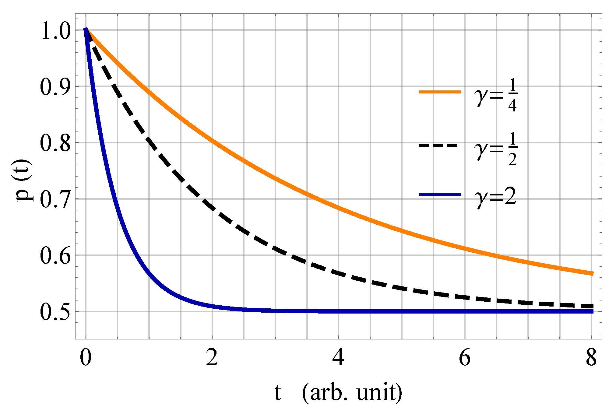
To observe in detail the properties of $p\left(t\right)$, we present three plots in Figure 1, which correspond to different values of $\theta$. One can observe how the distinguishability between two orthogonal states degenerates as the evolution continues. This phenomenon implies that the error probability in quantum communication increases due to the overlap between the basis states. One can notice that

$$\forall \gamma >0\underset{t\to \infty }{lim}p\left(t\right)=\frac{1}{2}(1+|cos\theta \left|\right),$$

(18)

which is demonstrated in Figure 1 by the fact that each plot converges to a specific value as we increase t. In particular, for $\theta =\pi /2$, we see that ${lim}_{t\to \infty }p\left(t\right)=1/2$, which proves that the states from the equator of the Bloch ball are the least efficient in information encoding if the system undergoes a majorization monotone dynamics according to (16).

7.2. Example 2: Time-Dependent Bit Flip Channel

The second example involves a time-dependent bit flip channel defined by the Kraus operators [35]

$$K_0\left(t\right)=\sqrt{\frac{1+\kappa \left(t\right)}{2}}{\mathbb{I}}_2,K_1\left(t\right)=\sqrt{\frac{1-\kappa \left(t\right)}{2}}{\sigma }_1,$$

(19)

where $\kappa \left(t\right)$ denotes the same decoherence function as in (15) and ${\sigma }_1$ is one of the Pauli matrices. As in the previous example, the dynamical map (19) is unital, which implies that the condition for majorization monotone dynamics is satisfied. Geometrically speaking, the action of this map shrinks the Bloch ball uniformly in the $YOZ$ plane, while the states on the x axis are left untouched.

For an arbitrary pair of orthogonal states, $|\psi \rangle$ and $|{\psi }_{\perp }\rangle$, we compute

$$\begin{array}{cc}\hfill p\left(t\right)& =\frac{1}{2}\left(1+\frac{1}{2}\mathrm{tr}\parallel {\rho }_1\left(t\right)-{\rho }_2\left(t\right)\parallel \right)=\frac{1}{2}\left(1+\frac{1}{2}\mathrm{tr}\parallel {\mathsf{\Lambda }}_t\left[|\psi \rangle \langle \psi |\right]-{\mathsf{\Lambda }}_t\left[|{\psi }_{\perp }\rangle \langle {\psi }_{\perp }|\right]\parallel \right)\hfill \\ \hfill & =\frac{1}{2}\left(1+e^{-\gamma t}\sqrt{{cos}^2\theta +e^{\gamma t}{sin}^2\theta \left(cosh\gamma t+cos2\varphi sinh\gamma t\right)}\right).\hfill \end{array}$$

(20)

In this case, $p\left(t\right)$ depends on both parameters that characterize an arbitrary pure qubit. To illustrate the impact of this decoherence model on the discrimination probability, we present three plots in Figure 2.

Furthermore, one can also calculate

$$\forall \gamma >0\underset{t\to \infty }{lim}p\left(t\right)=\frac{1}{2}\left(1+|cos\varphi sin\theta |\right),$$

(21)

which shows how the equilibrium value of the discrimination probability depends on the geometry of the initial state.

From (20), one can observe that if $\theta =\pi /2$ and $\varphi =0$, then $p\left(t\right)=1$ for all $t\ge 0$. It proves that the pair of orthogonal states that lie on the x axis is optimal for information encoding

$$|\psi \rangle =\frac{1}{\sqrt{2}}\left(\begin{array}{c}1\\ 1\end{array}\right),|{\psi }_{\perp }\rangle =\frac{1}{\sqrt{2}}\left(\begin{array}{c}1\\ -1\end{array}\right),$$

which implies that the information should be encoded using diagonal and antidiagonal polarization states. In other words, the x axis is a geometric representation of the one-dimensional DFS, which comprises the states that remain unchanged subject to the considered dynamical map.

7.3. Example 3: Qubit Depolarization

As the last example, we consider qubit dynamics given by a random unitary channel defined by the operators [35,48]

$$K_0\left(t\right)=\sqrt{\frac{1+3\kappa \left(t\right)}{4}}{\mathbb{I}}_2,{\left\{K_i\left(t\right)=\sqrt{\frac{1-\kappa \left(t\right)}{4}}{\sigma }_i\right\}}_{i=1,2,3}.$$

(22)

The dynamical map defined by the operators (22) describes a depolarization process that uniformly shrinks the entire Bloch ball toward the maximally mixed state. For an arbitrary pair of orthogonal states, we get the discrimination probability

$$\begin{array}{cc}\hfill p\left(t\right)& =\frac{1}{2}\left(1+\frac{1}{2}\mathrm{tr}\parallel {\rho }_1\left(t\right)-{\rho }_2\left(t\right)\parallel \right)=\frac{1}{2}\left(1+\frac{1}{2}\mathrm{tr}\parallel {\mathsf{\Lambda }}_t\left[|\psi \rangle \langle \psi |\right]-{\mathsf{\Lambda }}_t\left[|{\psi }_{\perp }\rangle \langle {\psi }_{\perp }|\right]\parallel \right)\hfill \\ \hfill & =\frac{1}{2}\left(1+e^{-\gamma t}\right).\hfill \end{array}$$

(23)

The result (23) does not depend on the parameters $\theta$ and $\varphi$ that characterize the state $|\psi \rangle$, which is consistent with the fact that this evolution is spherically symmetric. Moreover, let us consider the plots of $p\left(t\right)$ for different depolarization parameters $\gamma$. In Figure 3, one finds three plots that demonstrate the exponential decay of the distinguishability for three values of $\gamma$.

Finally, for depolarization, we see that

$$\forall \gamma >0\underset{t\to \infty }{lim}p\left(t\right)=\frac{1}{2},$$

(24)

which confirms that, in this case, there is no optimal strategy for the choice of a basis for quantum communication. The only quantum state that remains invariant under the depolarizing dynamical map is the maximally mixed state, i.e., ${\mathsf{\Lambda }}_t\left[{\rho }_0\right]={\rho }_0$ (where ${\rho }_0=1/2{\mathbb{I}}_2$), which results from the definition of majorization monotone dynamics. However, no information can be encoded on such a quantum state.

8. Conclusions

Quantum communication requires well-characterized quantum states that can be used as carriers of information. Besides protocols that guarantee the security of communication, we need to investigate external factors that can affect the entire process. A realistic framework for optical QKD should take into account different sources of errors, such as optical losses, fiber attenuation, polarization misalignment, or limited capability of single-photon detectors [52]. The same goes for quantum computers, where any feasibility study should involve distortionary phenomena, such as decoherence, off-resonance qubit evolution, and undesired qubit–qubit residual interaction in the case of nuclear magnetic resonance quantum hardware [53].

In this paper, we analyzed how the orthogonality of basis states was influenced by majorization monotone dynamics. The mathematical formalism allowed us to investigate the time evolution of an arbitrary pair of orthogonal states. The discrimination probability could be used to quantify the accuracy of the quantum communication in the time domain. For some dynamical maps, it was possible to determine optimal pairs of orthogonal states that belonged to the decoherence-free subspace. For such states, quantum information was protected from the detrimental impact of decoherence.

In each example of majorization monotone dynamics, we obtained a specific formula for the discrimination probability for an arbitrary pair of initially orthogonal quantum states. The results depended on the decoherence rate and the parameters that characterized initial qubits. Therefore, one could investigate the relation between the impact of decoherence and the geometry of input states. States from different regions of the Bloch sphere could be compared in terms of their resilience to the quantum noise caused by majorization monotone dynamics.

Further development of quantum materials is essential to explore novel methods and protocols for optical quantum communication. For example, G-centers in silicon are near-infrared photon emitters with emerging applications as single-photon sources [54]. Moreover, different frameworks that aim to protect photonic qubits from environmental noise are expected to gain relevance in future implementations [55].

Furthermore, in the future, we can consider purification procedures to reverse the detrimental impact of majorization monotone dynamics on quantum communication. In particular, quantum distillation can be implemented to regain the coherence of states contaminated by noise [56]. In addition, by introducing a second environment, either natural or engineered, we can purify a quantum state up to a certain (possibly arbitrarily small) threshold [57]. Such frameworks are intrinsically limited by bounds that result from the fundamental laws of quantum physics [58].

References

- Hayashi, M. Quantum Information: An Introduction, 1st ed.; Springer: Berlin/Heidelberg, Germany, 2006. [Google Scholar]
- Kimble, H. The quantum internet. Nature 2008, 453, 1023–1030. [Google Scholar] [CrossRef]
- Flamini, F.; Spagnolo, N.; Sciarrino, F. Photonic quantum information processing: A review. Rep. Prog. Phys. 2019, 82, 016001. [Google Scholar] [CrossRef] [Green Version]
- Walther, P.; Resch, K.J.; Rudolph, T.; Schenck, E.; Weinfurter, H.; Vedral, V.; Aspelmeyer, M.; Zeilinger, A. Experimental one-way quantum computing. Nature 2005, 434, 169–176. [Google Scholar] [CrossRef] [Green Version]
- Kok, P.; Munro, W.J.; Nemoto, K.; Ralph, T.C.; Dowling, J.P.; Milburn, G.J. Linear optical quantum computing with photonic qubits. Rev. Mod. Phys. 2007, 79, 135–174. [Google Scholar] [CrossRef] [Green Version]
- O’Brien, J.L.; Furusawa, A.; Vuckovic, J. Photonic quantum technologies. Nat. Photon. 2009, 3, 687–695. [Google Scholar] [CrossRef] [Green Version]
- Pirandola, S.; Andersen, U.L.; Banchi, L.; Berta, M.; Bunandar, D.; Colbeck, R.; Englund, D.; Gehring, T.; Lupo, C.; Ottaviani, C.; et al. Advances in Quantum Cryptography. Adv. Opt. Photon. 2020, 12, 1012. [Google Scholar] [CrossRef] [Green Version]
- Wang, H.-W.; Tsai, C.-W.; Lin, J.; Huang, Y.-Y.; Yang, C.-W. Efficient and Secure Measure-Resend Authenticated Semi-Quantum Key Distribution Protocol against Reflecting Attack. Mathematics 2022, 10, 1241. [Google Scholar] [CrossRef]
- Abushgra, A.A. Variations of QKD Protocols Based on Conventional System Measurements: A Literature Review. Cryptography 2022, 6, 12. [Google Scholar] [CrossRef]
- Schlosshauer, M. Decoherence and the Quantum-to-Classical Transition, 1st ed.; Springer: Berlin/Heidelberg, Germany, 2007. [Google Scholar]
- Alicki, R.; Lendi, K. Quantum Dynamical Semigroups and Applications; Springer: Berlin/Heidelberg, Germany, 2007. [Google Scholar]
- Rivas, Á.; Huelga, S.F. Open Quantum Systems. An Introduction; Springer: Berlin/Heidelberg, Germany, 2012. [Google Scholar]
- Yuan, H. Reachable set of open quantum dynamics for a single spin in Markovian environment. Automatica 2013, 49, 955–959. [Google Scholar] [CrossRef]
- Cai, X.; Meng, R.; Zhang, Y.; Wang, L. Geometry of quantum evolution in a nonequilibrium environment. Europhys. Lett. 2019, 125, 30007. [Google Scholar] [CrossRef]
- Manzano, D. A short introduction to the Lindblad master equation. AIP Adv. 2020, 10, 025106. [Google Scholar] [CrossRef]
- Pourkarimi, M.R.; Haseli, S.; Haddadi, S.; Hadipour, M. Scrutinizing entropic uncertainty and quantum discord in an open system under quantum critical environment. Laser Phys. Lett. 2022, 19, 065201. [Google Scholar] [CrossRef]
- Wang, Z.-M.; Ren, F.-H.; Luo, D.-W.; Yan, Z.-Y.; Wu, L.-A. Almost-exact state transfer by leakage-elimination-operator control in a non-Markovian environment. Phys. Rev. A 2020, 102, 042406. [Google Scholar] [CrossRef]
- Kyaw, T.H.; Bastidas, V.M.; Tangpanitanon, J.; Romero, G.; Kwek, L.-C. Dynamical quantum phase transitions and non-Markovian dynamics. Phys. Rev. A 2020, 101, 012111. [Google Scholar] [CrossRef] [Green Version]
- Chen, M.; Chen, H.; Han, T.; Cai, X. Disentanglement Dynamics in Nonequilibrium Environments. Entropy 2022, 24, 1330. [Google Scholar] [CrossRef]
- Dolatkhah, H.; Haddadi, S.; Hu, M.L.; Pourkarimi, M.R. Characterizing tripartite entropic uncertainty under random telegraph noise. Quantum Inf. Process. 2022, 21, 356. [Google Scholar] [CrossRef]
- Yuan, H. Characterization of Majorization Monotone Quantum Dynamics. IEEE Trans. Automat. Contr. 2010, 55, 955–959. [Google Scholar] [CrossRef]
- Bin-Mohsin, B.; Javed, M.Z.; Awan, M.U.; Budak, H.; Kara, H.; Noor, M.A. Quantum Integral Inequalities in the Setting of Majorization Theory and Applications. Symmetry 2022, 14, 1925. [Google Scholar] [CrossRef]
- Zurek, H.B. Decoherence, einselection, and the quantum origins of the classical. Rev. Mod. Phys. 2003, 75, 715–775. [Google Scholar] [CrossRef] [Green Version]
- Horodecki, R. Quantum Information. Acta Phys. Pol. A 2021, 139, 197–218. [Google Scholar] [CrossRef]
- Lidar, D.A.; Chuang, I.L.; Whaley, K.B. Decoherence-Free Subspaces for Quantum Computation. Phys. Rev. Lett. 1998, 81, 2594–2597. [Google Scholar] [CrossRef] [Green Version]
- Beige, A.; Braun, D.; Tregenna, B.; Knight, P.L. Quantum Computing Using Dissipation to Remain in a Decoherence-Free Subspace. Phys. Rev. Lett. 2000, 85, 1762–1765. [Google Scholar] [CrossRef] [Green Version]
- Bhatia, R. Matrix Analysis, 1st ed.; Springer: Berlin/Heidelberg, Germany, 1997. [Google Scholar]
- Marshall, A.W.; Olkin, I.; Arnold, B.C. Inequalities: Theory of Majorization and Its Applications, 2nd ed.; Springer: New York, NY, USA, 2011. [Google Scholar]
- von Neumann, J. Mathematical Foundations of Quantum Mechanics; Princeton University Press: Princeton, NJ, USA, 1955. [Google Scholar]
- Blum, K. Density Matrix Theory and Applications, 3rd ed.; Springer: Berlin/Heidelberg, Germany, 2012. [Google Scholar]
- von Neumann, J. Wahrscheinlichkeitstheoretischer Aufbau der Quantenmechanik. Gött. Nach. 1927, 1, 245–272. [Google Scholar]
- Landau, L. Das Dampfungsproblem in der Wellenmechanik. Z. Phys. 1927, 45, 430–441. [Google Scholar] [CrossRef]
- Shannon, C. A Mathematical Theory of Communication. Bell Syst. Tech. J. 1948, 27, 379–423. [Google Scholar] [CrossRef] [Green Version]
- Uhlmann, A. Sätze über Dichtematrizen. Math.-Naturwiss. Reihe 1971, 20, 633–637. [Google Scholar]
- Nielsen, M.A.; Chuang, I.L. Quantum Computation and Quantum Information; Cambridge University Press: Cambridge, UK, 2000. [Google Scholar]
- Kraus, K. Operations and effects in the Hilbert space formulation of quantum mechanics. In Foundations of Quantum Mechanics and Ordered Linear Spaces; Hartkämper, A., Neumann, H., Eds.; Springer: Berlin/Heidelberg, Germany, 1974; pp. 206–229. [Google Scholar]
- Kraus, K. States, Effects and Operations, Fundamental Notions of Quantum Theory; Springer: Berlin/Heidelberg, Germany, 1983. [Google Scholar]
- Audenaert, K.M.R.; Scheel, S. On random unitary channels. New J. Phys. 2008, 10, 023011. [Google Scholar] [CrossRef]
- Helm, J.; Strunz, W.T. Quantum decoherence of two qubits. Phys. Rev. A 2009, 80, 042108. [Google Scholar] [CrossRef] [Green Version]
- Bengtsson, I.; Życzkowski, K. Geometry of Quantum States: An Introduction to Quantum Entanglement, 2nd ed.; Cambridge University Press: Cambridge, UK, 2017. [Google Scholar]
- Helstrom, C.W. Quantum detection and estimation theory. J. Stat. Phys. 1969, 1, 231–252. [Google Scholar] [CrossRef] [Green Version]
- Holevo, A.S. Statistical decision theory for quantum systems. J. Multivar. Anal. 1973, 3, 337–394. [Google Scholar] [CrossRef] [Green Version]
- Fuchs, C.A.; van de Graaf, J. Cryptographic distinguishability measures for quantum-mechanical states. IEEE Trans. Inf. Theory 1999, 45, 1216–1227. [Google Scholar] [CrossRef] [Green Version]
- Bennett, C.H.; Brassard, G. Quantum Cryptography: Public key distribution and coin tossing. In Proceedings of the IEEE International Conference on Computers, Systems and Signal Processing, Bangalore, India, 9–12 December 1984; pp. 175–179. [Google Scholar]
- Ekert, A.K. Quantum cryptography based on Bell’s theorem. Phys. Rev. Lett. 1991, 67, 661–663. [Google Scholar] [CrossRef]
- Lidar, D.A.; Brun, T.A. (Eds.) Quantum Error Correction; Cambridge University Press: New York, NY, USA, 2013. [Google Scholar]
- Wu, Y.; Lee, Y. Self-Orthogonal Codes Constructed from Posets and Their Applications in Quantum Communication. Mathematics 2020, 8, 1495. [Google Scholar] [CrossRef]
- Czerwinski, A. Applications of the Stroboscopic Tomography to Selected 2-Level Decoherence Models. Int. J. Theor. Phys. 2016, 55, 658–668. [Google Scholar] [CrossRef] [Green Version]
- Palma, G.M.; Suominen, K.A.; Ekert, A.K. Quantum computers and dissipation. Proc. R. Soc. Lond. Ser. A 1996, 452, 567–584. [Google Scholar]
- Bardhan, B.R.; Anisimov, P.M.; Gupta, M.K.; Brown, K.L.; Jones, N.C.; Lee, H.; Dowling, J.P. Dynamical decoupling in optical fibers: Preserving polarization qubits from birefringent dephasing. Phys. Rev. A 2012, 85, 022340. [Google Scholar] [CrossRef] [Green Version]
- Liu, Z.D.; Lyyra, H.; Sun, Y.N.; Liu, B.-H.; Li, C.-F.; Guo, G.-C.; Maniscalco, S.; Piilo, J. Experimental implementation of fully controlled dephasing dynamics and synthetic spectral densities. Nat. Commun. 2018, 9, 3453. [Google Scholar] [CrossRef] [PubMed] [Green Version]
- Caputo, C.; Simoni, M.; Cirillo, G.A.; Turvani, G.; Maurizio, Z. A simulator of optical coherent-state evolution in quantum key distribution systems. Opt. Quant. Electron. 2022, 54, 689. [Google Scholar] [CrossRef]
- Simoni, M.; Cirillo, G.A.; Turvani, G.; Graziano, M.; Zamboni, M. Towards compact modeling of noisy quantum computers: A molecular-spin-qubit case of study. J. Emerg. Technol. Comput. Syst. 2022, 18, 1550–4832. [Google Scholar] [CrossRef]
- Schenkel, T.; Redjem, W.; Persaud, A.; Liu, W.; Seidl, P.A.; Amsellem, A.J.; Kanté, B.; Ji, Q. Exploration of Defect Dynamics and Color Center Qubit Synthesis with Pulsed Ion Beams. Quantum Beam Sci. 2022, 6, 13. [Google Scholar] [CrossRef]
- Damodarakurup, S.; Lucamarini, M.; Di Giuseppe, G.; Vitali, D.; Tombesi, P. Experimental Inhibition of Decoherence on Flying Qubits via “Bang-Bang” Control. Phys. Rev. Lett. 2009, 103, 040502. [Google Scholar] [CrossRef] [PubMed] [Green Version]
- Fang, K.; Wang, X.; Lami, L.; Regula, B.; Adesso, G. Probabilistic Distillation of Quantum Coherence. Phys. Rev. Lett. 2018, 121, 070404. [Google Scholar] [CrossRef] [Green Version]
- Ticozzi, F.; Viola, L. Quantum resources for purification and cooling: Fundamental limits and opportunities. Sci. Rep. 2014, 4, 5192. [Google Scholar] [CrossRef] [PubMed]
- Fang, K.; Liu, Z.W. No-Go Theorems for Quantum Resource Purification. Phys. Rev. Lett. 2000, 125, 060405. [Google Scholar] [CrossRef] [PubMed]
Figure 1.
Plots of according to (17) for three values of . Other parameters: (arb. unit).
Figure 2.
Plots of according to (20) for three combinations of and . Other parameters: (arb. unit).
Figure 3.
Plots of according to (23) for three values of .
Publisher’s Note: MDPI stays neutral with regard to jurisdictional claims in published maps and institutional affiliations. |
© 2022 by the author. Licensee MDPI, Basel, Switzerland. This article is an open access article distributed under the terms and conditions of the Creative Commons Attribution (CC BY) license (https://creativecommons.org/licenses/by/4.0/).
Share and Cite
MDPI and ACS Style
Czerwinski, A. Quantum Communication with Polarization-Encoded Qubits under Majorization Monotone Dynamics. Mathematics 2022, 10, 3932. https://0-doi-org.brum.beds.ac.uk/10.3390/math10213932
AMA Style
Czerwinski A. Quantum Communication with Polarization-Encoded Qubits under Majorization Monotone Dynamics. Mathematics. 2022; 10(21):3932. https://0-doi-org.brum.beds.ac.uk/10.3390/math10213932
Chicago/Turabian StyleCzerwinski, Artur. 2022. "Quantum Communication with Polarization-Encoded Qubits under Majorization Monotone Dynamics" Mathematics 10, no. 21: 3932. https://0-doi-org.brum.beds.ac.uk/10.3390/math10213932
Note that from the first issue of 2016, this journal uses article numbers instead of page numbers. See further details here.