
A Novel Optical-Based Methodology for Improving Nonlinear Fourier Transform
by
 , , , and
Julian Hoxha
1,*,
Wael Hosny Fouad Aly
1 ,
,
Erdjana Dida
2,
Iva Kertusha
1 and
Mouhammad AlAkkoumi
1 1
College of Engineering and Technology, American University of the Middle East, Egaila 54200, Kuwait
2
Engineering and Technology, American College of the Middle East, Egaila 54200, Kuwait
*
Author to whom correspondence should be addressed.
Mathematics 2022, 10(23), 4513; https://0-doi-org.brum.beds.ac.uk/10.3390/math10234513
Submission received: 23 October 2022
/
Revised: 18 November 2022
/
Accepted: 25 November 2022
/
Published: 29 November 2022
(This article belongs to the Special Issue Novel Mathematical Methods in Signal Processing and Its Applications)
Abstract
:The increasing demand for bandwidth and long-haul transmission has led to new methods of signal processing and transmission in optical fiber communication systems. The nonlinear Fourier transform is one of the most recent methods proposed, and is able to represent an integrable nonlinear Schrödinger equation (NLSE) channel in terms of its continuous and discrete spectrum, to overcome the limitation of the bandwidth imposed by the Kerr effect on silica fibers. In this paper, we will propose and investigate the Boffetta-Osburne method for the direct nonlinear Fourier implementation, and the Gel’fand-Levitan-Marchenko equation for the inverse nonlinear Fourier, as only the continuous part of the nonlinear spectrum will be used to encode information. A novel methodology is proposed to improve their numerical implementation with respect to the NLSE, and we analyze in detail how the improved algorithm can be used in a real optical system, by investigating three different modulation schemes. We report increased performance transmission and consistency in the numerical results when the proposed methodology is applied. Our results show that b-modulation will increase the Q-factor by 2 dB with respect to the other two modulations. The improvement results with our proposed methodology suggest that b-modulation applied only to a continuous part of the nonlinear spectrum is a very effective method for maximizing both the transmission bandwidth and distance in optical fiber communication systems.
Keywords:
nonlinear Fourier transform; numerical algorithms; nonlinear Schrödinger equation; modulationMSC:
34L25; 35Q60; 35Q55; 35Q94; 65J10; 76B15; 78A46; 94A14; 94A131. Introduction
The global data traffic is exponentially increasing due to large bandwidth requests coming from different services, such as high-definition interactive video, high-resolution editing video, and distributed systems [1]. The global internet bandwidth has increased by 28% in 2022, reaching approximately 1 Pbps [2]. Optical fiber is one of the most widely used transmission mediums when compared to other backbone networks. As opposed to various communication channels, optical fiber communication systems cannot be modeled as a linear channel under Gaussian perturbations, since the transmission in this medium is indeed nonlinear and mainly affected by three physical effects: (1) Kerr nonlinearity, (2) additive white Gaussian noise, and (3) chromatic dispersion. These effects are considered as undesirable, and digital signal processing is used to mitigate them at the receiver side [3,4].
Nowadays, a completely different approach is applied where nonlinearity is treated as a property of nonlinear channels. This can help to develop new transmission techniques. Nonlinear Fourier Transform (NFT) is one of the most recent methods studied for transmitting information in optical fiber communication systems in order to overpass the current state-of-the-art of multi-user transmission in wavelength division multiplexing (WDM) systems. From a mathematical point of view, the NFT is able to represent an integrable nonlinear dispersive partial differential equation (PDE) in terms of its continuous and discrete spectrum [5]. As the wave propagates over the channel under different nonlinear effects, the impact of the channel on its spectral components will be simply given by independent linear equations, as will be shown later. This technique is very effective in multi-user channels where the information can be encoded on the nonlinear part of the spectrum. This results in reduced inter-channel interference, improved signal to noise ratio, and better spectral efficiency [6,7,8,9]. On the other hand, the implementation of this technique requires physical changes in the current deployed infrastructure [10].
The NLSE is most widely solved using the numerical method, and hence, a larger number of numerical solutions have been proposed for it. The main reason behind the ability for the NLSE ability to be resolved numerically is that it does not have direct solutions known in analytical form, except for some specific cases. Taha et al. [5,11] made a comparative analysis of the numerical methods and the finite difference schemes used to solve the problem associated with NLSE. The analysis included the Ablowitz-Ladik scheme developed using notions related to the Inverse Scattering Transform (IST), nowadays called NFT in the telecommunications system community.
The logic behind NFT is quite simple. If the information signal would have to propagate through a highly nonlinear optical fiber governed by the NLSE equation, then its waveform at a desired distance could be associated with a linear operator that we need to find. This linear operator is an infinite dimensional matrix with a spectrum that consists of continuous and discrete eigenvalues. It turns out that these eigenvalues are invariant of the NLSE during the propagation through the fiber. The goal is to find a modulation scheme where we can modulate these eigenvalues, thus overcoming the nonlinear effect limitation. The first idea based on this simplified observation was published around 30 years ago, where eigenvalue communication was proposed to substitute for the on–off key solution for transmission in optical fiber communication systems [12]. The same idea was re-proposed and experimentally verified later in [13,14,15]. However, many researchers observed that there is no need to have an unchanged shape in the optical pulse in the NFT domain, as the channel effect will be a linear one. Moreover, this effect can be easily equalized at the receiver side, or pre-compensated at the transmitter side.
Several published papers exploit different degrees of freedom of the NFT and the Inverse NFT (INFT), using both discrete and continuous eigenvalues from the nonlinear spectrum. This results in a data transmission over the optical fiber similar to orthogonal frequency division multiplexing (OFDM) [16,17]. Hence, multiple users can access the optical channel.
Other researchers focused only on the discrete part of the spectrum and proved experimentally the reliability of the NFT and INFT [18,19,20,21,22,23,24]. The sole usage of the continuous part was studied in several papers [25,26,27,28,29]. Compared to using only the discrete part, this method resulted in increased performance in terms of spectral efficiency, transmission over long distances, and lower complexity at the receiver side. Dual polarization experimental transmission based on NFT was also reported in [30,31]. Full spectrum modulation using both continuous and discrete nonlinear parts of the spectrum was reported in [32], but this was limited only to back-to-back transmission.
Several numerical algorithms are proposed in the literature to solve the direct NFT and INFT [33]. To compute the direct NFT, we can generalize the algorithms into two main methods: (1) the Ablowitz-Ladik method [34,35] and (2) the Boffetta-Osborne Method [36]. To compute the INFT, we can generalize the algorithms into two main methods: the Darboux transformation method [37] and the Gelfand-Levitan-Marchenko (GLM) method [38]. Fast non linear Fourier transform (FNFT) is also analyzed in several papers, and is published online as a tool to reduce the implementation complexity of the NFT [39,40]. The purpose of FNFT is to develop an algorithm that computes a fast product between polynomials that are used to find the continuous spectrum. The NFT and INFT are relatively new methods, where the associated numerical implementations have not yet been fully addressed, especially its application in the field of optical fiber telecommunications.
Analytical solutions of the NLS have also been recently proposed, in [41,42,43,44,45]. Unfortunately, they cannot be directly applied for optical communication, and numerical solutions with lower complexity are still the only alternative to solve NLS.
In this paper, we propose a methodology to improve both the direct NFT and INFT numerical implementations in order to obtain only the continuous part of the nonlinear spectrum. The reason behind choosing this approach as a preliminary results shows a potential deployment in the future of the optical fiber transmission, reported in [9]. Compared to existing wavelength division multiplexing (WDM) systems, the continuous spectrum has a higher spectral efficiency and reduced complexity at the receiver side.
For the direct NFT numerical implementation, we will investigate in detail the Boffetta-Osborne method, as it cannot be simplified using polynomials, in order to make use of the fast NFT (FNFT), as in [46,47]. An explanation on how this method is improved for NFT, and how it will affect the INFT implementation without performance degradation, will be given below.
For the INFT numerical implementation, we will solve and investigate numerically the GLM integral equations. These equations can represent a complexity that is comparable to FNFT. We have identified the parameters’ values for maximizing the performance, and have used them to compare three different types of modulations that are proposed recently.
In the main strength of our work, we present the complex mathematical tools that are involved in a simplified form, and minimize errors coming from multiple numerical approximations. Being accessible to the NFT research community, this work will help to simulate the optical fiber communication system with high accuracy, avoiding expensive and time consuming experimental setups in laboratories. Compared to the FNFT, the algorithm has higher complexity, but if carefully designed, it can give better performance.
The rest of the paper is organized as follows: in Section 2, we analyze in detail the direct NFT, and explain the numerical procedure to recover the continuous scattering coefficient. In Section 3, we analyze the procedures to be followed, starting from the INFT theory until an accurate numerical simulation of Marchenko system is reached. In Section 4, we validate our numerical algorithms, and in Section 5, we compare the performance of three different types of modulations proposed in the literature. The conclusion is given in the last section.
2. Scattering Coefficient for Nonlinear Fourier Transform
The evolution of the slowly varying complex-valued envelope of the scalar electric field propagating in a single mode optical fiber, neglecting the effects of polarization and attenuation, but taking into account the chromatic dispersion and nonlinear refraction (Kerr effect), is the following:
where z is the space coordinate, t is the time reference frame co-moving with the group velocity of the signal envelope, chromatic dispersion, and nonlinear parameter. In particular, represents the dispersion of the group velocity, which causes an enlargement of the impulse during propagation; parameter models the nonlinear refraction, which is the dependence of the refractive index on the optical field intensity.
To simplify Equation (1), we will first multiply it by the imaginary number i, and then we will make the following substitution: , , , with in power units, where is a free normalization parameter in units of time, , a constant number that represents the nature of the signal inside the optical fiber; the following parameters are all positive quantities: , , > 0. By selecting all these parameters to have the following relation: , for example by choosing , then we will obtain a simplified form of Equation (1) as the following:
when , then the solution envelope of Equation (2) will be solitons. These are usually called deep water waves. In the case of , then the soliton cannot exist and the solution is called shallow water as it is similar to the Korteweg-de Vries (KdV) equation. In this work, we are interested in a deep water waves solution with .
Next, we will explain how the NFT method works. Let us suppose that we have a differential equation that describes the behavior of in (2), and we want to solve it using NFT. First, we have to find two linear operators and A that are dependent on (and possibly the derivatives of ) that will describe a scattering problem of the following system:
where is the eigenvalue, w is the eigenfunction, and the subscript denotes the derivative.
The operators and A will have to be chosen according to a certain criteria as explained below: we look for an adequate evolutionary equation over the spatial dimension for w, assuming that the Schwarz Theorem applies; that is, . We are going to take the derivative of the first equation in (3) with respect to space, supposing that: . After some simple manipulation, we can find the following relation: . If we want this to be valid for every w, then we have to impose the following Lax equation [48]:
This equation contains a condition of compatibility for the operators, which in this case are called Lax pairs and can be possibly solved using the PDE for u. To use the NFT, we need to associate Equation (2) with some Lax pairs. Suppose we have the following Lax pairs [49]:
The first differential operator in (5) gives us the associated eigenvalue problem to the NLSE, while the second one is the temporal evolution of the eigenfunction, as explained in the following theorem.
Theorem 1.
Proof of Theorem 1.
We first apply the operator A to as
and after this, we apply to obtain two components: and . We perform the same thing, but this time we first apply and then A to obtain the first component . Finally, we can find: and , which is the NLSE in Equation (2). □
After choosing the Lax pair, we need to analyze the direct NFT associated with the following equation:
For the NFT method to work, we need to impose that at infinity, our solution u will decay to zero, for . Equation (8) will be approximated with the following result: with and , whose solutions are simple to calculate.
To form the basis of the solutions space of Equation (8), we can choose from the following Jost functions, defined as limit [48]:
The overbar sign means that two autofunctions are in straight relation with each other. For example, the existence of will imply also that of , given that if the first function is a solution to , then the second will also be a solution that is linearly independent from the first one:
Proposition 1.
The four solutions ϕ, , φ, are independent in pairs.
Proof of Proposition 1.
The Wronskian of two autofunctions can be easily found to be 1 as: . □
The equation should have only two linear independent solutions, and so and should be linearly dependent with respect to the pair and , as follows:
This is true when , as the four functions are limited, and in that case, these equations will define the relative four scattering coefficients data denoted by , , , . We note here that these scattering coefficients are time invariant, a property that will be used for transmitting data over the optical fiber.
To find the spatial evolution of the scattering data, under the hypothesis that: holds for every z, the operator A is such that:
which is the matrix representation that we will use to find the spatial evolution of the scattering data. The new Jost functions will be defined now as:
They are valid for every z, they will solve equation Equation (8), and they will satisfy both Equations (9) and (10).
Let’s take the spatial derivative of Equation (12) with the new Jost function, and after some manipulation, we obtain the following relations:
We can write the spatial evolution of the continuous scattering data, starting from the initial ones as follows:
When the condition is true, then we can define the discrete spectrum of the Lax operator, which consists of a finite number of discrete eigenvalues. The discrete scattering coefficient corresponding to these discrete eigenvalues can be computed by using Equations (12) and (13). In this work, we will focus only on the continuous parameter and its associated continuous scattering coefficient. Altogether, they will define our nonlinear spectrum of the signal .
Numerical Method for the Continuous Scattering Coefficient
We have developed a numerical algorithm to find the continuous scattering coefficient of the Lax equation: with the initial condition signal . We followed the idea introduced in the article by Boffetta and Osborne [36].
The algorithm will use a discretization of in samples as: , where is the total width of the function u centered at , such that for and .
The steps followed to find out the numerical algorithm for the continuous scattering coefficient when are given below:
Step 1. We need to solve numerically the Lax equation: , and find an equation that provides us with a relationship between and for .
Instead of solving it directly, we will first assume that is constant in the interval . After this, we are going to associate to it the equation, , which is equivalent to . is an approximation of with constant step. We are going to solve numerically the following Cauchy problem, in an iterative way:
with
in order to find the new starting point , having already previously found . Solving equation Equation (21) until will give us the following iteration:
where represents the effect of the operator on interval . In particular, we have that:
An explicit expression of can be calculated for our case through the definition of the exponential of a matrix:
and taking into account Taylor’s series of the cosh and sinh functions, for the matrix taken into consideration. The obtained result is:
with being a complex number. If we introduce a new vector as:
with , Equation (23) will be transformed into:
with
We take as the starting point and iterate it until we find the following relation for a generic :
having the relation:
and define S the scattering matrix as:
In Equation (31), we found a relation that connects and for . In particular, we performed it for the case when . Therefore, we can move to the second step of our algorithm, starting from this value of t.
Step 2. Assume that the conditions (9) and (10) are satisfied for , given that for . The operator (depending on will assume its asymptotic configuration as:
and so for every , the following relation should hold:
For , we can rewrite Equation (34) as:
Step 3. Given that: , we can substitute Equation (10) into it, to find the following relation for the same value of t:
Use Equations (27), (31), (35) and (36) to find an expression for . Using simple algebraic steps, we can have a numerical approximation of both the continuous scattering data and as:
A summary of the main steps involved in the calculation of continuous scattering data is presented below:
3. The Inverse Nonlinear Fourier Transform Method
In following section, we will use the scattering data found in the previous section to find its relationship with the solution of the NLSE equation. We will first give without proof the following theorem that will be an important step towards the Gel’fand-Levitan-Marchenko equation [49].
Theorem 2.
In order to obtain the Gel’fand-Levitan-Marchenko equation, we have to consider that should decay fast enough in order to extend Equation (12) to the upper part of the complex plane in such a way as to satisfy the following relation of the Jost functions and continuous data scattering:
If we substitute (39) and (40) in (43) and we also define the function , we can easily recover the Gel’fand-Levitan-Marchenko equation given as:
The important case studied in this paper is when the discrete scattering data do not exist, , and is defined as the inverse Fourier transform of . The ratio is also called the reflection coefficient or spectral amplitude of the nonlinear spectrum. Fast Fourier transform (FFT) can be used to compute it.
Making the following variable change in (44), will transform the Gel’fand-Levitan-Marchenko equation into two equations called Marchenko systems, which will highly simplify our numerical simulation. If we define: and as our two auxiliary functions, we can substitute Equation (44) equivalently with the following Marchenko system:
Equation (45) should be now solved numerically. Observe that in this way the quadrature formulas that we will use for the approximation of the two integrals that will be applied on the same interval and on the same variable. Note that to apply such quadrature formulas, it will be necessary to approximate the domain of function F, as explained in the next subsection.
3.1. Procedure for the Numerical Simulation of
The purpose of this section is to find a procedure to numerically simulate Equation (45). We need first to define the domain of . FFT will be used in this regard, together with some sampling constraints to satisfy the sampling theorem. This can be easily recognized inside the integral with some minor changes.
Let us suppose that the domain of will be in a range between with total discrete points where we have to apply FFT. We denote these discrete points as: , with and frequency resolution. In a strict relation with these points, we will have the non-zero time domain of where we will define the sampling points as: with and time resolution. The number of points for both domains and will be the same in this work. Our scope is to find the relationship between and for both the time and frequency domains.
Starting with the smallest frequency associated with the interval that will be related to as: , we also have and .
In order to solve Equation (44), we developed the following procedure:
- Approximate the values , such that if and to estimate the domain for .
- Control if .
- (a)
- If True, define first and perform the following change in the variables and :and .
- (b)
- If False, divide by 2 the step until point (a) is satisfied.
- Select the resolution in frequency based on the total number of points as:
- Select the resolution in time as:
- Find the spatial evolution of the spectral amplitude by sampling on the grid constructed for , and apply the inverse FFT in order to find the vector on the grid with amplitude:
- Select a user-defined variable called tolerance, , and check if the function is less than it at the edge only, in order to better approximate its domain. We will differentiate between two cases:
- (a)
- If , then the approximated support and the corresponding grid are chosen such that we can apply the quadrature formulas approximating the integrals to be computed in the Marchenko system of Equation (3.5).
- (b)
- Otherwise, we multiply by 2 the total number of points and restart from the second step of this numerical algorithm.
Following this procedure, we will be able to properly represent the signal and the integral of the function .
3.2. The Numerical Method Algorithm for the Marchenko System
Given the above considerations, the points on which we will decide to approximate the function will be equally spaced at a distance . The points where we will find are collected in the following vector: , where and are extreme points of this vector.
To solve the Marchenko system in Equation (45), we are going to use the Nyström method, approximating the integrals by means of a quadrature formula to derive a discrete system to be solved through an appropriate method. In particular, we want to find for . The system in (45) with will be:
Equation (49) should be solved numerically. We observe that inside the integral, we need to evaluate and for values of higher than zero. As a result, we need to solve for the values of . In particular, we are going to take and r from the same domain where is the first value of m, such that we are outside the domain of F. The reason for this choice is that such a domain should take into account the fact that we know the support of F, which is evaluated in both integrals as . The sampling step of variable r where we will integrate is: . Now, we can finally approximate both integrals in Equation (49) using the Simpson rule to find the system of equations:
where , , . The system in Equation (50) can be represented using a matrix notation such as:
where , , , are known variables. The unknown variables are:
In Equation (51), we are interested in the first component of . After finding from the first part of the system, we substitute it in the second part, and then solve the following system:
Once we have solved it, we are able to find out the signal propagated at a desired distance z:
In summary, to find out the solution of Equation (2) through the implementation of the INFT (in this case, when for every ), we need to follow the steps below:
- Based on the above algorithm, we first need to find the scattering data and , and their ratio .
- We need to find the spatial evolution of continuous spectral amplitudes by multiplying them with (step 2 should be applied only in case we will transmit the signal in an optical fiber described by Equation (2)).
- Find using IFFT, as explained above.
4. Validation of the NFT and INFT Algorithm Implementations
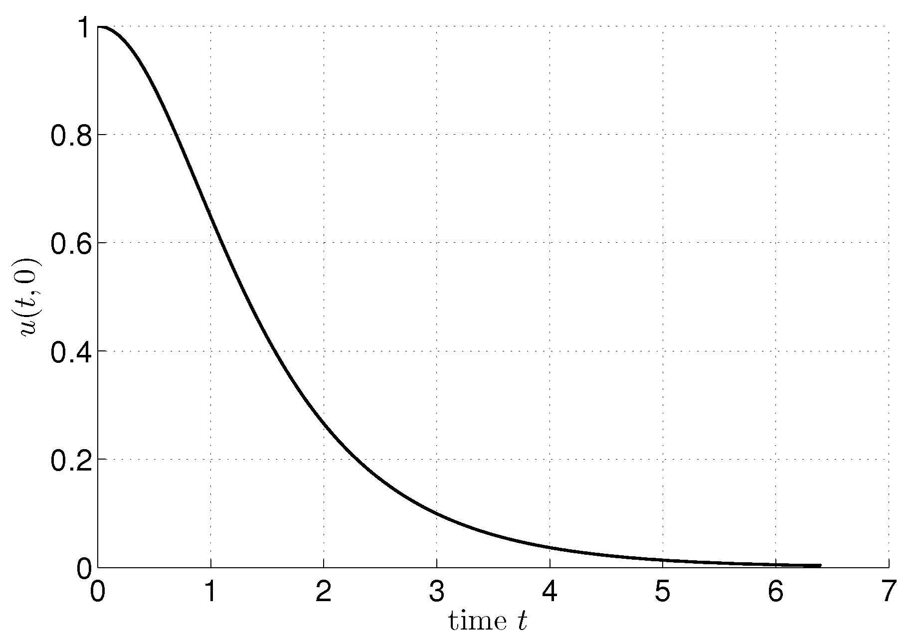
To verify our algorithm implementation for both the direct and inverse nonlinear Fourier methods, we have run multiple tests on soliton pulses taken as the initial condition with a well-known analytically closed form solution. The initial condition of our simulation is the hyperbolic secant function shown also in Figure 1:
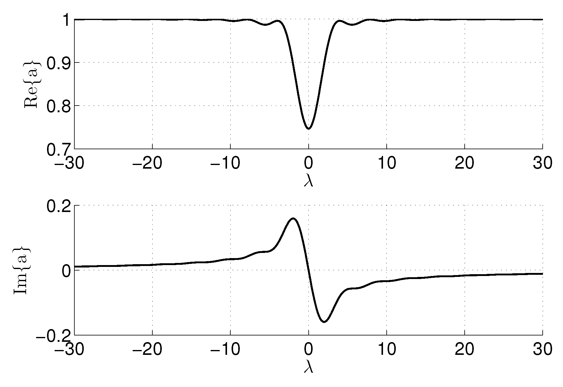
We can theoretically find the closed form solution of the scattering data, as in [50]:
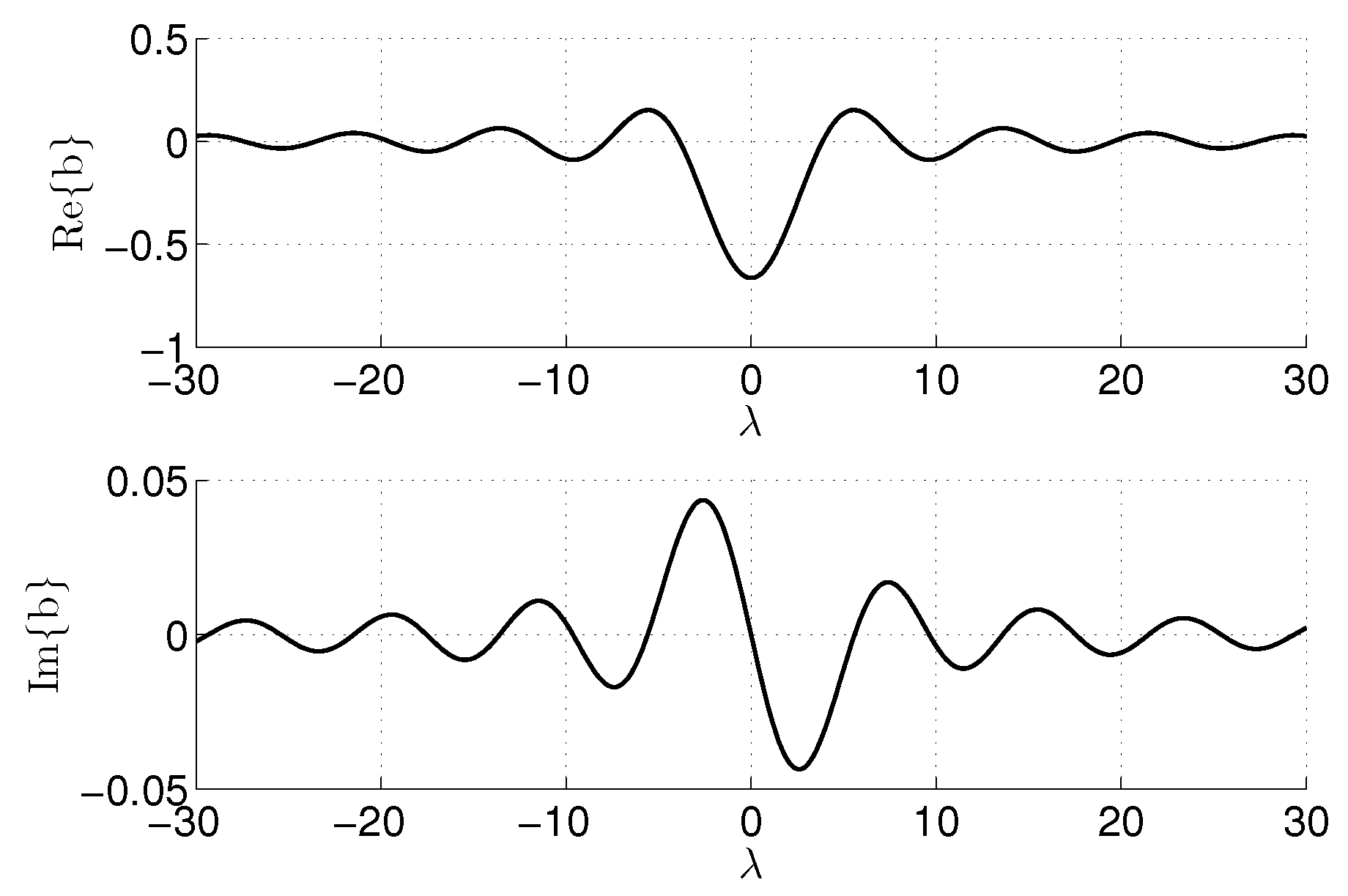
In Figure 2 and Figure 3, we show the continuous scattering data obtained from Equation (55) using the NFT algorithm described in the previous sections.
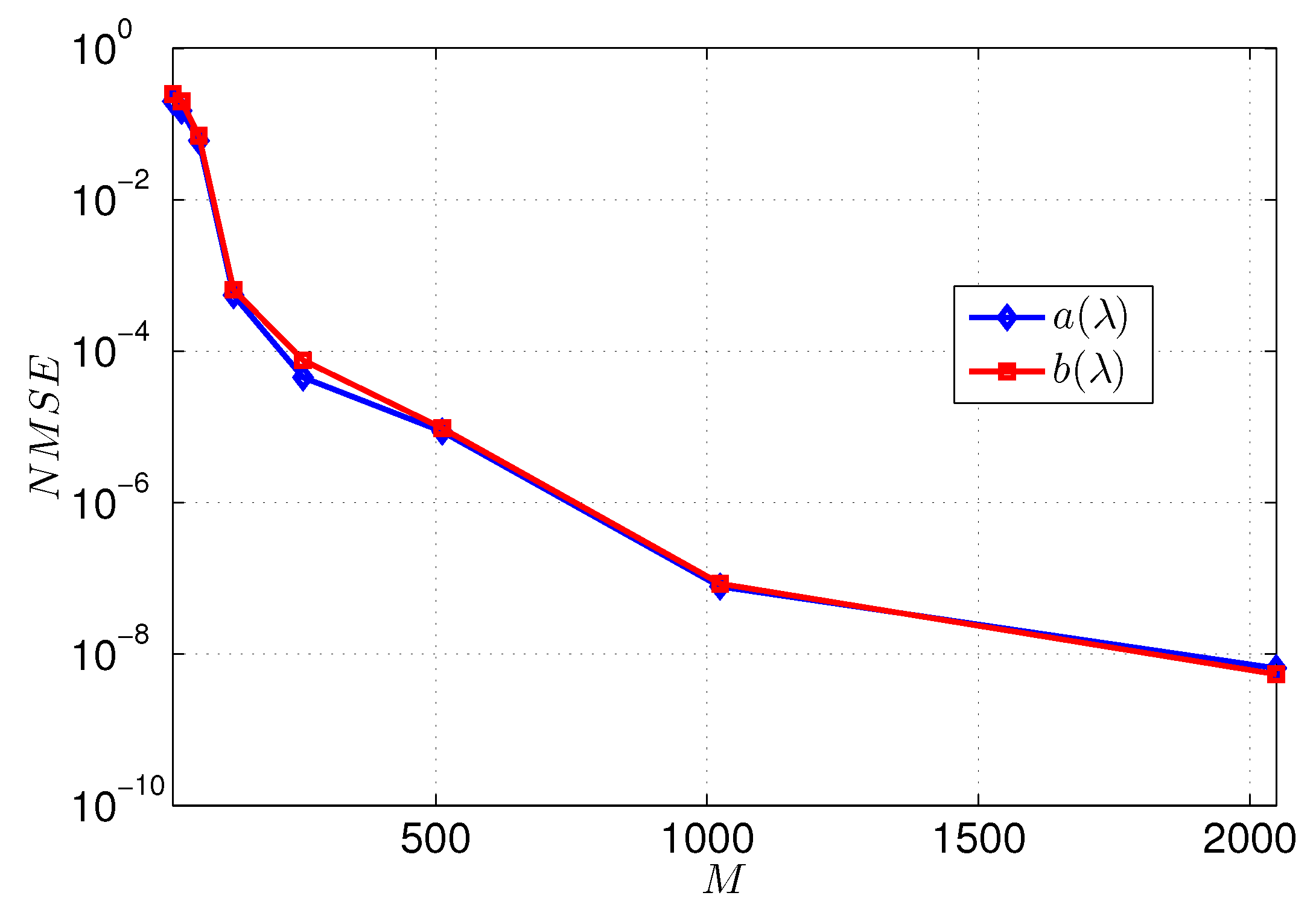
The difference between the analytical continuous scattering, , and the numerical one, , is measured in terms of the normalized means squared errors (NMSEs), defined as:
We compare the numerical results obtained with the proposed modified algorithm similiar to [36] and theoretical one given in Equations (56) and (57), for different numbers of discrete points as shown in Figure 4. We have assumed a truncated soliton pulse in the range , and a spectral parameter . The NMSE is used to measure the differences for both scattering coefficients and in order to understand how much the numerical simulations will deviate from the analytical one as a function of M. If , it means that is discretized in points. The results are highly correlated to M, as can be observed from Figure 4. If M will increase, the NMSE will also increase more and more between the numerical and theoretical results.
For further verification of our numerical algorithm procedure for the calculation of scattering data, we have checked if the following condition is satisfied (which we know that it should be always true):
For a fixed , we have obtained an error that is approximately , that is: ; consequently we can conclude that the proposed methodology has been well implemented and that it is working.
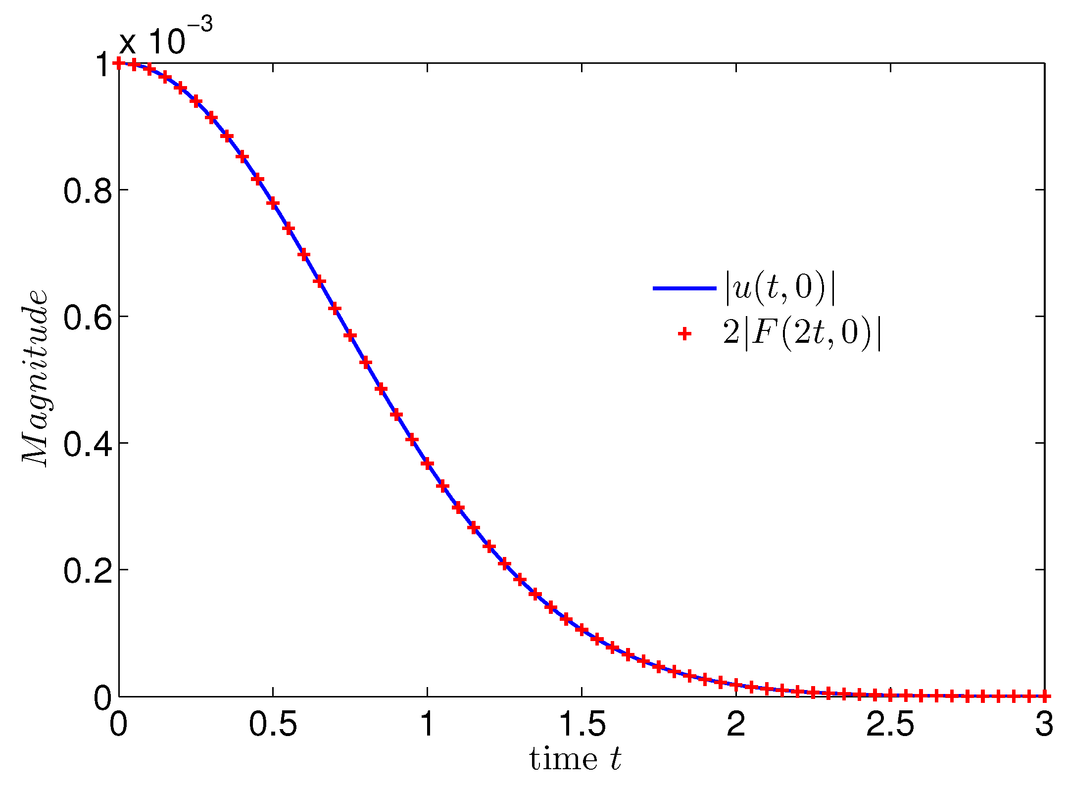
To verify for , we recall that can be found from (41) and (44), and assuming and , we have that: and . When is very small, we can assume that K and F are also small. It follows that the third addendum of Equation (44) can be negligible and we can consider: .
Assuming as an initial condition: , we can simply use the FFT to find out , taking into account strictly following the algorithm shown in the section above. The domain of is selected based on the maximum value that we have observed from the ratio of , which is in the order of , such that: . In addition, to verify the hypothesis according to which and knowing that the maximum of is , we can assume that the domain of is the interval where . We are going to look for the number of points N on which to calculate and based on the above observation.
In Figure 5, we show the result of both functions |u(t, 0)| and 2|F(2t, 0)| with N = 128, which looks very similar to each other. Selecting the right number of points N is very important, as the two functions will not look so similar to each other in the case where N is lower than 128.
5. Applications of NFT and INFT on an Optical Communication System
In this section, we will apply our proposed implementation of the NFT/INFT algorithms on a modulated signal used in optical communications. The information is encoded in continuous scattering data at the transmitter side and is decoded on the receiver side using both NFT and INFT numerical methods (as explained in the previous sections). We call this a naive implementation as it is in principle simple, but it has some disadvantages that we are going to note below. The second modulation that we will investigate is similar to the previous one, with the difference of better controlling the pulses in the time and frequency domains. Lastly, we will apply our NFT/INFT algorithm to the recently proposed method called b-modulation, where only will be used to encode the information at the transmitter side.
The nonlinear Fourier transform transmission system will exploit its orthogonality property to allow different users to transmit at the same time in optical fiber medium without any interference with each other. This is similar to the traditional OFDM that is used in almost all new wireless and wired technologies. The scenario that we are going to investigate will involve only the continuous part of the nonlinear spectrum, as the discrete part will increase the complexity at the receiver side. The use of a root searching algorithm is needed, and it is difficult to control their number. In a numerical simulation, we will make sure that there is no discrete part of the nonlinear spectrum.
The first modulation where we are going to test our implementation of NFT/INFT algorithm is originally proposed in [16]. Suppose we have the following quadrature phase shift keying (QPSK) modulated signal expressed in the time domain as:
where complex symbols, is the pulse duration, and is the root raised cosine function with unit energy and roll off factor . Let us also define: , the linear Fourier transform of our modulated signal. In the first modulation, the linear spectrum is mapped directly to the continuous nonlinear spectrum defined as the ratio between scattering data, called the reflection coefficient: . In order to compute the numerical sample in the time domain, we use the INFT algorithm as explained in the previous sections. The transmitted signal in the optical fiber will be:
At the receiver side, the NFT algorithm is used to obtain:
The channel equalization is also applied to obtain the transmitted non linear spectrum as:
The equalization is performed by inverting the effect of the channel, which is simply a phase shift in the nonlinear Fourier transform. An inverse Fourier transform followed by a match filter are used to recover the received symbols:
where is an estimation of in case the channel is affected by white Gaussian noise.
In the second modulation that we are going to investigate, the reflection coefficient is not obtained directly from mapping the linear Fourier transform, but from the following transformation to ensure that the signals have the same energy in linear and nonlinear space:
The third modulation to test our algorithm is called b-modulation. The data are encoded only on as part of the nonlinear spectrum with the following transformation:
where:
The continuous scattering data are related to as:
where denotes the Hilbert transform. The reflection coefficient will be denoted as . The details of b-modulation are already discussed in several other papers [30,51,52].
We conducted different simulation in MATLAB to transmit the three modulated signals in an optical fiber medium of total length 1600 km. The fiber was divided into 20 spans of 80 km each, where at the end of each span, white noise originating from distributed Raman amplification was added, with a noise figure of 4 dB. The optical fiber dispersion parameter is = −20.4 ps2/km, and the nonlinear coefficient is = 1.3 W km. At the receiver side, we are going to measure the performance using the Q-factor in dB found directly from the constellation affected by the white noise, as in [53]:
For historical reasons, the performance in optical systems are usually measured in terms of the quality Q-factor, given as: , where is the inverse complementary error function, and is the bit error rate. For a fixed , Q-factor is equal to 9.8 dB. Systems with a Q-factor of less than 9.8 dB will fail to work, as the number of errors is very large. We can think of this value as a lower bound for our system to work. The reason for why we are using Equation (69) as a quality parameter is because the number of transmitted symbols in our numerical simulation is only 1024, and the minimum that we can achieve is only . To fully investigate the system, even for lower , we use Equation (69). Because the oversampling factor used in this work is 40, we cannot increase the number of symbols to achieve a lower , as the computation cost will be very high.
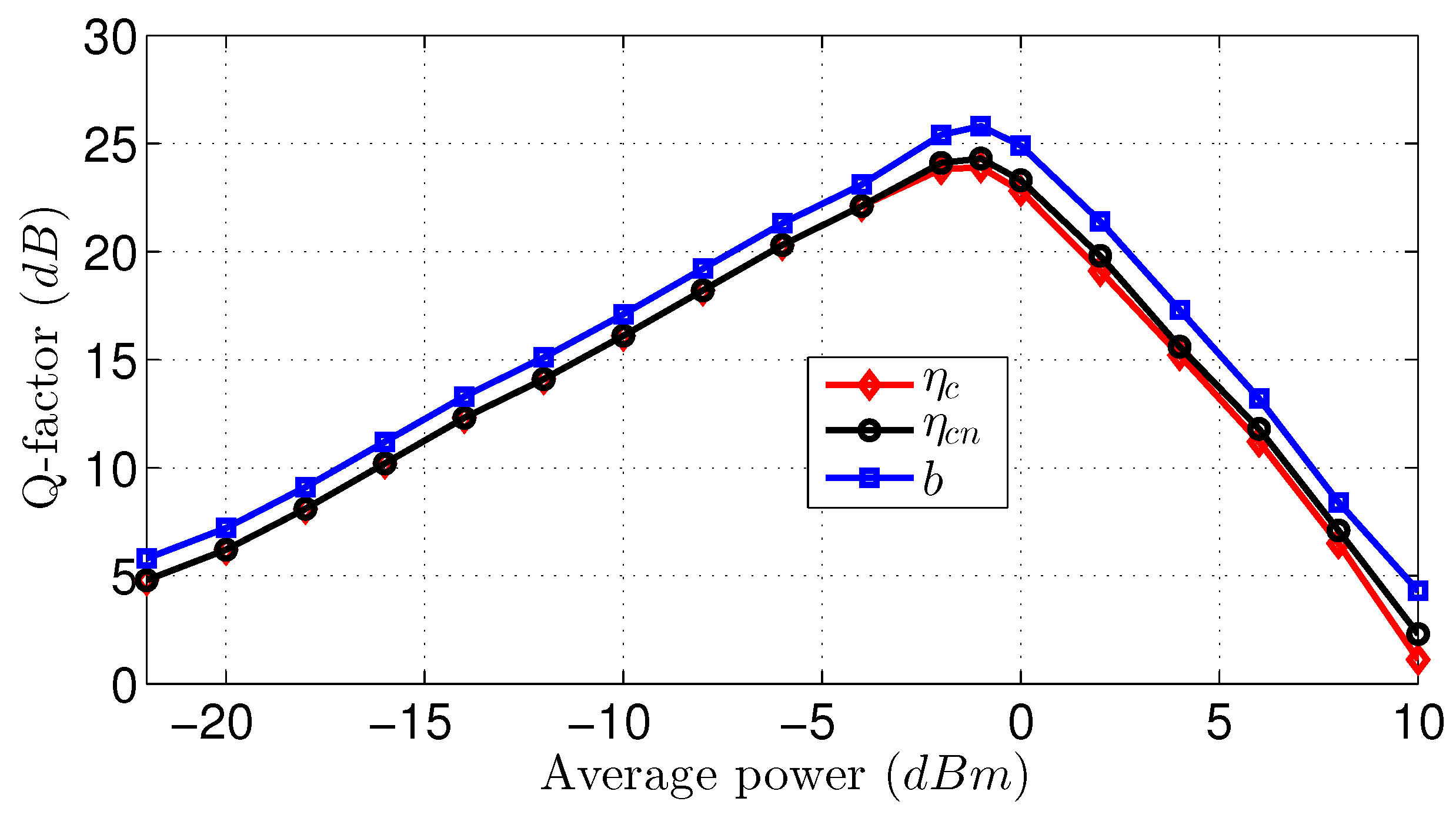
The local oscillator at the receiver side has no frequency drift and has a linewidth of 100 kHz. The total number of symbols transmitted was . We added of overhead to satisfy Step 1 of the direct NFT algorithm. An oversampling factor of 40 was selected for the simulations. The system performance for the three different modulations applying our algorithm are shown in Figure 6 and Figure 7. In Figure 6, we show the Q-factor versus the average power in the input of the optical fiber for all three modulations. We observe that the b-modulation performs better compared to the other two modulations, which on the other hand, show very similar performances. The maximum value of the Q-factor, Q = 25.9 dB, is achieved when the average power is equal to −1 dBm, for the b-modulation shown in the blue line in Figure 6. Compared to the other two modulations, the Q-factor is increased by 2 dB. If the average power is less than −1 dBm, the performance is deteriorating as the Q-factor is decreasing. The reason behind this is the noisy channel assumed in the system, which is added by the distributed optical Raman amplifiers assumed over the optical links. If the average power is greater than −1 dBm, then the Q-factor is also decreasing due to the nonlinear effects and the numerical errors from many approximation values in our method.
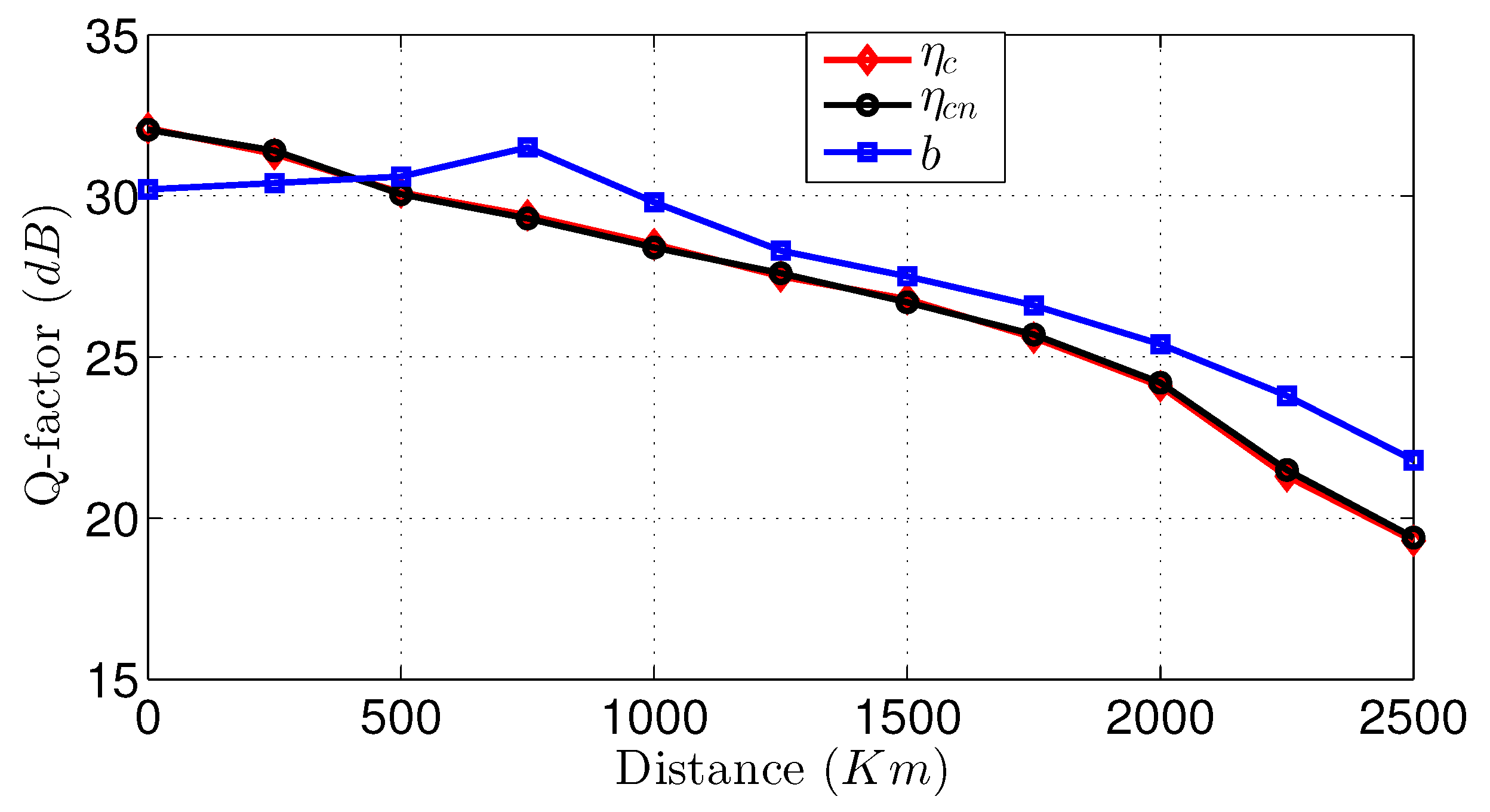
In Figure 7, we show the Q-factor versus transmission distances for all three modulations. We also observe better performance when b-modulation is used, shown in the blue line, and similar performances for the other two modulations. We observe that in the first 400 km of transmission distance, b-modulation has a lower Q-factor with respect to the other two. After 500 km of transmission distance, b-modulation start to shows a better Q-factor for all of the distances that we have simulated.
6. Conclusions
In this work, we have improved the NFT and INFT algorithms by going into the numerical details of the integral equation, proposing a novel methodology for their implementation, validating the results, and applying them on three different modulated signals for an optical communication system.
Only the continuous part of the nonlinear scattering data is investigated, as the spectral efficiency is higher and the complexity implementation is lower compared to the discrete nonlinear spectrum. We have considered the Boffetta-Osburne method for direct NFT, and the numerical solution of the GLM integral equation for INFT implementation. For both methods, we have simplified their complex mathematical derivation and have shown how to apply them step-by-step for an improved numerical implementation, as they are subject to various approximation errors that may drastically affect the final performance results.
We have identified four parameters that affect the performances of our numerical implementations of NFT and INFT during the validation process. They consist of two temporal parameters: T function width and M discrete points, and two spectral parameters: resolution in frequency and the number of points N. The temporal parameter, T, requires the function to be considered zero outside of , and this will be the source of additional overhead data that are used in a real modulated signal. The total discrete points, , will define how many data points we can transmit at the same time, similar to the OFDM scheme. A lower number will affect the performance of the system. The number of points N was selected to be a high number with the assumption of having a large oversampling factor at the transmitter side. All these parameters should be optimized in order to gain the maximum performance from the nonlinear Fourier transform. We also observed that for large amplitudes, the performance drastically decreased because when truncating the integrals, due to the Gibbs effect, the errors will also increase. In addition, during each iteration, the errors are accumulated by affecting the performance of the system. In Section 3.1, we showed the steps of the algorithm to be used to properly represent the signal in the time and frequency domains, and how we should select the domain of the Marchenko system for INFT implementation.
We then conducted extensive numerical simulations on three different modulation schemes. Our results suggest that b-modulation is an effective method to be used in optical fiber communication systems. It shows better performance with a higher Q-factor at a fixed input average power and distance.
The results presented in this paper show the feasibility of a continuous nonlinear optical-based spectrum with our proposed methodology for NFT/INFT implementation. Despite the fact that this is a significant step forward for numerical simulation, it needs further research targeting of least NFT/INFT complexity and higher accuracy algorithm. For future work, we plan to use only the Boffeta-Osburne method for both direct NFT and INFT using the duality principle, and we compare the results with a system where only the Marchenko system is used. Using only one algorithm without performance degradation will probably make the system less prone to numerical errors.
Author Contributions
Conceptualization, J.H. and E.D.; methodology, J.H.; software, J.H., E.D. and I.K.; validation, J.H. and W.H.F.A.; investigation, J.H. and M.A.; visualization, I.K. and E.D.; original draft preparation, J.H. and E.D.; review and editing, W.H.F.A. and M.A. All authors have read and agreed to the published version of the manuscript.
Funding
This research received no external funding.
Data Availability Statement
Not applicable.
Conflicts of Interest
The authors declare no conflict of interest.
References
- Winzer, P.J.; Neilson, D.T. From Scaling Disparities to Integrated Parallelism: A Decathlon for a Decade. J. Light. Technol. 2017, 35, 1099–1115. [Google Scholar] [CrossRef]
- Telegeography. Global Internet Geography. 2022. Available online: https://blog.telegeography.com/internet-traffic-and-capacity-remain-brisk (accessed on 1 October 2022).
- Agrell, E.; Karlsson, M.; Chraplyvy, A.R.; Richardson, D.J.; Krummrich, P.M.; Winzer, P.; Roberts, K.; Fischer, J.K.; Savory, S.J.; Eggleton, B.J.; et al. Roadmap of optical communications. J. Opt. 2016, 18, 063002. [Google Scholar] [CrossRef]
- Hoxha, J.; Shimizu, S.; Cincotti, G. On the performance of all-optical OFDM based PM-QPSK and PM-16QAM. Telecommun. Syst. 2020, 75, 355–367. [Google Scholar] [CrossRef]
- Yousefi, M.I.; Kschischang, F.R. Information Transmission Using the Nonlinear Fourier Transform, Part I: Mathematical Tools. IEEE Trans. Inf. Theory 2014, 60, 4312–4328. [Google Scholar] [CrossRef] [Green Version]
- Turitsyna, E.G.; Turitsyn, S.K. Digital signal processing based on inverse scattering transform. Opt. Lett. 2013, 38, 4186–4188. [Google Scholar] [CrossRef] [Green Version]
- Prilepsky, J.E.; Derevyanko, S.A.; Blow, K.J.; Gabitov, I.; Turitsyn, S.K. Nonlinear Inverse Synthesis and Eigenvalue Division Multiplexing in Optical Fiber Channels. Phys. Rev. Lett. 2014, 113, 013901. [Google Scholar] [CrossRef] [Green Version]
- Turitsyn, S.K. Nonlinear Fourier Transform for Optical Data Processing and Transmission: Advances and Perspectives. In Proceedings of the 2018 European Conference on Optical Communication (ECOC), Roma, Italy, 23–27 September 2018; pp. 1–3. [Google Scholar] [CrossRef] [Green Version]
- Yousefi, M.; Yangzhang, X. Linear and Nonlinear Frequency-Division Multiplexing. IEEE Trans. Inf. Theory 2020, 66, 478–495. [Google Scholar] [CrossRef] [Green Version]
- Yousefi, M.I.; Kschischang, F.R. Information Transmission Using the Nonlinear Fourier Transform, Part III: Spectrum Modulation. IEEE Trans. Inf. Theory 2014, 60, 4346–4369. [Google Scholar] [CrossRef] [Green Version]
- Taha, T.R.; Ablowitz, M.I. Analytical and numerical aspects of certain nonlinear evolution equations. II. Numerical, nonlinear Schrödinger equation. J. Comput. Phys. 1984, 55, 203–230. [Google Scholar] [CrossRef]
- Hasegawa, A.; Nyu, T. Eigenvalue communication. J. Light. Technol. 1993, 11, 395–399. [Google Scholar] [CrossRef]
- Meron, E.; Feder, M.; Shtaif, M. On the Achievable Communication Rates of Generalized Soliton Transmission Systems. arXiv 2012, arXiv:1207.0297. [Google Scholar]
- Hari, S.; Yousefi, M.I.; Kschischang, F.R. Multieigenvalue Communication. J. Light. Technol. 2016, 34, 3110–3117. [Google Scholar] [CrossRef]
- Dong, Z.; Hari, S.; Gui, T.; Zhong, K.; Yousefi, M.I.; Lu, C.; Wai, P.K.A.; Kschischang, F.R.; Lau, A.P.T. Nonlinear Frequency Division Multiplexed Transmissions Based on NFT. IEEE Photonics Technol. Lett. 2015, 27, 1621–1623. [Google Scholar] [CrossRef]
- Le, S.T.; Prilepsky, J.E.; Turitsyn, S.K. Nonlinear inverse synthesis for high spectral efficiency transmission in optical fibers. Opt. Express 2014, 22, 26720–26741. [Google Scholar] [CrossRef] [Green Version]
- Le, S.; Wahls, S.; Lavery, D.; Prilepsky, J.; Turitsyn, S. Reduced complexity nonlinear inverse synthesis for nonlinearity compensation in optical fiber links. In Proceedings of the European Conference on Lasers and Electro-Optics, Munich, Germany, 21–25 June 2015; Optica Publishing Group: Singapore, 2015; p. CI_3_2. [Google Scholar]
- García-Gómez, F.J. Communication Using Eigenvalues of Higher Multiplicity of the Nonlinear Fourier Transform. J. Light. Technol. 2018, 36, 5442–5450. [Google Scholar] [CrossRef] [Green Version]
- Span, A.; Aref, V.; Bülow, H.; Ten Brink, S. On time-bandwidth product of multi-soliton pulses. In Proceedings of the 2017 IEEE International Symposium on Information Theory (ISIT), Aachen, Germany, 25–30 June 2017; pp. 61–65. [Google Scholar] [CrossRef] [Green Version]
- Terauchi, H.; Maruta, A. Eigenvalue modulated optical transmission system based on digital coherent technology. In Proceedings of the 2013 18th OptoElectronics and Communications Conference held jointly with 2013 International Conference on Photonics in Switching (OECC/PS), Kyoto, Japan, 30 June–4 July 2013; pp. 1–2. [Google Scholar]
- Aref, V.; Bülow, H.; Schuh, K.; Idler, W. Experimental demonstration of nonlinear frequency division multiplexed transmission. In Proceedings of the 2015 European Conference on Optical Communication (ECOC), Valencia, Spain, 27 September–1 October 2015; pp. 1–3. [Google Scholar] [CrossRef] [Green Version]
- Buelow, H.; Aref, V.; Idler, W. Transmission of Waveforms Determined by 7 Eigenvalues with PSK-Modulated Spectral Amplitudes. In Proceedings of the ECOC 2016, 42nd European Conference on Optical Communication, Dusseldorf, Germany, 18–22 September 2016; pp. 1–3. [Google Scholar]
- Bülow, H.; Aref, V.; Schmalen, L. Modulation on Discrete Nonlinear Spectrum: Perturbation Sensitivity and Achievable Rates. IEEE Photonics Technol. Lett. 2018, 30, 423–426. [Google Scholar] [CrossRef]
- De Menezes, T.D.S.; Tu, C.; Besse, V.; O’Sullivan, M.; Grigoryan, V.S.; Menyuk, C.R.; Lima, I.T., Jr. Nonlinear Spectrum Modulation in the Anomalous Dispersion Regime Using Second- and Third-Order Solitons. Photonics 2022, 9, 748. [Google Scholar] [CrossRef]
- Yangzhang, X.; Lavery, D.; Bayvel, P.; Yousefi, M.I. Impact of Perturbations on Nonlinear Frequency-Division Multiplexing. J. Light. Technol. 2018, 36, 485–494. [Google Scholar] [CrossRef]
- Jones, R.T.; Gaiarin, S.; Yankov, M.P.; Zibar, D. Noise Robust Receiver for Eigenvalue Communication Systems. In Proceedings of the 2018 Optical Fiber Communications Conference and Exposition (OFC), San Diego, CA, USA, 5–9 March 2018; pp. 1–3. [Google Scholar]
- Civelli, S.; Forestieri, E.; Secondini, M. Why Noise and Dispersion May Seriously Hamper Nonlinear Frequency-Division Multiplexing. IEEE Photonics Technol. Lett. 2017, 29, 1332–1335. [Google Scholar] [CrossRef] [Green Version]
- Le, S.T.; Aref, V.; Buelow, H. High Speed Precompensated Nonlinear Frequency-Division Multiplexed Transmissions. J. Light. Technol. 2018, 36, 1296–1303. [Google Scholar] [CrossRef] [Green Version]
- Le, S.T.; Buelow, H.; Aref, V. Demonstration of 64x0.5Gbaud Nonlinear Frequency Division Multiplexed Transmission with 32QAM. In Proceedings of the Optical Fiber Communication Conference, Los Angeles, CA, USA, 19–23 March 2017; p. W3J.1. [Google Scholar] [CrossRef]
- Yangzhang, X.; Yousefi, M.I.; Alvarado, A.; Lavery, D.; Bayvel, P. Nonlinear Frequency-Division Multiplexing in the Focusing Regime. In Proceedings of the Optical Fiber Communication Conference, Los Angeles, CA, USA, 19–23 March 2017; p. Tu3D.1. [Google Scholar] [CrossRef] [Green Version]
- Goossens, J.W.; Yousefi, M.I.; Jaouën, Y.; Hafermann, H. Polarization-division multiplexing based on the nonlinear Fourier transform. Opt. Express 2017, 25, 26437–26452. [Google Scholar] [CrossRef] [PubMed]
- Leible, B.; Plabst, D.; Hanik, N. Back-to-Back Performance of the Full Spectrum Nonlinear Fourier Transform and Its Inverse. Entropy 2020, 22, 1131. [Google Scholar] [CrossRef] [PubMed]
- Xu, B.; Zhang, S. Analytical Method for Generalized Nonlinear Schrodinger Equation with Time-Varying Coefficients: Lax Representation, Riemann-Hilbert Problem Solutions. Mathematics 2022, 10, 1043. [Google Scholar] [CrossRef]
- Weideman, J.; Herbst, B. Finite difference methods for an AKNS eigenproblem. Math. Comput. Simul. 1997, 43, 77–88. [Google Scholar] [CrossRef]
- Ablowitz, M.J.; Ladik, J.F. Nonlinear differential–difference equations and Fourier analysis. J. Math. Phys. 1976, 17, 1011–1018. [Google Scholar] [CrossRef]
- Boffetta, G.; Osborne, A. Computation of the direct scattering transform for the nonlinear Schroedinger equation. J. Comput. Phys. 1992, 102, 252–264. [Google Scholar] [CrossRef]
- Osborne, A.R. Nonlinear Fourier Analysis: Rogue Waves in Numerical Modeling and Data Analysis. J. Mar. Sci. Eng. 2020, 8, 1005. [Google Scholar] [CrossRef]
- B, M.V.; Salle, M.A. Darboux Transformations and Solitons; Springer: Berlin, Germany, 1991. [Google Scholar]
- Prilepsky, J.E.; Derevyanko, S.A.; Turitsyn, S.K. Nonlinear spectral management: Linearization of the lossless fiber channel. Opt. Express 2013, 21, 24344–24367. [Google Scholar] [CrossRef] [Green Version]
- Wahls, S.; Chimmalgi, S.; Prins, P.J. FNFT: A Software Library for Computing Nonlinear Fourier Transforms. J. Open Source Softw. 2018, 3, 597. [Google Scholar] [CrossRef]
- Obaidat, S.; Mesloub, S. A New Explicit Four-Step Symmetric Method for Solving Schrödinger’s Equation. Mathematics 2019, 7, 1124. [Google Scholar] [CrossRef] [Green Version]
- Chen, J.; Zhang, Q. Ground State Solution of Pohožaev Type for Quasilinear Schrödinger Equation Involving Critical Exponent in Orlicz Space. Mathematics 2019, 7, 779. [Google Scholar] [CrossRef] [Green Version]
- Polyanin, A.D. Comparison of the Effectiveness of Different Methods for Constructing Exact Solutions to Nonlinear PDEs. Generalizations and New Solutions. Mathematics 2019, 7, 386. [Google Scholar] [CrossRef] [Green Version]
- Benia, Y.; Ruggieri, M.; Scapellato, A. Exact Solutions for a Modified Schrödinger Equation. Mathematics 2019, 7, 908. [Google Scholar] [CrossRef] [Green Version]
- Kosti, A.A.; Colreavy-Donnelly, S.; Caraffini, F.; Anastassi, Z.A. Efficient Computation of the Nonlinear Schrödinger Equation with Time-Dependent Coefficients. Mathematics 2020, 8, 374. [Google Scholar] [CrossRef] [Green Version]
- Wahls, S.; Poor, H.V. Fast Inverse Nonlinear Fourier Transform For Generating Multi-Solitons In Optical Fiber. arXiv 2015. [Google Scholar] [CrossRef]
- Wahls, S.; Poor, H.V. Introducing the fast nonlinear Fourier transform. In Proceedings of the 2013 IEEE International Conference on Acoustics, Speech and Signal Processing, Vancouver, BC, Canada, 26–31 May 2013; pp. 5780–5784. [Google Scholar] [CrossRef]
- Lax, P.D. Integrals of nonlinear equations of evolution and solitary waves. Commun. Pure Appl. Math. 1968, 21, 467–490. [Google Scholar] [CrossRef]
- Tataris, A.; van Leeuwen, T. A Regularised Total Least Squares Approach for 1D Inverse Scattering. Mathematics 2022, 10, 216. [Google Scholar] [CrossRef]
- Aricò, A.; Rodriguez, G.; Seatzu, S. Numerical solution of the nonlinear Schrödinger equation, starting from the scattering data. Calcolo 2011, 48, 75–88. [Google Scholar] [CrossRef]
- Gui, T.; Zhou, G.; Lu, C.; Lau, A.P.T.; Wahls, S. Nonlinear frequency division multiplexing with b-modulation: Shifting the energy barrier. Opt. Express 2018, 26, 27978–27990. [Google Scholar] [CrossRef] [Green Version]
- Wahls, S. Generation of Time-Limited Signals in the Nonlinear Fourier Domain via b-Modulation. In Proceedings of the 2017 European Conference on Optical Communication (ECOC), Gothenburg, Sweden, 17–21 September 2017; pp. 1–3. [Google Scholar] [CrossRef] [Green Version]
- Le, S.T.; Blow, K.J.; Menzentsev, V.K.; Turitsyn, S.K. Comparison of numerical bit error rate estimation methods in 112Gbs QPSK CO-OFDM transmission. In Proceedings of the 39th European Conference and Exhibition on Optical Communication (ECOC 2013), London, UK, 22–26 September 2013; pp. 1–3. [Google Scholar] [CrossRef]
Figure 1.
The soliton pulse defined in (55).
Figure 1.
The soliton pulse defined in (55).

Figure 2.
Real and imaginary parts of .

Figure 3.
Real and imaginary parts of .

Figure 4.
NMSEs of a() and b() for different values of M.

Figure 5.
The magnitude of in blue and in red.

Figure 6.
Q-factor versus input average power for all three modulations for a 50 Gbaud QPSK modulation over 1600 km of optical fiber. In blue line is shown the b-modulation; in black line, we show the modulation with a normalized reflection coefficient , given in Equation (64), and in red line, the normal modulation with reflection coefficient , given in Equation (63).

Figure 7.
Q-factor versus transmission distances for all three modulations for a 50 Gbaud QPSK modulation. In blue line is shown the b-modulation, in black line, we show the modulation with a normalized reflection coefficient given in Equation (64), and in red line, the normal modulation with reflection coefficient , given in Equation (63).

Publisher’s Note: MDPI stays neutral with regard to jurisdictional claims in published maps and institutional affiliations. |
© 2022 by the authors. Licensee MDPI, Basel, Switzerland. This article is an open access article distributed under the terms and conditions of the Creative Commons Attribution (CC BY) license (https://creativecommons.org/licenses/by/4.0/).
Share and Cite
MDPI and ACS Style
Hoxha, J.; Aly, W.H.F.; Dida, E.; Kertusha, I.; AlAkkoumi, M. A Novel Optical-Based Methodology for Improving Nonlinear Fourier Transform. Mathematics 2022, 10, 4513. https://0-doi-org.brum.beds.ac.uk/10.3390/math10234513
AMA Style
Hoxha J, Aly WHF, Dida E, Kertusha I, AlAkkoumi M. A Novel Optical-Based Methodology for Improving Nonlinear Fourier Transform. Mathematics. 2022; 10(23):4513. https://0-doi-org.brum.beds.ac.uk/10.3390/math10234513
Chicago/Turabian StyleHoxha, Julian, Wael Hosny Fouad Aly, Erdjana Dida, Iva Kertusha, and Mouhammad AlAkkoumi. 2022. "A Novel Optical-Based Methodology for Improving Nonlinear Fourier Transform" Mathematics 10, no. 23: 4513. https://0-doi-org.brum.beds.ac.uk/10.3390/math10234513
Note that from the first issue of 2016, this journal uses article numbers instead of page numbers. See further details here.