Modeling and Analysis of New Hybrid Clustering Technique for Vehicular Ad Hoc Network

Abstract

Many researchers have proposed algorithms to improve the network performance of vehicular ad hoc network (VANET) clustering techniques for different applications. The effectiveness of the clustering model is the most important challenge. The K-Means clustering algorithm is an effective algorithm for multi-clusters that can be used in VANETs. The problems with the K-Means algorithm concern the selection of a suitable number of clusters, the creation of a highly reliable cluster, and achieving high similarity within a cluster. To address these problems, a novel method combining a covering rough set and a K-Means clustering algorithm (RK-Means) was proposed in this paper. Firstly, RK-Means creates multi-groups of vehicles using a covering rough set based on effective parameters. Secondly, the K-value-calculating algorithm computes the optimal number of clusters. Finally, the classical K-Means algorithm is applied to create the vehicle clusters for each covering rough set group. The datasets used in this work were imported from Simulation of Urban Mobility (SUMO), representing two highway scenarios, high-density and low-density. Four evaluation indexes, namely, the root mean square error (RMSE), silhouette coefficient (SC), Davies–Bouldin (DB) index, and Dunn index (DI), were used directly to test and evaluate the results of the clustering. The evaluation process was implemented on RK-Means, K-Means++, and OK-Means models. The result of the compression showed that RK-Means had high cluster similarity, greater reliability, and error reductions of 32.5% and 24.2% compared with OK-Means and K-Means++, respectively.

1. Introduction

There is a need to tackle the problem of the recent increase in road accidents and traffic violations by implementing VANETs to exchange safety messages, broadcast and inform passengers of real-time traffic details, and provide many more roadside services. VANETs are self-organization networks that are part of mobile ad hoc networks (MANETs). A VANET has a more dynamically changing network topology that requires a flexible clustering model to avoid connection failure [1]. It creates a network of smart vehicles that communicate with each other. The communication is established via both dedicated short-range communication (DSRC) and/or mobile cellular networks [2]. The communication methods depend on the components of this network, whether they are vehicles or fixed units called road side units (RSUs). A VANET encompasses vehicle-to-vehicle (V2V) and vehicle-to-infrastructure (V2I) communications [3]. The clustering technique involves collecting neighboring nodes into clusters [4]. Different algorithms have different rules for creating clusters. The main VANET clustering scheme is shown in Figure 1. The connections between vehicles in the same cluster are called intra-cluster connections, and the connection between any two individual clusters is called an inter-cluster connection. The vehicles in a cluster are either cluster members (CMs), i.e., ordinary nodes, or the cluster head (CH), i.e., the cluster leader node.

VANET clustering techniques depend on the network topology. In a highway scenario, the most important parameters are the vehicle location, speed, and direction. In an urban scenario, the steering angle should be added as an important parameter. The cluster stability is calculated using either the average speed rate or the cluster changing rate. In [5], the number of status changes (NSC) of a vehicle during its participation in the network system was taken as the relationship between its speed and the vehicle transmission range. The cluster changing rate was computed in [6,7] to improve the cluster stability and select an optimal number of clusters. Converging cluster nodes and diverging the centroids of different clusters are two clustering algorithm challenges. The clustering algorithm proposed in this paper, RK-Means, creates a more stable clustering model with constraints on the average vehicle speed, therefore minimizing the intra-cluster distance (converging cluster nodes) and maximizing the inter-cluster distance (cluster divergence). The simulation results indicated that RK-Means outperformed the benchmark clustering models in the literature in terms of the evaluation by the unsupervised indexes RMSE, DB, DI, and SC, and cluster stability. The minimum value of standard deviation indicated that the proposed model has a small speed variant and that its cluster lifetime is higher than those of other algorithms.

The main contributions and innovations of this paper can be summarized as follows:

• A new K-Means clustering model based on a covering rough set is proposed to improve the cluster stability with minimum vehicle speed differences within clusters.
• The hybrid algorithm includes a new K-value calculation model to randomly enhance the attribution of data points and select an optimal number of clusters based on the minimum within-cluster error rate and vehicle coverage range.
• Five unsupervised evaluation indexes (RMSE, DB, DI, SC, and the standard deviation of speed) were used directly to evaluate and analyze the results of the clustering.
• Comparative tests were designed and executed to show the effectiveness of RK-Means. We selected two highway topology scenarios (high-density and low-density) and eight datasets, with constraints on the simulation time and vehicle density.

The rest of the paper is structured as follows: Section 2 summarizes the previous related studies. Section 3 introduces the system model. In Section 4, the evaluation model and indexes are described. Section 5 presents the simulation results and evaluates the performance of the proposed algorithm in comparison with two other algorithms based on the explained indexes. Finally, the conclusions and future research are presented in Section 6. The notations and acronyms used in this paper are shown in

Table 1. List of notations and acronyms.

Acronyms	Definition
CBL	Chain-Branch-Leaf
CG	Covering Group
CH	Cluster Head
CM	Cluster Member
CRS	Covering Rough Set
DB	Davies–Bouldin Index
DI	Dunn Index
DSRC	Dedicated Short-Range Communication
MANET	Mobile Ad Hoc Network
ML	Machine Learning
MPR	Multi-Point Relay Node
NSC	Number of Status Changes
OK-Means	Overlapping K-Means
OLSR	Optimized Link State Routing Protocol
RMSE	Root Mean Square Error
RSU	Road Side Unit
SC	Silhouette Coefficient
SUMO	Simulation of Urban Mobility
UAV	Unmanned Aerial Vehicle
V2I	Vehicle-to-Infrastructure Communications
V2V	Vehicle-to-Vehicle Communications
VANET	Vehicular Ad Hoc Network

.

2. Literature Study

Several articles have been devoted to the compilation of algorithms. In this section, we provide an overview of the previous literature and an analysis of its principles and technical limitations. Firstly, we explain the rough set clustering models that have been proposed for different applications.

Pawlak [8] proposed a new fuzzy set model to make decisions by the approximate inclusion of sets. The dataset is divided into upper and lower approximations. The rule decision can be implemented based on the upper or lower approximation depending on the application, and the boundary region can also be selected. Classical rough sets have the problems of difficulty dealing with real-value data and a low fault-tolerance level. The low tolerance level problem was solved in [9] by proposing a neighborhood rough-sets model to create variable-precision neighborhood approximation sets and positive regions, so the rough set becomes a dynamic model. The dynamic rough set model with the fuzzy scheme was used in [10] to make a more efficient rough set clustering system. This scheme enhances the rough set and implements it in a VANET dataset as a CH selection model. The CH selection model is created based on the node transmission range, and the vehicle is defined in a true cluster.

Regarding MANET applications, the authors of [11] proposed a rough set calibration scheme based on the node energy to classify the route and select the best route as an energy-efficient routing technique. The rough set calibration scheme ultimately makes use of episodic association for each parameter, including distance and energy. A new rough-set style was used in [12] to create a MANET clustering algorithm, and the main parameters for assigning the nodes to a true cluster were energy, delay, and bandwidth. The route classification model can classify the routes in a wireless network. The experimental route-classification results illustrate that this model has high accuracy compared with other algorithms.

Regarding healthcare data analysis, a CRS was used in [13] to enhance prediction, the initial identification of sicknesses, and disease classification by applying rough-set-based pattern classification techniques for healthcare data. For the diagnosis of diseases in different patients, the covering-based rough set classification provided more effective results than the delicate pattern classifier model. A novel neighborhood rough set classification approach was presented in [14] to deal with medical datasets. Five benchmarked medical datasets were used to study the impact of the neighborhood rough set classification approach on decision making. In [15], the dimension reduction of clusters was carried out based on a rough set to decrease the feature set of a decision system and improve the cluster performance. The application of the rough-set technique in VANETs represented a research gap, so the proposed model in this paper uses a CRS to create a covering group based on an effective VANET parameter to improve the K-Means clustering algorithm. Secondly, we explain the trends in clustering techniques and clustering based on K-Means by discussing different clustering models and K-Means clustering algorithms.

The Chain-Branch-Leaf (CBL) clustering algorithm proposed by [16] divides the VANET nodes into sectors and then creates a branch node as a cluster head and a leaf node as a normal node. The CBL algorithm was introduced to enhance the flooding of broadcast traffic and compared with the multi-point relay node (MPR) used in the Optimized Link State Routing protocol (OLSR). The CBL model has high stability in a high-speed VANET with location changes.

The K-Means clustering algorithm is used in various applications, including VANETs. The remainder of this section focuses on K-Means clustering models, with particular attention paid to their application in VANETs.

Regarding remote sensing applications, the authors of [17] used K-Means to select an optimum number of clusters (k) via a data-driven approach. They chose the optimum value of k from the value range (1 ≤ k ≤ 20), within which the true value was presumed to lie, and ran the K-Means clustering algorithm many times individually for each value of k. If the centroid values of all the tests were the same, they moved towards the new value of k, and this process was repeated for different sequence values of k until the centroid values of the clusters were found to be the same. The results were evaluated, and they obtained high cluster similarity.

In [18], the authors investigated an efficient clustering-based spectrum resource management scheme for dynamic heterogeneous vehicular networks. They proposed a low-complexity vehicle matching algorithm based on large-scale fading to improve the stability of communication links. In [19], the authors adjusted the well-known K-medoids algorithm to improve the stability of the network, and the lifetimes of all established links were increased. The cluster number and the initial CHs were not selected randomly, as is usual, but were based on a mathematical formula that considered the transmission ranges and the environment size and then assigned the nodes according to speed, proximity, directions, and other metrics. This metric prevented nodes with volatile and suspicious behavior from being selected as a new CH. The effectiveness of this model lies in its reduction of the cluster change rate in a highway scenario. In [20], a noise K-Means clustering algorithm was proposed to effectively solve the problems of computing the cluster numbers and the sensitivity of the clustering center initialization of the K-Means algorithm. The noise K-Means algorithm was applied to capture urban hotspots in big cities around the world. The authors of [21] suggested a modified K-Means algorithm and applied it with a Continuous Hopfield Network and Maximum Stable Set Problem for a VANET. The number of clusters was selected using the Maximum Stable Set Problem and Continuous Hopfield Network. Then, the distribution of vehicles to clusters was constrained by the link reliability model as a metric instead of the distance parameter that was used in the K-Means algorithm. The cluster member lifetime was increased, and the CH changing rate decreased. In [22], a location-based K-Means++ clustering algorithm was first developed to construct initial unmanned aerial vehicle (UAV) clusters. Subsequently, a weighted summation-based cluster head selection algorithm was proposed. The authors of [23] proposed an overlapping K-Means (OK-Means) clustering technique for a VANET based on overlapping clustering, and the number of clusters was calculated according to the node transmission range. The cluster length had to be less than two side-node transmission ranges. In [24], the authors proposed an entropy K-Means clustering algorithm that can be initialized without knowing the number of clusters and also demonstrates feature-reduction abilities. That is, the entropy K-Means algorithm can get rid of irrelevant features through feature reductions free of initializations by automatically finding the optimal number of clusters. The current paper proposes a model that uses more parameters, resulting in a more efficient clustering technique. The comparison results showed that the entropy K-Means algorithm can simultaneously find the optimal number of clusters and perform feature reduction.

This paper presents simulations and a comparison of results obtained for RK-Means, K-Means++ [22], and OK-Means [23].

RK-Means involves new criteria for selecting the initial number of clusters that are not included in K-Means++ and OK-Means. Furthermore, the use of a CRS in RK-Means increases the cluster stability compared with the other algorithms, because all cluster nodes have a minimum speed variant. The modified K-Means in the proposed RK-Means model attempts to collect the nodes with a minimum error rate. In low-density scenarios, there are large spaces between the clusters, so the proposed model provides high dissimilarity between clusters compared with other models. The challenge lies in high-density scenarios, which have small distances between clusters, and the proposed model was more successful at creating optimal clusters based on several parameters compared with the K-Means++ and OK-Means algorithms.

Table 2. RK-Means effective parameters compared with other clustering schemes in VANETs.

Proposed Model	Algorithm Type	Network Scenario	Effective Parameters
			Location	Speed	Direction	Distance	Transmission Range
CBL [16]	Single	Highway	√	√	˟	√	˟
K-Means [17]	Single	Satellite image	√	˟	˟	√	˟
Radio Resource [18]	Single	Highway	√	√	˟	√	√
Modified K-Means [21]	Hybrid	Highway	√	˟	˟	√	√
K-Means++ [22]	Single	UAV	√	˟	√	√	√
OK-Means [23]	Single	Highway	√	˟	√	√	√
RK-Means (proposed herein)	Hybrid	Highway	√	√	√	√	√

summarizes the effective parameters used in the discussed clustering schemes. From Table 2, we can observe that the proposed RK-Means scheme uses more parameters to create an efficient clustering technique and increase the cluster stability. The effective parameters considered were: node location and effectiveness in the clustering model; node speed; the direction of the node (because the direction parameter is more important in terms of cluster lifetime); node distance from reference location; and node transmission range (which indicates a node’s coverage in relation to other nodes and how it affects the cluster number). RK-Means includes all the above parameters, so the similarity within the clusters and the divergence between clusters are high.

3. Clustering Model

In this section, we present the proposed RK-Means clustering algorithm model, which comprises the following three main stages:

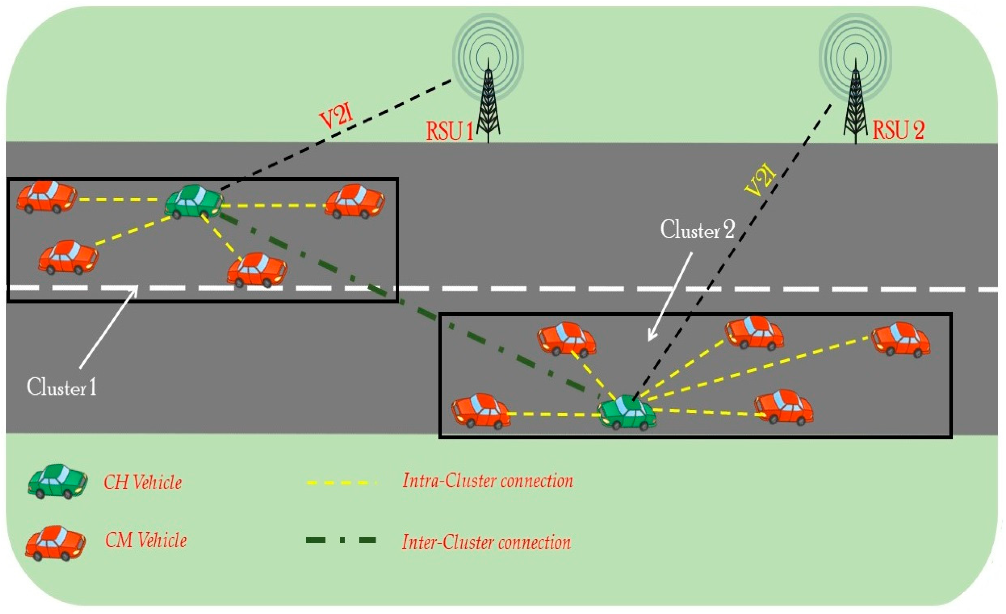
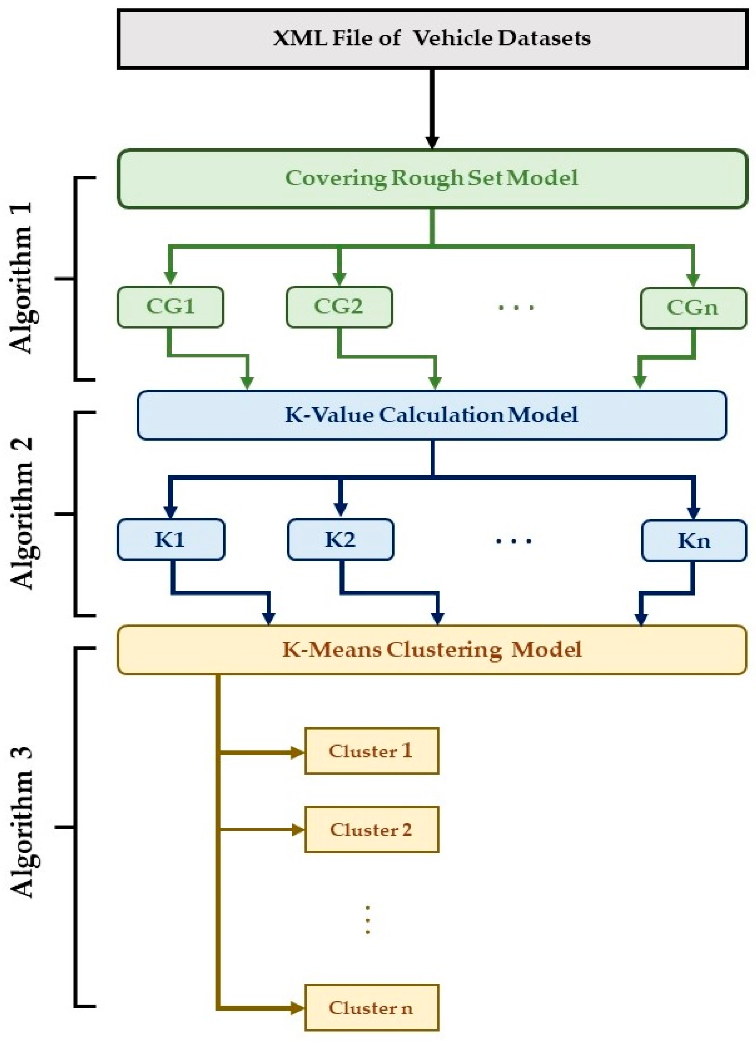
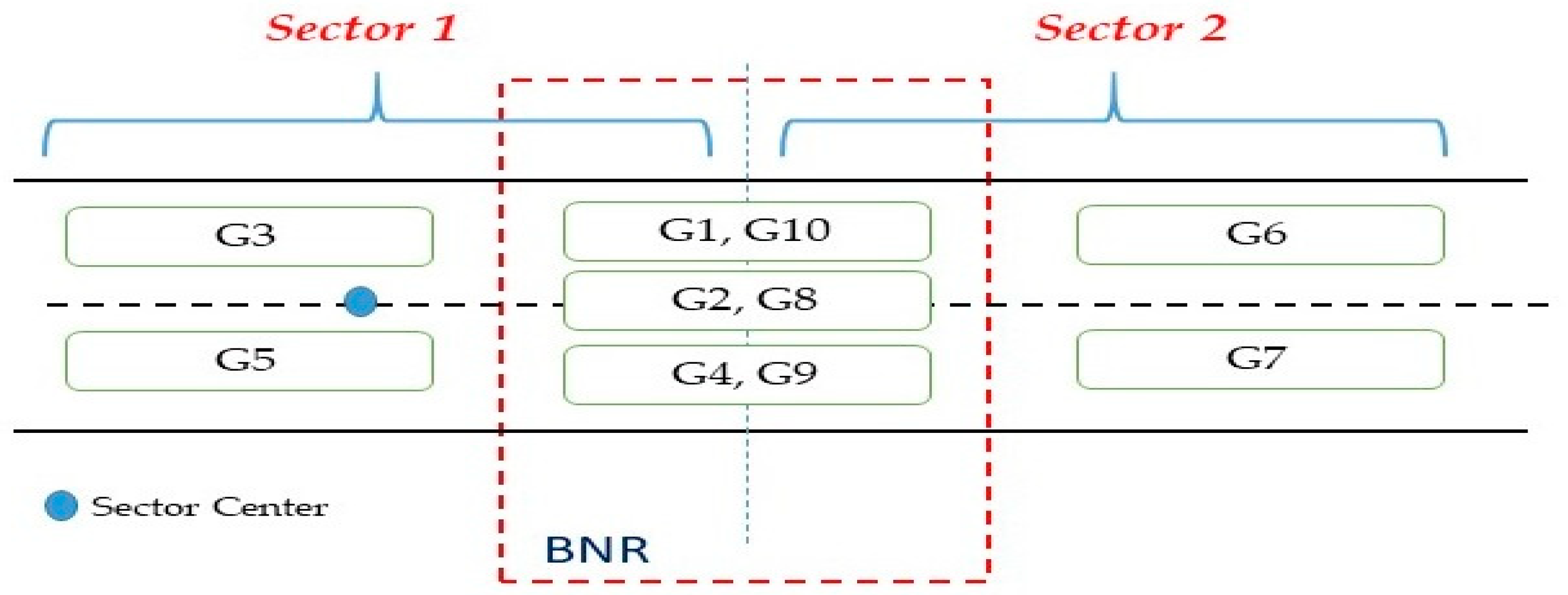
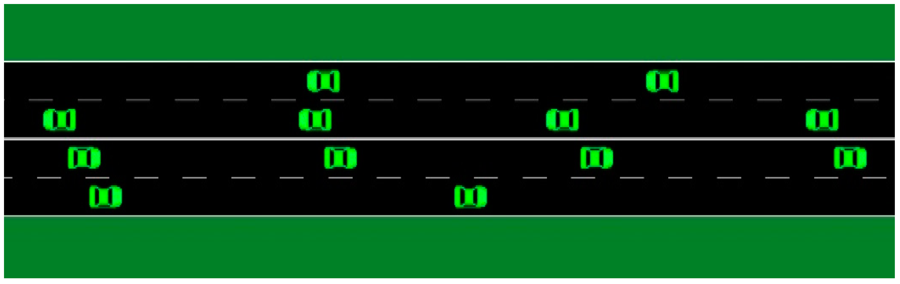
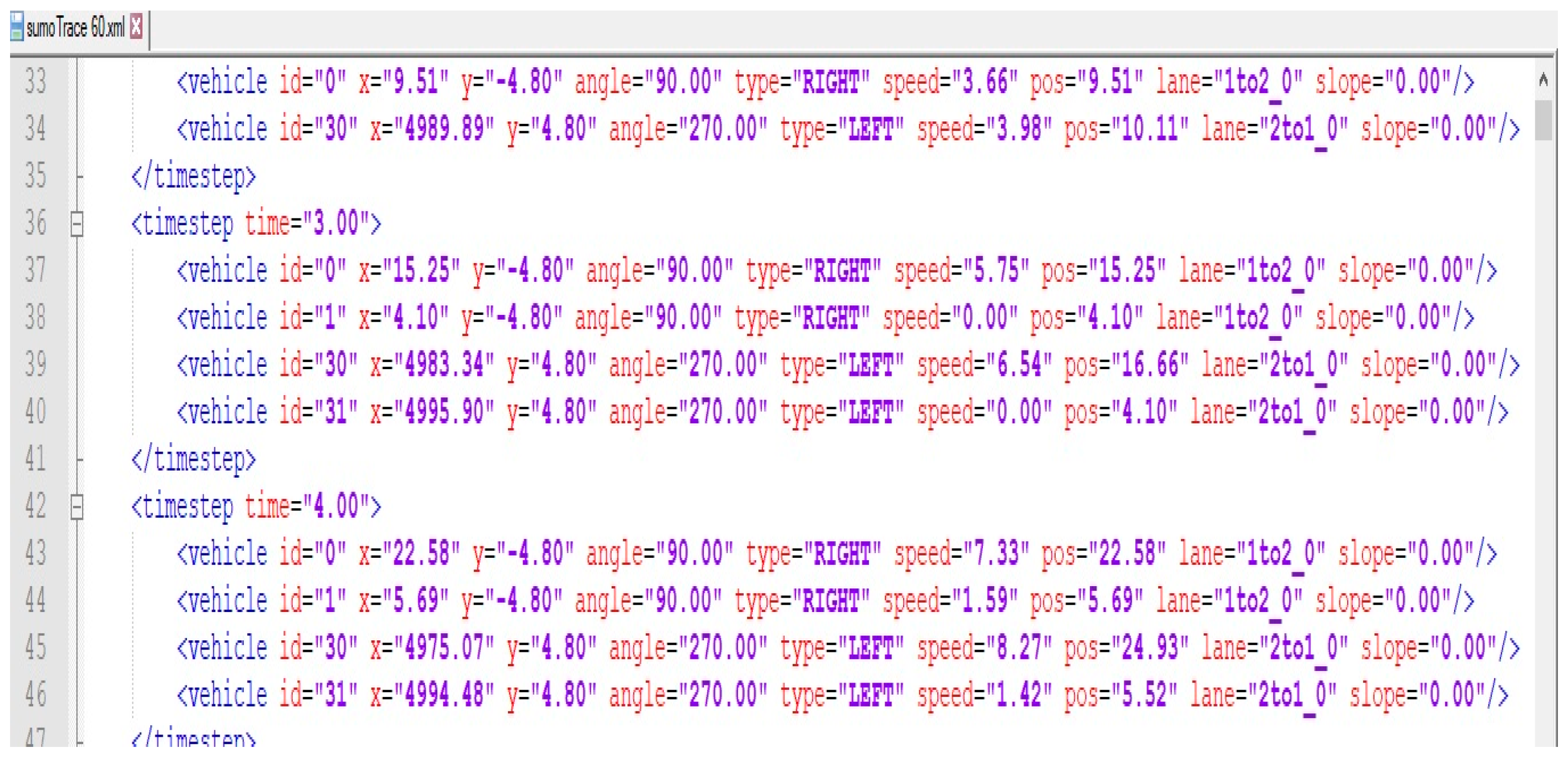
• Stage 1: The preparation of the datasets using SUMO software to collect the vehicle parameters at different timestamps. The XML file of the dataset describes the location, speed, direction, and steering angle. This study focused on a highway scenario, so the steering angle could not be used. To update this model for another scenario such as a city map, the steering angle would be a more important parameter to consider for covering table construction and clustering initialization. In this stage, the CRS algorithm works by considering all the vehicle parameters presented in the above table to initialize the covering groups. The covering groups divide the VANET datasets into multi-groups according to the approximation type. The output of the covering groups is CG1, CG2, CG3, …, and CGn. The number of covering groups depends on the vehicle status table and approximation types; in this paper, the number of groups was 10. The CRS model with descriptions of each step is illustrated in more detail in Section 3.1, where the main CRS algorithm includes the approximation calculation steps.
• Stage 2: In this stage, each covering group generated in stage 1 is input into the k-value calculation model to compute the number of clusters. At this stage, the optimal number of clusters is calculated based on two different models, and the minimum number of clusters is selected at the end. When the number of clusters has been calculated, the output represents the number of clusters in each covering group calculated in stage 1. The value of k1 represents the number of clusters in CG1, and the value of k2 is the number of clusters in CG2. For all covering groups in this work, the model generated the number of clusters. The cluster number calculation model is presented in detail in Section 3.2, with a description of the algorithm and each step.
• Stage 3: Finally, the cluster generation process is carried out by applying the classical K-Means clustering algorithm. The K-Means clustering algorithm creates the clusters of each covering group generated in stage 1 using the optimal cluster number calculated in stage 2. For example, if the value of k1 is 4, the K-Means algorithm creates four clusters from the CG1 datasets; if the k2 value is 6, it creates six clusters from CG2, and so on. This stage is explained in detail and the clustering algorithm is presented in Section 3.3.

The complete clustering model proposed in this work for vehicular ad hoc networks is shown in Figure 2.

3.1. Covering Rough Set Model

Pawlak [8] proposed a classical rough set based on the equivalence relation or segmentation of U, where the equivalence relation was changed to cover U in a CRS. The most important aspects of the rough set are the lower approximations, and the upper approximations of set X are shown in Figure 3.

The main goal of a CRS is to achieve a reasonable set of approximations and to reduce the number of attributes. The covering process is carried out based on symmetric relations, and distinctive reflexive relations are used to select the most useful vehicle states. Initially, an equivalence relation is created for the covering with the property that two elements intersect the union of finite element covering. A rough set is used to extract the rules and perform attribute reduction by partitions. Although CRS theory achieves the same function, the attributes are described by covers [25].

The steps of the rough set are as follows:

• Create an information table, which includes the general simulation parameters.
• Calculate the equivalence partition or relation for covering objects (denoted in this work by CG1, CG2, CG3,… CGn).
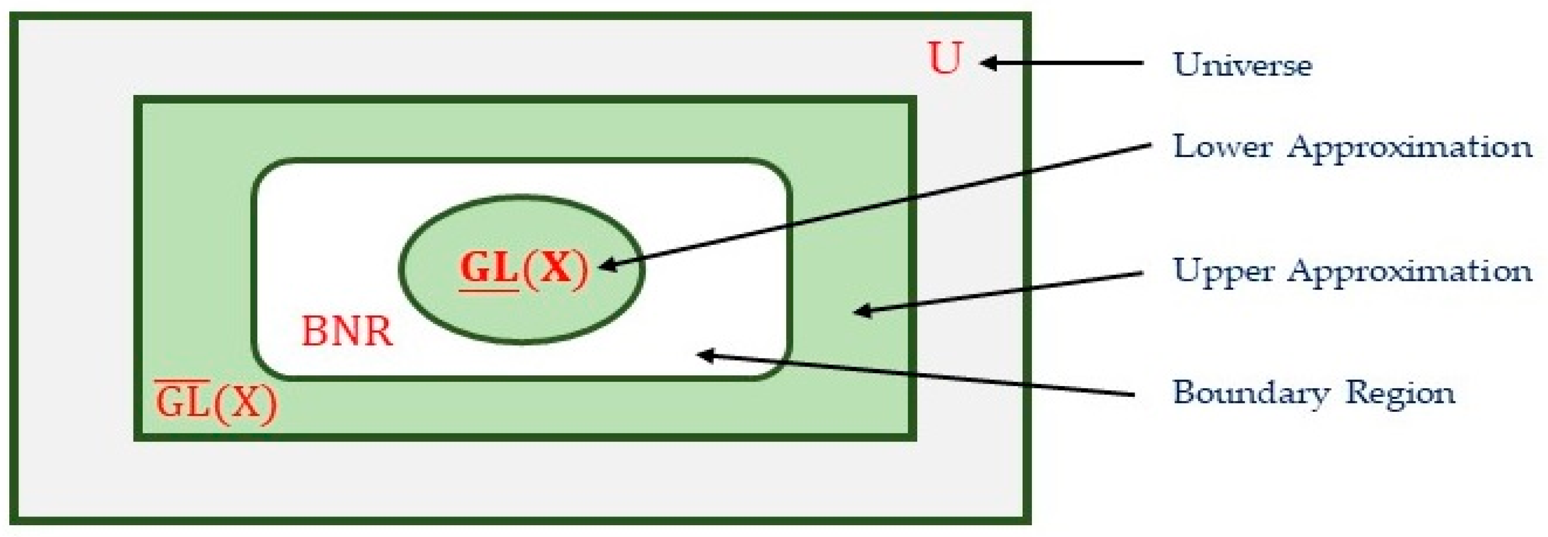
• Build the covering key of lower approximation for the given information table:

$$\underset{\_}{GL}\left(X\right)=\left\{k\left(x\right)\in GL:k\left(x\right)\subseteq X\right\}$$

(1)

• Build the covering key of the upper approximation for the given information table:

$$\overline{GL}\left(X\right)=\left\{{\displaystyle \cup }\left\{{\displaystyle \cap }\left\{k\in GL/x\in k\left(x\right)\right\}/x\in X\right\}\right\}$$

(2)

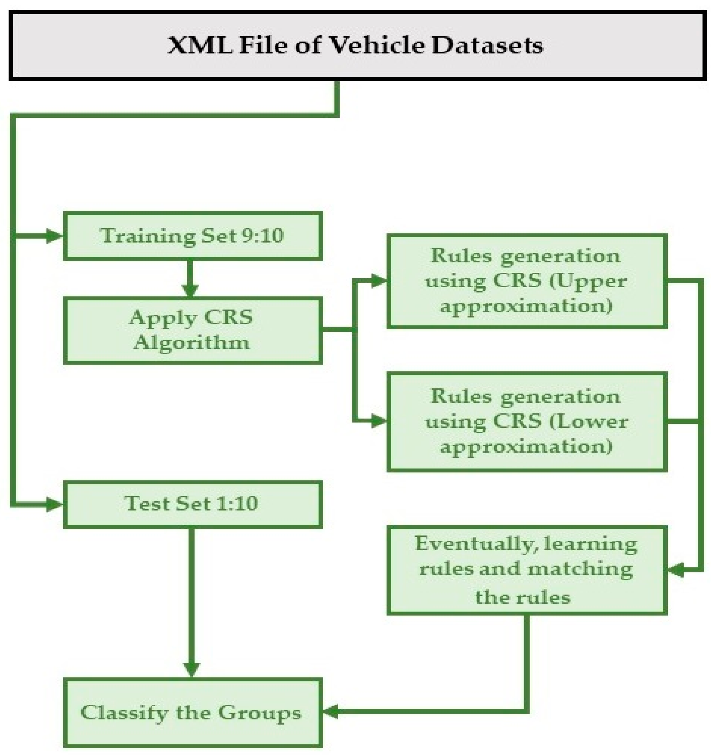
• Use CRS to build a certain rule based on (1).
• Use CRS to build possible rules based on (2).
• Eliminate an equivalent rule for covering approximations based on (3):

$$BNR=\underset{\_}{GL}\left(X\right)-\overline{GL}\left(X\right)$$

(3)

• Finally, calculate the validation measures, choose an appropriate group, and select the road sector.

Figure 4 shows the rough set system model that was used to collect vehicle groups.

3.1.1. Group Formation

In this subsection, the proposed grouping technique for the VANET clustering model based on CRSs is presented.

Definition 1.

Let the set of cases be U= {G1, G2, G3, ……, G10}, a set of conditional attributes be {Speed, Direction and Distance}, and a decision attribute be {Sector: CS and NS}, where CS denotes Current Sector and NS denotes Next Sector.

The speed and distance assumptions are defined by:

$$\{\begin{array}{cc}\hfill High Speed,& v\ge 22 m/s\\ \hfill Medium Speed,& 16\le v<22 m/s\\ \hfill Low Speed,& v<16 m/s\end{array}$$

(4)

$$\{\begin{array}{c}Distance \leftarrow Far, d_{C_i}^{V_i}>0.25 L\\ Distance \leftarrow Near, d_{C_i}^{V_i}\le 0.25 L \end{array}$$

(5)

where $d_{C_i}^{V_i}$ represents the distance between the vehicle and the center of the sector, and L is the total road length. The total number of sectors is two, each sector length is 0.5 L, and the distance between the sector center and the boundary virtual line is 0.25 L.

Table 3. Set of vehicle cases.

$\mathbf{U}\in \mathbf{A}$	Speed	Direction	Distance	Sector
G1	Medium	Right	Far	NS
G2	Low	Left	Near	CS
G3	Medium	Right	Near	CS
G4	High	Left	Near	CS
G5	High	Right	Near	CS
G6	Medium	Left	Far	NS
G7	Low	Right	Far	NS
G8	Low	Left	Near	NS
G9	High	Left	Near	NS
G10	Medium	Right	Far	CS

shows the set of vehicle cases.

According to Table 3, we can collect the groups as follows:

{Speed: Low} = {G2, G7, G8}

{Speed: Medium} = {G1, G3, G6, G10}

{Speed: High} = {G4, G5, G9}

{Direction: Left} = {G2, G4, G6, G8, G9}

{Direction: Right} = {G1, G3, G5, G7, G10}

{Distance: Far} = {G1, G6, G7, G10}

{Distance: Near} = {G2, G3, G4, G5, G8, G9}

Then, we can apply the covering rules to obtain the covering groups:

CG1 = Medium ∩ Right ∩ Far

CG1 = {G1, G3, G6, G10} ∩ {G1, G3, G5, G7, G10} ∩ {G1, G6, G7, G10}

    = {G1, G10}

CG2 = Low ∩ Left ∩ Near

CG2 = {G2, G7, G8} ∩ {G2, G4, G6, G8, G9} ∩ {G2, G3, G4, G5, G8, G9}

    = {G2, G8}

CG3 = Medium ∩ Right ∩ Near

CG3 = {G1, G3, G6, G10} ∩ {G1, G3, G5, G7, G10} ∩ {G2, G3, G4, G5, G8, G9}

    = {G3}

CG4 = High ∩ Left ∩ Near

CG4 = {G4, G5, G9} ∩ {G2, G4, G6, G8, G9} ∩ {G2, G3, G4, G5, G8, G9}

    = {G4, G9}

CG5 = High ∩ Right ∩ Near

CG5 = {G4, G5, G9} ∩ {G1, G3, G5, G7, G10} ∩ {G2, G3, G4, G5, G8, G9}

    = {G5}

CG6 = Medium ∩ Left ∩ Far

CG6 = {G1, G3, G6, G10} ∩ {G2, G4, G6, G8, G9} ∩ {G1, G6, G7, G10}

    = {G6}

CG7 = Low ∩ Right ∩ Far

CG7 = {G2, G7, G8} ∩ {G1, G3, G5, G7, G10} ∩ {G1, G6, G7, G10}

    = {G7}

CG8 = Low ∩ Left ∩ Near

CG8 = {G2, G7, G8} ∩ {G2, G4, G6, G8, G9} ∩ {G2, G3, G4, G5, G8, G9}

    = {G2, G8}

CG9 = High ∩ Left ∩ Near

CG9 = {G4, G5, G9} ∩ {G2, G4, G6, G8, G9} ∩ {G2, G3, G4, G5, G8, G9}

    = {G4, G9}

CG10 = Medium ∩ Right ∩ Far

CG10 = {G1, G3, G6, G10} ∩ {G1, G3, G5, G7, G10} ∩ {G1, G6, G7, G10}

    = {G1, G10}

Finally, the covering grouping formula is shown in (6).

CG = {{G1, G10}, {G2, G8}, {G3}, {G4, G9}, {G5}, {G6}, {G7}, {G2, G8}, {G4, G9}, {G1, G10}}

(6)

Definition 2.

Let {Sector: Current Sector} = {G2, G3, G4, G5, G1} and {Sector: Next Sector} = {G10, G6, G7, G8, G9}; then, by applying (1) and (2), the Covering rough set Lower approximation and Upper approximation are defined as:

$$\underset{\_}{GL}\left(X\right)=\{\begin{array}{c}\left\{G3, G5\right\}, Current Sector\\ \left\{G6, G7\right\}, Next Sector \end{array}$$

(7)

$$\overline{GL}\left(X\right)=\{\begin{array}{c}\left\{G1, G2, G3, G4, G5, G8, G9, G10\right\}, Current Sector \\ \left\{G1, G2, G4, G6, G7, G8, G9, G10\right\}, Next Sector \end{array}$$

(8)

By applying (3), we can compute the boundary region (BNR), as shown in (9):

$$BNR=\left\{G1, G2,G4, G8. G9.G10\right\}$$

(9)

The covering distribution is illustrated in Figure 5. Groups 1, 2, 4, 8, 9, and 10 are in the boundary region. The pairs {G1, G10}, {G2, G8}, and {G4, G9} are in the same featured group, and the clustering algorithm deals with them together.

3.1.2. Group Implementation

The CRS algorithm was applied to the training data based on vehicle cases. The CRS algorithm was explained in Algorithm 1. Eventually, according to the rule decision, a rule is chosen for further processing. In this paper, we used a 10-fold cross that comprised 90% data for training and 10% data for testing.

Algorithm 1 Implementation of CRS

Initialize v.id, v.location, v.speed ← read from the dataset v.direction ← {1,2}//1 for left, 2 for right L ← road length, c1 ← sector center RSU1 ← (xrsu1,yrsu1), RSU2 ← (xrsu2,yrsu2) begin for i = 1 to n do $d_{c{1}_i}^{v. x_i}=\sqrt{{\left(v.x\left(i\right)-c1\left(x\right)\right)}^2+{\left(v.y\left(i\right)-c1\left(y\right)\right)}^2}$ Distance (i) ← {near, far} based on the value of L and Formula (5) Compare v.speed(i) with the range of speed Speed (i) ← {high, medium, low} based on Formula (4) Direction (i) ← {left, right} based on v.direction input Calculate the distance between the vehicle and {RSU1, RSU2} then assign the decision-making {CS, NS} end for for i = 1 to n do Apply the rule in Table 1 to create G = {G1, G2, G3, …, Gn} end for for i = 1 to n do Create the covering groups using Formula (6)//CG1, CG2, CG3, …, and CGn Select the Upper and Lower Approximation using Formula (1) and Formula (2) Calculate the Boundary Region using Formula (3) end for Export the CG and Boundary Region end

3.2. K-Value Calculation Model

In this subsection, we try to select an optimal number of clusters (optimal K value). In the traditional K-Means clustering algorithm, the k-value selection is based on the minimum error rate only. The error rate can be calculated as the minimum value of cluster distance. In this work, we propose a different procedure to calculate the value of K.

Procedure steps

• Calculate the initial value of K.

Definition 3.

Let CG= {v₁,v₂,…,v_n} be a set of group vehicles imported from CRS and VL={(v₁.x,v₁.y),(v₂.x,v₂.y), … (v.xn,v.yn)} be a set of Vehicle Locations. If and only if VL $\in$the vehicle group and not accessed in the group boundary, then:

d_Max is the maximum distance within the group, and the representative group length can be defined as:

$$d_{Max.}=Mix\left\{d\left(V_i, V_j\right)\right\}$$

(10)

Let CR be the node coverage region; then, K* is:

$$K^{*}=\frac{d_{Max.}}{CR}$$

(11)

where K* is the initial value of K.

• Calculate the second value of K based on the similarity matrix.

The second step in this procedure is to select a random K value, implement the K-Means clustering algorithm, and then calculate the similarity matrix and change the K value several times to obtain a minimum error rate. The second value of K is K**.

Definition 4.

Let {v₁,v₂,…,vn} be a set of cluster vehicles and VL = {(v₁.x,v₁.y), (v₂.x,v₂.y), … (v.xn,v.yn)} be the set of Vehicle Locations. If and only if∀vehicles $\in$C, the similarity matrix represents the within-cluster distance (WD) matrix and is defined by:

$$WD=\left[\begin{array}{ccccc} 0& & & & \\ d\left(2,1\right)& 0& & & \\ d\left(3,1\right)& d\left(3,2\right)& 0& & \\ ⋮& ⋮ & ⋮ & 0 & \\ d\left(n,1\right)& d\left(n,2\right)& d\left(n,3\right)& \dots & 0\end{array}\right]$$

(12)

The sum square of the error (SSE) is the total summation of all rows in the WD matrix. The SSE can be computed as:

$$SSE={\displaystyle \sum }_{i=1}^n{\displaystyle \sum }_{j=1}^{n}d{\left(v_i,v_j\right)}^2$$

(13)

where $d\left(v_i,v_j\right)=\sqrt{{\left(x\left(i\right)-x\left(j\right)\right)}^2+{\left(y\left(i\right)-y\left(j\right)\right)}^2}$.

Figure 6 shows the K** calculation flowcharts concerning the value of the SSE. The K** calculation model comprises the following steps:

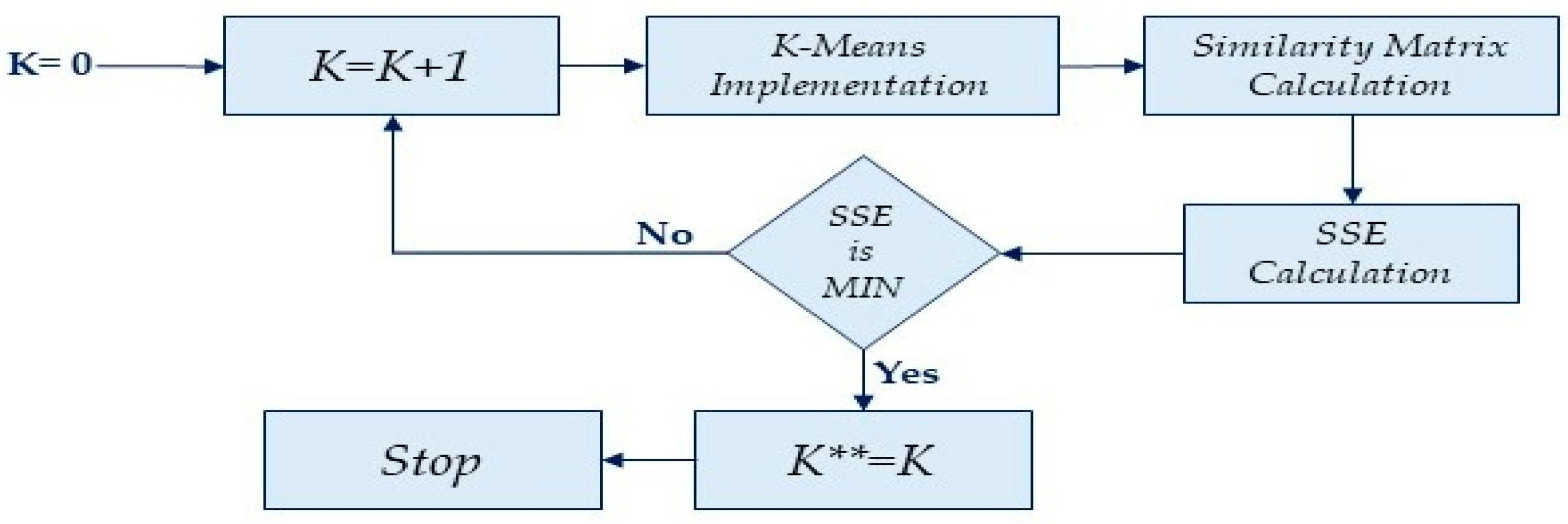
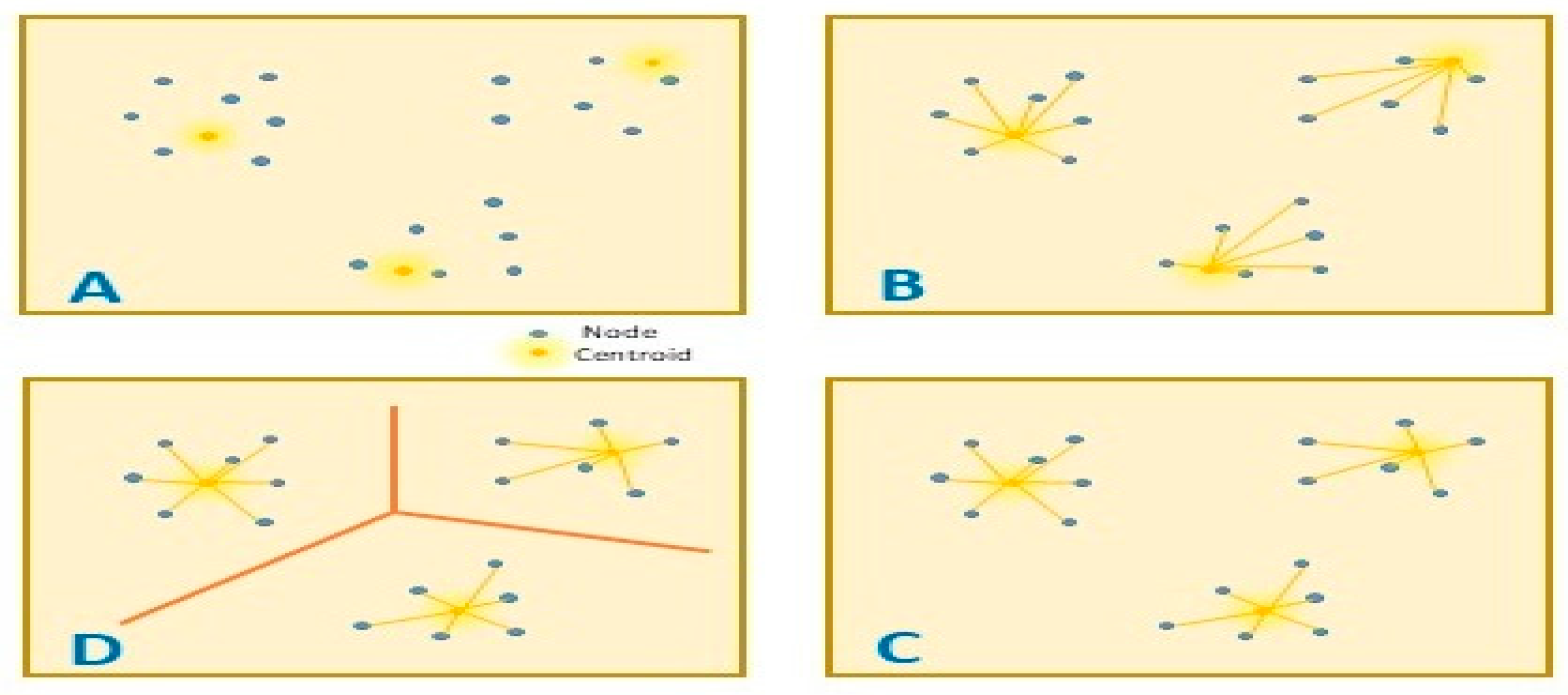
• Select k = 0, then increase the value of k.
• Apply the K-Means clustering algorithm.
• Calculate the cluster similarity based on (12) and (13).
• Check the error rate value; if the value is at its minimum, then stop.
• For each high error value, increase the value of k and repeat steps 2 to 4.

Figure 6. K** calculation flowchart.

Figure 6. K** calculation flowchart.

• Compute the final value of K.

Finally, the clustering K-value is obtained as in (14) by selecting the minimum value of K. The initial K* value and the second K** value are compared, and the optimal value is computed. Algorithm 2 shows the K value of the proposed model for a VANET in a highway scenario.

$$K=min\left(K^{*},K^{**}\right)$$

(14)

Algorithm 2 K-value calculation

Initialize G, N, X, Y, R//G: a group of vehicles, n: number of vehicles in each group, X, Y: vehicle locations, CR: vehicle coverage area. begin for all nodes do Calculate the distance among all vehicles groups; dMax.← maximum distance//Calculate the group length end for Calculate K* as the nearest integer greater value using equation (11) Select a random number of k for S = 1 to K do K** = S + 1; for i = 1 to n do Initialize centroid Ci based on K** Assign other vehicles to Ci Apply Equations (12) and (13) to calculate SSE end for SSE(s) = SSE; // calculate SSE for each group. end for for S = 1 to K do Compute the minim value of SSE K** ← S; end for Use Equation (14) to select K Export K; end

3.3. K-Means Model

The K-Means algorithm is the most important algorithm in the clustering steps and is used in various fields, such as data mining, wireless sensor networks, and ad hoc networks. An unsupervised machine learning (ML) technique classifies the dataset as a group of fixed K clusters at the start of the algorithm procedure. The main objective is to minimize the member distance and the CHs. As mentioned in Figure 7A, the algorithm chooses the initial K value (for example, three clusters), and the blue node represents the cluster member with a yellow centroid location that was initially selected. The objective is to assign the set of vehicles $v_j$ with 1 ≤ j ≤ N into K clusters. K-Means randomly chooses K points v_i with 1 ≤ i ≤ K of data in the vehicle dataset as cluster centroids, where each cluster centroid belongs to cluster C. Then, the algorithm collects each point in the vehicle dataset to the nearest cluster centroid. This process is conducted according to an objective function, which computes the sum of all squared distances between the CMs and the centroids in all clusters, as shown in Figure 7b. This is the second iteration to choose an optimal centroid location for each cluster, and the calculation is applied using the objective function (15):

$$avgmi{n}_c{\displaystyle \sum }_{i=1}^k{\displaystyle \sum }_{v_j\in C_i}d(v_j,u_i)=avgmi{n}_c{\displaystyle \sum }_{i=1}^k{\displaystyle \sum }_{v_j\in C_i}{\left|v_j-u_i\right|}^2$$

(15)

where $d\left(v_j,u_i\right)$ is the vehicle to cluster centroid Euclidean distance; $v_j$ is the vehicle position and $u_i$ is the cluster centroid position with i = 1, …, K; and K is the number of clusters. After assigning the vehicles in each cluster with the optimal centroid location, as shown in Figure 7c, the K-Means algorithm updates the position of each cluster centroid as the average distance between each node and cluster centroid using (16):

$$u_i=\frac{1}{\left|C_i\right|}{\displaystyle \sum }_{j\in C_i}{v}_j , \forall i$$

(16)

Finally, the clusters are formed with the minimum within-cluster distance, as shown in Figure 7d. When the final centroid location has been calculated and the minimum distance has been computed, and all nodes are in the centroid region.

The global algorithm is illustrated in Algorithm 3; the main goal of this algorithm is to create clusters using the optimal K value. The main steps of this algorithm can be summarized as follows:

Import the value of K from Algorithm 2.

Select the initial centroid for each cluster.

Assign all vehicles to the nearest centroid to create clusters.

Compute a new cluster centroid based on (16).

Repeat steps 3 and 4 to obtain the optimal centroid location.

Ensure that all vehicles have been assigned to clusters.

Algorithm 3 K-Means Implementation

Initialize Number of cluster centroids k; Set of vehicles N; List of cluster centroids assigned Ck begin Repeat for each vehicle in N do Compute the vehicles to the cluster centroid of ith cluster distance based on Equation (15) Assign each vehicle to the nearest cluster centroid. end for for each cluster do Compute the new cluster centroid position based on Equation (16). end for Until all vehicles belong to a cluster or the maximum number of iterations is reached end

4. Problem Formulation and Evaluation Model

4.1. Problem Formulation

The most important problem in data mining is data clustering. The clustering technique can be used in various fields, including ad hoc networks. The clustering technique should distribute the nodes as clusters with high similarity. An efficient clustering model has to verify the following:

• Maximizing the intra-cluster similarity by minimizing the distances between vehicles in the same cluster.
• Minimizing inter-cluster similarity by maximizing the distances between vehicle clusters.

There are many indices for evaluating cluster efficiency. In this work, we used the most popular indices to evaluate the proposed clustering algorithm and then compared the results with other clustering algorithms in the VANET field.

4.2. Similarity Measurement

A similarity measurement can be defined as the distance between cluster vehicles. While similarity is a value that illustrates the strength of the relationship between two vehicles, dissimilarity deals with the measurement of divergence between two vehicles. The performance of different algorithms depends on how they select an effective distance function for the input dataset. The Root Mean Square Error (RMSE) [26] was used to check the clustering similarity.

$$RMSE=\sqrt{\frac{1}{n}{\displaystyle \sum }_{i,j=1}^n{\left(d\left(v_i,v_j\right)\right)}^2}$$

(17)

where x_i and v_i are two vehicles, and n is the number of vehicles in the cluster. RMSE calculates the square root of the average distance between all vehicles in the existing cluster. A small RMSE represents high cluster similarity.

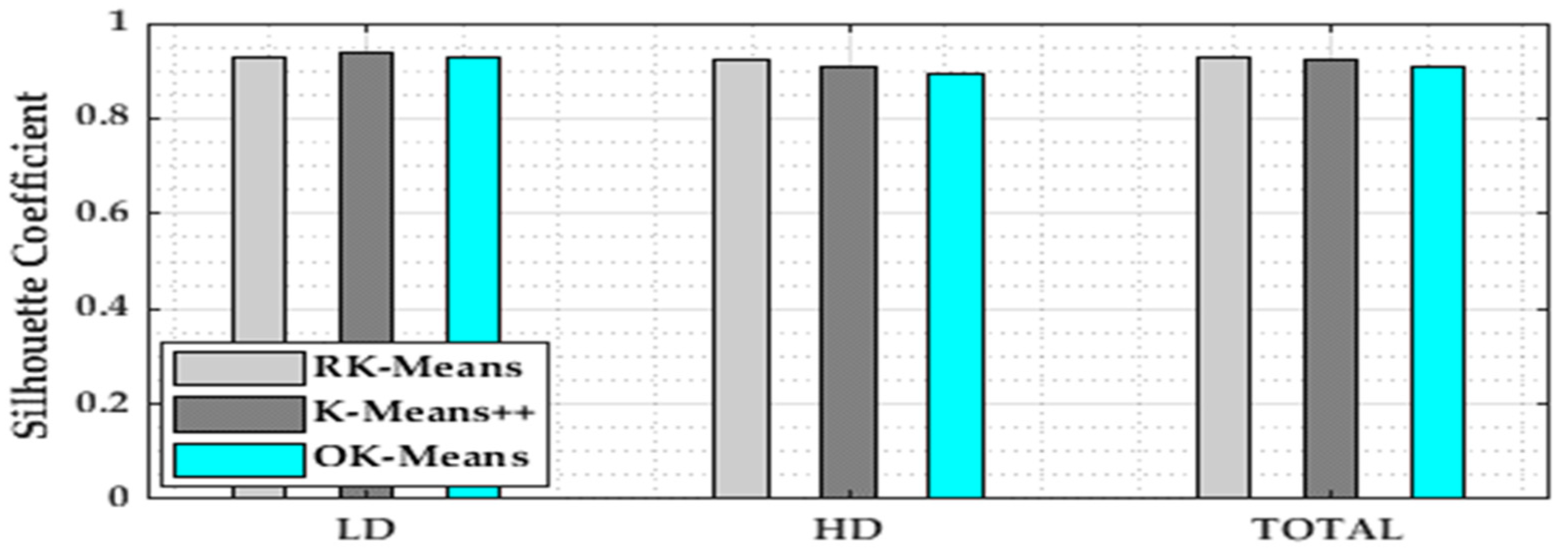
4.3. Silhouette Coefficient (SC)

The Silhouette Coefficient (SC) represents the fit of objects within a cluster. The quality of a cluster can be measured in the range of −1 to 1. A value that is near one (1) indicates that the vehicle belongs to the right cluster. This coefficient involves the two terms of cohesion and separation. Cohesion is the intra-clustering distance, and separation is the distance between cluster centroids. A(x) is the average distance between the sample vehicle and all other vehicles in the same cluster. B(x) is the average distance between the sample vehicle and all other vehicles in its nearest cluster. A value near −1 for a cluster indicates that the vehicles should belong to another cluster. The SC can be computed as follows [27]:

$$A\left(x\right)=\frac{1}{n_i-1}{\displaystyle \sum }_{v_i\in C_i}d\left(v_{sample},v_i\right)$$

(18)

$$B\left(x\right)=min\left\{\frac{1}{n_j}{\displaystyle \sum }_{v_j\in C_j}d\left(v_{sample},v_j\right)\right\}$$

(19)

$$SC\left(i\right)= \frac{B\left(x\right)-A\left(x\right)}{max\left\{B\left(x\right),A\left(x\right)\right\}}$$

(20)

where $v_{sample}$ is the vehicle sample; $v_i$ is the clustered vehicle; $d\left(v_{sample},v_i\right)$ represents the Euclidean distance between the sample vehicle and all vehicles in the same cluster; and $d\left(v_{sample},v_j\right)$ represents the Euclidean distance between the sample vehicle and all vehicles in the closest cluster. Based on the value of A and B, we can rewrite the Formula (20) as:

$$SC\left(i\right)=\{\begin{array}{c}1-\frac{A\left(x\right)}{B\left(x\right)}, A\left(x\right)<B\left(x\right) \\ 0, A\left(x\right)=B\left(x\right) \\ \frac{B\left(x\right)}{A\left(x\right)}-1, A\left(x\right)>B\left(x\right) \end{array}$$

(21)

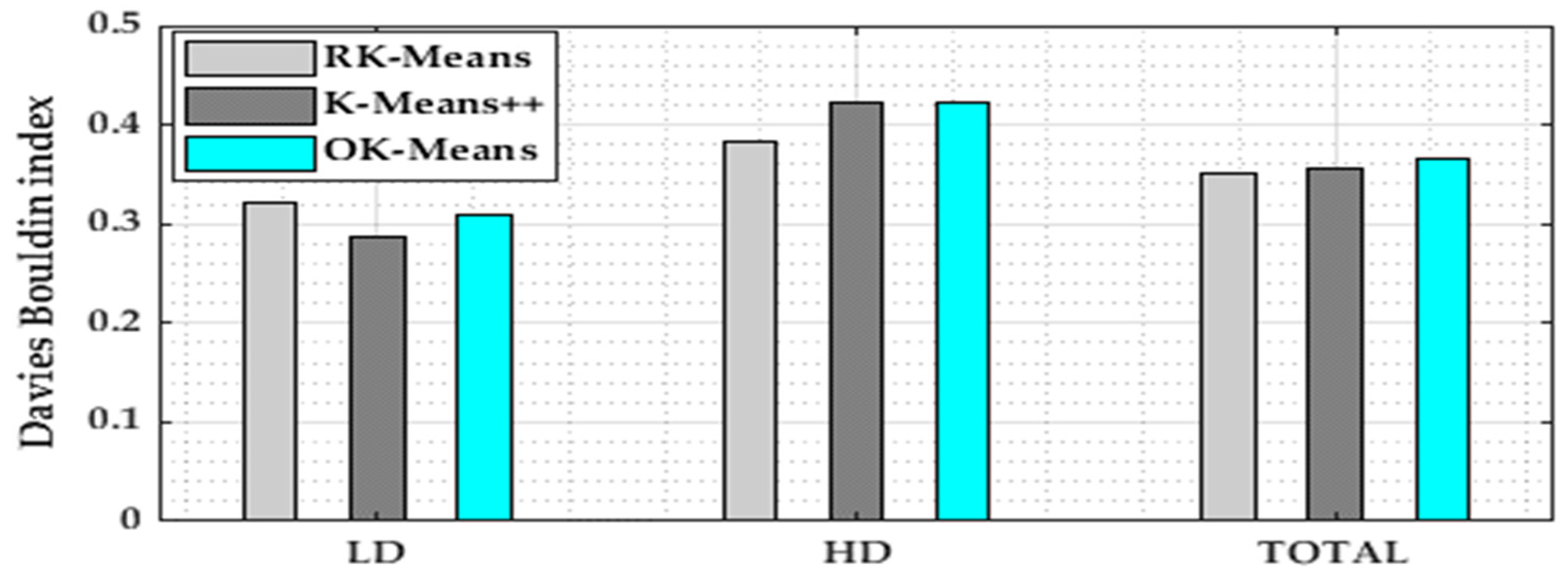
4.4. Davies–Bouldin Index

The Davies–Bouldin (DB) index is the measurement of the average similarity between each cluster and the most similar one. A lower DB index value indicates that the clustered vehicles have converged and the divergence of clusters is high. The goal of the DB index is to achieve minimum within-cluster variance and maximum between-cluster separation. It measures the similarity of a cluster ($R_{ij}$) according to its variance ($Si$) and the separation of a cluster ($d_{ij}$) according to the distance between two clusters ($C_i and C_j$). The formulae of the DB index are [28]:

$$Si=\frac{1}{ni}{\displaystyle \sum }_{v\in ci}d{\left(v_i,v_k\right)}^2$$

(22)

$$d_{ij}=d\left(C_i,C_j\right)$$

(23)

$$R_{ij}=\frac{Si+Sj}{d_{ij}}$$

(24)

$$R_i=max\left(R_{ij}\right), i\ne j, 0\le j<n_c$$

(25)

$$DB=\frac{1}{n_c} {\displaystyle \sum }_{i=1}^{n_c}{R}_i$$

(26)

where:

• $n_c$: Number of total clusters;
• $ni$: Number of vehicles in the i^th cluster;
• $C_i$: Value of the center of the i^th cluster;
• $d\left(C_i,C_j\right)$: Euclidean distance between two centers;
• $v_i \mathrm{and} v_k$: Two vehicles in the i^th cluster.

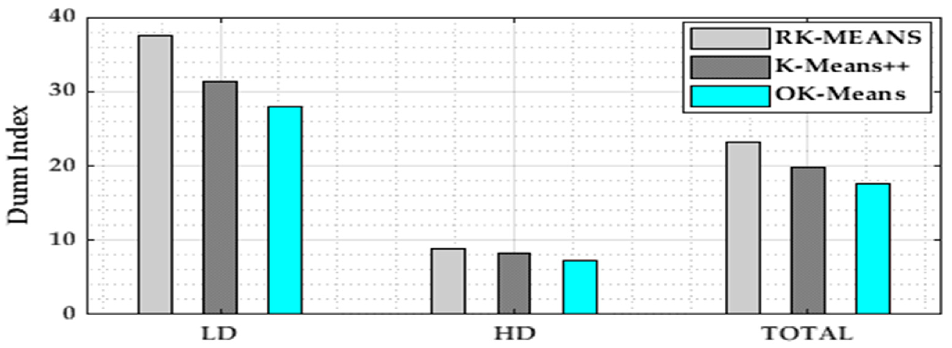
4.5. Dunn Index

The Dunn index (DI) is an index used to calculate the clustering similarity. The DI value is high if the vehicle clusters are well-separated. If the vehicles are in compact and well-separated clusters, the distance between any two clusters is expected to be high, and the cluster diameter is expected to be small. Clusters are compact and well-separated when the inter-cluster distance is maximized and the intra-cluster distance is minimized. A large DI value indicates compact and well-separated clusters. The formulae of the DI are [26]:

$$d\left(C_i,C_j\right)=\left\{d\left(cente{r}_i,cente{r}_j\right)\right\}$$

(27)

where $cente{r}_i \mathrm{and} cente{r}_j$ are the centroids of two clusters;

$$diam\left(C_i\right)=max\left\{d\left(v_i,v_k\right)\right\}$$

(28)

where $v_i \mathrm{and} v_k$ are two vehicles in the same cluster;

$$DI=\frac{min\left(d\left(C_i,C_j\right)\right)}{diam\left(C_i\right)}$$

(29)

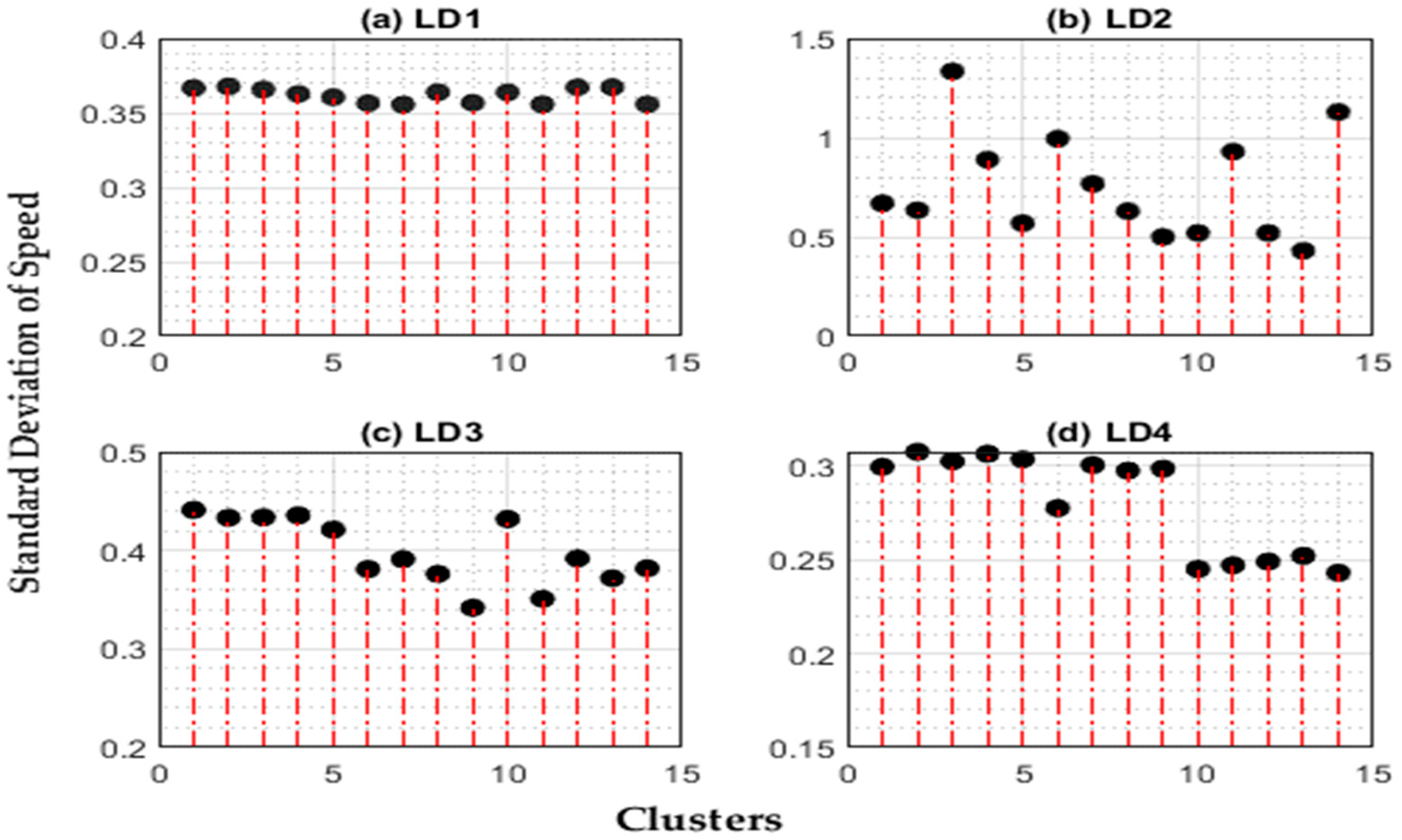
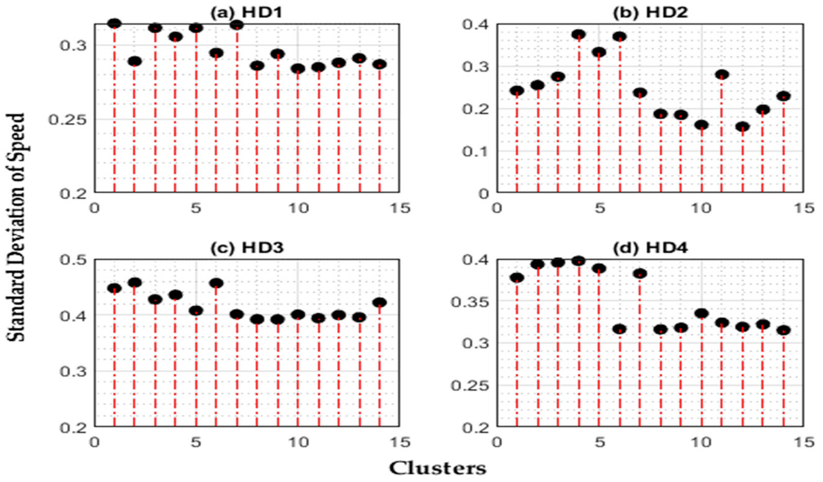
4.6. Cluster Speed Stability

The cluster speed is most important for explaining the cluster lifetime. When the intra-cluster vehicle speed converges, the cluster lifetime is fixed. The effectiveness of using a CRS in the proposed clustering model lies in its distribution of the vehicles based on speed variations.

Definition 5.

let $v.speed$be the vehicle speed in the i^th cluster and $v.speed$= {$v.spee{d}_1$,$v.spee{d}_2$, …,$v.spee{d}_n$} be the set of vehicle speeds with n vehicles.

The average intra-cluster speed μ is defined by

$$\mu =\frac{1}{n} {\displaystyle \sum }_{i=1}^{n}v.spee{d}_i$$

(30)

The standard deviation of intra-cluster speed σ is defined as

$$\sigma =\sqrt{\frac{1}{n} {\displaystyle \sum }_{i=1}^n{(v.spee{d}_i-\mu )}^2}$$

(31)

5. Simulation and Result

5.1. Vehicle Dataset Initialization

Simulation of Urban Mobility (SUMO) [29,30] is one of the most popular open-source road vehicle simulators. This simulator allows users to model traffic systems that include public transportation and vehicle mobility. SUMO also includes multi-support tools that can perform tasks such as route searching, the generation of highway networks, and the importing of networks from Open Street Map. SUMO has been used extensively to tackle a variety of research projects. Moreover, datasets can be imported from SUMO and used in other simulations. The imported datasets have different timestamps according to the movement of the vehicles. Figure 8 shows the highway scenario used in this work.

A snapshot of the XML dataset file is shown in Figure 9. The XML dataset file described the vehicle id, x-location, y-location, steering angle, vehicle speed, vehicle position, lane number, and vehicle slope. The datasets for each vehicle density were divided into four files based on the timestamp; we used the low-density dataset with 60 vehicles and the high-density dataset with 120 vehicles.

Table 4. Simulation scenarios.

Density	SUMO Running Time	Timestamp Period	Scenario
Low-density (60 vehicles)	200 s	1 to 50 s	LD1
		51 to 100 s	LD2
		101 to 150 s	LD3
		151 to 200 s	LD4
High-density (120 vehicles)	380 s	1 to 95 s	HD1
		96 to 190 s	HD2
		191 to 285 s	HD3
		286 to 380 s	HD4

shows the different scenarios used in this work.

5.2. Simulation Environment and Parameter Setting

The simulation environment was run on a Dell PC with the following features: Intel core i7-8550u, dominant frequency 2 × 1.99 GHz with 16 GB RAM, Windows 10 Pro, and algorithms coded in MATLAB 2018b. The drawing functions and data implementing algorithms were created using MATLAB, and the vehicle mobility simulation was carried out using SUMO. In the simulation, the dataset values were tested and modified for certain functions to obtain the most reasonable initial values for the parameters. The parameter settings of the RK-Means, K-Means++, and OK-Means algorithms are shown in

Table 5. Simulation parameters.

Parameter	Value
Network topology	Highway (2 Km road length, 4 lanes)
Mobility simulator	SUMO
Direction	Two directions
Mobility simulation time	200 s, 380 s
Vehicle density	HD = 120, LD = 60
Vehicle speed	0–120 Km/h
Vehicle coverage range	200 m

.

The number of clustering iterations was 200 s for the low-density scenario and 380 s for the high-density scenario, and each algorithm was run 20 times independently. The number of clusters in each scenario is shown in

Table 6. Average cluster distribution.

Vehicle Density	Algorithm	No. of Clusters	Average No. of CMs/Clusters
Low-density (60 vehicles)	RK-Means	14	4.14
	K-Means++	15	3.67
	OK-Means	12	4.67
High-density (120 vehicles)	RK-Means	14	8.36
	K-Means++	16	7.13
	OK-Means	10	11.3

.

The cluster members (CMs) in a cluster are important because a high number of CMs affects the clustering stability, so the clustering algorithm should balance between cluster number and CMs. The proposed algorithm demonstrated better stability than the other algorithms, especially in the low-density scenario, because in the high-density scenario, the vehicles converged and there were many vehicles in a small area.

The clustering efficiency is represented by the percentage of clustered vehicles and undefined vehicles (vehicles that do not belong to any cluster). Figure 10 and Figure 11 show the clustering efficiency for all algorithms in the low-density (60 nodes) and high-density (120 nodes) scenarios, respectively. RK-Means assigned 58 nodes to clusters in the LD scenario, with only two undefined nodes, while the K-Means++ and OK-Means algorithms assigned 55 and 56 nodes to clusters, respectively. In the HD scenario, RK-Means was successful in assigning 117 nodes to clusters, leaving only three nodes undefined. The K-Means++ and OK-Means algorithms assigned 114 and 113 nodes to clusters, respectively.

5.3. Numerical Results and Comparison

The maximum, average, and minimum values obtained for RK-Means, K-Means++, and OK-Means based on the evaluations using the RMSE, SC, DB index, and DI for the low-density and high-density data scenarios are shown in

Table 7. RMSE numerical results.

Scenario	Algorithm	Maximum	Average	Minimum
LD1	RK-Means	10.0281	7.1953	2.8043
	K-Means++	22.3953	13.0426	9.7661
	OK-Means	10.0102	7.5284	2.9302
LD2	RK-Means	6.1243	3.7182	1.9843
	K-Means++	11.7042	10.1505	9.8902
	OK-Means	13.3535	3.7293	2.9646
LD3	RK-Means	8.4965	7.8033	6.8341
	K-Means++	15.0121	13.3145	11.7047
	OK-Means	16.6213	13.6447	11.1972
LD4	RK-Means	7.9712	4.5561	3.5431
	K-Means++	9.7351	7.4745	6.4503
	OK-Means	11.3739	8.9334	6.7684
HD1	RK-Means	15.0285	11.5614	8.0535
	K-Means++	17.4779	13.0422	9.7661
	OK-Means	22.7448	16.4297	11.4612
HD2	RK-Means	10.7905	9.8075	7.8421
	K-Means++	11.8499	10.0278	8.5043
	OK-Means	17.4678	17.0153	16.4298
HD3	RK-Means	18.0311	8.8341	1.8682
	K-Means++	13.7679	9.7783	4.0764
	OK-Means	16.5879	14.3458	12.2135
HD4	RK-Means	17.4466	14.8739	11.4529
	K-Means++	16.5129	13.3536	7.8224
	OK-Means	21.1495	19.7686	16.4615

,

Table 8. SC numerical results.

Scenario	Algorithm	Maximum	Average	Minimum
LD1	RK-Means	0.9884	0.9672	0.9511
	K-Means++	0.9793	0.9559	0.9143
	OK-Means	0.9595	0.9489	0.9093
LD2	RK-Means	0.9944	0.9515	0.9463
	K-Means++	0.9861	0.9572	0.9489
	OK-Means	0.9877	0.9498	0.9398
LD3	RK-Means	0.9387	0.9184	0.8963
	K-Means++	0.9539	0.9275	0.8827
	OK-Means	0.8979	0.8837	0.8625
LD4	RK-Means	0.9698	0.8826	0.8801
	K-Means++	0.9491	0.9109	0.8593
	OK-Means	0.9585	0.9276	0.8746
HD1	RK-Means	0.9895	0.9227	0.7542
	K-Means++	0.9861	0.8931	0.7633
	OK-Means	0.9488	0.8839	0.7437
HD2	RK-Means	0.9892	0.9623	0.9382
	K-Means++	0.9723	0.9631	0.9553
	OK-Means	0.9715	0.9599	0.9451
HD3	RK-Means	0.8664	0.8548	0.8492
	K-Means++	0.8212	0.8156	0.8003
	OK-Means	0.8151	0.8028	0.7948
HD4	RK-Means	0.9583	0.9499	0.9271
	K-Means++	0.9745	0.9567	0.9355
	OK-Means	0.9313	0.9186	0.9082

,

Table 9. DB numerical results.

Scenario	Algorithm	Maximum	Average	Minimum
LD1	RK-Means	0.3901	0.2061	0.0977
	K-Means++	0.4466	0.3913	0.3777
	OK-Means	0.4554	0.3208	0.1787
LD2	RK-Means	0.0806	0.0663	0.0543
	K-Means++	0.1804	0.0344	0.0138
	OK-Means	0.3852	0.2752	0.1504
LD3	RK-Means	0.5057	0.4197	0.2838
	K-Means++	0.4018	0.3018	0.2852
	OK-Means	0.5238	0.4328	0.2733
LD4	RK-Means	0.7129	0.5925	0.4697
	K-Means++	0.4734	0.3248	0.2725
	OK-Means	0.4533	0.2082	0.1471
HD1	RK-Means	0.4274	0.3391	0.2165
	K-Means++	0.5644	0.5002	0.4825
	OK-Means	0.4878	0.3106	0.2098
HD2	RK-Means	0.6412	0.4352	0.3348
	K-Means++	0.6825	0.5901	0.4729
	OK-Means	0.5689	0.5138	0.2246
HD3	RK-Means	0.4524	0.3402	0.2204
	K-Means++	0.5254	0.5021	0.3358
	OK-Means	0.3098	0.2191	0.1604
HD4	RK-Means	0.5393	0.4183	0.2912
	K-Means++	0.4852	0.3801	0.3012
	OK-Means	0.4694	0.3592	0.2781

and

Table 10. DI numerical results.

Scenario	Algorithm	Maximum	Average	Minimum
LD1	RK-Means	85.8927	33.6926	3.2534
	K-Means++	72.1376	35.8044	5.8996
	OK-Means	80.8281	31.7001	2.3408
LD2	RK-Means	180.8782	106.0554	18.5412
	K-Means++	165.1512	82.4533	14.3342
	OK-Means	174.6099	72.2308	19.0643
LD3	RK-Means	4.4773	3.4773	2.2075
	K-Means++	1.9242	1.5312	1.2292
	OK-Means	6.6109	2.9776	1.4617
LD4	RK-Means	11.9315	6.4332	0.5564
	K-Means++	12.5944	5.8871	1.3079
	OK-Means	10.5521	5.0209	1.6851
HD1	RK-Means	10.7695	8.7729	7.3401
	K-Means++	10.5944	8.9973	4.3972
	OK-Means	8.4049	7.2903	5.5639
HD2	RK-Means	14.7284	12.5428	7.8825
	K-Means++	13.3297	12.3372	6.0038
	OK-Means	10.1819	8.9921	5.7791
HD3	RK-Means	9.0338	7.2291	6.3301
	K-Means++	7.4296	7.0062	6.8871
	OK-Means	8.7701	6.2207	3.5209
HD4	RK- Means	8.7705	6.8892	4.4719
	K-Means++	5.5482	4.4402	3.2733
	OK-Means	6.9058	6.3081	4.6704

. A comparison of the average performance of RK-Means, K-Means++, and OK-Means across all scenarios is illustrated in Figure 12, Figure 13, Figure 14 and Figure 15.

As can be seen in Table 7, the proposed RK-Means clustering algorithm was used to obtain the clustering number from a SUMO dataset, which could improve the clustering effectiveness, facilitate the achievement of high cluster similarity, and produce better clustering evaluation results. Regarding the RMSE results, a small value indicates an effective clustering model. For the two scenarios, the RMSE values of RK-Means were lower than those of K-Means++ and OK-Means. The minimum average RMSE value in the LD scenario (LD1, LD2, LD3, and LD4) was 3.7182 for RK-Means, 7.4745 for K-Means++, and 3.7293 for OK-Means.

The minimum average RMSE value in the HD scenario (HD1, HD2, HD3, and HD4) was 10.7905 for RK-Means, 11.8499 for K-Means++, and 16.5879 for OK-Means. The bold underlined RMSE values in Table 7 represent good results and indicate that the proposed algorithm had high similarity compared with the others. The RMSE value of the proposed model in the LD scenario was better than that of the K-Means++ and OK-Means models, though it demonstrated only small improvements compared with OK-Means. In the HD scenario, the proposed model demonstrated improvements compared with the others, indicating that it performed most effectively in the high-density scenario when the evaluation was based on the minimum average value. The effectiveness in high-density scenarios was the primary challenge.

As shown in Figure 12, the RMSE values of the RK-Means clustering algorithm were lower in all scenarios compared with those of the other clustering algorithms, which indicated that the vehicles were distributed in the convergence area, so the cluster similarity was high. In the low-density scenario, the average RMSE values were 5.818225, 10.99553, and 8.458949 for RK-Means, K-Means++, and OK-Means, respectively.

In the high-density scenario, the average RMSE value was 11.26924 for RK-Means, 11.55046 for K-Means++, and 16.88988 for OK-Means. The overall evaluation results were 8.54373 for RK-Means, 11.273 for K-Means++, and 12.67441 for OK-Means. The improvements demonstrated by the proposed model compared with the other algorithms were substantial in all scenarios, with concrete numerical differences. The proposed RK-Means algorithm demonstrated more improvements than RK-Means++ and OK-Means, indicating that the cluster node distribution converged and the intra-cluster distance was small. The total internal errors were reduced by 32.5% and 24.2% compared with OK-Means and K-Means++, respectively.

Table 8 presents the numerical results for the SC index and shows that RK-Means and K-Means++ performed better in all scenarios, especially in the high-density scenarios, compared to OK-Means. A high SC value indicates high cluster-to-cluster dissimilarity (i.e., clusters distributed with large inter-cluster distances). The SC results for the two scenarios showed that the values obtained for RK-Means were higher than those obtained for K-Means++ and OK-Means. The maximum average SC values in the LD scenario (LD1, LD2, LD3, and LD4) were 0.9672, 0.9572, and 0.9498 for RK-Means, RK-Means++, and OK-Means, respectively. The maximum average SC values in the HD scenario (HD1, HD2, HD3, and HD4) were 0.9623 for RK-Means, 0.9631 for RK-Means++, and 0.9599 for OK-Means. The bold and underlined SC values in Table 8 represent good results and indicate that the proposed algorithm has higher cluster-to-cluster dissimilarity than the other models. The SC value of the proposed model in the LD scenario was higher than those of K-Means++ and OK-Means. In the HD scenario, there were no improvements, because the high density of nodes in the same area meant that the clusters were close together; however, the results were in the same range for all the algorithms according to the maximum average value, so the average improvements made by RK-Means compared with the other models were substantial across almost all scenarios.

Figure 13 shows a comparison of the average SC values for all algorithms in all scenarios. In the low-density scenarios, the average SC value was 0.92993 for RK-Means, 0.93788 for K-Means++, and 0.9275 for OK-Means.

In the high-density scenarios, the average SC value was 0.92618 for RK-Means, 0.90713 for K-Means++, and 0.8913 for OK-Means. The overall evaluation results were 0.92618 for RK-Means, 0.9225 for K-Means++, and 0.9094 for OK-Means. The improvements made by the proposed model compared with the other models were substantial across almost all scenarios.

Table 9 shows the DB index results; RK-Means, K-Means++, and OK-Means all performed well in the low-density scenarios, and good values were also obtained in the high-density scenarios, even though the vehicles were in converge areas. The bold, underlined DB values in Table 9 represent good results and prove that the proposed algorithm had a high inter-cluster distance compared with the other two algorithms. Among the LD scenarios, the average DB value of RK-Means was 0.2061 in LD1, and the minimum DB result was 0.0977. RK-Means obtained better results for LD1 than K-Means++ and OK-Means. The RK-Means results were in the range of 0.0543 to 0.0806 in LD2. The value variation was small compared with the other algorithms in the same timestamp scenario.

Among the HD scenarios, the proposed clustering model had a lower average DB value in HD2 compared with K-Means++ and OK-Means. The improvements made by the proposed model based on the DB index were small, because this index evaluates clustering algorithms based on the distance between centroids. The value of the DB index increases under a high vehicle density because the distance between centroids is decreased.

Figure 14 represents a comparison of the average DB values for all algorithms across all scenarios. In the low-density scenarios, the average DB values were 0.32115 for RK-Means, 0.28808 for K-Means++, and 0.30925 for OK-Means. In the high-density scenarios, the average DB values were 0.3832 for RK-Means, 0.42238 for K-Means++, and 0.42143 for OK-Means. The overall evaluation results were 0.35218 for RK-Means, 0.35523 for K-Means++, and 0.36534 for OK-Means. The improvements made by the proposed model compared with the other models were substantial for almost all scenarios, especially in the HD scenarios, for which the proposed model achieved the smallest numerical result variation.

Table 10 presents the DI results, which indicate the intra-cluster and inter-cluster similarity and represent a more generalized performance evaluation compared with the RMSE, SC, and DB indexes. The bold and underlined DI values in Table 10 represent good results and indicate that the proposed algorithm had a higher overall performance compared with the other models. Among the low-density scenarios, the maximum DI values for the LD2 timestamp scenario were 180.8782 for RK-Means, 165.1512 for K-Means++, and 174.6099 for OK-Means. A high value indicates that a clustering algorithm has a high similarity and high separation (large distance between closest clusters)

Among the high-density scenarios, the maximum DI values were 14.7284 for RK-Means, 13.3297 for K-Means++, and 10.1819 for OK-Means in the HD2 timestamp scenario. The improvements made by the proposed model compared with the others were substantial in all scenarios. As mentioned above, the value decreased in high-density scenarios because of the small inter-cluster distances.

The average values are shown in Figure 15. In all scenarios, the results showed that the proposed clustering model had a high DI value (high internal similarity and large cluster-to-cluster distances). The average DI values for all algorithms in the LD scenarios were 37.41463, 31.419, and 27.98235 for RK-Means, K-Means++, and OK-Means, respectively. The average DI values for all algorithms in the HD scenarios were 8.8585, 8.195225, and 7.2028 for RK-Means, K-Means++, and OK-Means, respectively.

The overall DI results were 23.13656 for RK-Means, 19.80711 for K-Means++, and 17.59258 for OK-Means.

The overall improvements made by RK-Means represented a 16.8% increase compared with K-Means++ and a 31.5% increase compared with OK-Means. Therefore, the proposed algorithm was more efficient than the other evaluated algorithms, especially in LD scenarios, but also in terms of the overall evaluation results.

5.4. Stability Analysis

In this subsection, cluster stability is explained. The effectiveness of using a CRS in the proposed clustering technique was made clear in the vehicle distribution based on multiple parameters, especially vehicle speed. In each cluster, we tried to calculate the average speed value and the standard deviation. The CRS classified the vehicles with a small standard deviation of speed, which meant that all vehicles had approximately equal cluster leaving times, and the clusters would dynamically move forward with the same vehicles. Thus, the cluster lifetime was high, and the clustering change rate was low.

Figure 16 shows the RK-Means standard deviation of speed in the low-density scenarios. For the LD1 scenario, as shown in Figure 16a, the minimum STD value was 0.355499648 (for cluster No. 7), and the maximum STD value was 0.367654729 (for cluster No. 2); the other STD values were within this range, and the difference between them was very small. For the LD2 scenario, as shown in Figure 16b, the minimum STD value was 0.429344109 (for cluster No. 13), and the maximum STD value was 1.333829075 (for cluster No. 3); the other STD values were within this range, and the difference between them was small. The same was true for the LD3 and LD4 scenarios described in Figure 16c,d, respectively, which indicates the high stability of our proposed model.

Figure 17 shows the RK-Means standard deviation of speed in high-density scenarios. For the HD1 scenario, as shown in Figure 17a, the minimum STD value was 0.284018779 (for cluster No.10), and the maximum STD value was 0.314635087 (for cluster No. 1); the other STD values were within this range, and the difference between them was very small. For the HD2 scenario, as shown in Figure 17b, the minimum STD value was 0.156418243 (for cluster No. 12), and the maximum STD value was 0.374165739 (for cluster No. 4); the other STD values were within this range, and the difference between them was small. The same was true for the HD3 and HD4 scenarios described in Figure 17c,d, respectively, which indicates the high stability of our proposed model.

Table 11. The standard deviation of speed numerical results.

Scenario	Algorithm	Maximum	Minimum
LD1	RK-Means	0.367654729	0.355499648
	K-Means++	3.79731923	3.276113551
	OK-Means	4.150443082	3.059492927
LD2	RK-Means	1.333829075	0.429344109
	K-Means++	3.934093954	3.566997337
	OK-Means	3.306255255	3.126828608
LD3	RK-Means	0.441085438	0.34182981
	K-Means++	3.393721654	3.017891096
	OK-Means	4.140321739	2.71766411
LD4	RK-Means	0.307420352	0.243036348
	K-Means++	3.089658018	3.080243497
	OK-Means	4.46502773	3.59913184
HD1	RK-Means	0.314635087	0.284018779
	K-Means++	3.329564536	2.984212427
	OK-Means	3.872622844	3.549938092
HD2	RK-Means	0.374165739	0.156418243
	K-Means++	3.18453398	2.148264416
	OK-Means	4.632240821	3.13175631
HD3	RK-Means	0.457573309	0.392045916
	K-Means++	3.415059785	2.724496284
	OK-Means	4.024010542	3.64913583
HD4	RK-Means	0.397510108	0.31507142
	K-Means++	3.344377656	3.210557584
	OK-Means	3.11267672	2.720969446

shows the comparison of the standard deviations of RK-Means, K-Means++, and OK-Means in both scenarios. The small value of the standard deviation in the proposed model indicates that the cluster lifetime was high, because all vehicle locations changed within a small duration. The new clusters contained the same vehicles, so the cluster member changing rate was low.

6. Conclusions

In this paper, a new RK-Means clustering algorithm was proposed to decrease the difficulty of calculating the clustering numbers and improve the clustering results of K-Means clustering algorithms. The RK-Means clustering algorithm was applied to create a vehicle cluster in a highway topology under low-density and high-density scenarios. When the clustering process was completed, the clustering results were evaluated by calculating the RMSE, SC index, DB, and DI. The evaluation results of each index standard were statistically analyzed, and the intra-cluster similarity and inter-cluster dissimilarity were computed for each clustering algorithm. The proposed RK-Means clustering algorithm obtained better optimal results for a highway VANET topology than the K-Means++ and OK-Means methods. RK-Means improved the similarity by 32.5% compared with OK-Means and 24.2% compared with K-Means++. The proposed clustering model demonstrated improvements in clustering performance based on the DI of 16.8% and 31.5% compared with K-Means++ and OK-Means, respectively. For the cluster speed stability, the effectiveness of using a covering rough set was clear, as the cluster had a small value of speed standard deviation, which meant that there was minimal difference in the intra-cluster vehicle speed, the cluster lifetime was high, and the cluster changing rate was low. The proposed method can be used to improve VANET cluster-based routing techniques and network performance. In addition, the RK-Means clustering algorithm can be used in the fields of document classification, data mining, data analysis, network analysis, and so on. The evaluation results pertained to a highway VANET topology only. The application of RK-Means has so far been limited to highway scenarios, so the main aim of future work is to apply the algorithm to a city map topology by modifying the rough set input parameters to cover all directions and angles and to improve its stability by proposing a cluster head selection model to enhance the routing performance.

References

1. Jabbar, M.K.; Trabelsi, H. A Novelty of Hypergraph Clustering Model (HGCM) for Urban Scenario in VANET. IEEE Access 2022, 10, 66672–66693. [Google Scholar] [CrossRef]
2. Cheng, X.; Huang, B. A Center-Based Secure and Stable Clustering Algorithm for VANETs on Highways. Wirel. Commun. Mob. Comput. 2019. [Google Scholar] [CrossRef] [Green Version]
3. Abdulrazzak, H.N.; Tan, N.M.L.; Radzi, N.A. M Minimizing Energy Consumption in Roadside Unit of Zigzag Distribution Based on RS-LS Technique. In Proceedings of the 2021 IEEE International Conference on Automatic Control & Intelligent Systems, Shah Alam, Malaysia, 26 June 2021; 2021; pp. 69–173. [Google Scholar] [CrossRef]
4. Aadil, F.; Raza, A.; Khan, M.F.; Maqsood, M.; Mehmood, I.; Rho, S. Energy Aware Cluster-Based Routing in Flying Ad-Hoc Networks. Sensors 2018, 18, 1413. [Google Scholar] [CrossRef] [Green Version]
5. Aissa, M.; Bouhdid, B.; Ben Mnaouer, A.; Belghith, A.; AlAhmadi, S. SOFCluster: Safety-Oriented, Fuzzy Logic-Based Clustering Scheme for Vehicular Ad Hoc Networks. Trans. Emerg. Telecommun. Technol. 2022, 33. [Google Scholar] [CrossRef]
6. Mukhtaruzzaman, M.; Atiquzzaman, M. Junction-Based Stable Clustering Algorithm for Vehicular Ad Hoc Network. Ann. Telecommun. Telecommun. 2021, 76, 777–786. [Google Scholar] [CrossRef]
7. Montero, J.; Yáñez, J.; Gómez, D. A Divisive Hierarchical K-Means Based Algorihtm for Image Segmentation. In Proceedings of the 2010 IEEE International Conference on Intelligent Systems and Knowledge Engineering, ISKE 2010, Hangzhou, China, 15–16 November 2010; pp. 300–304. [Google Scholar] [CrossRef]
8. Pawlak, Z. Rough Sets. Int. J. Comput. Inf. Sci. 1982, 11, 341–356. [Google Scholar] [CrossRef]
9. Chen, Y.; Chen, Y. Feature Subset Selection Based on Variable Precision Neighborhood Rough Sets. Int. J. Comput. Intell. Syst. 2021, 14, 572–581. [Google Scholar] [CrossRef]
10. Jinila, B.; Komathy, K. Rough Set Based Fuzzy Scheme for Clustering and Cluster Head Selection in VANET. Elektron. Elektrotech. 2015, 21, 54–59. [Google Scholar] [CrossRef]
11. Sathish Kumar, S.; Manimegalai, P.; Karthik, S. A Rough Set Calibration Scheme for Energy Effective Routing Protocol in Mobile Ad Hoc Networks. Cluster Comput. 2019, 22, 13957–13963. [Google Scholar] [CrossRef]
12. Sudhakar, T.; Hannah Inbarani, H.; Senthil Kumar, S. Route Classification Scheme Based on Covering Rough Set Approach in Mobile Ad Hoc Network (CRS-MANET). Int. J. Intell. Unmanned Syst. 2020, 8, 85–96. [Google Scholar] [CrossRef]
13. Senthil Kumar, S.; Hannah Inbarani, H.; Azar, A.T.; Polat, K. Covering-Based Rough Set Classification System. Neural Comput. Appl. 2017, 28, 2879–2888. [Google Scholar] [CrossRef]
14. Kumar, S.U.; Inbarani, H.H. A Novel Neighborhood Rough Set Based Classification Approach for Medical Diagnosis. Procedia Comput. Sci. 2015, 47, 351–359. [Google Scholar] [CrossRef] [Green Version]
15. Sengupta, S.; Das, A.K. Dimension Reduction Using Clustering Algorithm and Rough Set Theory. In Swarm, Evolutionary, and Memetic Computing. SEMCCO 2012, LNCS 7677; Lecture Notes in Computer Science; Panigrahi, B.K., Das, S., Suganthan, P.N., Nanda, P.K., Eds.; Springer: Berlin/Heidelberg, Germany, 2012; pp. 705–712. [Google Scholar]
16. Rivoirard, L.; Wahl, M.; Sondi, P. Multipoint Relaying versus Chain-Branch-Leaf Clustering Performance in Optimized Link State Routing-Based Vehicular Ad Hoc Networks. IEEE Trans. Intell. Transp. Syst. 2020, 21, 1034–1043. [Google Scholar] [CrossRef] [Green Version]
17. Ali, I.; Ur Rehman, A.; Khan, D.M.; Khan, Z.; Shafiq, M.; Choi, J.G. Model Selection Using K-Means Clustering Algorithm for the Symmetrical Segmentation of Remote Sensing Datasets. Symmetry 2022, 14, 1149. [Google Scholar] [CrossRef]
18. Huang, J.; Cui, H.; Chen, C. Cluster-Based Radio Resource Management in Dynamic Vehicular Networks. IEEE Access 2022, 10, 43562–43570. [Google Scholar] [CrossRef]
19. Hajlaoui, R.; Alsolami, E.; Moulahi, T.; Guyennet, H. An Adjusted K-Medoids Clustering Algorithm for Effective Stability in Vehicular Ad Hoc Networks. Int. J. Commun. Syst. 2019, 32, 3995. [Google Scholar] [CrossRef]
20. Ran, X.; Zhou, X.; Lei, M.; Tepsan, W.; Deng, W. A Novel K-Means Clustering Algorithm with a Noise Algorithm for Capturing Urban Hotspots. Appl. Sci. 2021, 11, 1202. [Google Scholar] [CrossRef]
21. Kandali, K.; Bennis, L.; Bennis, H. A New Hybrid Routing Protocol Using a Modified K-Means Clustering Algorithm and Continuous Hopfield Network for VANET. IEEE Access 2021, 9, 47169–47183. [Google Scholar] [CrossRef]
22. Yang, X.; Yu, T.; Chen, Z.; Yang, J.; Hu, J.; Wu, Y. An Improved Weighted and Location-Based Clustering Scheme for Flying Ad Hoc Networks. Sensors 2022, 22, 3236. [Google Scholar] [CrossRef]
23. Pandey, P.K.; Kansal, V.; Swaroop, A. OCSR: Overlapped Cluster-Based Scalable Routing Approach for Vehicular Ad Hoc Networks (VANETs). Wirel. Commun. Mob. Comput. 2022, 2022, 6815. [Google Scholar] [CrossRef]
24. Sinaga, K.P.; Hussain, I.; Yang, M.S. Entropy K-Means Clustering with Feature Reduction under Unknown Number of Clusters. IEEE Access 2021, 9, 67736–67751. [Google Scholar] [CrossRef]
25. Herawan, T.; Deris, M.M.; Abawajy, J.H. A Rough Set Approach for Selecting Clustering Attribute. Knowl. Based Syst. 2010, 23, 220–231. [Google Scholar] [CrossRef]
26. Nawrin, S.; Rahatur, M.; Akhter, S. Exploreing K-Means with Internal Validity Indexes for Data Clustering in Traffic Management System. Int. J. Adv. Comput. Sci. Appl. 2017, 8, 337. [Google Scholar] [CrossRef] [Green Version]
27. Yuan, C.; Yang, H. Research on K-Value Selection Method of K-Means Clustering Algorithm. J 2019, 2, 226–235. [Google Scholar] [CrossRef] [Green Version]
28. Karkkainen, I.; Franti, P. Minimization of the Value of Davies-Bouldin Index. In Proceedings of the IASTED International Conference on Signal Processing and communications, Banff, AB, Canada, 24–26 July 2000; pp. 426–432. [Google Scholar]
29. Feng, M.; Yao, H.; Ungurean, I. A Roadside Unit Deployment Optimization Algorithm for Vehicles Serving as Obstacles. Mathematics 2022, 10, 3282. [Google Scholar] [CrossRef]
30. Lim, K.G.; Lee, C.H.; Chin, R.K.Y.; Beng Yeo, K.; Teo, K.T.K. SUMO Enhancement for Vehicular Ad Hoc Network (VANET) Simulation. In Proceedings of the 2017 IEEE 2nd International Conference on Automatic Control and Intelligent Systems (I2CACIS), Kota Kinabalu, Malaysia, 21–21 October 2017; pp. 86–91. [Google Scholar] [CrossRef]
Figure 1. VANET clustering scheme.
Mathematics 10 04720 g001
Figure 2. Proposed clustering stages.
Mathematics 10 04720 g002
Figure 3. Rough sets and set approximation.
Mathematics 10 04720 g003
Figure 4. Rough set system model.
Mathematics 10 04720 g004
Figure 5. Rough set covering distribution.
Mathematics 10 04720 g005
Figure 7. K-Means clustering procedure [21]. (A) Initial K-value selection, (B) Optimal centroid location selection, (C) Cluster centroid updates, (D) Final cluster centroid location.
Mathematics 10 04720 g007
Figure 8. SUMO highway scenario.
Mathematics 10 04720 g008
Figure 9. Snapshot of the dataset file.
Mathematics 10 04720 g009
Figure 10. Clustering percentages in LD scenario.
Mathematics 10 04720 g010
Figure 11. Clustering percentages in HD scenario.
Mathematics 10 04720 g011
Figure 12. RMSE comparison results.
Mathematics 10 04720 g012
Figure 13. SC comparison results.
Mathematics 10 04720 g013
Figure 14. DB comparison results.
Mathematics 10 04720 g014
Figure 15. DI comparison results.
Mathematics 10 04720 g015
Figure 16. RK-Means standard deviation of speed in low-density scenarios.
Mathematics 10 04720 g016
Figure 17. RK-Means standard deviation of speed in high-density scenarios.
Mathematics 10 04720 g017