
A New Projection Method for a System of Fractional Cauchy Integro-Differential Equations via Vieta–Lucas Polynomials

1
Department of Mathematics, Faculty of Science, University of Ha’il, Ha’il 55425, Saudi Arabia
2
Department of Mathematics, LTM, University of Batna 2, Mostefa Ben Boulaïd, Fesdis, Batna 05078, Algeria
*
Author to whom correspondence should be addressed.
†
These authors contributed equally to this work.
Mathematics 2023, 11(1), 32; https://0-doi-org.brum.beds.ac.uk/10.3390/math11010032
Submission received: 16 November 2022
/
Revised: 14 December 2022
/
Accepted: 17 December 2022
/
Published: 22 December 2022
(This article belongs to the Special Issue Fractional Calculus: Methods and Modeling in Physics, Engineering and Applied Sciences — in Memory of Prof. J. A. Tenreiro Machado)
Abstract
:This work presents a projection method based on Vieta–Lucas polynomials and an effective approach to solve a Cauchy-type fractional integro-differential equation system. The suggested established model overcomes two linear equation systems. We prove the existence of the problem’s approximate solution and conduct an error analysis in a weighted space. The theoretical results are numerically supported.
Keywords:
fractional integro-differential equations; Cauchy kernel; projection approach; Vieta–Lucas polynomialsMSC:
45E05; 30E20; 30E25; 44A351. Introduction
In recent years, numerous issues in mathematics, engineering, physics, and allied fields have been formulated in integral equations, notably, singular integral equations. Singular integral equations with a Cauchy kernel are an important class of such equations.
Fractional-order differential equations have been utilized extensively in quantum mechanics, astrobiology, medical science, chemical engineering, robust control, engineering, physiology, and hydrodynamics to describe various events.
The purpose of [1] is to investigate the dynamical evolution of symmetric oscillator with a fractional Caputo operator. The dynamical properties of the considered model such as equilibria and its stability are also examined. The existence, results, and uniqueness of proposed model solutions are considered using methods from fixed point theory. The authors of [2] decoupled a Lotka–Volterra model to explore the critical typical form coefficients of bifurcations for one-parameter and two-parameter bifurcations using a newly disclosed nonstandard finite difference method. In [3], a neural network strategy for solving the spatiotemporal fractional advection–diffusion equation with a nonlinear source term was described. Utilizing shifted Legendre orthogonal polynomials with variable coefficients, the network is created. The loss function of a neural network can be determined theoretically based on the features of unstable fractional derivatives. Multiple and generic discrete-time planar bifurcations were examined in [4]; using bifurcation theory and numerical continuation approaches, the Hindmarsh–Rose oscillator was analyzed for the study of three types of one-parameter bifurcation and five types of two-parameter bifurcation. Complex dynamics of the Kopel model with non-symmetric response among oligopolies were described in [5]. The studies indicated that a fixed point in a non-symmetric model may undergo fold, transcriptional, pitchfork, and Neimark–Sacker bifurcation under specific parameters.
The most valuable features for simulating functional problems and mathematical modeling are projection methods. These methods are efficient techniques for numerically solving integral and integro-differential equations. Over the past two decades, practical approaches for solving compact operator equations utilizing the Galerkin and Kulkarni approaches have been established. These two strategies inspired [6] to solve the following bounded equation. In [7], the authors recently proved how to solve fuzzy integro-differential equations with weak singularities using airfoil polynomials. The authors of [8] presented a novel projection approach based on Legendre polynomials for evaluating integro-differential equations of the Cauchy type. In addition, they investigated, in [9], a projection approximation for solving integro-differential problems of the Cauchy kind using first-order airfoil polynomials.
The orthogonality property of various significant polynomials, such as Vieta–Lucas polynomials, is used to approach the solution of different functional equations. These polynomials are crucial to solving functional equations.
The recurrence interaction of Vieta–Pell and Vieta–Pell–Lucas polynomials was introduced in [10]. The authors defined the associated sequences and obtained the Binet form and generating functions of Vieta–Pell and Vieta–Pell–Lucas polynomials. They also described some differentiation rules as well as finite summation formulas.
The authors of [11] developed a collocation approach based on a novel family of orthogonal functions for numerically treating a class of second-order singular multi-pantograph delay differential equations. The Vieta–Lucas functions were examined as differential bases, and the maximum norm errors were calculated.
The variable-order fractional form of the coupled nonlinear Ginzburg–Landau equations was formulated using the non-singular variable-order fractional derivative in the Heydari–Hosseininia concept in [12]. A numerical scheme based on shifted Vieta–Lucas polynomials was used to solve this system.
The authors of [13] proposed a fractional model of non-Newtonian Casson and Williamson boundary layer flow in fluid flow that takes the heat flux and slip velocity into account. The governing nonlinear system of PDEs is transformed into a nonlinear set of coupled ODEs, which is then solved using Vieta–Lucas polynomials, which are used to implement the spectral collocation method.
In [14], a new approximation technique combined with Vieta–Lucas orthogonal polynomials is used to solve the advection–dispersion equation, a fractional-order mathematical physics model.
In the last two decades, numerous results for solving compact operator equations using the Galerkin and Kulkarni approaches have been established. These two approaches are used to approach the solution of the following bounded equation, as cited in [6]:
where A is a bounded linear operator, y is a know function, and x is a unknown function. The author examined an approximation of the following equation:
with approximate solution and approximate operator . The author originally established approximate operator as a Galerkin approximation.
Here, G stands for Galerkin, and is a sequence of bounded projections each one of finite rank, that is,
Second, he utilized Kulkarni’s approximation in the following manner:
More recently, the authors of [15] introduced a novel projection approach for the following system of classical Cauchy integro-differential equations on using shifted Legendre polynomials.
This work presents a projection method for solving the following system of fractional Cauchy integro-differential equations on :
We turn the problem into a system of two separate equations that looks like this:
Our aim is employ Vieta–Lucas polynomials and present an approximation scheme to solve the above system. The solution is found for two different linear equation systems. The existence of a solution to the approximation equation is demonstrated, and an investigation of error analysis is presented. The theory is illustrated with numerical examples.
The remaining sections of this research paper are described in the following: The following section discusses some of the fundamental terms and theoretical concepts used in fractional theory. Section 3 discusses the system of fractional Cauchy integral equations. Section 4 discusses some key aspects of Vieta–Lucas polynomials and the development of the method. Section 5 improves the convergence of the approximate solution and estimates the error analysis. Section 6 explores some numerical examples.
2. Preliminaries
In this section, we begin by reviewing some of the basic terms and theoretical concepts used in fractional theory.
Let indicate the fundamental Euler Gamma function in the analysis of fractional differential equations.
Definition 1.
The left-sided Riemann–Liouville fractional integral of order of an integrable function is described by
Remark 1.
The above integral can be represented in convolution form as follows:
where
Definition 2.
The left-sided Riemann–Liouville fractional derivative of order of a continuous function is defined by
Remark 2.
For , we have
Definition 3.
For an absolutely continuous function ω, the Caputo fractional derivative of order is defined by
Remark 3.
For a continuous function ω, the relationship between the Caputo and Riemann–Liouville fractional derivatives is provided by
In addition,
3. System of Fractional Cauchy Integro-Differential Equations
Let be the space of complex-valued Lebesgue square integrable functions on . In this study, a new projection technique for solving a system of fractional Cauchy integro-differential equations using Vieta–Lucas polynomials in is presented.
Consider the system of fractional Cauchy integro-differential equations of the following form:
The integral of each equation denotes the Cauchy principal value as follows:
Lemma 1.
Problem (1) can be expressed in the following form:
Proof.
In fact,
By substituting them into (1), we obtain
We derive (1) by adding Equations (1) and (2) together and then subtracting (1) from (2). □
System (1) can be rewritten in operator form as follows:
where is the Cauchy integral operator, i.e.,
Following [8], operator is bounded from into itself.
Letting
It is well known that
So,
In addition, is compact.
4. Vieta–Lucas Polynomials
In this section, we look at a class of orthogonal polynomials. These polynomials can be used to construct a new family of orthogonal polynomials known as Vieta–Lucas polynomials using recurrence relations and an analytical formula.
Vieta–Lucas polynomials of degree are defined as follows:
The following iterative formula can be used to generate polynomial :
Also, the explicit power series formula shown below can be used to calculate :
In addition, are orthogonal polynomials with respect to the integral shown below:
Let
denote the corresponding normalized sequence. Additionally, are produced using the recurrence formula shown below:
with
We note that
and
where
Letting
Now, we introduce the first six terms of :
Let be the chain of bounded finite rank orthogonal projections described by
Denote with the corresponding norm on . Thus,
Let represent the space covered by the first n-shifted Vieta–Lucas polynomials. It is obvious that .
We note that . Thus, the system
is approximated by
We assume that and 1 are not eigenvalues of . Thus, both operators and are invertible.
We recall that is compact and
Writing
We obtain unknowns and by solving the two separate linear systems,
As a result, two separate linear systems are produced,
where, for and ,
5. Convergence Analysis
We now show how the current method converges. To that end, consider to be the weighted space and to be its norm.
Denote with I the identity operator. We recall that there exists such that
Since is compact, according to [8], operators and exist for n large enough and are uniformly bounded with respect to n.
Theorem 1.
Assume that . Then, there exist such that
and
Proof.
In fact,
Moreover,
In addition,
Hence,
and thus
Letting
we obtain
for some constants . Moreover,
for some constants .
Letting
we obtain the desired results. □
6. Numerical Example
In this section, numerical experiments are established to illustrate the results presented in the previous section. In these numerical evaluations, the Maple programming language was implemented.
Example 1.
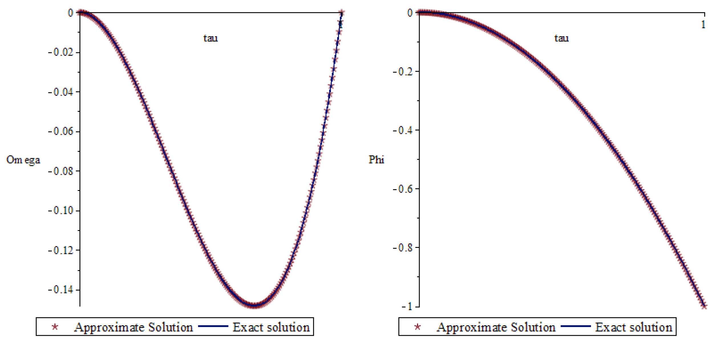
We study the fractional integro-differential system (1) in this example, which has the exact solution as follows:
In this case, we obtain
and
To show the efficiency of this example, we shall offer some numerical testes. For example, for , unknowns are as follows:
Approximate solution is given by
In addition,
Approximate solution is provided by
Table 1 shows the numerical findings obtained for Example 1 using the method we suggest.
Figure 1 depicts the graphs of the achieved absolute errors for Example 1. Here, we note that the symbol in the figures refers to the -axis labels.
Example 2.
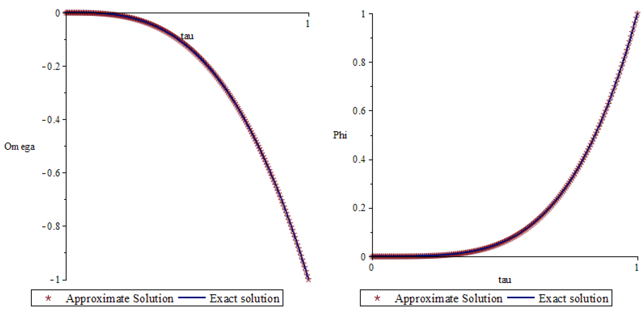
Various types of fractional integro-differential and integral systems can be studied and solved with the proposed method. As a second example for testing, we consider the system of fractional logarithmic integro-differential equations of the following form:
which has the following exact solution:
Here, we have
We provide some numerical tests to demonstrate the efficacy of this illustration. If , then the values of are as shown below:
Approximate solution is given by
In addition,
Approximate solution is provided by
Figure 2 illustrates the numerical results produced for Example 2 using the indicated approach.
Example 3.
Now, we consider the above system of fractional logarithmic integro-differential equations, with the same exact solutions.
In Table 2, we examine the influence of fractional order on the approximate solutions.
7. Conclusions
The application of projection methods is extended in this study so that it can be applied to a fractional Cauchy singular integro-differential system. Shifted Vieta–Lucas polynomials are a class of orthogonal polynomials that serve as the foundation of this approach. The significance of this fractional Cauchy singular integro-differential system is evident in mathematical sciences issues, particularly in physics interactions. It has been observed that the fractional operator has a substantial impact on the development of the numerical results. Numerous kinds of fractional integro-differential and integral systems can be investigated with this method, and their solutions can be found.
Author Contributions
Conceptualization, A.M. (Abdelkader Moumen) and A.M. (Abdelaziz Mennouni); Methodology, A.M. (Abdelkader Moumen) and A.M. (Abdelaziz Mennouni); Investigation, A.M. (Abdelkader Moumen) and A.M. (Abdelaziz Mennouni); Resources, A.M. (Abdelkader Moumen) and A.M. (Abdelaziz Mennouni); Data curation, A.M. (Abdelkader Moumen) and A.M. (Abdelaziz Mennouni); Writing—original draft preparation, A.M. (Abdelkader Moumen) and A.M. (Abdelaziz Mennouni); Writing—review and editing, A.M. (Abdelkader Moumen) and A.M. (Abdelaziz Mennouni); Supervision, A.M. (Abdelkader Moumen) and A.M. (Abdelaziz Mennouni); Funding acquisition, A.M. (Abdelkader Moumen) and A.M. (Abdelaziz Mennouni). All authors have read and agreed to the published version of the manuscript.
Funding
The research of the first author was funded by King Khalid University Researchers Supporting project number RGP.1/350/43, King Khalid University, Abha, Saudi Arabia.
Data Availability Statement
Not applicable.
Acknowledgments
The first author extends his appreciation to the Deanship of Scientific Research at King Khalid University for funding this work through Small Groups (RGP.1/350/43).
Conflicts of Interest
The authors declare no conflict of interest.
References
- Xu, C.; ur Rahman, M.; Baleanu, D. On fractional-order symmetric oscillator with offset-boosting control. Nonlinear Anal. Model. Control. 2022, 27, 994–1008. [Google Scholar] [CrossRef]
- Eskandari, Z.; Avazzadeh, Z.; Khoshsiar Ghaziani, R.; Li, B. Dynamics and bifurcations of a discrete-time Lotka–Volterra model using nonstandard finite difference discretization method. Math Meth. Appl. Sci. 2022. [Google Scholar] [CrossRef]
- Qu, H.D.; Liu, X.; Lu, X.; ur Rahman, M.; She, Z.H. Neural network method for solving nonlinear fractional advection-diffusion equation with spatiotemporal variable-order. Chaos Solitons Fractals 2022, 156, 111856. [Google Scholar] [CrossRef]
- Li, B.; Liang, H.; He, Q. Multiple and generic bifurcation analysis of a discrete Hindmarsh-Rose model. Chaos Solitons Fractals 2021, 146, 110856. [Google Scholar] [CrossRef]
- Li, B.; Liang, H.; Shi, L.; He, Q. Complex dynamics of Kopel model with nonsymmetric response between oligopolists. Chaos Solitons Fractals 2022, 156, 111860. [Google Scholar] [CrossRef]
- Mennouni, A. Two projection methods for skew-hermitian operator equations. Math. Comput. Model. 2012, 55, 1649–1654. [Google Scholar] [CrossRef]
- Araour, M.; Mennouni, A. A New Procedures for Solving Two Classes of Fuzzy Singular Integro-Differential Equations: Airfoil Collocation Methods. Int. J. Appl. Comput. Math. 2022, 8, 35. [Google Scholar] [CrossRef]
- Mennouni, A. A projection method for solving Cauchy singular integro-differential equations. Appl. Math. Lett. 2012, 25, 986–989. [Google Scholar] [CrossRef] [Green Version]
- Mennouni, A. Airfoil polynomials for solving integro-differential equations with logarithmic kernel. Appl. Math. Comput. 2012, 218, 11947–11951. [Google Scholar] [CrossRef]
- Tasci, D.; Yalcin, F. Vieta-Pell and Vieta-Pell-Lucas polynomials. Adv. Differ. Equ. 2013, 2013, 224. [Google Scholar] [CrossRef]
- Izadi, M.; Yüzbaşı, Ş.; Ansari, K.J. Application of Vieta–Lucas Series to Solve a Class of Multi-Pantograph Delay Differential Equations with Singularity. Symmetry 2021, 13, 2370. [Google Scholar] [CrossRef]
- Heydari, M.H.; Avazzadeh, Z.; Razzaghi, M. Vieta-Lucas polynomials for the coupled nonlinear variable-order fractional Ginzburg-Landau equations. Appl. Numer. Math. 2021, 165, 442–458. [Google Scholar] [CrossRef]
- Adel, M.; Assiri, T.A.; Khader, M.M.; Osman, M.S. Numerical simulation by using the spectral collocation optimization method associated with Vieta-Lucas polynomials for a fractional model of non-Newtonian fluid. Results Phys. 2022, 41, 105927. [Google Scholar] [CrossRef]
- Agarwal, P.; El-Sayed, A.A. Vieta–Lucas polynomials for solving a fractional-order mathematical physics model. Adv. Differ. Equ. 2020, 626, 2020. [Google Scholar] [CrossRef]
- Althubiti, S.; Mennouni, A. A Novel Projection Method for Cauchy-Type Systems of Singular Integro-Differential Equations. Mathematics 2022, 10, 2694. [Google Scholar] [CrossRef]
- Mennouni, A. A new efficient strategy for solving the system of Cauchy integral equations via two projection methods. Transylv. J. Math. Mech. 2022, 14, 63–71. [Google Scholar]
Figure 1.
Comparison of exact solutions and and approximate solutions and , respectively, for the first example, where .
Figure 1.
Comparison of exact solutions and and approximate solutions and , respectively, for the first example, where .

Figure 2.
Comparison of exact solutions and and approximate solutions and , respectively, for the second example, where .
Figure 2.
Comparison of exact solutions and and approximate solutions and , respectively, for the second example, where .


Table 1.
Numerical results for Example 1.
| n | ||
|---|---|---|
| 3 | 4.1428 × 10 | 1.5520 × 10 |
| 5 | 8.6994 × 10 | 3.5924 × 10 |
| 7 | 9.6542 × 10 | 8.2544 × 10 |
| 13 | 7.2543 × 10 | 7.2547 × 10 |
| 17 | 9.2541 × 10 | 3.8531 × 10 |
Table 2.
Influence of fractional order on the approximate solutions.
| 0.3 | 1.0548 × 10 | 3.1473 × 10 |
| 0.4 | 1.2668 × 10 | 1.0739 × 10 |
| 0.6 | 7.9977 × 10 | 3.2081 × 10 |
| 0.7 | 8.4737 × 10 | 4.7114 × 10 |
| 0.8 | 9.8905 × 10 | 9.2993 × 10 |
| 1.3 | 9.1313 | 9.7317 |
| 1.6 | 8.4393 × 10 | 2.3766 × 10 |
| 2.4 | 5.1952 × 10 | 7.0123 × 10 |
| 3.7 | 4.0924 × 10 | 1.4281 × 10 |
Disclaimer/Publisher’s Note: The statements, opinions and data contained in all publications are solely those of the individual author(s) and contributor(s) and not of MDPI and/or the editor(s). MDPI and/or the editor(s) disclaim responsibility for any injury to people or property resulting from any ideas, methods, instructions or products referred to in the content. |
© 2022 by the authors. Licensee MDPI, Basel, Switzerland. This article is an open access article distributed under the terms and conditions of the Creative Commons Attribution (CC BY) license (https://creativecommons.org/licenses/by/4.0/).
Share and Cite
MDPI and ACS Style
Moumen, A.; Mennouni, A. A New Projection Method for a System of Fractional Cauchy Integro-Differential Equations via Vieta–Lucas Polynomials. Mathematics 2023, 11, 32. https://0-doi-org.brum.beds.ac.uk/10.3390/math11010032
AMA Style
Moumen A, Mennouni A. A New Projection Method for a System of Fractional Cauchy Integro-Differential Equations via Vieta–Lucas Polynomials. Mathematics. 2023; 11(1):32. https://0-doi-org.brum.beds.ac.uk/10.3390/math11010032
Chicago/Turabian StyleMoumen, Abdelkader, and Abdelaziz Mennouni. 2023. "A New Projection Method for a System of Fractional Cauchy Integro-Differential Equations via Vieta–Lucas Polynomials" Mathematics 11, no. 1: 32. https://0-doi-org.brum.beds.ac.uk/10.3390/math11010032
Note that from the first issue of 2016, this journal uses article numbers instead of page numbers. See further details here.