A New Mathematical Model of COVID-19 with Quarantine and Vaccination

Abstract

A mathematical model revealing the transmission mechanism of COVID-19 is produced and theoretically examined, which has helped us address the disease dynamics and treatment measures, such as vaccination for susceptible patients. The mathematical model containing the whole population was partitioned into six different compartments, represented by the SVEIQR model. Important properties of the model, such as the nonnegativity of solutions and their boundedness, are established. Furthermore, we calculated the basic reproduction number, which is an important parameter in infection models. The disease-free equilibrium solution of the model was determined to be locally and globally asymptotically stable. When the basic reproduction number $R_0$ is less than one, the disease-free equilibrium point is locally asymptotically stable. To discover the approximative solution to the model, a general numerical approach based on the Haar collocation technique was developed. Using some real data, the sensitivity analysis of $R_0$ was shown. We simulated the approximate results for various values of the quarantine and vaccination populations using Matlab to show the transmission dynamics of the Coronavirus-19 disease through graphs. The validation of the results by the Simulink software and numerical methods shows that our model and adopted methodology are appropriate and accurate and could be used for further predictions for COVID-19.

1. Introduction

There is a serious threat to humanity from the coronavirus pandemic and its emerging subtypes. The fast transmission of infections over a short period of time has been enhanced by globalization. This has an impact on the public health care system and restricts the growth of the economies of developing countries. According to studies, COVID-19 has caused more than 92 million recorded infections and 2 million fatalities globally since the outbreak of the pandemic began [1]. To reduce the spread of disease, policymakers continue to use pharmaceutical and non-pharmaceutical interventions such vaccination, isolation of diseased individuals, self-quarantine, face mask use, and travel limitations.

The main symptoms of COVID-19, which appear 14 days after the infection, include coughing, shortness of breath, and fever, according to the Centers for Diseases Control (CDC) [2]. According to the World Health Organization (WHO), coughing or sneezing of possibly infected individuals who are sufficiently close or in contact might create respiratory droplets that can spread COVID-19. High temperatures and high humidity are probably conducive to a decrease in the COVID-19 transmission rate [2]. Up to 24 February 2020, COVID-19 had been the cause of more than 2600 fatalities and 77,000 cases of infection in China alone. On 11 March 2020, WHO identified SARS-CoV-2 as a worldwide pandemic disease [3]. As of 20 April 2020, COVID-19 has caused more than 152,809 human fatalities and 2,246,291 infections, which have been confirmed worldwide, with the USA being the country with the highest number of infections and deaths at 41,000 [2].

Various mathematical models have been proposed by researchers to evaluate the dynamical behavior and transmission of Coronavirus, which may aid in the prediction of future events and even the control of the disease [4,5,6,7,8]. The reproduction number plays a vital role in characterizing the nonlinear dynamics of biological and physical challenges in the study of coronavirus mathematical models. The reproduction rate shows that COVID-19 has either been controlled or has been increasing over time. This study’s objective is to build a modified SIR mathematical model for the prediction of the COVID-19 epidemic’s dynamics taking into consideration several intervention scenarios that might give insight into the best way to proceed to reduce the probability of spread [9,10,11].

We used the Haar wavelets numerical approach for the approximate solution of the model. The simplicity and low computation costs of the Haar approach are its advantages; the suggested technique requires less CPU time and offers more accurate results. For the numerical solution of many differential equations, Chen and Hsia mostly used the technique in the literature [12]. The numerical solution of the integral equations [13] and differential equations [14] was carried out using the Haar wavelet collocation method (HWCT). The pioneering work of Lepik in the development of the HWCT can be seen in [15,16,17,18]. In [19], the authors studied the Euler–Bernoulli nanobeam’s free vibration analysis. For the solution of the initial and boundary value issues, the HWCT is more appropriate. This method provides decent accuracy with fewer collocation points. It is relatively possible to find singularities in irregular structures using the HWCT.

2. Mathematical Model

The goal of this article is to construct a new model of COVID-19 and incorporate the quarantine and vaccination population. The model simulates the dynamics of viral contact, the infection of those who come into contact with the virus, and the absence of the virus after vaccination in those who have not been exposed to the virus.

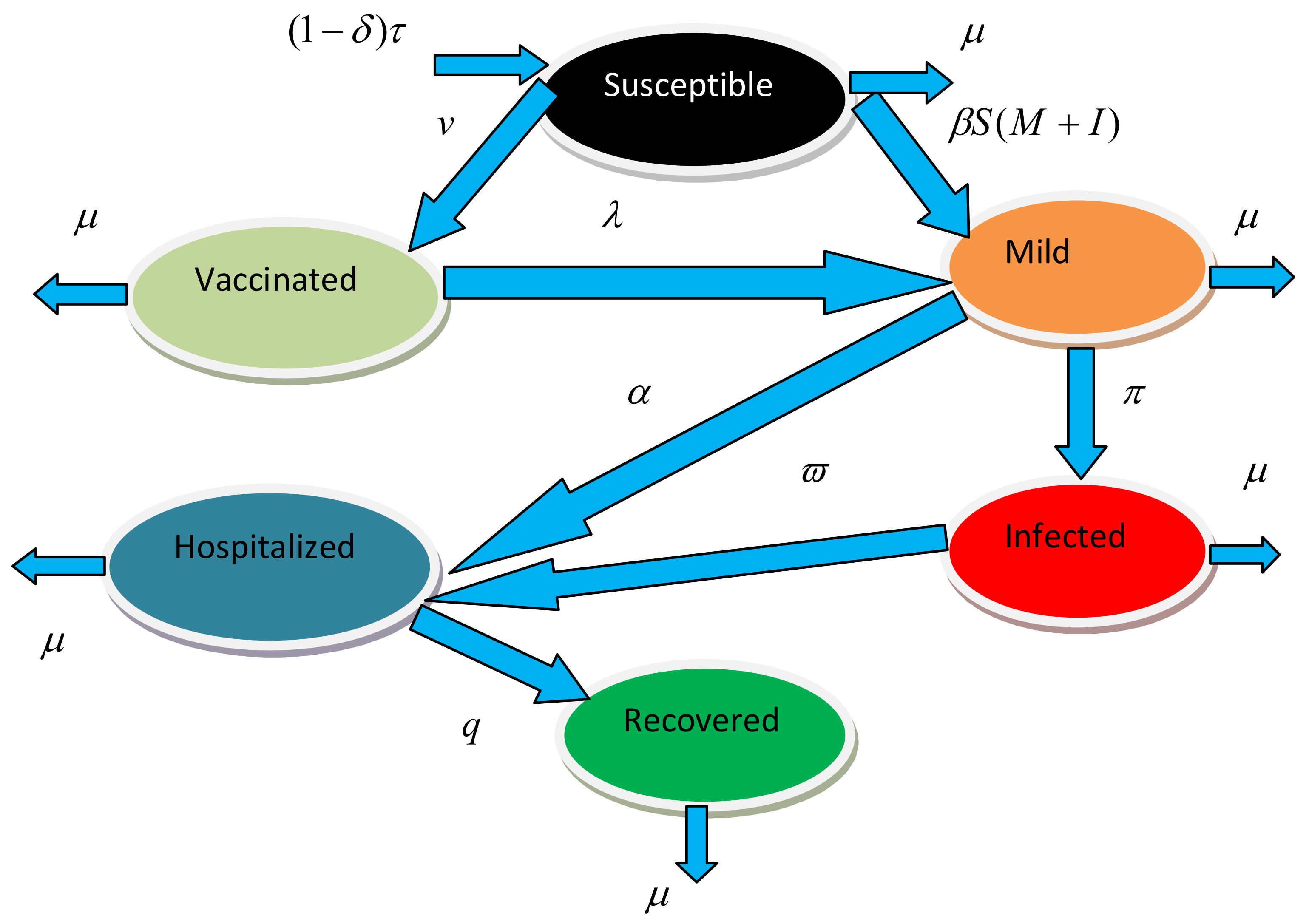
The transmission dynamics of Model (1) are represented in the Figure 1 flowchart.

$$\left\{\begin{array}{cc}\frac{d\mathit{S}}{dt}=\hfill & (1-\delta )\tau -(\mu +v)S-\beta S(E+I),\hfill \\ \frac{d\mathit{V}}{dt}=\hfill & \delta \tau +vS-(\lambda +\mu )V,\hfill \\ \frac{dE}{dt}=\hfill & \beta S(E+I)+\lambda V-(\mu +\alpha +\pi )E,\hfill \\ \frac{dI}{dt}=\hfill & \pi E-(\varpi +\mu )I,\hfill \\ \frac{dQ}{dt}=\hfill & \alpha E+\varpi I-(q+\mu )Q,\hfill \\ \frac{dR}{dt}=\hfill & qQ-\mu R,\hfill \end{array}\right.$$

(1)

with the following initial conditions: $S\left(0\right)>0,V\left(0\right)\ge 0$, $E\left(0\right)\ge 0$, $I\left(0\right)\ge 0$, $Q\left(0\right)\ge 0$, $R\left(0\right)\ge 0$.

Biological Assumptions of the Model

The biological assumptions of the model are as follow:

• We assume that individuals to be vaccinated are selected from individuals who have not been exposed to or immunized against the virus.
• The vaccination may not provide full protection for every person in the vaccine class. In this instance, we suppose that vaccinated people get the virus when they are exposed to it.

The pandemic disease COVID-19 is still active today. On the other hand, several vaccines have been created and are being utilized today to stop epidemic diseases across the globe. There are many mathematical models connected to COVID-19 that do not include vaccinations, but there is almost no research that has taken the vaccine parameter into consideration. In this work, the model SVEIQR comprises the following compartments: susceptible class (S), vaccinated class (V), exposed class (E), infected class (I), quarantine class (Q), and recovered class (R).

In the model, the transition from all ($\tau$) individuals sensitive to the disease is provided. The rate $\beta$ is equal to $\gamma N$. The transition of susceptible people from those who have been exposed to the disease at a rate of $\gamma$, exposed, and those who have not been exposed to it at a rate of v are passed on to those who are vaccinated. Taking into account the possibility that the vaccine developed to fight the COVID-19 virus may be successful or unsuccessful, in the situation that the vaccine is ineffective, as many people as the $\lambda$ ratio to the disease may be exposed. q represents the recovered rate of the quarantine population, and $\mu$ describes the natural death rate.

First, we used fixed point theory to investigate the existence of the newly constructed model (1). On the other hand, stability is important; thus, we discuss the stability of the considered model. We tried to address local and global stability and its many types for the system under consideration by using nonlinear functional analysis to address this objective. Since it is often difficult to find an exact solution to nonlinear problems, to handle such a situation, many numerical methods have been developed in [20,21,22]. Therefore, the results were simulated using Matlab-16 by using the well-known Haar collocation technique. Numerous articles [23,24,25] have made use of the relevant Haar approaches. The COVID-19 mathematical models are very rarely solved by using the Haar collocation methods. We simulated the results using the previously mentioned numerical technique. Finally, the results are shown in comparison to actual data obtained from a source [26].

3. Basic Definitions

Definition 1.

Scaling the function on $\left[{\omega }_1,{\omega }_2\right]$, the Haar wavelet in the Haar family is defined as

$$\begin{array}{ccc}\hfill h_i\left(t\right)& =& \left\{\begin{array}{cc}1\hfill & \mathit{for}t\in \left[\left.{\zeta }_1,{\zeta }_2\right)\right.\hfill \\ -1\hfill & \mathit{for}t\in \left.\left[{\zeta }_2,{\zeta }_3\right.\right)\hfill \\ 0\hfill & \mathit{elsewhere},\hfill \end{array}\right.\hfill \end{array}$$

$h_1\left(t\right)$ and $h_2\left(t\right)$ are called the father and mother wavelets in the Haar wavelet family and are given by

$$\begin{array}{ccc}\hfill h_1\left(t\right)& =& \left\{\begin{array}{cc}1\hfill & \mathit{for}t\in \left[\left.{\omega }_1,{\omega }_2\right)\right.\hfill \\ 0\hfill & \mathit{elsewhere}\hfill \end{array}\right.\hfill \end{array}$$

$$\begin{array}{ccc}\hfill h_2\left(t\right)& =& \left\{\begin{array}{cc}1\hfill & \mathit{for}t\in \left[\left.{\omega }_1,\frac{{\omega }_1+{\omega }_2}{2}\right)\right.\hfill \\ -1\hfill & \mathit{for}t\in \left[\left.\frac{{\omega }_1+{\omega }_2}{2},{\omega }_2\right)\right.\hfill \\ 0\hfill & \mathit{elsewhere}.\hfill \end{array}\right.\hfill \end{array}$$

where ${\zeta }_1={\omega }_1+({\omega }_2-{\omega }_1)\frac{\zeta }{d},$${\zeta }_2={\omega }_1+({\omega }_2-{\omega }_1)\frac{\zeta +0.5}{d},$${\zeta }_3={\omega }_1+({\omega }_2-{\omega }_1)\frac{\zeta +1}{d}$, where $d=2^r$ and $\zeta =0,1,\dots ,d-1.$ If we take interval $[0,1]$, then the values of ${\zeta }_1,{\zeta }_2,{\zeta }_3,$ are: ${\zeta }_1=\frac{\zeta }{d},$${\zeta }_2=\frac{1/2+\zeta }{d},{\zeta }_3=\frac{1+\zeta }{d}.$ We truncated this series at M terms, $u\left(t\right)={\sum }_{k=1}^M{\lambda }_k{h}_k\left(t\right).$ The role of integer i is to count the functions in the HW family, and it satisfies the relation $i=1+\zeta +d$.

We introduce the following notations for integrals of Haar functions:

$$\begin{array}{ccc}\hfill p_{i,1}\left(t\right)& =& \underset{0}{\overset{t}{\int }}{h}_i\left(s\right)ds\hfill \end{array}$$

and

$$\begin{array}{ccc}\hfill p_{i,1}\left(t\right)& =& \left\{\begin{array}{cc}t-{\zeta }_1\mathrm{if}\hfill & t\in ({\zeta }_1,{\zeta }_2),\hfill \\ {\zeta }_3-t\mathrm{if}\hfill & t\in ({\zeta }_2,{\zeta }_3)\hfill \\ 0\hfill & \mathrm{other}\mathrm{where}\hfill \end{array}\right.\hfill \end{array}$$

Generally,

$$\begin{array}{ccc}\hfill p_{i,n}\left(t\right)& =& \underset{0}{\overset{t}{\int }}{p}_{i,n-1}\left(x\right)dx\hfill \end{array}$$

Thus,

$$\begin{array}{ccc}\hfill p_{i,n}\left(t\right)& =& \left\{\begin{array}{cc}0\hfill & \mathrm{if}t\in \left[\left.0,{\zeta }_1\right)\right.,\hfill \\ \frac{{(t-{\zeta }_1)}^n}{n!}\hfill & \mathrm{if}t\in \left[\left.{\zeta }_1,{\zeta }_2\right)\right.\hfill \\ \frac{{(t-{\zeta }_1)}^n-2{({\zeta }_1-{\zeta }_2)}^n}{n!}\hfill & \mathrm{if}t\in \left[\left.{\zeta }_2,{\zeta }_3\right)\right.\hfill \\ \frac{1}{n!}{[t-{\zeta }_1)}^n-2{({\zeta }_1-{\zeta }_2)}^n+{(t-{\zeta }_3)}^n]\hfill & \mathrm{if}t\in \left[\left.{\zeta }_3,1\right)\right..\hfill \end{array}\right.\hfill \end{array}$$

Definition 2.

The interval $\left[{\gamma }_1,{\gamma }_2\right]$ for the HWCT is discretized as

$$\begin{array}{c}\hfill \begin{array}{cc}\hfill t_1={\gamma }_1+({\gamma }_2-{\gamma }_1)\frac{i-1/2}{2M},& i=1,2,\dots \dots ,2M.\hfill \end{array}\end{array}$$

The collocation points are defined in the above equation.

Remark 1.

The integral in the above equation can be calculated by the following formula:

$$\begin{array}{ccc}\hfill \underset{{\gamma }_1}{\overset{{\gamma }_2}{\int }}u\left(x\right)dx& \approx & \frac{{\gamma }_2-{\gamma }_1}{M}\sum _{i=1}^{M}u\left(x_i\right)=\frac{{\gamma }_2-{\gamma }_1}{M}\sum _{i=1}^{M}u({\gamma }_1+({\gamma }_2-{\gamma }_1)\frac{(i-0.5)}{n}).\hfill \end{array}$$

4. Mathematical Analysis of System (1)

Positivity and Boundedness of the Solutions

In this section, we prove the positivity and boundedness of the solution of the model (1)

$$\begin{array}{c}\hfill \begin{array}{cc}& {\left.\frac{dS}{dt}\right|}_{S=0}=(1-\delta )\tau ,{\left.\frac{dV}{dt}\right|}_{V=0}=\delta \tau ,\hfill \\ & {\left.\frac{dE}{dt}\right|}_{E=0}=\beta SI+\alpha V,{\left.\frac{dI}{dt}\right|}_{I=0}=\pi E\left(t\right),\hfill \\ & {\left.\frac{dQ}{dt}\right|}_{Q=0}=\alpha E+\varpi I,{\left.\frac{dR}{dt}\right|}_{R=0}=qQ.\hfill \end{array}\end{array}$$

On the bounding planes, each rate is nonnegative in this case. If we begin in the interior of the six-dimensional closed hyper octant ${\mathcal{R}}^6$, we will always remain there.

Additionally, we see from System (1) that the entire human population N satisfies

$$\frac{dN}{dt}=\frac{dS}{dt}+\frac{dV}{dt}+\frac{dE}{dt}+\frac{dI}{dt}+\frac{dQ}{dt}+\frac{dR}{dt}.$$

(2)

Then, putting Equation (1) in Equation (2) gives

$$\begin{array}{cc}\hfill \frac{dN}{dt}=& \left[(1-\delta )\tau -(\mu +v)S-\beta S(E+I)\right]\hfill \\ \hfill & +\left[\delta \tau +vS-(\lambda +\mu )V\right]+\left[\beta S(E+I)\right.\hfill \\ \hfill & \left.+\lambda V-(u+\alpha +\pi )E\right]+\left[\pi E-\varpi I-uI\right]\hfill \\ \hfill & +\left[\alpha E+\varpi I-(q+u)Q\right]+\left[qQ-uR\right].\hfill \end{array}$$

(3)

Simplifying Equation (3), we obtain

$$\frac{dN}{dt}=\tau -\mu \left(S+V+E+I+Q+R\right)$$

(4)

Applying Equation (2) and Equation (4), we obtain

$$\frac{dN}{dt}=\tau -\mu N,$$

(5)

$$\frac{dN}{dt}+\mu N=\tau .$$

(6)

Solving Equation (6) and using the initial conditions, we conclude that all solutions in Equation (1) belong to the region $\Omega =\left\{\left(S,V,E,I,Q,R\right)\in {\mathbb{R}}_{+}^6:0\le N\le \frac{\tau }{\mu }\right\}$ for $\left(S\right(0),V(0),E(0),I(0),Q(0),R(0\left)\right)\in \Omega .$

5. Equilibrium Points of the Model

The disease-free equilibrium point ${\mathcal{E}}^0$ can be found by making the right side of System (1) equal to zero and solving for the variables, which gives ${\mathcal{E}}^0$ as

$${\mathcal{E}}^0=\left(S^0,V^0,E^0,I^0,Q^0,R^0\right)=\left(\frac{(1-\delta )\tau }{(\mu +v)},\frac{(\mu +v)\delta \tau +(1-\delta )v\tau }{(\lambda +\mu )(\mu +v)},0,0,0,0\right).$$

(7)

5.1. Basic Reproduction Number $\left({\mathcal{R}}_0\right)$

$\left({\mathcal{R}}_0\right)$ is the estimated number of secondary cases by a single infection in a total susceptible population. The expression of the basic reproduction number ${\mathcal{R}}_0$, widely utilized by public health organizations as a fundamental indicator of the severity of a particular epidemic, is found using the next-generation matrix approach [26]. The system’s new infection and transition terms are provided, respectively, by

$$\mathcal{F}=\left(\begin{array}{c}\beta S(E+I)\\ 0\\ 0\end{array}\right).$$

(8)

$$\mathcal{U}=\left(\begin{array}{c}-\lambda V+(u+\alpha +\pi )E\\ -\pi E+(\varpi +u)I\\ -\alpha E-\varpi I+(q+u)Q\end{array}\right).$$

(9)

The matrices U (of transition terms) and F (of new infection terms) are now determined to be

$$F=\left(\begin{array}{ccc}\frac{\gamma (1-\delta ){\tau }^2}{\mu (\mu +v)}& \frac{(1-\delta )\gamma {\tau }^2}{\mu (\mu +v)}& 0\\ 0& 0& 0\\ 0& 0& 0\end{array}\right).$$

(10)

$$U=\left(\begin{array}{ccc}u+\alpha +\pi & 0& 0\\ -\pi & \varpi +u& 0\\ -\alpha & -\varpi & q+u\end{array}\right).$$

(11)

It follows that

$$U^{-1}=\left(\begin{array}{ccc}\frac{1}{u+\alpha +\pi }& 0& 0\\ \frac{\pi }{(u+\alpha +\pi )\varpi +u}& \frac{1}{\varpi +u}& 0\\ \frac{\pi \varpi +\varpi \alpha +\alpha u}{(u+\alpha +\pi )(\varpi +u)(q+u)}& \frac{\varpi }{(\varpi +u)(q+u)}& \frac{1}{q+u}\end{array}\right).$$

(12)

It follows that

$$F{U}^{-1}=\left(\begin{array}{ccc}\frac{\gamma (1-\delta ){\tau }^2}{\mu (\mu +v)(u+\alpha +\pi )}+\frac{\pi (1-\delta )\gamma {\tau }^2}{\mu (\mu +v)\left(\right(u+\alpha +\pi )\varpi +u)}& \frac{(1-\delta )\gamma {\tau }^2}{\mu (\varpi +u)(\mu +v)}& 0\\ 0& 0& 0\\ 0& 0& 0\end{array}\right).$$

(13)

Since ${\mathcal{R}}_0$ is the dominant eigenvalue of the next-generation matrix $F{U}^{-1}$, the largest eigenvalue of $F{U}^{-1}$ is

$${\mathcal{R}}_0=\frac{\gamma (1-\delta ){\tau }^2}{\mu (\mu +v)(u+\alpha +\pi )}+\frac{\pi (1-\delta )\gamma {\tau }^2}{\mu (\mu +v)(u+\alpha +\pi )(\varpi +u)}.$$

(14)

It is clear from the equation of the fundamental reproduction number that the value of ${\mathcal{R}}_0$ decreases with an increase in the vaccination and quarantine rates.

Theorem 1.

The disease-free equilibrium point ${\mathcal{E}}^0$ is locally stable when ${\mathcal{R}}_0<1$.

Proof. 

For local stability at ${\mathcal{E}}^0$, the Jacobian matrix of System (1) is

$${\mathcal{J}}_{{\mathcal{E}}^0}=\left(\begin{array}{cccccc}-(\mu +v)& 0& -\frac{\beta (1-\delta )\tau }{(\mu +v)}& -\frac{\beta (1-\delta )\tau }{(\mu +v)}& 0& 0\\ v& -(\lambda +\mu )& 0& 0& 0& 0\\ 0& \lambda & \frac{\beta (1-\delta )\tau }{(\mu +v)}-(u+\alpha +\pi )& \frac{\beta (1-\delta )\tau }{(\mu +v)}& 0& 0\\ 0& 0& \pi & -(\varpi +u)& 0& 0\\ 0& 0& \alpha & \varpi & -(q+u)& 0\\ 0& 0& 0& 0& q& -u\end{array}\right),$$

(15)

which follows the eigenvalues, ${\lambda }_1<0$, ${\lambda }_2<0$, ${\lambda }_3<0$, ${\lambda }_4<0$, ${\lambda }_5<0$, and ${\lambda }_6<0,$ if ${\mathcal{R}}_0<1$. Therefore, System (1) is locally stable if ${\mathcal{R}}_0<1$ and unstable if ${\mathcal{R}}_0>1.$ □

5.2. Global Stability of Disease-Free Equilibrium Point

We now study the global stability of the DFE using the approach described in [27]. Consider a system of ordinary differential equations of the form

$$\left\{\begin{array}{cc}\frac{dx}{dt}=\hfill & \mathcal{F}\left(x,I\right),\hfill \\ \frac{dI}{dt}=\hfill & \mathcal{G}\left(x,I\right),\left(x,0\right)=0,\hfill \end{array}\right.$$

(16)

where $x\in {\mathbb{R}}^n$ denotes (its components) the number of uninfected individuals and $I\in {\mathbb{R}}^m$ denotes (its components) the number of infected individuals, including latent and infectious. Let ${\mathcal{U}}_0=\left(x^{*},0\right)$ be the disease-free equilibrium of this system, where 0 is a zero vector. The global stability of the DFE is guaranteed when the following conditions ($H_1$) and ($H_2$) are satisfied.

• $\left(H_1\right)$ For $\frac{dx}{dt}=\mathcal{F}\left(x,0\right),0$ is globally asymptotically stable.
• $\left(H_2\right)$$\overline{\mathcal{G}}\left(x,I\right)=BI-\mathcal{G}\left(x,I\right),\overline{\mathcal{G}}\left(x,I\right)\ge 0,$ for $\left(x,I\right)\in \Delta ,$ where $B=D_1\mathcal{G}\left(x^{*},0\right)$ is an M-matrix (the off-diagonal elements of B are nonnegative), and $\Delta$ is the region where the model makes biological sense.

Corollary 1

(see [27]). The fixed point ${\mathcal{U}}_0\left(x^{*},0\right)$ is a globally asymptotic stable (g.a.s.) equilibrium of (16) provided that ${\mathcal{R}}_0<1$ (l.a.s.) and that assumptions ($H_1$) and ($H_2$) are satisfied.

Theorem 2.

The DFE ${\mathcal{E}}_0$ of Model (1) is globally asymptotically stable if ${\mathcal{R}}_0<1$.

Proof. 

First, we rewrite Model (1) by setting $x=\left(S,V\right)$ and $I=\left(E,I,Q,R\right)$.

Then, the DFE is given by

${\mathcal{U}}_0=\left(x^{*},0\right)=\left(\frac{(1-\delta )\lambda \left(({\mathcal{R}}_0-1)\delta {\tau }^2\gamma (1-\delta )\tau (\varpi +u+\pi )+(u+\alpha +\pi )(\varpi +u)\right)}{(\mu +v)+\gamma (\lambda +\mu )(\varpi +u+\pi )},\frac{\delta \tau }{(\lambda +\mu )}+\frac{v(1-\delta )\lambda \left(({\mathcal{R}}_0-1)\delta \tau \gamma (1-\delta )\tau (\varpi +u+\pi )(u+\alpha +\pi )(\varpi +u)\right)}{(\mu +v)+\gamma (\varpi +u+\pi )},0\right)$ and the system $\frac{dx}{dt}=\mathcal{F}\left(x,0\right)$ becomes

$$\left\{\begin{array}{cc}\dot{S}=\hfill & (1-\delta )\tau -(\mu +v)S\hfill \\ \dot{V}=\hfill & \delta \tau +vS-\mu V.\hfill \end{array}\right.$$

(17)

This equation has a unique equilibrium point:

$$x^{*}=\left(\frac{(1-\delta )\tau }{(\mu +v)},\frac{v(1-\delta )\tau +\delta \tau (\mu +v)}{\mu (\mu +v)}\right)$$

(18)

which is globally asymptotically stable. Therefore, the condition ($H_1$) is satisfied.

We now verify the second condition ($H_2$). For Model (1), we have

$$\mathcal{G}\left(x,I\right)=\left(\begin{array}{c}\beta S(E+I)+\lambda V-(u+\alpha +\pi )E\\ \pi E-(\varpi +u)I\\ \alpha E+\varpi I-(q+u)Q\\ qQ-uR\end{array}\right).$$

(19)

$$D_1\mathcal{G}\left(x^{*},0\right)=\left(\begin{array}{cccc}\beta S^0& \beta S^0& 0& 0\\ \pi & -(\varpi +u)& 0& 0\\ \alpha & \varpi & -(q+u)& 0\\ 0& 0& q& -u\end{array}\right).$$

(20)

Clearly, B is an M-matrix. On the other hand,

$$\begin{array}{ccc}\hfill \overline{\mathcal{G}}\left(x,I\right)=BI-\mathcal{G}\left(x,I\right)& =& \left(\begin{array}{c}\left(\frac{\beta (1-\delta )\tau }{(\mu +v)}\right)\frac{(\mu +v)\delta \tau +(1-\delta )v\tau }{(\lambda +\mu )(\mu +v)}\\ 0\\ 0\\ 0\end{array}\right)\hfill \end{array}$$

which implies that $\overline{\mathcal{G}}\left(x,I\right)\ge 0$, for all $\left(x,I\right)\in \Delta$. Therefore, the conditions ($H_1$) and ($H_2$) are satisfied. By Corollary 1, the global stability of the DFE is obtained. This completes the proof. □

5.3. Stability of $E^{*}$

The stability of the endemic steady state $E^{*}$ is present in this subsection.

Theorem 3.

There exists a unique positive virus equilibrium point ${\mathcal{E}}^{*}=\left(S^{*},V^{*},E^{*},I^{*},Q^{*},R^{*}\right)$ for System (1), if ${\mathcal{R}}_0>1.$

Proof. 

By letting the right-hand sides of all equations of System (1) be zero, as

$$\begin{array}{cc}& (1-\delta )\tau -(\mu +v)S-\beta S(E+I)=0,\hfill \\ \hfill & \delta \tau +vS-(\lambda +\mu )V=0,\hfill \\ \hfill & \beta S(E+I)+\lambda V-(u+\alpha +\pi )E=0,\hfill \\ \hfill & \pi E-(\varpi +u)I=0,\hfill \\ \hfill & \alpha E+\varpi I-(q+u)Q=0,\hfill \\ \hfill & qQ-uR=0.\hfill \end{array}$$

(21)

which implies that the endemic steady state as ${\mathcal{E}}^{*}=\left(S^{*},V^{*},E^{*},I^{*},Q^{*},R^{*}\right),$ where

$$\begin{array}{cc}& S^{*}=\frac{(1-\delta )\lambda \left(({\mathcal{R}}_0-1)\delta {\tau }^2\gamma (1-\delta )\tau (\varpi +u+\pi )+(u+\alpha +\pi )(\varpi +u)\right)}{(\mu +v)+\gamma (\lambda +\mu )(\varpi +u+\pi )},\end{array}$$

$$\begin{array}{cc}& E^{*}=\frac{(\varpi +u)\lambda \left(({\mathcal{R}}_0-1)\delta \tau \pi \gamma (1-\delta )\tau (\varpi +u+\pi )+(u+\alpha +\pi )(\varpi +u)\right)}{\pi (\lambda +\mu )},\end{array}$$

$$\begin{array}{cc}& V^{*}=\frac{\delta \tau }{(\lambda +\mu )}+\frac{v(1-\delta )\lambda \left(({\mathcal{R}}_0-1)\delta \tau \gamma (1-\delta )\tau (\varpi +u+\pi )(u+\alpha +\pi )(\varpi +u)\right)}{(\mu +v)+\gamma (\varpi +u+\pi )},\end{array}$$

$$\begin{array}{cc}& I^{*}=\frac{\lambda \left(({\mathcal{R}}_0-1)\delta \tau \pi \gamma (1-\delta )\tau (\varpi +u+\pi )+(u+\alpha +\pi )(\varpi +u)\right)}{(\lambda +\mu )},\end{array}$$

$$\begin{array}{cc}& Q^{*}=\frac{\alpha (\varpi +u)+\varpi \pi (\lambda +\mu )}{(q+u)\lambda \left({\mathcal{R}}_0-1)\delta {\tau }^2{\pi }^2\gamma (1-\delta )(\varpi +u+\pi )+(u+\alpha +\pi )(\varpi +u)\right)},\end{array}$$

$$\begin{array}{cc}& R^{*}=\frac{\left(q\alpha (\varpi +u)+q\varpi \pi \right)\left(\lambda ({\mathcal{R}}_0-1)\delta \tau \pi \gamma (1-\delta )\tau (\varpi +u+\pi )+(u+\alpha +\pi )(\varpi +u)\right)}{\pi u(q+u)(\lambda +\mu )},\end{array}$$

The expression $(1-\delta )$ is positive since $\delta$ refers to the proportion of infectious cases that are asymptomatic, but later develop symptoms; it ranges from 0 and 1. It is clear from the above that, when ${\mathcal{R}}_0>1$, the positive endemic steady state of System (1) only exists. System (1) thus has an endemic equilibrium state whenever ${\mathcal{R}}_0>1$ and possesses no endemic state when ${\mathcal{R}}_0\le 1$. □

6. Sensitivity Analysis

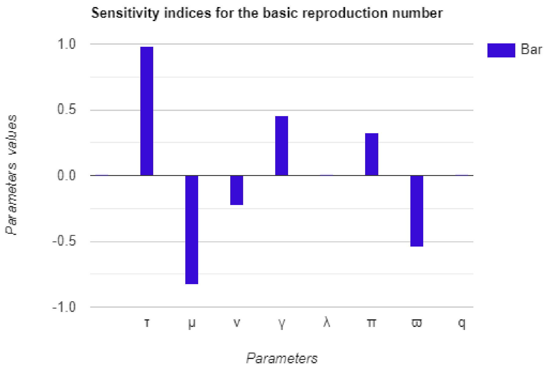
We present the sensitivity analysis in this part to compensate the factors that have a significant influence on the basic reproduction number. Sensitivity analysis is suggested to comprehend the relative significance of the many factors responsible for disease transmission and prevalence. It is essential to regulate the variations in the SVEIQR model parameters to produce ${\mathcal{R}}_0<1$ in order to control the spread of diseases. The ratio of the change in a variable to the change in a parameter is known as the sensitivity index, and it can be calculated using the formula $S\left[x\right]=\frac{x}{{\mathcal{R}}_0}\times \frac{\partial {\mathcal{R}}_0}{\partial x}$.

Table 1. Sensitivity indices of ${\mathcal{R}}_0$ with respect to model parameters.

Parameters	Parameters Sensitivity Index
$S\left[\tau \right]$	=$\frac{\tau }{{\mathcal{R}}_0}\times \frac{\partial {\mathcal{R}}_0}{\partial \tau }=0.983>0,$
$S\left[\mu \right]$	=$\frac{\mu }{{\mathcal{R}}_0}\times \frac{\partial {\mathcal{R}}_0}{\partial \mu }=-0.832<0$
$S\left[\nu \right]$	=$\frac{\nu }{{\mathcal{R}}_0}\times \frac{\partial {\mathcal{R}}_0}{\partial \nu }=-0.23<0$
$S\left[\gamma \right]$	=$\frac{\gamma }{{\mathcal{R}}_0}\times \frac{\partial {\mathcal{R}}_0}{\partial \gamma }=0.453>0$
$S\left[\lambda \right]$	=$\frac{\lambda }{{\mathcal{R}}_0}\times \frac{\partial {\mathcal{R}}_0}{\partial \lambda }=0$
$S\left[\pi \right]$	=$\frac{\pi }{{\mathcal{R}}_0}\times \frac{\partial {\mathcal{R}}_0}{\partial \pi }=0.325>0$
$S\left[\varpi \right]$	=$\frac{\varpi }{{\mathcal{R}}_0}\times \frac{\partial {\mathcal{R}}_0}{\partial \varpi }=-0.5421<0$
$S\left[q\right]$	=$\frac{q}{{\mathcal{R}}_0}\times \frac{\partial {\mathcal{R}}_0}{\partial q}$=0

provides the sensitivity indices of ${\mathcal{R}}_0<1$ with regard to the model parameters.

It is clear from Table 1 and Figure 2 that the most sensitive parameter to ${\mathcal{R}}_0$ for the SVEIQR model is the disease transmission rate, infectious rate $\gamma$, quarantine rate of the infected people $\varpi$, and vaccination rate v. The value of ${\mathcal{R}}_0$ increases when the value of $\gamma$ increases. The value of ${\mathcal{R}}_0$ decreases when the vaccination (v) and quarantine rates of the infected people ($\varpi$) increase. Thus, ${\mathcal{R}}_0$ increases with the decreases of the vaccination (v) and quarantine rate ($\varpi$).

Clearly, Figure 2 describes that the value of ${\mathcal{R}}_0$ increases with the increases in the values of parameters $\gamma ,\pi$ and $\tau$ as these parameters possess positive indices with ${\mathcal{R}}_0$. Similarly, the parameters having negative indices with ${\mathcal{R}}_0$ are $\alpha ,\varpi$ and v. As a result, increases in these parameters result in a decrease in the value of ${\mathcal{R}}_0$. It is obvious that the presence of a lower value of ${\mathcal{R}}_0$ contributes to the decrease in disease incidence. In order to eradicate the disease from the system, we must reduce the efficacy of parameters with positive indices to a basic reproduction number, while maintaining parameters with negative indices. Therefore, in order to limit future outbreaks, health authorities must give careful consideration to any preventative action that will lessen the disease burden. We discovered that sufficient hygiene and effective health care services should be used to implement the control parameters, such as the use of vaccinations v and quarantine $\varpi$ effectiveness, etc., which are negatively associated with ${\mathcal{R}}_0$.

7. Numerical Scheme for System (1)

The implementation of the Haar approach is discussed in this part in order to determine a solution for the suggested model. Utilizing the Haar function, the derivative of the unknown function in the nonlinear system was approximated, and the equation for the unknown function was determined by integration. We obtained the system of algebraic equations by inserting the nodal points using the collocation method on these equations. In order to identify the unknown coefficients, Broyden’s method was used to solve these nonlinear equations. Finally, utilizing these unknowable coefficients, the approximative solution at nodal points was derived.

Numerical Scheme

Let $\dot{S}$$,\dot{V},\dot{E},\dot{I},\dot{Q},$ and $\dot{R}$ considering that they are in the space of square integrable functions ($L_2[0,1)$). Consequently, the Haar series can be expressed as

$$\begin{array}{c}\hfill \dot{S}\left(t\right)={\displaystyle \sum _{i=1}^M{a}_i{h}_i\left(t\right)},\dot{V}\left(t\right)={\displaystyle \sum _{i=1}^M{b}_i{h}_i\left(t\right),}\\ \hfill \dot{E}\left(t\right)={\displaystyle \sum _{i=1}^M{c}_i{h}_i\left(t\right)},\dot{I}\left(t\right)={\displaystyle \sum _{i=1}^M{d}_i{h}_i\left(t\right),}\\ \hfill \dot{Q}\left(t\right)={\displaystyle \sum _{i=1}^M{e}_i{h}_i\left(t\right)},\dot{R}\left(t\right)={\displaystyle \sum _{i=1}^M{g}_i{h}_i\left(t\right)}.\end{array}$$

(22)

Integration of the above Equation (22) and using the initial condition, we obtain

$$\begin{array}{cc}\hfill S\left(t\right)=S_0+{\displaystyle \sum _{i=1}^M{a}_i{p}_i\left(t\right)},& V\left(t\right)=V_0+{\displaystyle \sum _{i=1}^M{b}_i{p}_i\left(t\right)},\hfill \\ \hfill E\left(t\right)=E_0+{\displaystyle \sum _{i=1}^M{c}_i{p}_i\left(t\right)},& I\left(t\right)=I_0+{\displaystyle \sum _{i=1}^M{d}_i{p}_i\left(t\right)},\hfill \\ \hfill Q\left(t\right)=Q_0+{\displaystyle \sum _{i=1}^M{e}_i{p}_i\left(t\right)},& R\left(t\right)=R_0+{\displaystyle \sum _{i=1}^M{g}_i{p}_i\left(t\right)}.\hfill \end{array}$$

(23)

We have

$$\begin{array}{cc}\hfill \dot{S}\left(t\right)dt=& (1-\delta )\tau -(\mu +v)S-\beta S(E+I)\hfill \\ \hfill \dot{V}\left(t\right)dt=& \delta \tau +vS-(\lambda +\mu )V,\hfill \\ \hfill \dot{E}\left(t\right)dt=& \beta S(E+I)+\lambda V-(u+\alpha +\pi )E,\hfill \\ \hfill \dot{I}\left(t\right)dt=& \pi E-(\varpi +u)I,\hfill \\ \hfill \dot{Q}\left(t\right)dt=& \alpha E+\varpi I-(q+u)Q,\hfill \\ \hfill \dot{R}\left(t\right)dt=& qQ-uR.\hfill \end{array}$$

(24)

Applying Haar approximations to Equation (24), we obtain

$$\begin{array}{cc}\hfill \begin{array}{c}\hfill \sum _{i=1}^M{a}_i{h}_i\left(t\right)dt=\end{array}& (1-\delta )\tau -(\mu +v){\displaystyle \left(S_0+\sum _{i=1}^M{a}_i{p}_i\left(t\right)\right)}-\gamma N\left(S_0+\sum _{i=1}^M{a}_i{p}_i\left(t\right)\right)\hfill \\ \hfill & \left(\left(E_0+{\displaystyle \sum _{i=1}^M{c}_i{p}_i\left(t\right)}\right)+\left(I_0+\sum _{i=1}^M{d}_i{p}_i\left(t\right)\right)\right),\hfill \end{array}$$

$$\begin{array}{c}\hfill \begin{array}{cc}\hfill {\displaystyle \sum _{i=1}^M{b}_i{h}_i\left(t\right)dt}=& \delta \tau +v\left(S_0+\sum _{i=1}^M{a}_i{p}_i\left(t\right)\right)-(\lambda +\mu ){\displaystyle \left(V_0+\sum _{i=1}^M{b}_i{p}_i\left(t\right)\right),}\hfill \end{array}\end{array}$$

$$\begin{array}{cc}\hfill \begin{array}{c}\hfill {\displaystyle \sum _{i=1}^M{c}_i{h}_i\left(t\right)}dt=\end{array}& \beta \left(S_0+\sum _{i=1}^M{a}_i{p}_i\left(t\right)\right)\left(\left(E_0+{\displaystyle \sum _{i=1}^M{c}_i{p}_i\left(t\right)}\right)+\left(I_0+\sum _{i=1}^M{d}_i{p}_i\left(t\right)\right)\right)\hfill \\ \hfill & +\lambda \left(V_0+{\displaystyle \sum _{i=1}^M{b}_i{p}_i\left(t\right)}\right)-(u+\alpha +\pi )\left(E_0+{\displaystyle \sum _{i=1}^M{c}_i{p}_i\left(t\right))}\right),\hfill \end{array}$$

$$\begin{array}{c}\hfill \begin{array}{cc}\hfill {\displaystyle \sum _{i=1}^{M}di{h}_i\left(t\right)}dt=& \pi {\displaystyle \left(E_0+\sum _{i=1}^M{c}_i{p}_i\left(t\right)\right)}-(\varpi +u){\displaystyle \left(I_0+\sum _{i=1}^M{d}_i{p}_i\left(t\right)\right),}\hfill \end{array}\end{array}$$

$$\begin{array}{cc}\hfill \begin{array}{c}\hfill {\displaystyle \sum _{i=1}^M{e}_i{h}_i\left(t\right)}dt=\end{array}& \alpha \left(E_0+{\displaystyle \sum _{i=1}^M{c}_i{p}_i\left(t\right)}\right)+\varpi \left(I_0+\sum _{i=1}^M{d}_i{p}_i\left(t\right)\right)\hfill \\ \hfill & -(q+u){\displaystyle \left(Q_0+\sum _{i=1}^M{g}_i{p}_i\left(t\right)\right)},\hfill \end{array}$$

$$\begin{array}{c}\hfill \begin{array}{cc}\hfill {\displaystyle \sum _{i=1}^M{g}_i{h}_i\left(t\right)}dt=& q{\displaystyle \left(Q_0+\sum _{i=1}^M{e}_i{p}_i\left(t\right)\right)}-u{\displaystyle \left(R_0+\sum _{i=1}^M{g}_i{p}_i\left(t\right)\right).}\hfill \end{array}\end{array}$$

Upon simplification, we have

$$\begin{array}{cc}\hfill & \sum _{i=1}^M{a}_i{h}_i\left(t\right)dt-(1-\delta )\tau +\mu S_0+\nu S_0+\mu \sum _{i=1}^M{a}_i{p}_i\left(t\right)\hfill \\ \hfill & +\nu \sum _{i=1}^M{a}_i{p}_i\left(t\right)+\beta S_0{E}_0+\gamma N{S}_0{I}_0+\beta S_0{\displaystyle \sum _{i=1}^M{c}_i{p}_i\left(t\right)}\hfill \\ \hfill & +{\displaystyle \beta S_0\sum _{i=1}^M{d}_i{p}_i\left(t\right)+\beta E_0{\displaystyle \sum _{i=1}^M{a}_i{p}_i\left(t\right)+\beta I_0{\displaystyle \sum _{i=1}^M{a}_i{p}_i\left(t\right)}}}\hfill \\ \hfill & +\beta {\displaystyle \sum _{i=1}^M{a}_i{p}_i\left(t\right)}{\displaystyle \sum _{i=1}^M{c}_i{p}_i\left(t\right)+\beta {\displaystyle \sum _{i=1}^M{a}_i{p}_i\left(t\right)}{\displaystyle \sum _{i=1}^M{d}_i{p}_i\left(t\right)=0},}\hfill \end{array}$$

(25)

$$\begin{array}{cc}\hfill & {\displaystyle \sum _{i=1}^M{b}_i{h}_i\left(t\right)dt-\delta \tau -\nu S_0}-v\sum _{i=1}^M{a}_i{p}_i\left(t\right)+\lambda V_0\hfill \\ \hfill & +\lambda {\displaystyle \sum _{i=1}^M{b}_i{p}_i\left(t\right)}+\mu V_0+\mu {\displaystyle \sum _{i=1}^M{b}_i{p}_i\left(t\right)=0,}\hfill \end{array}$$

(26)

$$\begin{array}{cc}\hfill & {\displaystyle \sum _{i=1}^M{c}_i{h}_i\left(t\right)}dt-\beta S_0{E}_0-\beta S_0{\displaystyle \sum _{i=1}^M{c}_i{p}_i\left(t\right)}-\beta S_0{I}_0\hfill \\ \hfill & -\beta S_0{\displaystyle \sum _{i=1}^M{d}_i{p}_i\left(t\right)-\beta E_0{\displaystyle \sum _{i=1}^M{a}_i{p}_i\left(t\right)-\beta I_0{\displaystyle \sum _{i=1}^M{a}_i{p}_i\left(t\right)}}}\hfill \\ \hfill & +\beta {\displaystyle \sum _{i=1}^M{a}_i{p}_i\left(t\right)}{\displaystyle \sum _{i=1}^M{c}_i{p}_i\left(t\right)-\beta {\displaystyle \sum _{i=1}^M{a}_i{p}_i\left(t\right)}{\displaystyle \sum _{i=1}^M{d}_i{p}_i\left(t\right)}}\hfill \\ \hfill & -\lambda V_0-\lambda {\displaystyle \sum _{i=1}^M{b}_i{p}_i\left(t\right)+\mu E_0+\alpha E_0+\pi E_0+\mu {\displaystyle \sum _{i=1}^M{c}_i{p}_i\left(t\right)}}\hfill \\ \hfill & +\alpha {\displaystyle \sum _{i=1}^M{c}_i{p}_i\left(t\right)}+\pi {\displaystyle \sum _{i=1}^M{c}_i{p}_i\left(t\right)}=0,\hfill \end{array}$$

(27)

$$\begin{array}{cc}\hfill & {\displaystyle \sum _{i=1}^{M}di{h}_i\left(t\right)}dt-\pi {\displaystyle E_0-\pi \sum _{i=1}^M{c}_i{p}_i\left(t\right)}+\varpi I_0+\varpi \sum _{i=1}^M{d}_i{p}_i\left(t\right)\hfill \\ \hfill & +u{I}_0+u\sum _{i=1}^M{d}_i{p}_i\left(t\right){\displaystyle =0,}\hfill \end{array}$$

(28)

$$\begin{array}{cc}\hfill & {\displaystyle \sum _{i=1}^M{e}_i{h}_i\left(t\right)}dt-\alpha E_0-\alpha {\displaystyle \sum _{i=1}^M{c}_i{p}_i\left(t\right)-\varpi I_0}-\varpi \sum _{i=1}^M{d}_i{p}_i\left(t\right)\hfill \\ \hfill & +q{Q}_o+q{\displaystyle \sum _{i=1}^M{g}_i{p}_i\left(t\right)}+u{Q}_0+u{\displaystyle \sum _{i=1}^M{g}_i{p}_i\left(t\right)},\hfill \end{array}$$

(29)

$$\begin{array}{c}\hfill {\displaystyle \sum _{i=1}^M{g}_i{h}_i\left(t\right)}dt-q{Q}_0-q{\displaystyle \sum _{i=1}^M{e}_i{p}_i\left(t\right))}+u{R}_0+u{\displaystyle \sum _{i=1}^M{g}_i{p}_i\left(t\right)=0.}\end{array}$$

(30)

By further simplification of the above approximation, we obtain

$$\begin{array}{cc}\hfill & \sum _{i=1}^M{a}_i{h}_i\left(t\right)-(1-\delta )\tau +\mu S_0+\nu S_0+\mu \sum _{i=1}^M{a}_i{p}_i\left(t\right)\hfill \\ & +\nu \sum _{i=1}^M{a}_i{p}_i\left(t\right)+\beta S_0{E}_0+\beta S_0{I}_0+\beta S_0{\displaystyle \sum _{i=1}^M{c}_i{p}_i\left(t\right)}\hfill \\ & +{\displaystyle \beta S_0\sum _{i=1}^M{d}_i{p}_i\left(t\right)+\beta E_0{\displaystyle \sum _{i=1}^M{a}_i{p}_i\left(t\right)+\beta I_0{\displaystyle \sum _{i=1}^M{a}_i{p}_i\left(t\right)}}}\hfill \\ & +\beta {\displaystyle \sum _{i=1}^M{a}_i{p}_i\left(t\right)}{\displaystyle \sum _{i=1}^M{c}_i{p}_i\left(t\right)+\beta {\displaystyle \sum _{i=1}^M{a}_i{p}_i\left(t\right)}{\displaystyle \sum _{i=1}^M{d}_i{p}_i\left(t\right)=0}}\hfill \end{array}$$

$$\begin{array}{cc}\hfill & {\displaystyle \sum _{i=1}^M{b}_i{h}_i\left(t\right)dt}-\delta \tau -\nu S_0-v\sum _{i=1}^M{a}_i{p}_i\left(t\right)+\lambda V_0\hfill \\ & +\lambda {\displaystyle \sum _{i=1}^M{b}_i{p}_i\left(t\right)}+\mu V_0+\mu {\displaystyle \sum _{i=1}^M{b}_i{p}_i\left(t\right)=0,}\hfill \end{array}$$

$$\begin{array}{cc}\hfill & {\displaystyle \sum _{i=1}^M{c}_i{h}_i\left(t\right)}-\beta S_0{E}_0-\beta S_0{\displaystyle \sum _{i=1}^M{c}_i{p}_i\left(t\right)}-\beta S_0{I}_0\hfill \\ & -\beta S_0{\displaystyle \sum _{i=1}^M{d}_i{p}_i\left(t\right)-\beta E_0{\displaystyle \sum _{i=1}^M{a}_i{p}_i\left(t\right)-\beta I_0{\displaystyle \sum _{i=1}^M{a}_i{p}_i\left(t\right)}}}\hfill \\ & +\beta {\displaystyle \sum _{i=1}^M{a}_i{p}_i\left(t\right)}{\displaystyle \sum _{i=1}^M{c}_i{p}_i\left(t\right)-\beta {\displaystyle \sum _{i=1}^M{a}_i{p}_i\left(t\right)}{\displaystyle \sum _{i=1}^M{d}_i{p}_i\left(t\right)}}\hfill \\ & -\lambda V_0-\lambda {\displaystyle \sum _{i=1}^M{b}_i{p}_i\left(t\right)+\mu E_0+\alpha E_0+\pi E_0+\mu {\displaystyle \sum _{i=1}^M{c}_i{p}_i\left(t\right)}}\hfill \\ & +\alpha {\displaystyle \sum _{i=1}^M{c}_i{p}_i\left(t\right)}+\pi {\displaystyle \sum _{i=1}^M{c}_i{p}_i\left(t\right)}=0\hfill \end{array}$$

$$\begin{array}{cc}\hfill \begin{array}{c}\hfill \end{array}& {\displaystyle \sum _{i=1}^M{d}_i{h}_i\left(t\right)}-\pi {\displaystyle E_0-\pi \sum _{i=1}^M{c}_i{p}_i\left(t\right)}+\varpi I_0+\varpi \sum _{i=1}^M{d}_i{p}_i\left(t\right)\hfill \\ \hfill & +u{I}_0+u\sum _{i=1}^M{d}_i{p}_i\left(t\right){\displaystyle =0,}\hfill \end{array}$$

$$\begin{array}{cc}\hfill \begin{array}{c}\hfill \end{array}& {\displaystyle \sum _{i=1}^M{e}_i{h}_i\left(t\right)}-\alpha E_0-\alpha {\displaystyle \sum _{i=1}^M{c}_i{h}_i\left(t\right)-\varpi I_0}-\varpi \sum _{i=1}^M{d}_i{h}_i\left(t\right)\hfill \\ \hfill & +q{Q}_o+q{\displaystyle \sum _{i=1}^M{g}_i{h}_i\left(t\right)}+u{Q}_0+u{\displaystyle \sum _{i=1}^M{g}_i{h}_i\left(t\right)}=0,\hfill \end{array}$$

$$\begin{array}{c}\hfill \begin{array}{c}\hfill {\displaystyle \sum _{i=1}^M{g}_i{h}_i\left(t\right)}-q{Q}_0-q{\displaystyle \sum _{i=1}^M{e}_i{p}_i\left(t\right))}+u{R}_0+u{\displaystyle \sum _{i=1}^M{g}_i{h}_i\left(t\right)=0.}\end{array}\end{array}$$

Let

$$\begin{array}{cc}\hfill {\mathcal{G}}_{1,k}=& \sum _{i=1}^M{a}_i{h}_i\left(t\right)-(1-\delta )\tau +\mu S_0+\nu S_0+\mu \sum _{i=1}^M{a}_i{p}_i\left(t\right)\hfill \\ & +\nu \sum _{i=1}^M{a}_i{p}_i\left(t\right)+\beta S_0{E}_0+\beta S_0{I}_0+\beta S_0{\displaystyle \sum _{i=1}^M{c}_i{p}_i\left(t\right)}\hfill \\ & +{\displaystyle \beta S_0\sum _{i=1}^M{d}_i{p}_i\left(t\right)+\beta E_0{\displaystyle \sum _{i=1}^M{a}_i{p}_i\left(t\right)+\beta I_0{\displaystyle \sum _{i=1}^M{a}_i{p}_i\left(t\right)}}}\hfill \\ & +\beta {\displaystyle \sum _{i=1}^M{a}_i{p}_i\left(t\right)}{\displaystyle \sum _{i=1}^M{c}_i{p}_i\left(t\right)+\beta {\displaystyle \sum _{i=1}^M{a}_i{p}_i\left(t\right)}{\displaystyle \sum _{i=1}^M{d}_i{p}_i\left(t\right)=0}.}\hfill \end{array}$$

Let

$$\begin{array}{cc}\hfill {\mathcal{G}}_{2,k}=& {\displaystyle \sum _{i=1}^M{b}_i{h}_i\left(t\right)}-\delta \tau -\nu S_0-v\sum _{i=1}^M{a}_i{p}_i\left(t\right)+\lambda V_0\hfill \\ & +\lambda {\displaystyle \sum _{i=1}^M{b}_i{p}_i\left(t\right)}+\mu V_0+\mu {\displaystyle \sum _{i=1}^M{b}_i{p}_i\left(t\right).}\hfill \end{array}$$

Let

$$\begin{array}{cc}\hfill {\mathcal{G}}_{3,k}=& {\displaystyle \sum _{i=1}^M{c}_i{h}_i\left(t\right)}dt-\beta S_0{E}_0-\beta S_0{\displaystyle \sum _{i=1}^M{c}_i{p}_i\left(t\right)}-\beta S_0{I}_0\hfill \\ & -\beta S_0{\displaystyle \sum _{i=1}^M{d}_i{p}_i\left(t\right)-\beta E_0{\displaystyle \sum _{i=1}^M{a}_i{p}_i\left(t\right)-\beta I_0{\displaystyle \sum _{i=1}^M{a}_i{p}_i\left(t\right)}}}\hfill \\ & +\beta {\displaystyle \sum _{i=1}^M{a}_i{p}_i\left(t\right)}{\displaystyle \sum _{i=1}^M{c}_i{p}_i\left(t\right)-\beta {\displaystyle \sum _{i=1}^M{a}_i{p}_i\left(t\right)}{\displaystyle \sum _{i=1}^M{d}_i{p}_i\left(t\right)}}\hfill \\ & -\lambda V_0-\lambda {\displaystyle \sum _{i=1}^M{b}_i{p}_i\left(t\right)+\mu E_0+\alpha E_0+\pi E_0+\mu {\displaystyle \sum _{i=1}^M{c}_i{p}_i\left(t\right)}}\hfill \\ & +\alpha {\displaystyle \sum _{i=1}^M{c}_i{p}_i\left(t\right)}+\pi {\displaystyle \sum _{i=1}^M{c}_i{p}_i\left(t\right)}=0.\hfill \end{array}$$

Let

$$\begin{array}{cc}\hfill \begin{array}{c}\hfill {\mathcal{G}}_{4,k}=\end{array}& {\displaystyle \sum _{i=1}^M{d}_i{h}_i\left(t\right)}-\pi {\displaystyle E_0-\pi \sum _{i=1}^M{c}_i{p}_i\left(t\right)}+\varpi I_0+\varpi \sum _{i=1}^M{d}_i{p}_i\left(t\right)\hfill \\ \hfill & +u{I}_0+u\sum _{i=1}^M{d}_i{p}_i\left(t\right){\displaystyle =0,}\hfill \end{array}$$

Let

$$\begin{array}{cc}\hfill \begin{array}{c}\hfill {\mathcal{G}}_{5,k}=\end{array}& {\displaystyle \sum _{i=1}^M{e}_i{h}_i\left(t\right)}-\alpha E_0-\alpha {\displaystyle \sum _{i=1}^M{c}_i{p}_i\left(t\right)-\varpi I_0}-\varpi \sum _{i=1}^M{d}_i{p}_i\left(t\right)\hfill \\ \hfill & +q{Q}_o+q{\displaystyle \sum _{i=1}^M{g}_i{p}_i\left(t\right)}+u{Q}_0+u{\displaystyle \sum _{i=1}^M{g}_i{p}_i\left(t\right)},\hfill \end{array}$$

and let

$$\begin{array}{c}\hfill {\mathcal{G}}_{6,k}=\begin{array}{c}\hfill {\displaystyle \sum _{i=1}^M{g}_i{h}_i\left(t\right)}-q{Q}_0-q{\displaystyle \sum _{i=1}^M{e}_i{p}_i\left(t\right))}+u{R}_0+u{\displaystyle \sum _{i=1}^M{g}_i{p}_i\left(t\right)=0.}\end{array}\end{array}$$

We obtain a system of nonlinear algebraic equations by inserting the nodal points, which is shown below:

$$\left\{\begin{array}{cc}{\mathcal{G}}_{1,k}=\hfill & {\displaystyle \sum _{i=1}^M{a}_i{h}_i\left(t\right)}-(1-\delta )\tau +\mu S_0+\nu S_0+\mu {\displaystyle \sum _{i=1}^M{a}_i{p}_i\left(t_k\right)}\hfill \\ \hfill & +\nu \sum _{i=1}^M{a}_i{p}_i\left(t_k\right)+\beta S_0{E}_0+\beta S_0{I}_0+\beta S_0{\displaystyle \sum _{i=1}^M{c}_i{p}_i\left(t_k\right)}\hfill \\ \hfill & +{\displaystyle \beta S_0\sum _{i=1}^M{d}_i{p}_i\left(t_k\right)+\beta E_0{\displaystyle \sum _{i=1}^M{a}_i{p}_i\left(t_k\right)+\beta I_0{\displaystyle \sum _{i=1}^M{a}_i{p}_i\left(t_k\right)}}}\hfill \\ \hfill & +\lambda {\displaystyle \sum _{i=1}^M{b}_i{p}_i\left(t_k\right)}+\mu V_0+\mu {\displaystyle \sum _{i=1}^M{b}_i{p}_i\left(t_k\right).}\hfill \end{array}\right.$$

(31)

$$\left\{\begin{array}{cc}{\mathcal{G}}_{2,k}=\hfill & {\displaystyle \sum _{i=1}^M{b}_i{h}_i\left(t\right)-\delta \tau -\nu S_0-v{\displaystyle \sum _{i=1}^M{a}_i{p}_i\left(t_k\right)}+\lambda V_0}\hfill \\ \hfill & +\lambda {\displaystyle \sum _{i=1}^M{b}_i{p}_i\left(t_k\right)}+\mu V_0+\mu {\displaystyle \sum _{i=1}^M{b}_i{p}_i\left(t_k\right).}\hfill \end{array}\right.$$

(32)

$$\left\{\begin{array}{cc}{\mathcal{G}}_{3,k}=\hfill & {\displaystyle \sum _{i=1}^M{c}_i{h}_i\left(t\right)}-\beta S_0{E}_0-\beta S_0{\displaystyle \sum _{i=1}^M{c}_i{p}_i\left(t_k\right)}-\beta S_0{I}_0\hfill \\ \hfill & -\beta S_0{\displaystyle \sum _{i=1}^M{d}_i{p}_i\left(t_k\right)-\beta E_0{\displaystyle \sum _{i=1}^M{a}_i{p}_i\left(t_k\right)-\beta I_0{\displaystyle \sum _{i=1}^M{a}_i{p}_i\left(t_k\right)}}}\hfill \\ \hfill & +\beta {\displaystyle \sum _{i=1}^M{a}_i{p}_i\left(t_k\right)}{\displaystyle \sum _{i=1}^M{c}_i{p}_i\left(t_k\right)-\beta {\displaystyle \sum _{i=1}^M{a}_i{p}_i\left(t_k\right)}{\displaystyle \sum _{i=1}^M{d}_i{p}_i\left(t_k\right)}}\hfill \\ \hfill & -\lambda V_0-\lambda {\displaystyle \sum _{i=1}^M{b}_i{p}_i\left(t_k\right)+\mu E_0+\alpha E_0+\pi E_0+\mu {\displaystyle \sum _{i=1}^M{c}_i{p}_i\left(t_k\right)}}\hfill \\ \hfill & +\alpha {\displaystyle \sum _{i=1}^M{c}_i{p}_i\left(t_k\right)}+\pi {\displaystyle \sum _{i=1}^M{c}_i{p}_i\left(t_k\right)}=0,\hfill \end{array}\right.$$

(33)

$$\left\{\begin{array}{cc}{\mathcal{G}}_{4,k}=\hfill & {\displaystyle \sum _{i=1}^M{d}_i{h}_i\left(t\right)}-\pi {\displaystyle E_0-\pi {\displaystyle \sum _{i=1}^M{c}_i{p}_i\left(t_k\right)}}+\varpi I_0+\varpi {\displaystyle \sum _{i=1}^M{d}_i{p}_i\left(t_k\right)}\hfill \\ \hfill & +u{I}_0+u{\displaystyle \sum _{i=1}^M{d}_i{p}_i\left(t_k\right){\displaystyle =0,}}\hfill \end{array}\right.$$

(34)

$$\left\{\begin{array}{cc}{\mathcal{G}}_{5,k}=\hfill & {\displaystyle \sum _{i=1}^M{e}_i{h}_i\left(t\right)}-\alpha E_0-\alpha {\displaystyle \sum _{i=1}^M{c}_i{p}_i\left(t_k\right)-\varpi I_0}-\varpi {\displaystyle \sum _{i=1}^M{d}_i{p}_i\left(t_k\right)}\hfill \\ \hfill & +q{Q}_o+q{\displaystyle \sum _{i=1}^M{g}_i{p}_i\left(t_k\right)}+u{Q}_0+u{\displaystyle \sum _{i=1}^M{g}_i{p}_i\left(t_k\right)},\hfill \end{array}\right.$$

(35)

$$\left\{\begin{array}{cc}{\mathcal{G}}_{6,k}=\hfill & {\displaystyle \sum _{i=1}^M{g}_i{h}_i\left(t\right)}-q{Q}_0-q{\displaystyle \sum _{i=1}^M{e}_i{p}_i\left(t_k\right)}+u{R}_0+u{\displaystyle \sum _{i=1}^M{g}_i{p}_i\left(t_k\right)=0.}\hfill \end{array}\right.$$

(36)

Equations (31)–(36) are solved by Broyden’s method. The Jacobian is

$$\mathcal{J}={\left[J_{kj}\right]}_{6Mx6M},$$

(37)

where $J_{kj}$ is

$$\left\{\begin{array}{cc}\frac{\partial {\mathcal{G}}_{1,k}}{\partial a_j}=\hfill & {\displaystyle \sum _{m=1}^M{h}_j\left(t_j\right)+\mu p_{j,1}\left(t_k\right)}+\nu p_{j,1}\left(t_k\right)+\beta E_0{\displaystyle p_{j,1}\left(t_k\right)}\hfill \\ \hfill & +\beta I_0{\displaystyle p_{j,1}\left(t_k\right)},\hfill \\ \frac{\partial {\mathcal{G}}_{1,k}}{\partial b_j}=\hfill & \lambda {\displaystyle p_{j,1}\left(t_k\right)}+\mu {\displaystyle p_{j,1}\left(t_k\right),}\hfill \\ \frac{\partial {\mathcal{G}}_{1,k}}{\partial c_j}=\hfill & \beta S_0{\displaystyle p_j\left(t_k\right)},\hfill \\ \frac{\partial {\mathcal{G}}_{1,k}}{\partial d_j}=\hfill & \beta S_0{p}_j\left(t_k\right),\hfill \\ \frac{\partial {\mathcal{G}}_{1,k}}{\partial e_j}=\hfill & 0,\hfill \\ \frac{\partial {\mathcal{G}}_{1,k}}{\partial g_j}=\hfill & 0.\hfill \end{array}\right.$$

(38)

$$\left\{\begin{array}{cc}\frac{\partial {\mathcal{G}}_{2,k}}{\partial a_j}=\hfill & -v{p}_j\left(t_k\right),\hfill \\ \frac{\partial {\mathcal{G}}_{2,k}}{\partial b_j}=\hfill & {\displaystyle \sum _{m=1}^M{\displaystyle h_j\left(t_m\right)}+\lambda {\displaystyle p_j\left(t_k\right)}+\mu {\displaystyle p_j\left(t_k\right),}}\hfill \\ \frac{\partial {\mathcal{G}}_{2,k}}{\partial c_j}=\hfill & 0,\hfill \\ \frac{\partial {\mathcal{G}}_{2,k}}{\partial e_j}=\hfill & 0,\hfill \\ \frac{\partial {\mathcal{G}}_{2,k}}{\partial g_j}=\hfill & 0.\hfill \end{array}\right.$$

(39)

$$\left\{\begin{array}{cc}\frac{\partial {\mathcal{G}}_{3,k}}{\partial a_j}=\hfill & \beta {\displaystyle p_j\left(t_k\right)}{\displaystyle \sum _{i=1}^M{c}_i{p}_i\left(t_k\right)-\beta {\displaystyle p_j\left(t_k\right)}{\displaystyle \sum _{i=1}^M{d}_i{p}_i\left(t_k\right)}}\hfill \\ \hfill & -\beta I_0{\displaystyle p_j\left(t_k\right)--\beta E_0{p}_j\left(t_k\right)},\hfill \\ \frac{\partial {\mathcal{G}}_{3,k}}{\partial b_j}=\hfill & -\lambda {\displaystyle p_j\left(t_k\right)},\hfill \\ \frac{\partial {\mathcal{G}}_{3,k}}{\partial c_j}=\hfill & \sum _{m=1}^M{\displaystyle h_j\left(t_m\right)}-\beta S_0{\displaystyle p_j\left(t_k\right)+\beta {\displaystyle \sum _{i=1}^M{a}_i{p}_i\left(t_k\right)}{\displaystyle p_j\left(t_k\right)}}\hfill \\ \hfill & \alpha {\displaystyle p_j\left(t_k\right)}+\pi {\displaystyle p_j\left(t_k\right)},\hfill \\ \frac{\partial {\mathcal{G}}_{3,k}}{\partial d_j}=\hfill & -\beta S_0{\displaystyle p_j\left(t_k\right),}\hfill \\ \frac{\partial {\mathcal{G}}_{3,k}}{\partial e_j}=\hfill & 0,\hfill \\ \frac{\partial {\mathcal{G}}_{3,k}}{\partial g_j}=\hfill & 0.\hfill \end{array}\right.$$

(40)

$$\left\{\begin{array}{cc}\frac{\partial {\mathcal{G}}_{4,k}}{\partial a_j}=\hfill & 0,\hfill \\ \frac{\partial {\mathcal{G}}_{4,k}}{\partial b_j}=\hfill & 0,\hfill \\ \frac{\partial {\mathcal{G}}_{4,k}}{\partial c_j}=\hfill & -\pi p_j\left(t_k\right),\hfill \\ \frac{\partial {\mathcal{G}}_{4,k}}{\partial d_j}=\hfill & \sum _{m=1}^M{\displaystyle h_j\left(t_m\right)}\varpi p_j\left(t_k\right)+u{p}_j\left(t_k\right)\hfill \\ \frac{\partial {\mathcal{G}}_{4,k}}{\partial e_j}=\hfill & 0,\hfill \\ \frac{\partial {\mathcal{G}}_{4,k}}{\partial g_j}=\hfill & 0,\hfill \end{array}\right.$$

(41)

$$\left\{\begin{array}{cc}\frac{\partial {\mathcal{G}}_{5,k}}{\partial a_j}=\hfill & 0,\hfill \\ \frac{\partial {\mathcal{G}}_{5,k}}{\partial b_j}=\hfill & 0,\hfill \\ \frac{\partial {\mathcal{G}}_{5,k}}{\partial c_j}=\hfill & -\alpha {\displaystyle p_j\left(t_k\right)},\hfill \\ \frac{\partial {\mathcal{G}}_{5,k}}{\partial d_j}=\hfill & -\varpi p_j\left(t_k\right),\hfill \\ \frac{\partial {\mathcal{G}}_{5,k}}{\partial e_j}=\hfill & {\displaystyle \sum _{m=1}^M{\displaystyle h_j\left(t_m\right)}},\hfill \\ \frac{\partial {\mathcal{G}}_{5,k}}{\partial g_j}=\hfill & q{\displaystyle p_j\left(t_k\right)}+u{\displaystyle p_j\left(t_k\right)}.\hfill \end{array}\right.$$

(42)

$$\left\{\begin{array}{cc}\frac{\partial {\mathcal{G}}_{6,k}}{\partial a_j}=\hfill & 0,\hfill \\ \frac{\partial {\mathcal{G}}_{6,k}}{\partial b_j}=\hfill & 0,\hfill \\ \frac{\partial {\mathcal{G}}_{6,k}}{\partial c_j}=\hfill & 0,\hfill \\ \frac{\partial {\mathcal{G}}_{6,k}}{\partial d_j}=\hfill & 0,\hfill \\ \frac{\partial {\mathcal{G}}_{6,k}}{\partial e_j}=\hfill & -q{\displaystyle p_j\left(t_k\right)}\hfill \\ \frac{\partial {\mathcal{G}}_{6,k}}{\partial g_j}=\hfill & {\displaystyle \sum _{m=1}^M{\displaystyle h_j\left(t_m\right)}+u{\displaystyle p_j\left(t_k\right).}}\hfill \end{array}\right.$$

(43)

The values of the unknown coefficients $a_i,b_i,c_i,d_i,e_i$, and $g_i$ are provided by the system’s solution. The required solutions $S\left(t\right),V\left(t\right),E\left(t\right),I\left(t\right),Q\left(t\right)$, and $R\left(t\right)$ at nodal points are determined by putting $a_i,b_i,c_i,d_i,e_i$, and $g_i$ in Equation (23). Here, we provide a formula for calculating the experimental convergence rate $r_c\left[\mathcal{M}\right]$, which is described in [28].

$$\begin{array}{cc}\hfill r_c\left[\mathcal{M}\right]=& \frac{1}{log2}log\left[\frac{\mathrm{Maximum}\mathrm{absolute}\mathrm{error}\mathrm{a}\frac{\mathcal{M}}{2}}{\mathrm{Maximum}\mathrm{absolute}\mathrm{error}\mathrm{a}\mathcal{M}}\right].\end{array}$$

8. Numerical Simulation

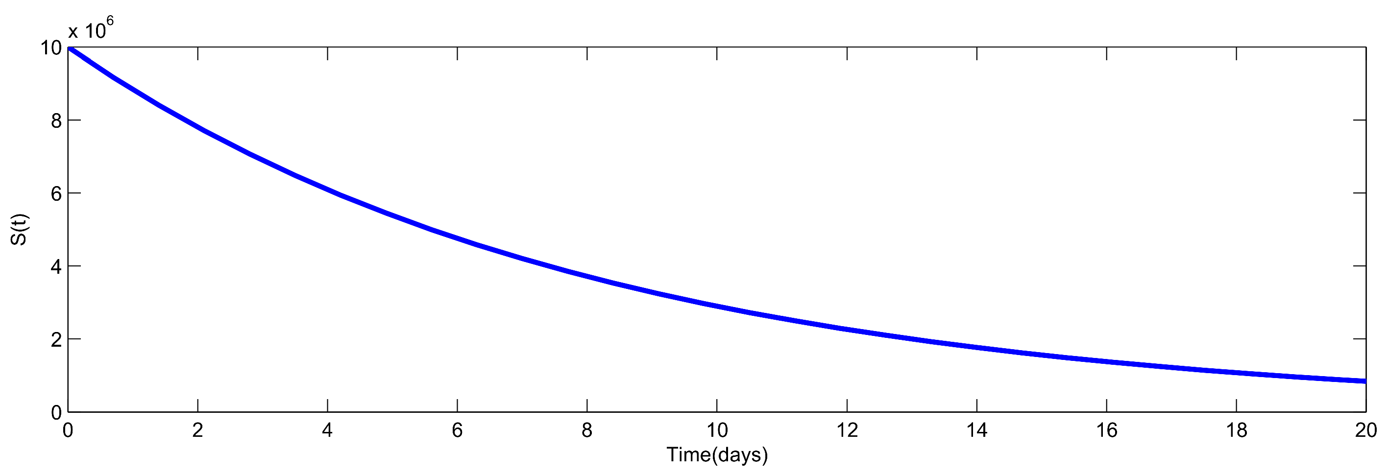
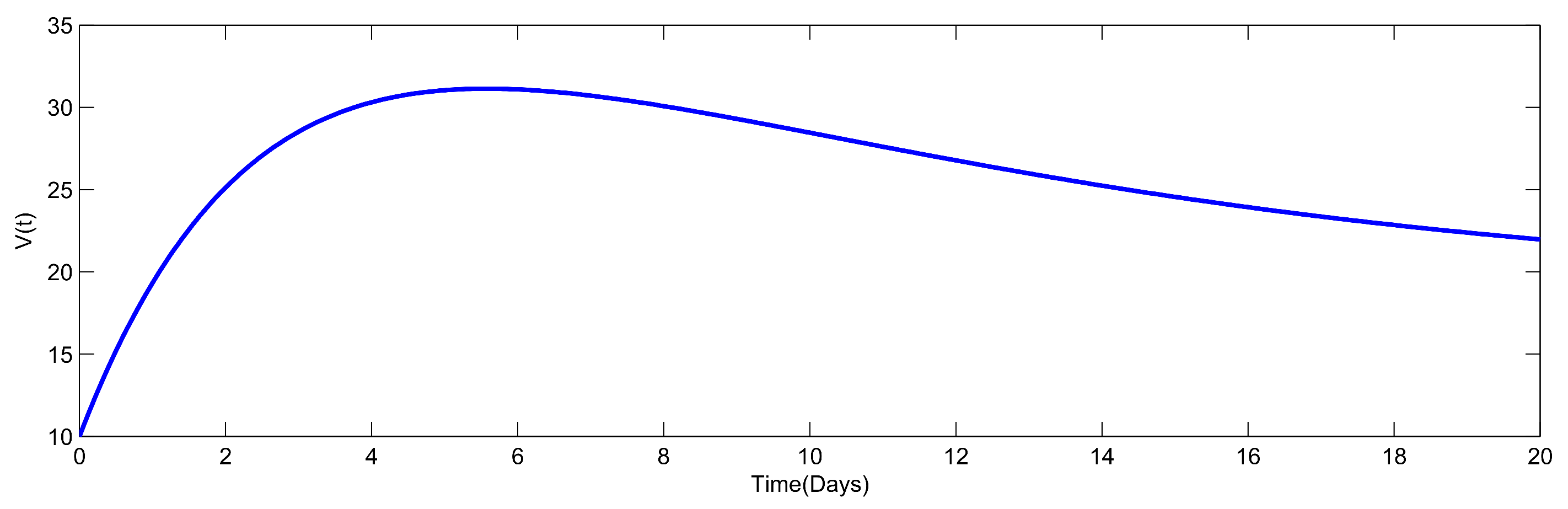
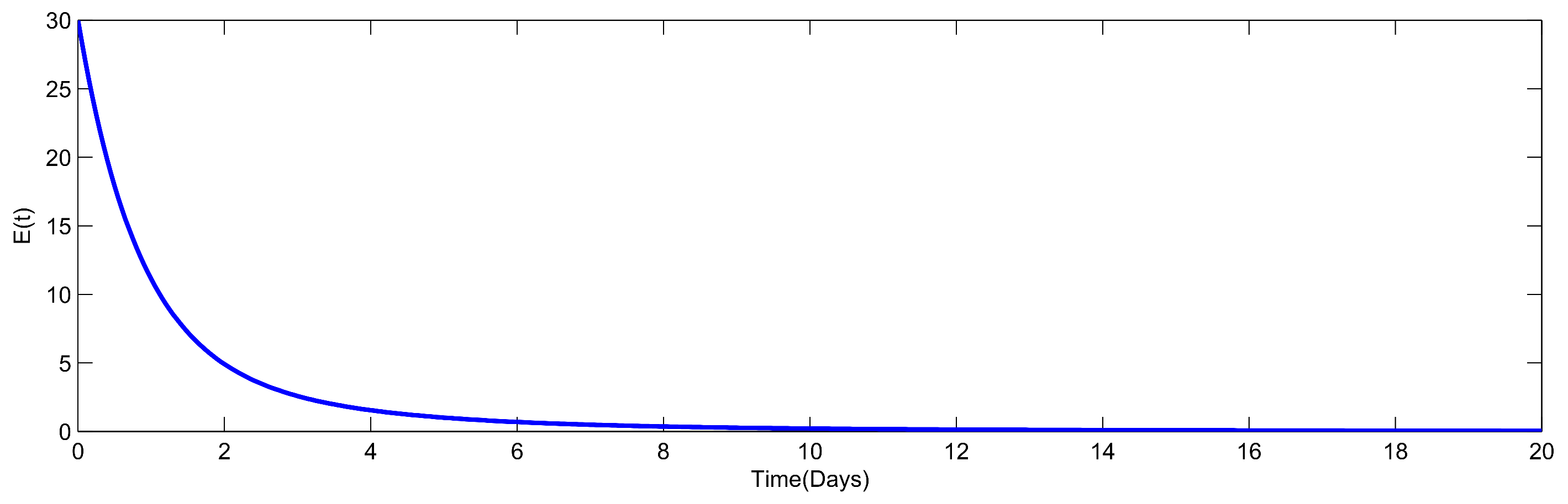
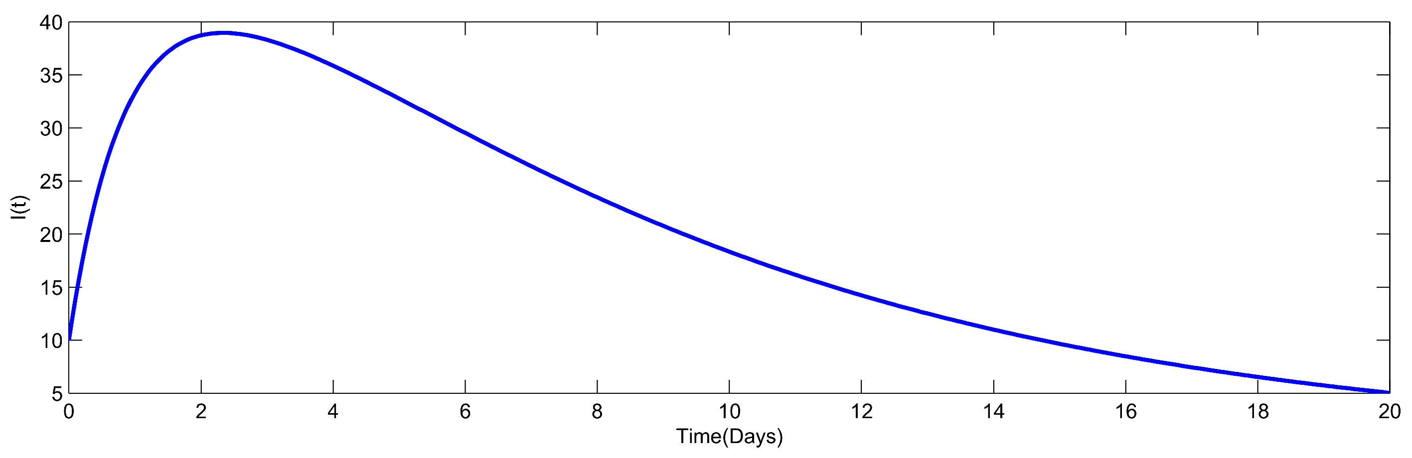
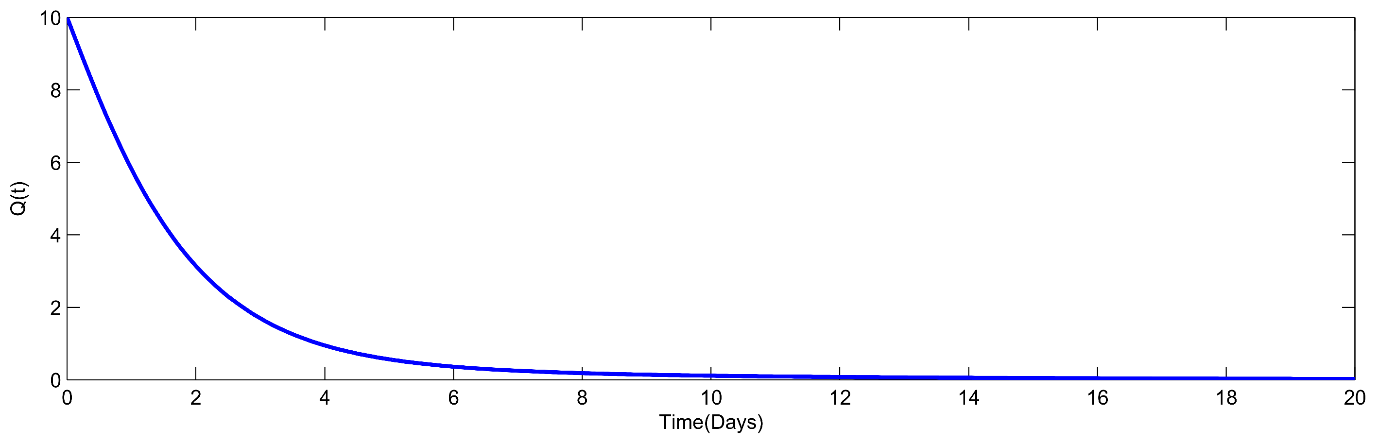
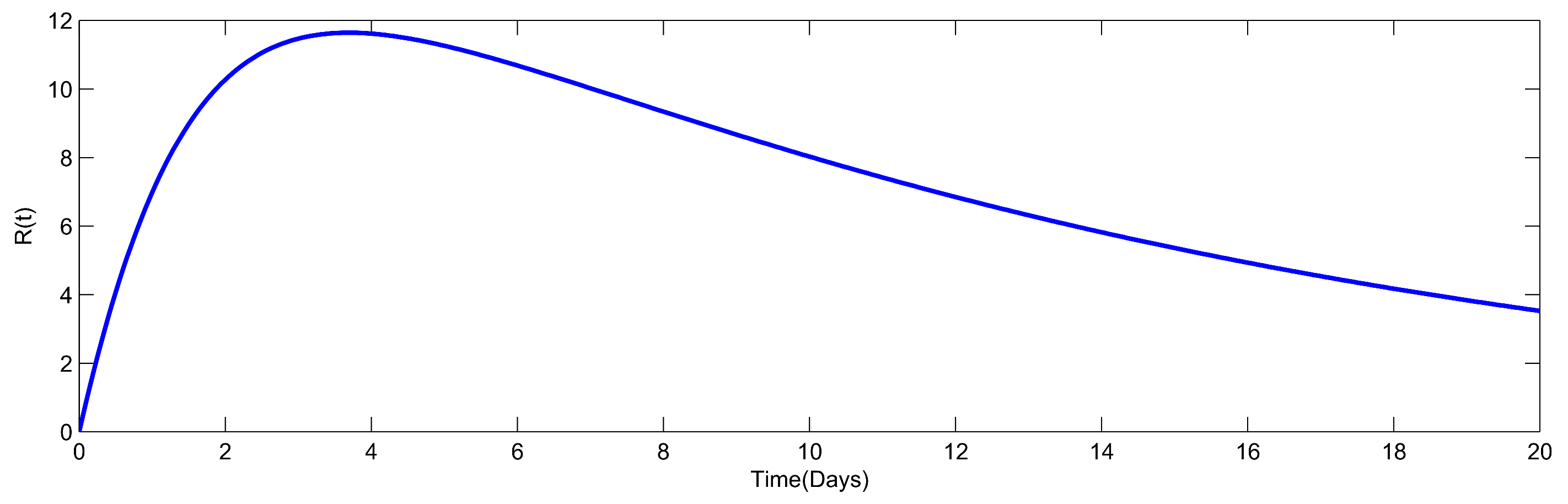
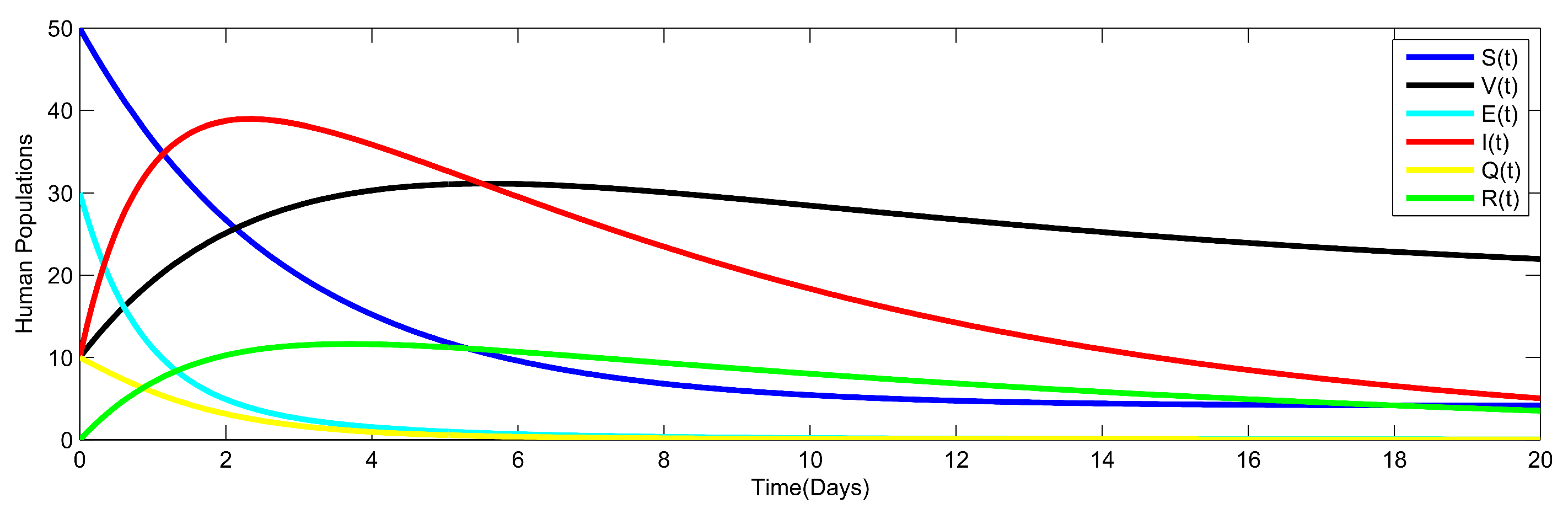
This part provides a graphical description of the numerical findings for the suggested model. We used the proposed numerical simulation technique for this purpose, along with the parameter values presented in

Table 2. Parameters and their values.

Variables and Parameters	Values	References
$\tau$	0.46	[29]
$\mu$	0.0991	[29]
$\lambda$	0.3002	[29]
$\pi$	0.001	[30]
q	$\frac{1}{14}$	[30]
v	0.4	Fit
$\delta$	$\frac{1}{40}$	[29]
$\gamma$	0.999	[29]
$\alpha$	0.2	[29]
$\varpi$	0.005	[30]

. The initial values of the state variables are provided as follows: $N\left(0\right)=\mathrm{230,000,000}$ is the population size, and $S\left(0\right)=\mathrm{1,000,000}$, $E\left(0\right)=50$, and $V\left(0\right)=35$. The infected populations are $I\left(0\right)=32$, $Q\left(0\right)=10$, and $R\left(0\right)=15$. In Figure 3, Figure 4, Figure 5, Figure 6, Figure 7 and Figure 8, we give the plots for the various compartments of the developed model. Initially, the infection was spreading more and more, but strong pharmaceutical and non-pharmaceutical measures were implemented, which effectively controlled the disease.

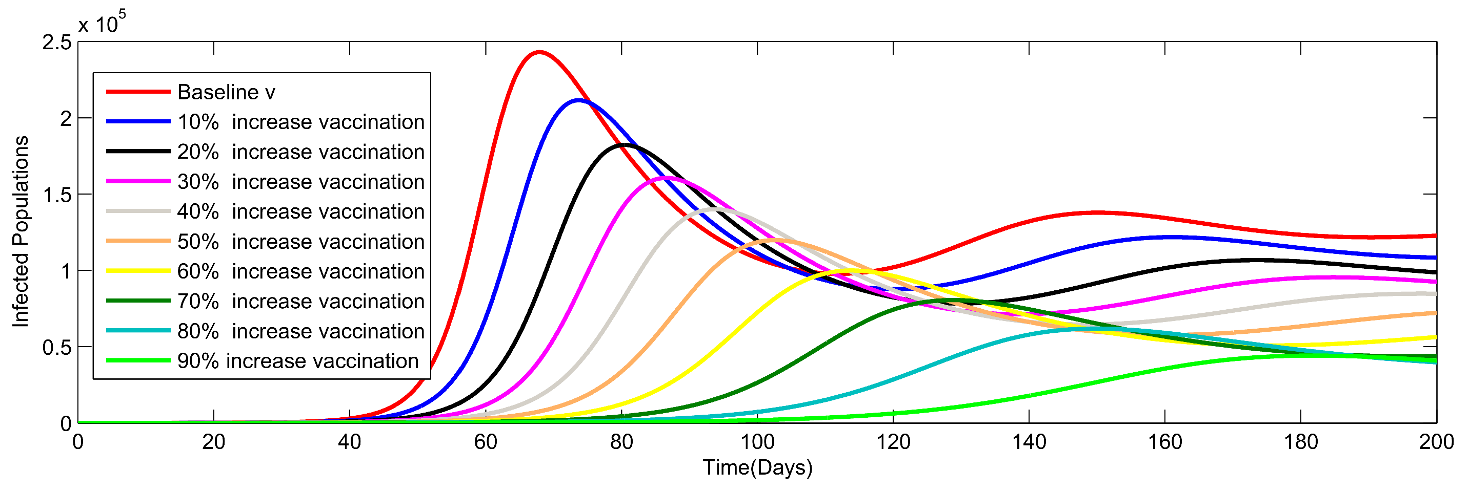
The plotting in the Figure 9 represents the dynamic of all compartments in the proposed model. It is clear from Figure 10 and Figure 11 that the value of the infected population declines as the vaccination compliance and efficiency rise. Additionally, if the vaccination is 100 percent effective in preventing disease transmission and is given in sufficient numbers, i.e., $\delta =1$, the value of ${\mathcal{R}}_0$ becomes zero, and the disease will not spread from one person to another in that scenario.

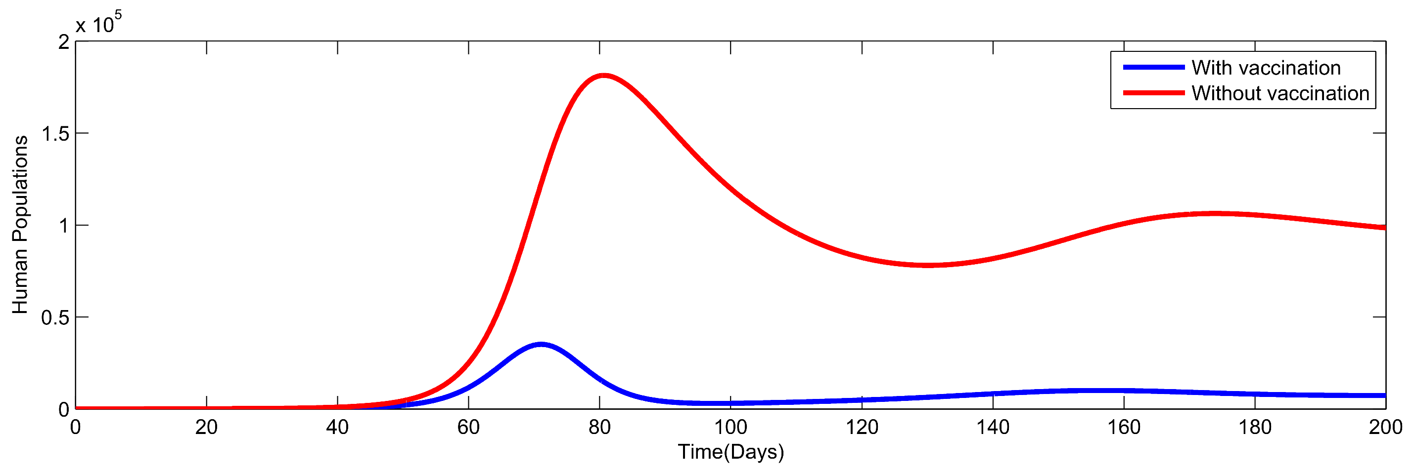
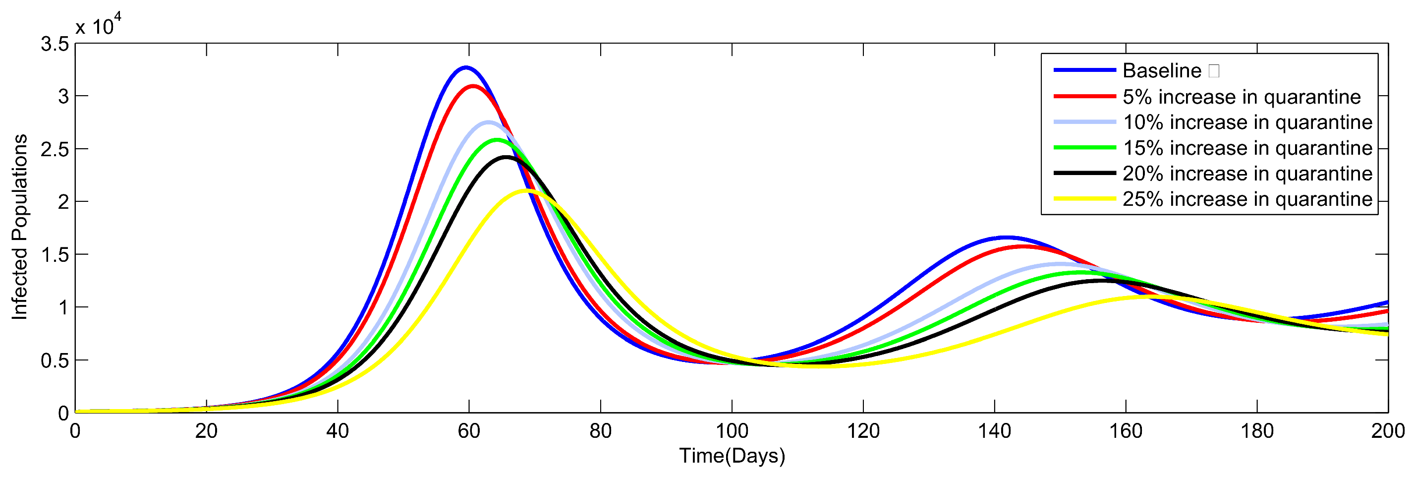
In order to investigate the dynamical impact of potential control actions on the incidence of infection in Pakistan, Figure 10, Figure 11, Figure 12, Figure 13 and Figure 14 are given. The simulation results are plotted for 200 and 300 days. We took into account several non-pharmaceutical techniques with their baseline values in the shown visual findings. The effect of the vaccine v, the proportion of persons who were exposed to and came into contact with COVID-19 patients, and finally, the combined impact of the vaccination and quarantine on the infected cases were the key areas of emphasis and analysis. The resultant graphical interpretation is shown in Figure 11, which demonstrates that, during the peak of the epidemic, 15,000 additional COVID-19 infections were anticipated. Additionally, Figure 11 describes that a considerable drop in COVID-19 occurs when vaccination efficacy is raised above the baseline values.

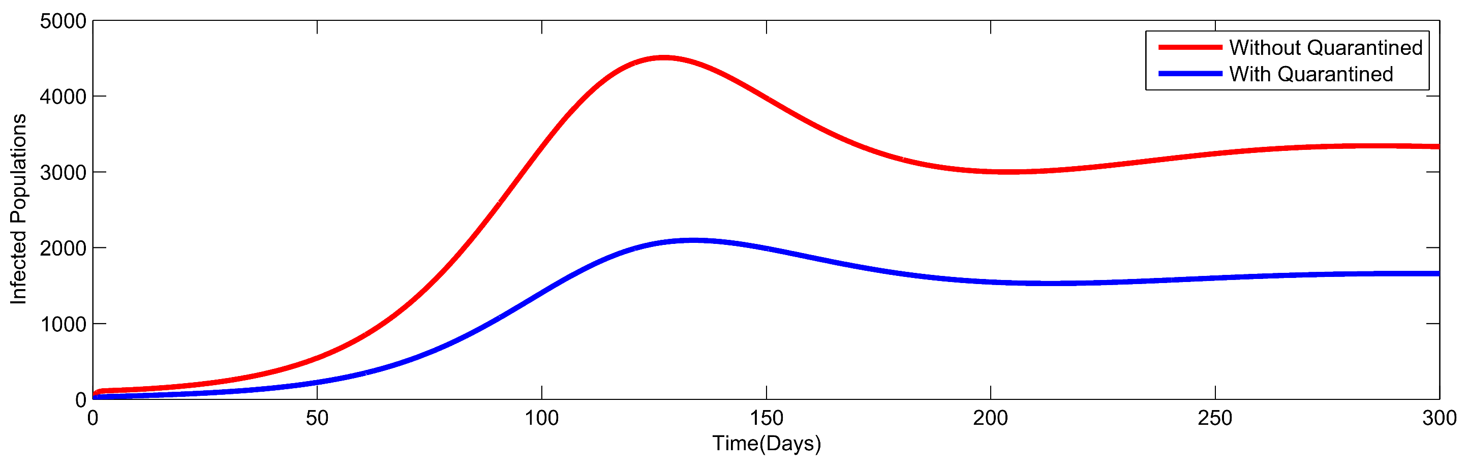
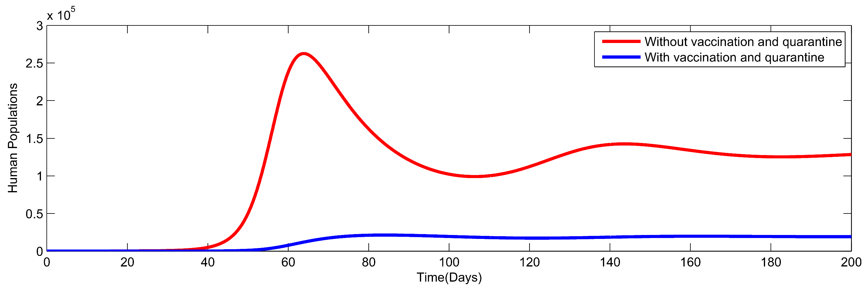
In Figure 11 and Figure 13, the dynamics of the new COVID-19 infected cases without and with the quarantine rate are shown. It is important to note that without quarantine, the situation is much worse and the number of infected patients unexpectedly increased (approximately 300,000). However, the peak number of new COVID-19 cases was drastically reduced when quarantine rates were only implemented at the baseline levels. In Figure 14, we further track the dynamics of infected cases without and with vaccination and quarantine. Note that the highest number of new COVID-19 cases increased to 290,000 without vaccination and quarantine and decreased to 15,000 with vaccination and quarantine. The use of both vaccination and quarantine was extremely successful and considerably decreased the number of instances of infection that were recorded.

9. Conclusions

We created a vaccination model by including the vaccine class and other factors that are crucial for immunizing those who are susceptible. First, we developed the model and gave the specific model outcomes. We examined the model’s stability at a disease-free equilibrium and discovered that it was locally asymptotically stable when ${\mathcal{R}}_0<1$, but the endemic equilibrium point was globally asymptotically stable when ${\mathcal{R}}_0>1$. We utilized the PRCC to obtain the model’s sensitivity analysis. Graphical representations of certain key parameters and their impact on the system were provided. In order to better understand the implications of these characteristics, we also provided some valuable data for vaccination and quarantine. The graphical interpretation supports the efficient use of vaccination and quarantining proven infected persons, which significantly lowered the number of infected people. Furthermore, were note that, without vaccines and quarantine, the disease situation was much worse and the number of infected patients rose quickly. The current research thus implies that, in order to prevent or reduce COVID-19 infection, adequate and effective implementation of these pharmaceutical and non-pharmaceutical therapies is still required.

References

- World Health Organization. Coronavirus Disease 2019 (COVID-19): Situation Report—99; World Health Organization: Geneva, Switzerland, 2020. [Google Scholar]
- World Health Organization. Coronavirus Disease 2019 (COVID-19): Situation Report—73; World Health Organization: Geneva, Switzerland, 2020. [Google Scholar]
- Trawicki, M.B. Deterministic seirs epidemic model for modeling vital dynamics, vaccinations, and temporary immunity. Mathematics 2017, 5, 7. [Google Scholar] [CrossRef] [Green Version]
- Din, A.; Shah, K.; Seadawy, A.; Alrabaiah, H.; Baleanu, D. On a new conceptual mathematical model dealing the current novel Coronavirus-19 infectious disease. Results Phys. 2020, 19, 103510. [Google Scholar] [CrossRef] [PubMed]
- Haq, I.U.; Ali, N.; Ahmad, H.; Nofal, T.A. On the fractional-order mathematical model of COVID-19 with the effects of multiple non-pharmaceutical interventions. AIMS Math. 2022, 7, 16017–16036. [Google Scholar] [CrossRef]
- Haq, I.U.; Ali, N.; Nisar, K.S. An optimal control strategy and grünwald-letnikov finite-difference numerical scheme for the fractional-order COVID-19 model. Math. Model. Numer. Simul. Appl. 2022, 2, 108–116. [Google Scholar] [CrossRef]
- Din, A.; Li, Y.; Khan, T.; Zaman, G. Mathematical analysis of spread and control of the novel corona virus (COVID-19) in China. Chaos Solitons Fractals 2020, 141, 110286. [Google Scholar] [CrossRef]
- Chen, Y.; Bi, K.; Zhao, S.; Ben-Arieh, D.; Wu, C.-H.J. Modeling individual fear factor with optimal control in a disease-dynamic system. Chaos Solitons Fractals 2017, 104, 531–545. [Google Scholar] [CrossRef]
- Hsieh, Y.-H. Middle East respiratory syndrome Coronavirus (mers-cov) nosocomial outbreak in South Korea: Insights from modeling. PeerJ 2015, 3, e1505. [Google Scholar] [CrossRef] [Green Version]
- Kim, Y.; Lee, S.; Chu, C.; Choe, S.; Hong, S.; Shin, Y. The characteristics of middle eastern respiratory syndrome coronavirus transmission dynamics in south korea. Osong Public Health Res. Perspect. 2016, 7, 49–55. [Google Scholar] [CrossRef] [Green Version]
- Bi, K.; Chen, Y.; Wu, C.-H.J.; Ben-Arieh, D. A memetic algorithm for solving optimal control problems of zika virus epidemic with equilibriums and backward bifurcation analysis. Commun. Nonlinear Sci. Numer. Simul. 2020, 84, 105176. [Google Scholar] [CrossRef]
- Chen, C.; Hsiao, C. Haar wavelet method for solving lumped and distributed-parameter systems. IEEE Proc.-Control Theory Appl. 1997, 144, 87–94. [Google Scholar] [CrossRef]
- Aziz, I. New algorithms for the numerical solution of nonlinear fredholm and volterra integral equations using haar wavelets. J. Comput. Appl. Math. 2013, 239, 333–345. [Google Scholar] [CrossRef]
- Lepik, Ü. Numerical solution of differential equations using haar wavelets. Math. Comput. Simul. 2005, 68, 127–143. [Google Scholar] [CrossRef]
- Lepik, Ü. Haar wavelet method for nonlinear integro-differential equations. Appl. Math. Comput. 2006, 176, 324–333. [Google Scholar] [CrossRef]
- Lepik, Ü. Solving pdes with the aid of two-dimensional haar wavelets. Comput. Math. Appl. 2011, 61, 1873–1879. [Google Scholar] [CrossRef] [Green Version]
- Lepik, Ü. Application of the haar wavelet transform to solving integral and differential equations. Proc. Est. Acad. Sci. Phys. Math. 2007, 56, 28–46. [Google Scholar] [CrossRef]
- Lepik, Ü. Solving fractional integral equations by the haar wavelet method. Appl. Math. Comput. 2009, 214, 468–478. [Google Scholar] [CrossRef]
- Majak, J.; Pohlak, M.; Eerme, M. Application of the haar wavelet-based discretization technique to problems of orthotropic plates and shells. Mech. Compos. Mater. 2009, 45, 631–642. [Google Scholar] [CrossRef]
- Jain, S. Numerical analysis for the fractional diffusion and fractional buckmaster equation by the two-step laplace adam-bashforth method. Eur. Phys. J. Plus 2018, 133, 1–11. [Google Scholar] [CrossRef]
- Rihan, F.; Al-Mdallal, Q.; AlSakaji, H.; Hashish, A. A fractional-order epidemic model with time-delay and nonlinear incidence rate. Chaos Solitons Fractals 2019, 126, 97–105. [Google Scholar] [CrossRef]
- Hajji, M.A.; Al-Mdallal, Q. Numerical simulations of a delay model for immune system-tumor interaction. Sultan Qaboos Univ. J. Sci. 2018, 23, 19–31. [Google Scholar] [CrossRef]
- Lai, C.-C.; Shih, T.-P.; Ko, W.-C.; Tang, H.-J.; Hsueh, P.-R. Severe acute respiratory syndrome coronavirus 2 (Sars-Cov-2) and Coronavirus disease-2019 (COVID-19): The epidemic and the challenges. Int. J. Antimicrob. Agents 2020, 55, 105924. [Google Scholar] [CrossRef]
- Babaaghaie, A.; Maleknejad, K. Numerical solutions of nonlinear two-dimensional partial volterra integro-differential equations by haar wavelet. J. Comput. Appl. Math. 2017, 317, 643–651. [Google Scholar] [CrossRef]
- Li, Y.; Zhao, W. Haar wavelet operational matrix of fractional order integration and its applications in solving the fractional order differential equations. Appl. Math. Comput. 2010, 216, 2276–2285. [Google Scholar] [CrossRef]
- Van den Driessche, P.; Watmough, J. Reproduction numbers and sub-threshold endemic equilibria for compartmental models of disease transmission. Math. Biosci. 2002, 180, 29–48. [Google Scholar] [CrossRef] [PubMed]
- Islam, R. Mathematical Analysis of Epidemiological Model of Virus Transmission Dynamics in Perspective of Bangladesh. Ph.D. Thesis, Khulna University of Engineering & Technology (KUET), Khulna, Bangladesh, 2018. [Google Scholar]
- Majak, J.; Shvartsman, B.; Karjust, K.; Mikola, M.; Haavajõe, A.; Pohlak, M. On the accuracy of the haar wavelet discretization method. Compos. Part B Eng. 2015, 80, 321–327. [Google Scholar] [CrossRef]
- Yavuz, M.; Coşar, F.Ö.; Günay, F.; Özdemir, F.N. A new mathematical modeling of the COVID-19 pandemic including the vaccination campaign. Open J. Model. Simul. 2021, 9, 299–321. [Google Scholar] [CrossRef]
- Diagne, M.; Rwezaura, H.; Tchoumi, S.; Tchuenche, J. A mathematical model of COVID-19 with vaccination and treatment. Comput. Math. Methods Med. 2021, 2021, 1250129. [Google Scholar] [CrossRef]
Figure 1.
Flow diagram of the model.
Figure 2.
Sensitivity indices for with respect to Model (1)’s parameter values.
Figure 3.
Dynamical representations of the susceptible class of Model (1).
Figure 4.
Dynamical representations of the vaccination class of Model (1).
Figure 5.
Dynamical representations of the exposed class of Model (1).
Figure 6.
Dynamical representations of the infected class of Model (1).
Figure 7.
Dynamical representations of the quarantined class of Model (1).
Figure 8.
Dynamical representations of the recovered class of Model (1).
Figure 9.
Graphical representations of Model (1).
Figure 10.
Graphical representations of Model (1) with the effect of different rates of vaccination.
Figure 11.
Graphical representation of Model (1) with and without the effect of vaccination.
Figure 12.
Graphical representation of Model (1) with and without the effect of quarantine.
Figure 13.
Graphical representation of Model (1) with the increasing effect of the quarantine rate.
Figure 14.
Graphical representation of Model (1) with the effect of vaccination and quarantine.