Darboux Transformation and Soliton Solution of the Nonlocal Generalized Sasa–Satsuma Equation

Abstract

This paper aims to seek soliton solutions for the nonlocal generalized Sasa–Satsuma (gSS) equation by constructing the Darboux transformation (DT). We obtain soliton solutions for the nonlocal gSS equation, including double-periodic wave, breather-like, KM-breather solution, dark-soliton, W-shaped soliton, M-shaped soliton, W-shaped periodic wave, M-shaped periodic wave, double-peak dark-breather, double-peak bright-breather, and M-shaped double-peak breather solutions. Furthermore, interaction of these solitons, as well as their dynamical properties and asymptotic analysis, are analyzed. It will be shown that soliton solutions of the nonlocal gSS equation can be reduced into those of the nonlocal Sasa–Satsuma equation. However, several of these properties for the nonlocal Sasa–Satsuma equation are not found in the literature.

1. Introduction

Ablowitz and Musslimani proposed the nonlocal reverse space nonlinear Schrödinger (NLS) equation [1]

$$\mathrm{i}{q}_t(x,t)+q_{xx}(x,t)\pm 2q^2(x,t)q^{*}(-x,t)=0,$$

(1)

where * denotes a complex conjugate. Soliton solutions to Equation (1) have been discussed by inverse scattering transform and Darboux transformation [1,2,3,4,5]. It is interesting that the nonlocal NLS equation has many properties different from the NLS equation, e.g., the nonlocal NLS equation can simultaneously exist as both bright and dark solitons [3] and has solutions with periodic singularities [1]. Since then, the research on integrable nonlocal equations, including nonlocal reverse space, nonlocal reverse time, and nonlocal reverse space–time, has received more and more attention. Nonlocal versions of many important integrable equations have been studied, such as the nonlocal sine Gordon equation [2], nonlocal mKdV equation [6,7], nonlocal complex mKdV equation [8], nonlocal Sasa–Satsuma equation [9], nonlocal Davey–Stewartson equation [10,11], etc.

Very recently, Geng and Wu introduced a generalized Sasa–Satsuma equation [12]

$$u_t+u_{xxx}-{3(2a|u|}^2{u}_x+2b{u}^2{u}_x+{au(|u|}^2{)}_x+b^{*}{u}^{*}{(|u|}^2{)}_x)=0,$$

(2)

where a is real constant and b is complex constant satisfying $|a|\ne |b|$. Soliton solutions by the Riemann–Hilbert method and long-time asymptotic behavior of Equation (2) were studied in [12,13]. Under the variable transformations

$$u(x,t)=q(X,T)\exp \left\{-\frac{\mathrm{i}}{6}(X-\frac{T}{18})\right\},t=T,x=X-\frac{T}{12},$$

(3)

gSS Equation (2) becomes

$$\begin{array}{ccc}\hfill & & \mathrm{i}{q}_{{}_T}+\frac{1}{2}{q}_{{}_{XX}}-{aq|q|}^2+\mathrm{i}{q}_{{}_{XXX}}-3\mathrm{i}a(2q_{{}_X}{|q|}^2+{q(|q|}^2{)}_{{}_X})\hfill \\ \hfill & & -3\mathrm{i}{\mathrm{e}}^{\frac{\mathrm{i}}{3}(X-\frac{T}{18})}\left(b{\mathrm{e}}^{-\frac{2\mathrm{i}}{3}(X-\frac{T}{18})}(2q^2{q}_{{}_X}-\frac{\mathrm{i}}{3}{q}^3)+b^{*}{q}^{*}{(|q|}^2{)}_{{}_X}\right)=0,\hfill \end{array}$$

(4)

It is obvious that Equation (4) with $b=0$ is just the Sasa–Satsuma equation [14]. As a high-order NLS equation, the Sasa–Satsuma equation describes the propagation of femtosecond pulses in optical fibers [15]. Equation (2) is really a generalized Sasa–Satsuma equation. Inspired by the research work of the nonlocal NLS equation and nonlocal Sasa–Satsuma equation, in this paper, we investigate the following nonlocal generalized Sasa–Satsuma equation:

$$u_t+u_{xxx}-3ϵ[2au{u}_x{u}^{*}(-x,-t)+au{\left(u{u}^{*}(-x,-t)\right)}_x+2b{u}^2{u}_x+b^{*}{u}^{*}(-x,-t){\left(u{u}^{*}(-x,-t)\right)}_x]=0,$$

(5)

where $aϵ=-1$ represents the focusing case, and $aϵ=1$ stands for the defocusing case. The nonlocal generalized Sasa–Satsuma Equation (5) was proposed in ref. [16], in which the soliton solution of nonlocal integrable equation

$$q_t+q_{xxx}+3aq({\left(qq(-x,-t)\right)}_x+2q_{x}q(-x,-t))-6b{q}^2{q}_x-3b^{*}q(-x,-t){\left(qq(-x,-t)\right)}_x=0$$

is obtained by the Riemann–Hilbert method. It is clear that the nonlocal gSS Equation (5) is different from the last equation. We will construct Darboux transformation and soliton solutions for the nonlocal gSS equation. In Ref. [9], a nonlocal Sasa–Satsuma equation

$$u_t+u_{xxx}+3ϵ(2u{u}^{*}(-x,-t)u_x+u{\left(u{u}^{*}(-x,-t)\right)}_x)=0$$

(6)

was introduced and investigated. Its soliton solutions were obtained using the Darboux transformation, including dark soliton, W-shaped soliton, M-shaped soliton, and breather soliton. We should remark here that when $a=-1,b=0,$ the nonlocal gSS Equation (5) reduces to the nonlocal Sasa–Satsuma Equation (6); when $a=0,b=-1,$ the nonlocal gSS (5) can yield a new nonlocal complex modified KdV-type equation

$$u_t+u_{xxx}+3ϵ(2u^2{u}_x+u^{*}(-x,-t){\left(u{u}^{*}(-x,-t)\right)}_x)=0.$$

(7)

In this paper, we will give the constructions of the N-fold Darboux transformation and soliton solutions for the nonlocal gSS Equation (5), including double-periodic wave, breather-like, KM-breather solution, dark soliton, W-shaped soliton, M-shaped soliton, W-shaped periodic wave, M-shaped periodic wave, double-peak dark-breather, and bright-breather. Furthermore, interaction of these solitons, as well as their dynamical and asymptotic properties, are analyzed. The reduction of soliton solutions of nonlocal gSS Equation (5) yields the soliton solutions for nonlocal Sasa–Satsuma Equation (6) and nonlocal complex modified KdV-type Equation (7). We would emphasize here that breather-like, KM-breather, W-shaped periodic wave, M-shaped periodic wave, double-peak dark-breather, and double-peak bright-breather for the nonlocal Sasa–Satsuma Equation (6) have not been discussed in the literature.

This paper is organized as follows: In Section 2, the N-fold Darboux transformation of the nonlocal gSS Equation (5) is constructed. We obtain the soliton formulas for the nonlocal gSS equation. In Section 3, using the Darboux transformation, various 1-soliton and 2-soliton solutions for the nonlocal gSS equation are derived. Further, the dynamical and asymptotic behavior of these solutions are analyzed. Finally, Section 4 is devoted to conclusions.

2. Darboux Transformation for the Nonlocal gSS Equation (5)

In this section, we construct the N-fold Darboux transformation of the gSS Equation (5).

The linear spectral problem of the nonlocal gSS Equation (5) can be written as

$$\begin{array}{ccc}\hfill & & {\mathsf{\Psi }}_x=U(\lambda ,Q)\mathsf{\Psi },{\mathsf{\Psi }}_t=V(\lambda ,Q)\mathsf{\Psi },\hfill \\ \hfill & & U(\lambda ,Q)=\mathrm{i}\lambda \Lambda +Q,V(\lambda ,Q)=4\mathrm{i}{\lambda }^3\Lambda +4{\lambda }^{2}Q+2\mathrm{i}\lambda (Q^2+Q_x)\Lambda +Q_{x}Q-Q{Q}_x-Q_{xx}+2Q^3,\hfill \end{array}$$

(8)

where $\mathsf{\Psi }={({\psi }_1(x,t),{\psi }_2(x,t),{\psi }_3(x,t))}^T$ is an eigenfunction, $\lambda$ is the spectral parameter, and

$$\begin{array}{c}\hfill Q=\left(\begin{array}{ccc}0& 0& u\\ 0& 0& ϵu^{*}(-x,-t)\\ ϵ(a{u}^{*}(-x,-t)+bu)& au+b^{*}{u}^{*}(-x,-t)& 0\end{array}\right),\Lambda =\mathrm{diag}(1,1,-1).\end{array}$$

Suppose that $|y_j\rangle ={({\psi }_1^{\left(j\right)},{\psi }_2^{\left(j\right)},{\psi }_3^{\left(j\right)})}^T$ is an eigenfunction for the spectral problem (8) at $\lambda ={\lambda }_j$, then $|{\eta }_j\rangle ={({\tilde{\psi }}_2^{\left(j\right)},{\tilde{\psi }}_1^{\left(j\right)},-ϵ{\tilde{\psi }}_3^{\left(j\right)})}^{†}$ is also an eigenfunction of the spectral problem (8) at $\lambda ={\lambda }_j^{*}$, where † represents the complex conjugate transpose and ${\tilde{\psi }}_j={\psi }_j(-x,-t)$. It can be checked that $\langle {\theta }_j|=\langle y_j(-x,-t)|\mathbf{J}$ is an eigenfunction to the adjoint problem of Equation (5)

$$\langle {\theta }_j{|}_x=-\langle {\theta }_j|U,\langle {\theta }_j{|}_t=-\langle {\theta }_j|V$$

(9)

at $\lambda ={\lambda }_j^{*}$, where

$$\begin{array}{c}\hfill \mathbf{J}=\left(\begin{array}{ccc}aϵ& b^{*}& 0\\ b& aϵ& 0\\ 0& 0& 1\end{array}\right),\langle y_j(-x,-t)|=|y_j{\rangle }^{†}(-x,-t).\end{array}$$

We obtain our main result for the construction of the N-fold Darboux transformation to the nonlocal gSS Equation (5).

Theorem 1.

Under the gauge transformation

$$\begin{array}{c}\hfill {\mathsf{\Psi }}^{\left(N\right)}=T^{\left(N\right)}\mathsf{\Psi },T^{\left(N\right)}=I-{\mathbb{K}}_N{W}_N^{-1}\Gamma \left({\mathbb{K}}_N\right),\end{array}$$

(10)

where

$$\begin{array}{ccc}\hfill & & {\mathbb{K}}_N=(|y_1\rangle ,|{\eta }_1\rangle ,|y_2\rangle ,|{\eta }_2\rangle ,\cdots |y_N\rangle ,|{\eta }_N\rangle )\triangleq (K_1,K_2,\cdots ,K_N),\hfill \\ \hfill & & W_N=\left(\begin{array}{cc}\Omega (K_1,K_1)& \Omega (K_1,K_2)\cdots \Omega (K_1,K_N)\\ \Omega (K_2,K_2)& \Omega (K_2,K_2)\cdots \Omega (K_2,K_N)\\ ⋮& ⋮\ddots ⋮\\ \Omega (K_N,K_1)& \Omega (K_N,K_2)\cdots \Omega (K_N,K_N)\end{array}\right),\Gamma \left({\mathbb{K}}_N\right)=\left(\begin{array}{c}\Gamma \left(K_1\right)\\ \Gamma \left(K_2\right)\\ ⋮\\ \Gamma \left(K_N\right)\end{array}\right),\hfill \\ \hfill & & \Omega (K_k,K_j)=\left(\begin{array}{cc}\frac{\langle y_k(-x,-t)|\mathbf{J}|y_j\rangle }{-{\lambda }_k^{*}-{\lambda }_j}& \frac{\langle y_k(-x,-t)|\mathbf{J}|{\eta }_j\rangle }{-{\lambda }_k^{*}-{\lambda }_j^{*}}\\ \frac{\langle {\eta }_k(-x,-t)|\mathbf{J}|y_j\rangle }{-{\lambda }_k-{\lambda }_j}& \frac{\langle {\eta }_k(-x,-t)|\mathbf{J}|{\eta }_j\rangle }{-{\lambda }_k-{\lambda }_j^{*}}\end{array}\right),\Gamma \left(K_k\right)=\left(\begin{array}{c}\frac{\langle y_k(-x,-t)|\mathbf{J}}{-{\lambda }_k^{*}-\lambda }\\ \frac{\langle {\eta }_k(-x,-t)|\mathbf{J}}{-{\lambda }_k-\lambda }\end{array}\right),1\le k,j\le N,\hfill \end{array}$$

(11)

the spectral problem (8) converts into a new spectral problem

$${\mathsf{\Psi }}_x^{\left(N\right)}=U^{\left(N\right)}(\lambda ,Q^{\left(N\right)}){\mathsf{\Psi }}^{\left(N\right)},{\mathsf{\Psi }}_t^{\left(N\right)}=V^{\left(N\right)}(\lambda ,Q^{\left(N\right)}){\mathsf{\Psi }}^{\left(N\right)},$$

(12)

where

$$Q^{\left(N\right)}=Q+\mathrm{i}\left[{\mathbb{K}}_N{W}_N^{-1}{\tilde{\mathbb{K}}}_N^{†}\mathbf{J},\Lambda \right].$$

(13)

We can draw the conclusion that the structures of matrices $U^{\left(N\right)}(\lambda ,Q^{\left(N\right)})$, $V^{\left(N\right)}(\lambda ,Q^{\left(N\right)})$ are same as the matrices $U(\lambda ,Q)$, $V(\lambda ,Q)$. This means that $u(x,t)$ is a solution corresponding to eigenfunction ψ for the nonlocal gSS Equation (5), and then $u^{\left(N\right)}(x,t)$ is a solution corresponding to eigenfunction ${\psi }^{\left(N\right)}$ for the nonlocal gSS Equation (5). The relation between the potential $u^{\left(N\right)}(x,t)$ and the potential $u(x,t)$ is given by

$$u^{\left(N\right)}=u-2\mathrm{i}{\mathbf{h}}_1{W}_N^{-1}{\tilde{\mathbf{h}}}_3^{†},$$

(14)

where

$$\begin{array}{cc}\hfill & {\mathbf{h}}_1=({\psi }_1^{\left(1\right)},{\tilde{\psi }}_2^{{\left(1\right)}^{*}},{\psi }_1^{\left(2\right)},{\tilde{\psi }}_2^{{\left(2\right)}^{*}},\cdots ,{\psi }_1^{\left(N\right)},{\tilde{\psi }}_2^{{\left(N\right)}^{*}}),\hfill \\ \hfill & {\mathbf{h}}_3=({\psi }_3^{\left(1\right)},-ϵ{\tilde{\psi }}_3^{{\left(1\right)}^{*}},{\psi }_3^{\left(2\right)},-ϵ{\tilde{\psi }}_3^{{\left(2\right)}^{*}},\cdots ,{\psi }_3^{\left(N\right)},-ϵ{\tilde{\psi }}_3^{{\left(N\right)}^{*}}).\hfill \end{array}$$

Proof. 

Through a direct calculation, we have $\Lambda \mathbf{J}=\mathbf{J}\Lambda$, ${\tilde{Q}}^{†}\mathbf{J}=\mathbf{J}Q$ and $\Lambda Q=-Q\Lambda$. Then we can verify following equations:

$$\begin{array}{ccc}& & (\langle y_k(-x,-t)|\mathbf{J}|y_j{\rangle )}_x=\mathrm{i}({\lambda }_k^{*}+{\lambda }_j)\langle y_k(-x,-t)|\mathbf{J}\Lambda |y_j\rangle ,\hfill \\ & & (\langle y_k(-x,-t)|\mathbf{J}|{\eta }_j{\rangle )}_x=\mathrm{i}({\lambda }_k^{*}+{\lambda }_j^{*})\langle y_k(-x,-t)|\mathbf{J}\Lambda |y_j\rangle ,\hfill \\ & & (\langle {\eta }_k(-x,-t)|\mathbf{J}|y_j{\rangle )}_x=\mathrm{i}({\lambda }_k+{\lambda }_{\mathrm{i}})\langle {\eta }_k(-x,-t)|\mathbf{J}\Lambda |y_j\rangle ,\hfill \\ & & (\langle {\eta }_k(-x,-t)|\mathbf{J}|{\eta }_j{\rangle )}_x=\mathrm{i}({\lambda }_k+{\lambda }_j^{*})\langle {\eta }_k(-x,-t)|\mathbf{J}\Lambda |y_j\rangle ,k,j=1,2,3,...N.\hfill \end{array}$$

With a direct calculation, we have

$$\begin{array}{ccc}\hfill & & D_N^{†}\Gamma \left({\mathbb{K}}_N\right)+\lambda \Gamma \left({\mathbb{K}}_N\right)=-{\tilde{\mathbb{K}}}_N^{†}\mathbf{J},W_N{D}_N^{†}+D_N{W}_N=-W_N^{-1}{\tilde{\mathbb{K}}}_N^{†}\mathbf{J}{\mathbb{K}}_N{W}_N^{-1},\hfill \\ \hfill & & {\mathbb{K}}_{N,x}=\mathrm{i}\Lambda {\mathbb{K}}_N{D}_N+Q{\mathbb{K}}_N,{(\Gamma \left({\mathbb{K}}_N\right)\mathsf{\Psi })}_x=-\mathrm{i}{\tilde{\mathbb{K}}}_N^{†}(-x,-t)\mathbf{J}\Lambda \mathsf{\Psi },\hfill \\ \hfill & & W_{N,x}=-\mathrm{i}{\tilde{\mathbb{K}}}_N^{†}(-x,-t)\mathbf{J}\Lambda {\mathbb{K}}_N,D_N=\mathrm{diag}({\lambda }_1,{\lambda }_1^{*},{\lambda }_2,{\lambda }_2^{*},...,{\lambda }_N,{\lambda }_N^{*}),\hfill \end{array}$$

(15)

and then we get

$$\begin{array}{ccc}& & {\mathsf{\Psi }}_x^{\left(N\right)}=(\mathrm{i}\lambda \Lambda +Q)\mathsf{\Psi }-{\mathbb{K}}_{N,x}{W}_N^{-1}\Gamma \left({\mathbb{K}}_N\right)\mathsf{\Psi }-{\mathbb{K}}_N{W}_N^{-1}{(\Gamma \left({\mathbb{K}}_N\right)\mathsf{\Psi })}_x+{\mathbb{K}}_N{W}_N^{-1}{W}_{N,x}{W}_N^{-1}\Gamma \left({\mathbb{K}}_1\right)\mathsf{\Psi }\hfill \\ & & =(\mathrm{i}\lambda \Lambda +Q)\mathsf{\Psi }-\mathrm{i}\Lambda {\mathbb{K}}_N{D}_N{W}_N^{-1}\Gamma \left({\mathbb{K}}_N\right)\mathsf{\Psi }-Q{\mathbb{K}}_N{W}_N^{-1}\Gamma \left({\mathbb{K}}_N\right)\mathsf{\Psi }+\mathrm{i}{\mathbb{K}}_N{W}_N^{-1}{\tilde{\mathbb{K}}}_N^{†}\mathbf{J}\Lambda \mathsf{\Psi }\hfill \\ & & -\mathrm{i}{\mathbb{K}}_N{W}_N^{-1}{\tilde{\mathbb{K}}}_N^{†}\mathbf{J}\Lambda {\mathbb{K}}_N{W}_N^{-1}\Gamma \left({\mathbb{K}}_N\right)\mathsf{\Psi }\hfill \\ & & =(\mathrm{i}\lambda \Lambda +Q)\mathsf{\Psi }+\mathrm{i}\Lambda {\mathbb{K}}_N(W_N^{-1}{\tilde{\mathbb{K}}}_N^{†}\mathbf{J}{\mathbb{K}}_N{W}_N^{-1}+W_N^{-1}{D}_N^{†})\Gamma \left({\mathbb{K}}_N\right)\mathsf{\Psi }-Q{\mathbb{K}}_N{W}_N^{-1}\Gamma \left({\mathbb{K}}_N\right)\mathsf{\Psi }\hfill \\ & & +\mathrm{i}{\mathbb{K}}_N{W}_N^{-1}{\tilde{\mathbb{K}}}_N^{†}\mathbf{J}\Lambda \mathsf{\Psi }-\mathrm{i}{\mathbb{K}}_N{W}_N^{-1}{\tilde{\mathbb{K}}}_N^{†}\mathbf{J}\Lambda {\mathbb{K}}_N{W}_N^{-1}\Gamma \left({\mathbb{K}}_N\right)\mathsf{\Psi }\hfill \\ & & =(\mathrm{i}\lambda \Lambda +Q)\mathsf{\Psi }-Q{\mathbb{K}}_N{W}_N^{-1}\Gamma \left({\mathbb{K}}_N\right)\mathsf{\Psi }+\mathrm{i}\Lambda {\mathbb{K}}_N{W}_N^{-1}{\tilde{\mathbb{K}}}_N^{†}\mathbf{J}{\mathbb{K}}_N{W}_N^{-1}\Gamma \left({\mathbb{K}}_N\right)\mathsf{\Psi }-\mathrm{i}\lambda \Lambda {\mathbb{K}}_N{W}_N^{-1}\Gamma \left({\mathbb{K}}_N\right)\mathsf{\Psi }\hfill \\ & & -\mathrm{i}\Lambda {\mathbb{K}}_N{W}_N^{-1}{\tilde{\mathbb{K}}}_N^{†}\mathbf{J}\mathsf{\Psi }+\mathrm{i}{\mathbb{K}}_N{W}_N^{-1}{\tilde{\mathbb{K}}}_N^{†}\mathbf{J}\Lambda \mathsf{\Psi }-\mathrm{i}{\mathbb{K}}_N{W}_N^{-1}{\tilde{\mathbb{K}}}_N^{†}\mathbf{J}\Lambda {\mathbb{K}}_N{W}_N^{-1}\Gamma \left({\mathbb{K}}_N\right)\mathsf{\Psi }\hfill \\ & & =(\mathrm{i}\lambda \Lambda +Q+\mathrm{i}{\mathbb{K}}_N{W}_N^{-1}{\tilde{\mathbb{K}}}_N^{†}\mathbf{J}\Lambda -\mathrm{i}\Lambda {\mathbb{K}}_N{W}_N^{-1}{\tilde{\mathbb{K}}}_N^{†}\mathbf{J})(I-{\mathbb{K}}_N{W}_N^{-1}\Gamma \left({\mathbb{K}}_N\right))\mathsf{\Psi }\hfill \\ & & =(\mathrm{i}\lambda \Lambda +Q^{\left(N\right)}){\mathsf{\Psi }}^{\left(N\right)}=U^{\left(N\right)}{\mathsf{\Psi }}^{\left(N\right)}.\hfill \end{array}$$

Let us show that the potential $Q^{\left(N\right)}$ has the same structure with the potential Q. Taking $\Theta ={\mathbb{K}}_N{W}_N^{-1}{\mathbb{K}}_N^{†}\mathbf{J}$, Equation (13) can be rewritten as

$$Q^{\left(N\right)}=\left(\begin{array}{ccc}0& 0& u-2\mathrm{i}{\Theta }_{13}\\ 0& 0& ϵu^{*}(-x,-t)-2\mathrm{i}{\Theta }_{23}\\ ϵ(a{u}^{*}(-x,-t)+bu)+2\mathrm{i}{\Theta }_{31}& au+b^{*}{u}^{*}(-x,-t)+2\mathrm{i}{\Theta }_{32}& 0\end{array}\right),$$

where

$$\begin{array}{ccc}& & {\Theta }_{13}=-\frac{\left|\begin{array}{cc}{W}_N& {\tilde{\mathbf{h}}}_3^{†}\\ {\mathbf{h}}_1& 0\end{array}\right|}{|W_N|},{\Theta }_{31}=-\frac{ϵa\left|\begin{array}{cc}{W}_N& {\tilde{\mathbf{h}}}_1^{†}\\ {\mathbf{h}}_3& 0\end{array}\right|+b\left|\begin{array}{cc}{W}_N& {\tilde{\mathbf{h}}}_2^{†}\\ {\mathbf{h}}_3& 0\end{array}\right|}{|W_N|},\hfill \\ \hfill & & {\Theta }_{23}=-\frac{\left|\begin{array}{cc}{W}_N& {\tilde{\mathbf{h}}}_3^{†}\\ {\mathbf{h}}_2& 0\end{array}\right|}{|W_N|},{\Theta }_{32}=-\frac{b^{*}\left|\begin{array}{cc}{W}_N& {\tilde{\mathbf{h}}}_1^{†}\\ {\mathbf{h}}_3& 0\end{array}\right|+ϵa\left|\begin{array}{cc}{W}_N& {\tilde{\mathbf{h}}}_2^{†}\\ {\mathbf{h}}_3& 0\end{array}\right|}{|W_N|},\hfill \end{array}$$

with

$$\begin{array}{c}\hfill {\mathbf{h}}_2=({\psi }_2^{\left(1\right)},{\tilde{\psi }}_1^{{\left(1\right)}^{*}},{\psi }_2^{\left(2\right)},{\tilde{\psi }}_1^{{\left(2\right)}^{*}},\cdots ,{\psi }_2^{\left(N\right)},{\tilde{\psi }}_1^{{\left(N\right)}^{*}}).\end{array}$$

Note that

$$\begin{array}{cc}\hfill & \langle {\eta }_k(-x,-t)|\mathbf{J}|{\eta }_j\rangle =\langle y_j(-x,-t)|\mathbf{J}|y_k\rangle ,\hfill \\ \hfill & \langle {\eta }_k(-x,-t)|\mathbf{J}|y_j\rangle =\langle {\eta }_j(-x,-t)|\mathbf{J}|y_k\rangle ,\hfill \\ \hfill & \langle y_k(-x,-t)|\mathbf{J}|{\eta }_j\rangle =\langle y_j(-x,-t)|\mathbf{J}|{\eta }_k\rangle ,\hfill \end{array}$$

we thus have $\Omega (K_k,K_j)=\tilde{\Omega }{(K_j,K_k)}^{†}$ and $W_N={\tilde{W}}_N^{†}$. By setting a $2N\times 2N$ permutation matrix

$$A=\left(\begin{array}{ccccc}0& 1& \cdots & 0& 0\\ 1& 0& \cdots & 0& 0\\ ⋮& ⋮& \ddots & ⋮& ⋮\\ 0& 0& \cdots & 0& 1\\ 0& 0& \cdots & 1& 0\end{array}\right),$$

we have ${\mathbf{h}}_2={\tilde{\mathbf{h}}}_{1}A,{\mathbf{h}}_3=-ϵ{\tilde{\mathbf{h}}}_{3}A$ and $A{W}_{N}A=W_N^T$. With these identities, we obtain

$$\begin{array}{ccc}& & \left|\begin{array}{cc}{W}_N& {\tilde{\mathbf{h}}}_3^{†}\\ {\mathbf{h}}_2& 0\end{array}\right|=\left|\begin{array}{cc}A{W}_N^{T}A& -ϵA{\mathbf{h}}_3^T\\ {\mathbf{h}}_1^{*}A& 0\end{array}\right|=\left|\begin{array}{cc}{W}_N^T& -ϵ{\mathbf{h}}_3^T\\ {\tilde{\mathbf{h}}}_1^{*}& 0\end{array}\right|=-ϵ\left|\begin{array}{cc}{W}_N& {\tilde{\mathbf{h}}}_1^{†}\\ {\mathbf{h}}_3& 0\end{array}\right|\hfill \\ & & ϵa\left|\begin{array}{cc}{W}_N& {\tilde{\mathbf{h}}}_1^{†}\\ {\mathbf{h}}_3& 0\end{array}\right|+b\left|\begin{array}{cc}{W}_N& {\tilde{\mathbf{h}}}_2^{†}\\ {\mathbf{h}}_3& 0\end{array}\right|=ϵa\left|\begin{array}{cc}{W}_N& {\tilde{\mathbf{h}}}_1^{†}\\ {\mathbf{h}}_3& 0\end{array}\right|+b\left|\begin{array}{cc}{W}_N& {\tilde{\mathbf{h}}}_3^{†}\\ {\mathbf{h}}_1& 0\end{array}\right|\hfill \\ & & b^{*}\left|\begin{array}{cc}{W}_N& {\tilde{\mathbf{h}}}_1^{†}\\ {\mathbf{h}}_3& 0\end{array}\right|+ϵa\left|\begin{array}{cc}{W}_N& {\tilde{\mathbf{h}}}_2^{†}\\ {\mathbf{h}}_3& 0\end{array}\right|=b^{*}\left|\begin{array}{cc}{W}_N& {\tilde{\mathbf{h}}}_1^{†}\\ {\mathbf{h}}_3& 0\end{array}\right|+ϵa\left|\begin{array}{cc}{W}_N& {\tilde{\mathbf{h}}}_3^{†}\\ {\mathbf{h}}_1& 0\end{array}\right|\hfill \end{array}$$

and

$${\Theta }_{23}=-ϵ{\tilde{\Theta }}_{13}^{*},{\Theta }_{31}=ϵ(a{\tilde{\Theta }}^{*}-b{\Theta }_{13}),{\Theta }_{32}=-a{\Theta }_{13}+b^{*}{\tilde{\Theta }}^{*}.$$

Clearly, we can see that the potential $Q^{\left(N\right)}$ has the same structure with the potential Q. We thus have showed that the structure of the matrix $U^{\left(N\right)}(\lambda ,Q^{\left(N\right)})$ is the same as the matrix $U(\lambda ,Q)$.

Next we will prove that the structure of the matrix $V^{\left(N\right)}(\lambda ,Q^{\left(N\right)})$ is the same as the one of $V(\lambda ,Q)$. A long but direct computation yields

$$\begin{array}{cc}& (\langle y_k(-x,-t)|\mathbf{J}|y_j{\rangle )}_t=\langle y_k(-x,-t)|\mathbf{J}(4\mathrm{i}({\lambda }_k^{*3}+{\lambda }_j^3)\Lambda -4({\lambda }_k^{*2}-{\lambda }_j^2)Q+2\mathrm{i}({\lambda }_k^{*}+{\lambda }_j)(Q^2+Q_x)\Lambda )|y_j\rangle ,\\ & (\langle y_k(-x,-t)|\mathbf{J}|{\eta }_j{\rangle )}_t=\langle y_k(-x,-t)|\mathbf{J}(4\mathrm{i}({\lambda }_k^{*3}+{\lambda }_j^{*3})\Lambda -4({\lambda }_k^{*2}-{\lambda }_j^{*2})Q+2\mathrm{i}({\lambda }_k^{*}+{\lambda }_j^{*})(Q^2+Q_x)\Lambda )|{\eta }_j\rangle ,\\ & (\langle {\eta }_k(-x,-t)|\mathbf{J}|y_j{\rangle )}_t=\langle {\eta }_k(-x,-t)|\mathbf{J}(4\mathrm{i}({\lambda }_k^3+{\lambda }_j^3)\Lambda -4({\lambda }_k^2-{\lambda }_j^2)Q+2\mathrm{i}({\lambda }_k+{\lambda }_j)(Q^2+Q_x)\Lambda )|y_j\rangle ,\\ & (\langle {\eta }_k(-x,-t)|\mathbf{J}|{\eta }_j{\rangle )}_t=\langle {\eta }_k(-x,-t)|\mathbf{J}(4\mathrm{i}({\lambda }_k^3+{\lambda }_j^{*3})\Lambda -4({\lambda }_k^2-{\lambda }_j^{*2})Q+2\mathrm{i}({\lambda }_k+{\lambda }_j^{*})(Q^2+Q_x)\Lambda )|{\eta }_j\rangle ,\end{array}$$

and

$$\begin{array}{ccc}\hfill & & {\mathbb{K}}_{N,t}=4\mathrm{i}\Lambda {\mathbb{K}}_N{D}_N^3+4Q{\mathbb{K}}_N{D}_N^2+2\mathrm{i}(Q^2+Q_x)\Lambda {\mathbb{K}}_N{D}_N+(Q_{x}Q-Q{Q}_x-Q_{xx}+2Q^3){\mathbb{K}}_N,\hfill \\ \hfill & & W_{N,t}=-4\mathrm{i}{D}_N^{{}_{†}2}{\tilde{\mathbb{K}}}_N^{†}\mathbf{J}\Lambda {\mathbb{K}}_N-4\mathrm{i}{\tilde{\mathbb{K}}}_N^{†}\mathbf{J}\Lambda {\mathbb{K}}_N{D}_N^2+4\mathrm{i}{D}_N^{†}{\tilde{\mathbb{K}}}_N^{†}\mathbf{J}\Lambda {\mathbb{K}}_N{D}_N+4D_N^{†}{\mathbb{K}}_N^{†}\mathbf{J}Q{\mathbb{K}}_N\hfill \\ \hfill & & -4{\tilde{\mathbb{K}}}_N^{†}\mathbf{J}Q{\mathbb{K}}_N{D}_N-2\mathrm{i}{\mathbb{K}}_N^{†}\mathbf{J}(Q^2+Q_x)\Lambda {\mathbb{K}}_N,\hfill \\ \hfill & & {(\Gamma \left({\mathbb{K}}_N\right)\mathsf{\Psi })}_t=-4\mathrm{i}{\lambda }^2{\tilde{\mathbb{K}}}_N^{†}\mathbf{J}\Lambda \mathsf{\Psi }+4\mathrm{i}\lambda D_N^{†}{\tilde{\mathbb{K}}}_N^{†}\mathbf{J}\Lambda \mathsf{\Psi }-4\mathrm{i}{D}_N^{{}_{†}2}{\tilde{\mathbb{K}}}_N^{†}\mathbf{J}\Lambda \mathsf{\Psi }-4\lambda {\tilde{\mathbb{K}}}_N^{†}\mathbf{J}Q\mathsf{\Psi }\hfill \\ \hfill & & +4D_N^{†}{\tilde{\mathbb{K}}}_N^{†}\mathbf{J}Q\mathsf{\Psi }-2\mathrm{i}{\tilde{\mathbb{K}}}_N^{†}\mathbf{J}(Q^2+Q_x)\Lambda \mathsf{\Psi }.\hfill \end{array}$$

(16)

By using relation Equations (13), (15) and (16), we have

$$\begin{array}{ccc}& & (Q^{\left(N\right)2}+Q_x^{\left(N\right)})\Lambda =(Q^2+Q_x)\Lambda +2\mathrm{i}Q{\mathbb{K}}_N{W}_N^{-1}{\tilde{\mathbb{K}}}_N^{†}\mathbf{J}-2\mathrm{i}{\mathbb{K}}_N{W}_N^{-1}{\tilde{\mathbb{K}}}_N^{†}\mathbf{J}Q-2\Lambda {\mathbb{K}}_N{D}_N{W}_N^{-1}{\tilde{\mathbb{K}}}_N^{†}\mathbf{J}\hfill \\ & & -2{\mathbb{K}}_N{W}_N^{-1}{D}_N^{†}{\tilde{\mathbb{K}}}_N^{†}\mathbf{J}\Lambda -2{\mathbb{K}}_N{W}_N^{-1}{\tilde{\mathbb{K}}}_N^{†}\mathbf{J}\Lambda {\mathbb{K}}_N{W}_N^{-1}{\tilde{\mathbb{K}}}_N^{†}\mathbf{J},\hfill \\ & & Q_x^{\left(N\right)}{Q}^{\left(N\right)}-Q^{\left(N\right)}{Q}_x^{\left(N\right)}-Q_{xx}^{\left(N\right)}+2Q^{{\left(N\right)}^3}=Q_{x}Q-Q{Q}_x-Q_{xx}+2Q^{{}^3}-2\mathrm{i}(Q^2+Q_x)\Lambda {\mathbb{K}}_N{W}_N^{-1}{\mathbb{K}}_N^{†}\mathbf{J}\hfill \\ & & +2\mathrm{i}{\mathbb{K}}_N{W}_N^{-1}{\tilde{\mathbb{K}}}_N^{†}\mathbf{J}(Q^2+Q_x)\Lambda -4{\mathbb{K}}_N{W}_N^{-1}{\tilde{\mathbb{K}}}_N^{†}\mathbf{J}Q{\mathbb{K}}_N{W}_N^{-1}{\tilde{\mathbb{K}}}_N^{†}\mathbf{J}-4{\mathbb{K}}_1{W}_N^{-1}{D}_N^{†}{\tilde{\mathbb{K}}}_N^{†}\mathbf{J}Q\hfill \\ & & -4\mathrm{i}{\mathbb{K}}_N{W}_N^{-1}{\tilde{\mathbb{K}}}_N^{†}\mathbf{J}\Lambda K_N{D}_N{W}_N^{-1}{\tilde{\mathbb{K}}}_N^{†}\mathbf{J}+4\mathrm{i}{\mathbb{K}}_N{W}_N^{-1}{D}_N^{†}{\tilde{\mathbb{K}}}_N^{†}\mathbf{J}\Lambda K_N{W}_N^{-1}{\tilde{\mathbb{K}}}_N^{†}\mathbf{J}\hfill \\ & & -4Q{\mathbb{K}}_N{D}_N{W}_N^{-1}{\tilde{\mathbb{K}}}_N^{†}\mathbf{J}+4\mathrm{i}{\mathbb{K}}_N{W}_N^{-1}{D}_N^{{}_{†}2}{\tilde{\mathbb{K}}}_N^{†}\mathbf{J}\Lambda -4\mathrm{i}\Lambda {\mathbb{K}}_N{D}_N^2{W}_N^{-1}{\tilde{\mathbb{K}}}_N^{†}\mathbf{J}.\hfill \end{array}$$

Furthermore, we have

$$\begin{array}{ccc}& & {\mathsf{\Psi }}_t^{\left(N\right)}=(4\mathrm{i}{\lambda }^3\Lambda +4{\lambda }^{2}Q+2\mathrm{i}\lambda (Q^2+Q_x)\Lambda +Q_{x}Q-Q{Q}_x-Q_{xx}+2Q^3)\mathsf{\Psi }-{\mathbb{K}}_{N,t}{W}_N^{-1}\Gamma \left({\mathbb{K}}_N\right)\mathsf{\Psi }\hfill \\ & & +{\mathbb{K}}_N{W}_N^{-1}{W}_{N,t}{W}_N^{-1}\Gamma \left({\mathbb{K}}_N\right)\mathsf{\Psi }-{\mathbb{K}}_N{W}_N^{-1}{(\Gamma \left({\mathbb{K}}_N\right)\mathsf{\Psi })}_t\hfill \\ & & =(4\mathrm{i}{\lambda }^3\Lambda +4{\lambda }^{2}Q+2\mathrm{i}\lambda (Q^2+Q_x)\Lambda +Q_{x}Q-Q{Q}_x-Q_{xx}+2Q^3)\mathsf{\Psi }-4\mathrm{i}\Lambda {\mathbb{K}}_N{D}_N^3{W}_N^{-1}\Gamma \left({\mathbb{K}}_N\right)\mathsf{\Psi }\hfill \\ & & -(4Q{\mathbb{K}}_N{D}_N^2+2\mathrm{i}(Q^2+Q_x)\Lambda {\mathbb{K}}_N{D}_N+(Q_{x}Q-Q{Q}_x-Q_{xx}+2Q^3){\mathbb{K}}_N)W_N^{-1}\Gamma \left({\mathbb{K}}_N\right)\mathsf{\Psi }\hfill \\ & & -{\mathbb{K}}_N{W}_N^{-1}(4\mathrm{i}{D}_N^{{}_{†}2}{\tilde{\mathbb{K}}}_N^{†}\mathbf{J}\Lambda {\mathbb{K}}_N+4\mathrm{i}{\tilde{\mathbb{K}}}_N^{†}\mathbf{J}\Lambda {\mathbb{K}}_N{D}_N^2-4\mathrm{i}{D}_N^{†}{\mathbb{K}}_N^{†}\mathbf{J}\Lambda {\mathbb{K}}_N{D}_N-4D_N^{†}{\tilde{\mathbb{K}}}_N^{†}\mathbf{J}Q{\mathbb{K}}_N\hfill \\ & & +4{\tilde{\mathbb{K}}}_N^{†}\mathbf{J}Q{\mathbb{K}}_N{D}_N+2\mathrm{i}{\tilde{\mathbb{K}}}_N^{†}\mathbf{J}(Q^2+Q_x)\Lambda {\mathbb{K}}_N)W_N^{-1}\Gamma \left({\mathbb{K}}_N\right)\mathsf{\Psi }+{\mathbb{K}}_N{W}_N^{-1}(4\mathrm{i}{\lambda }^2{\tilde{\mathbb{K}}}_N^{†}\mathbf{J}\Lambda \mathsf{\Psi }\hfill \\ & & -4\mathrm{i}\lambda D_N^{†}{\tilde{\mathbb{K}}}_N^{†}\mathbf{J}\Lambda \mathsf{\Psi }+4\mathrm{i}{D}_N^{{}_{†}2}{\tilde{\mathbb{K}}}_N^{†}\mathbf{J}\Lambda \mathsf{\Psi }+4\lambda {\tilde{\mathbb{K}}}_N^{†}\mathbf{J}Q\mathsf{\Psi }-4D_N^{†}{\tilde{\mathbb{K}}}_N^{†}\mathbf{J}Q\mathsf{\Psi }+2\mathrm{i}{\tilde{\mathbb{K}}}_N^{†}\mathbf{J}(Q^2+Q_x)\Lambda \mathsf{\Psi })\hfill \\ & & =(4\mathrm{i}{\lambda }^3\Lambda +4{\lambda }^2(Q+\mathrm{i}{\mathbb{K}}_N{W}_N^{-1}{\tilde{\mathbb{K}}}_N^{†}\mathbf{J}\Lambda -\mathrm{i}\Lambda {\mathbb{K}}_N{W}_N^{-1}{\mathbb{K}}_N^{†}\mathbf{J})+2\mathrm{i}\lambda ((Q^2+Q_x)\Lambda \hfill \\ & & +2\mathrm{i}Q{\mathbb{K}}_N{W}_N^{-1}{\tilde{\mathbb{K}}}_N^{†}\mathbf{J}-2\mathrm{i}{\mathbb{K}}_N{W}_N^{-1}{\tilde{\mathbb{K}}}_N^{†}\mathbf{J}Q-2\Lambda {\mathbb{K}}_N{D}_N{W}_N^{-1}{\tilde{\mathbb{K}}}_N^{†}\mathbf{J}-2{\mathbb{K}}_N{W}_N^{-1}{\tilde{\mathbb{K}}}_N^{†}\mathbf{J}\Lambda {\mathbb{K}}_1{W}_N^{-1}{\tilde{\mathbb{K}}}_N^{†}\mathbf{J}\hfill \\ & & -2{\mathbb{K}}_N{W}_N^{-1}{D}_N^{†}{\tilde{\mathbb{K}}}_N^{†}\mathbf{J}\Lambda )+Q_{x}Q-Q{Q}_x-Q_{xx}+2Q^{{}^3}-2\mathrm{i}(Q^2+Q_x)\Lambda {\mathbb{K}}_N{W}_N^{-1}{\tilde{\mathbb{K}}}_N^{†}\mathbf{J}\hfill \\ & & +2\mathrm{i}{\mathbb{K}}_N{W}_N^{-1}{\tilde{\mathbb{K}}}_N^{†}\mathbf{J}(Q^2+Q_x)\Lambda -4{\mathbb{K}}_N{W}_N^{-1}{\tilde{\mathbb{K}}}_N^{†}\mathbf{J}Q{\mathbb{K}}_N{W}_N^{-1}{\tilde{\mathbb{K}}}_N^{†}\mathbf{J}-4{\mathbb{K}}_1{W}_N^{-1}{D}_N^{†}{\tilde{\mathbb{K}}}_N^{†}\mathbf{J}Q\hfill \\ & & -4\mathrm{i}{\mathbb{K}}_N{W}_N^{-1}{\tilde{\mathbb{K}}}_N^{†}\mathbf{J}\Lambda K_N{D}_N{W}_N^{-1}{\tilde{\mathbb{K}}}_N^{†}\mathbf{J}+4\mathrm{i}{\mathbb{K}}_N{W}_N^{-1}{D}_N^{†}{\tilde{\mathbb{K}}}_N^{†}\mathbf{J}\Lambda K_N{W}_N^{-1}{\tilde{\mathbb{K}}}_N^{†}\mathbf{J}\hfill \\ & & -4Q{\mathbb{K}}_N{D}_N{W}_N^{-1}{\tilde{\mathbb{K}}}_N^{†}\mathbf{J}+4\mathrm{i}{\mathbb{K}}_N{W}_N^{-1}{D}_N^{{}_{†}2}{\tilde{\mathbb{K}}}_N^{†}\mathbf{J}\Lambda -4\mathrm{i}\Lambda {\mathbb{K}}_N{D}_N^2{W}_N^{-1}{\tilde{\mathbb{K}}}_N^{†}\mathbf{J})(I-{\mathbb{K}}_N{W}_N^{-1}\Gamma \left({\mathbb{K}}_N\right))\mathsf{\Psi }\hfill \\ & & =(4\mathrm{i}{\lambda }^3\Lambda +4{\lambda }^2{Q}^{\left(N\right)}+2\mathrm{i}\lambda (Q^{{\left(N\right)}^2}+Q_x^{\left(N\right)})\Lambda +Q_x^{\left(N\right)}{Q}^{\left(N\right)}-Q^{\left(N\right)}{Q}_x^{\left(N\right)}-Q_{xx}^{\left(N\right)}+2Q^{{\left(N\right)}^3}){\mathsf{\Psi }}^{\left(N\right)},\hfill \\ & & =V^{\left(N\right)}{\mathsf{\Psi }}^{\left(N\right)}.\hfill \end{array}$$

This completes the proof of the theorem. □

3. Periodic Wave Solution, Breather-like, and Breather Solutions for Equation (5) with the Zero Seed Solution

In the section, we derive the periodic wave, breather-like, breather solution, and their interaction solution for the nonlocal gSS Equation (5) through the Darboux transformation. We also give the asymptotic analysis for the 2-breather solution.

For the zero seed solution $u=0$, solving spectral problem (8) at $\lambda ={\lambda }_k$, we obtain an eigenfunction of the spectral problem (8) as follows:

$${\psi }_1^{\left(k\right)}=c_{3k-2}{\mathrm{e}}^{{\mu }_k},{\psi }_2^{\left(k\right)}=c_{3k-1}{\mathrm{e}}^{{\mu }_k},{\psi }_3^{\left(k\right)}=c_{3k}{\mathrm{e}}^{-{\mu }_k},{\mu }_k=\mathrm{i}{\lambda }_k(x+4{\lambda }_k^{2}t),k=1,2,\dots ,N,$$

(17)

where $c_j$ ($j=1,2,\cdots ,3N$) are complex constants.

3.1. Double Periodic Solution, 1-Breather-like, and Breather Solutions

Let us give the one-fold Darboux transformation. When $N=1$, the DT can be presented as

$$\begin{array}{cc}\hfill & T^{\left(1\right)}=I-\frac{1}{A_1^2-B_1{\tilde{B}}_1^{*}}\left(\begin{array}{cc}{\psi }_1^{\left(1\right)}& {\tilde{\psi }}_2^{{\left(1\right)}^{*}}\\ {\psi }_2^{\left(1\right)}& {\tilde{\psi }}_1^{{\left(1\right)}^{*}}\\ {\psi }_3^{\left(1\right)}& -ϵ{\tilde{\psi }}_3^{{\left(1\right)}^{*}}\end{array}\right)\left(\begin{array}{cc}{A}_1& -B_1\\ -{\tilde{B}}_1^{*}& A_1\end{array}\right)\left(\begin{array}{ccc}\frac{{\tilde{\psi }}_1^{{\left(1\right)}^{*}}}{-\lambda -{\lambda }_1^{*}}& \frac{{\tilde{\psi }}_2^{{\left(1\right)}^{*}}}{-\lambda -{\lambda }_1^{*}}& \frac{{\tilde{\psi }}_3^{{\left(1\right)}^{*}}}{-\lambda -{\lambda }_1^{*}}\\ \frac{{\psi }_2^{\left(1\right)}}{-\lambda -{\lambda }_1}& \frac{{\psi }_1^{\left(1\right)}}{-\lambda -{\lambda }_1}& -ϵ\frac{{\psi }_3^{\left(1\right)}}{-\lambda -{\lambda }_1}\end{array}\right)\mathbf{J},\end{array}$$

(18)

where

$$\begin{array}{cc}& A_1=\frac{aϵ({\psi }_1^{\left(1\right)}{\tilde{\psi }}_1^{{\left(1\right)}^{*}}+{\psi }_2^{\left(1\right)}{\tilde{\psi }}_2^{{\left(1\right)}^{*}})+b{\psi }_1^{\left(1\right)}{\tilde{\psi }}_2^{{\left(1\right)}^{*}}+b^{*}{\tilde{\psi }}_1^{{\left(1\right)}^{*}}{\psi }_2^{\left(1\right)}+{\psi }_3^{\left(1\right)}{\tilde{\psi }}_3^{{\left(1\right)}^{*}}}{-{\lambda }_1^{*}-{\lambda }_1},\\ & B_1=\frac{2aϵ{\tilde{\psi }}_1^{{\left(1\right)}^{*}}{\tilde{\psi }}_2^{{\left(1\right)}^{*}}+b^{*}{\tilde{\psi }}_1^{{\left(1\right)}^{*2}}+b{\tilde{\psi }}_2^{{\left(1\right)}^{*2}}-{\tilde{\psi }}_3^{{\left(1\right)}^{*2}}}{-2{\lambda }_1^{*}},{\tilde{B}}_1^{*}=B_1^{*}(-x,-t),\end{array}$$

and the solution for the nonlocal gSS Equation (5) can be given as

$$u^{\left(1\right)}=\frac{2\mathrm{i}(A_1(ϵ{\tilde{\psi }}_2^{{\left(1\right)}^{*}}{\psi }_3^{\left(1\right)}-{\psi }_1^{\left(1\right)}{\tilde{\psi }}_3^{{\left(1\right)}^{*}})-ϵB_1{\psi }_1^{\left(1\right)}{\psi }_3^{\left(1\right)}+{\tilde{B}}_1^{*}{\tilde{\psi }}_2^{{\left(1\right)}^{*}}{\tilde{\psi }}_3^{{\left(1\right)}^{*}})}{A_1^2-B_1{\tilde{B}}_1^{*}}.$$

(19)

Case 1. Double periodic solution

When ${\lambda }_1$ is a real number, we have ${\mu }_1^{*}(-x,-t)={\mu }_1(x,t)$, and the solution of the nonlocal gSS Equation (5) can be written as

$$\begin{array}{cc}\hfill & u^{\left(1\right)}=\frac{4\mathrm{i}{L}_1}{L_2{\mathrm{e}}^{2{\mu }_1}+2ϵL_3{\mathrm{e}}^{-2{\mu }_1}},\\ \hfill & L_1={\lambda }_1(|c_1{|}^2-|c_2{|}^2)(c_3^{*}(ϵa{c}_1+b^{*}{c}_2)+c_3^{*}(a{c}_2^{*}+ϵb^{*}{c}_1^{*})),L_2=(a^2-{|b|}^2\left)\right(|c_1{|}^2-|c_2{{|}^2)}^2,\\ \hfill & L_3=(a|c_1{c}_3^{*}+ϵc_2^{*}{c}_3{|}^2+\mathrm{Re}\left[b{(c_1{c}_3^{*}+ϵc_2^{*}{c}_3)}^2\right]).\end{array}$$

(20)

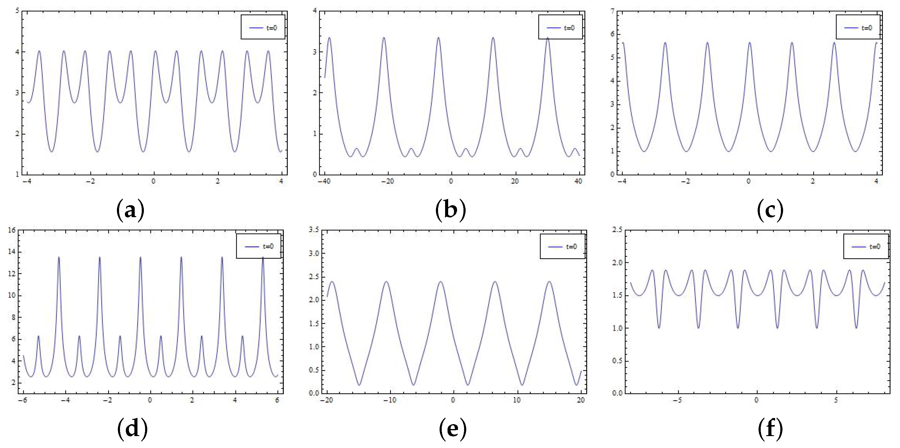
When $a=-1,b=0$, this solution reduces to the one for the nonlocal Sasa–Satsuma Equation (6). It can be seen that this solution is a double periodic wave. The periods in space and time are $\frac{\pi }{2{\lambda }_1^3}$ and $\frac{2\pi }{{\lambda }_1}$, respectively. The solution reaches the peak value and valley value

$$\begin{array}{cc}& |u^{\left(1\right)}{|}_{max}=max\{|\frac{4L_1}{L_2{\mathrm{e}}^{2{\mu }_1}+2ϵL_3{\mathrm{e}}^{-2{\mu }_1}}|,|\frac{4L_1}{L_2{\mathrm{e}}^{2{\mu }_1}-2ϵL_3{\mathrm{e}}^{-2{\mu }_1}}|\},\\ & |u^{\left(1\right)}{|}_{m\mathrm{i}n}=min\{|\frac{4L_1}{L_2{\mathrm{e}}^{2{\mu }_1}+2ϵL_3{\mathrm{e}}^{-2{\mu }_1}}|,|\frac{4L_1}{L_2{\mathrm{e}}^{2{\mu }_1}-2ϵL_3{\mathrm{e}}^{-2{\mu }_1}}|\}.\end{array}$$

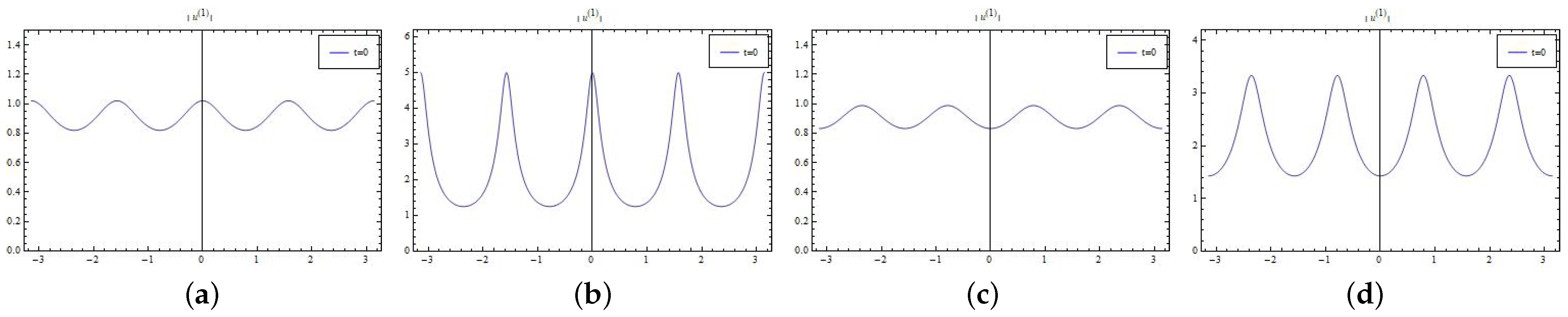
at the lines $t=\frac{2k\pi -8{\lambda }_{1}x}{32{\lambda }_1^3}(k\in N^{+})$. Taking $c_1=1,c_2=1+\mathrm{i},c_3=1,{\lambda }_1=1,$ we give the plot of the double periodic wave solution (see Figure 1) for the nonlocal gSS equation with $b=\frac{1}{5}$. For the focusing case, $\left(a\right)ϵ=1,a=-1$, $\left(b\right)ϵ=-1,a=1$; for the defocusing case, $\left(c\right)ϵ=1,a=1$, $\left(d\right)ϵ=-1,a=-1$. It can be seen from Figure 1 that only the peak and valley values of the solutions of the focusing case and the defocusing case are exchanged.

Case 2. Breather-like solution and breather solution

Set ${\lambda }_1={\alpha }_1+{\beta }_1\mathrm{i}$ $({\alpha }_1{\beta }_1\ne 0)$, and $c_2=0$. We obtain the solution

$$\begin{array}{cc}\hfill & u^{\left(1\right)}=\frac{4\mathrm{i}{c}_1{\lambda }_1{\lambda }_{1{,}_R}(ϵa|c_1{|}^2{c}_3^{*}{\lambda }_1^{*}{\mathrm{e}}^{2{\mu }_1}+ϵb^{*}{c}_1^{*2}{c}_3{\lambda }_{1{,}_R}{\mathrm{e}}^{2{\tilde{\mu }}_1^{*}}-\mathrm{i}{\lambda }_{1{,}_I}|c_3{|}^2{c}_3^{*}{\mathrm{e}}^{-2{\tilde{\mu }}_1^{*}})}{2ϵa|c_1{c}_3{\lambda }_1{|}^2+|c_1{|}^4(a^2|{\lambda }_1{|}^2-{|b|}^2{\lambda }_{1{,}_R}^2){\mathrm{e}}^{4\mathrm{i}{\mu }_{1,I}}+{|c_3|}^4{\lambda }_{1{,}_I}^2{\mathrm{e}}^{-4\mathrm{i}{\mu }_{1,I}}+ϵ{\lambda }_{1{,}_R}^2{L}_4},\end{array}$$

(21)

with $L_4=b{c}_1^2{c}_3^{*2}{\mathrm{e}}^{4{\mu }_{1,R}}+b^{*}{c}_1^{*2}{c}_3^2{\mathrm{e}}^{-4{\mu }_{1,R}}$. It is clear that when $b=0$, this solution is growing or decaying wave exponentially. Setting $c_1=1,c_3=1$, we give plots of the solution for the focusing nonlocal gSS equation with $ϵ=1,a=-1,b=\frac{1+\mathrm{i}}{5}$ and the defocusing nonlocal gSS equation with $ϵ=1,a=1,b=\frac{1+\mathrm{i}}{5}$ (see Figure 2 and Figure 3). In Figure 2 and Figure 3, we can see that the solution displays a periodic-like wave or breather traveling along the peak line. When ${\beta }_1^2<3{\alpha }_1^2$, this solution is periodic-like solution; when ${\beta }_1^2=3{\alpha }_1^2$, this solution is Kuznetsov–Ma (KM) breather-like solution. When ${\beta }_1^2>3{\alpha }_1^2$, this solution is a breather-like solution. It is worth noting that the nonlocal Sasa–Satsuma equation does not have a breather-like solution. It can also be seen from Figure 2 and Figure 3 that the shape and peak-position of solutions for the focusing and defocusing cases are different.

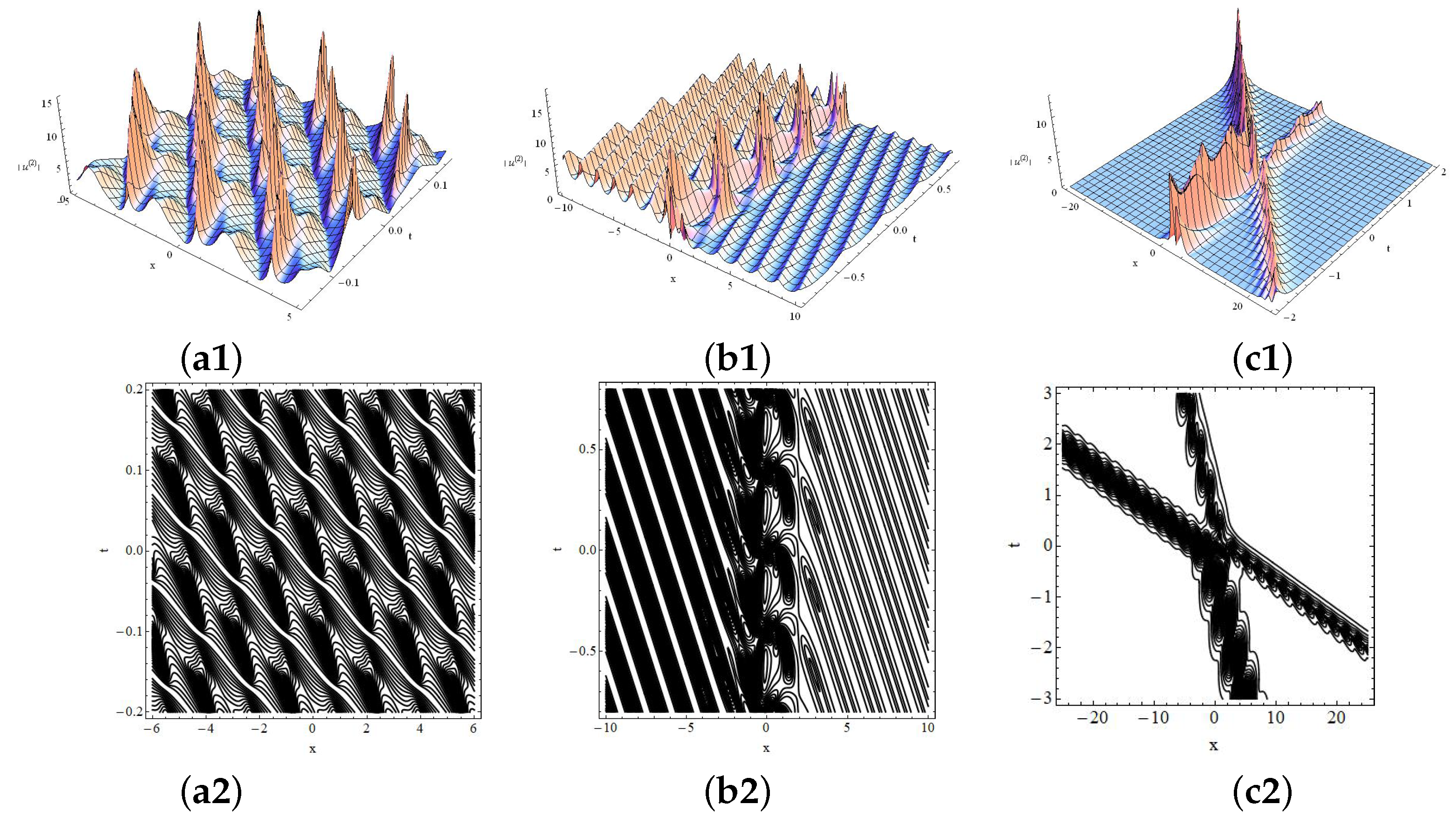
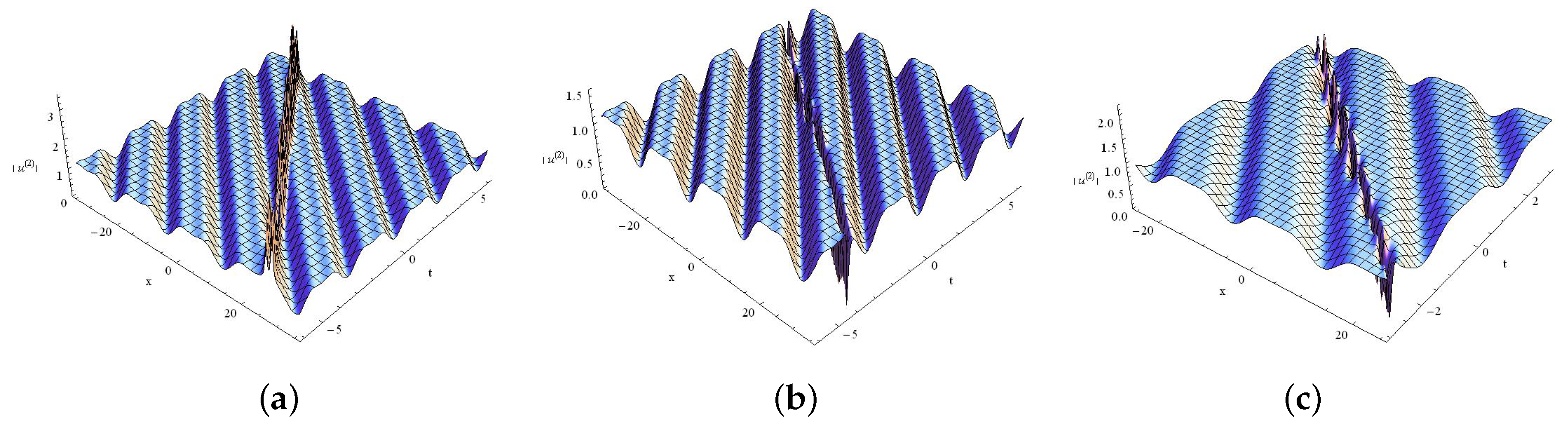
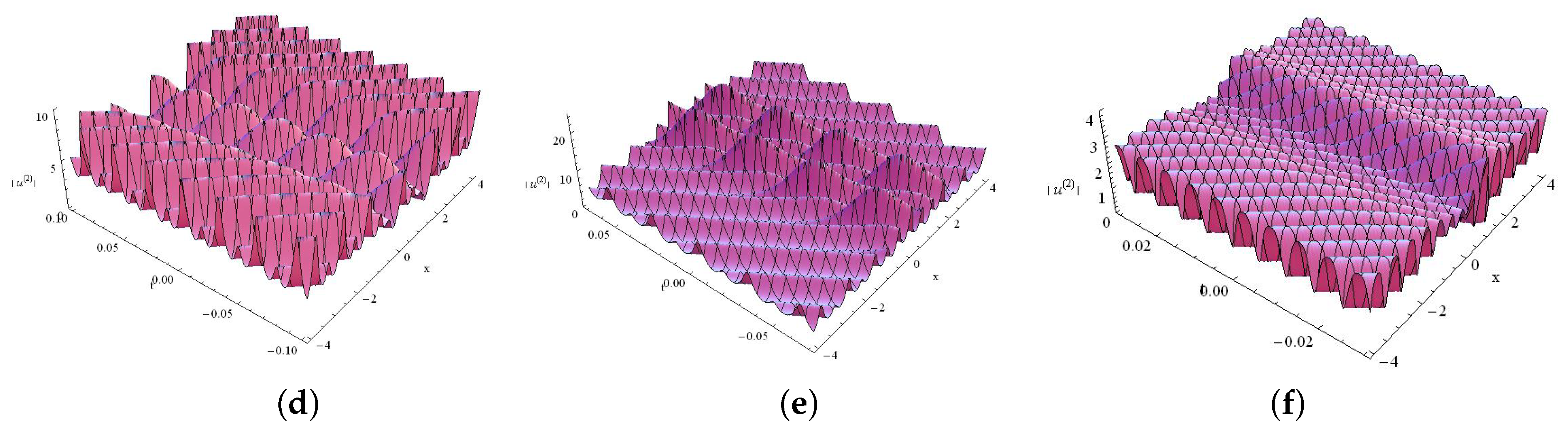
If $c_2\ne 0$, this solution is a breather solution. Because the expression of this solution is too complex, we omit its details. In Figure 4, we give the plot of the breather solution for the nonlocal gSS Equation (5) with $c_1=c_2=c_3=1$. For the focusing case with $ϵ=1,$ $a=-1,b=\frac{1}{5}$, when ${\lambda }_1=1+\frac{\mathrm{i}}{2}$, this solution is a periodic-like solution (see Figure 4a); when ${\lambda }_1=1+\sqrt{3}\mathrm{i}$, this solution is a KM-breather solution (see Figure 4b); when ${\lambda }_1=1+2\mathrm{i}$, this solution is a breather solution (see Figure 4c). For the defocusing case with $ϵ=1,a=1,b=\frac{1}{5}$, when ${\lambda }_1=1+\frac{\mathrm{i}}{2}$, this solution is a periodic-like solution (see Figure 4d); when ${\lambda }_1=1+\sqrt{3}\mathrm{i}$, this solution is a KM-breather solution (see Figure 4e); when ${\lambda }_1=1+2\mathrm{i}$, this solution is a breather solution (see Figure 4f). It can be seen from the figure that the crest position and crest value of breather solution for the focusing and defocusing cases have changed.

3.2. Interaction Solution of Double Periodic Wave and Breather

Let us give a two-fold DT. When $N=2$, the DT can be written as

$$\begin{array}{cc}\hfill & T^{\left(2\right)}=I-(|y_1\rangle ,|{\eta }_1\rangle ,|y_2\rangle ,|{\eta }_2\rangle ){\left(\begin{array}{cccc}{A}_1& B_1& C_1& D_1\\ {\tilde{B}}_1^{*}& A_1& {\tilde{D}}_1^{*}& {\tilde{C}}_1^{*}\\ {\tilde{C}}_1^{*}& D_1& A_2& D_2\\ {\tilde{D}}_1^{*}& C_1& {\tilde{D}}_2^{*}& A_2\end{array}\right)}^{-1}\left(\begin{array}{c}\frac{\langle y_1(-x,-t)|}{-{\lambda }_1^{*}-\lambda }\\ \frac{\langle {\eta }_1(-x,-t)|}{-{\lambda }_1^{*}-\lambda }\\ \frac{\langle y_2(-x,-t)|}{-{\lambda }_2^{*}-\lambda }\\ \frac{\langle {\eta }_2(-x,-t)|}{-{\lambda }_2^{*}-\lambda }\end{array}\right)\mathbf{J}\end{array}$$

(22)

where ${\tilde{C}}_1^{*}=C_1^{*}(-x,-t),{\tilde{D}}_k^{*}=D_k^{*}(-x,-t)(k=1,2)$, and

$$\begin{array}{cc}& A_k=\frac{\langle y_k(-x,-t)|J|y_k\rangle }{-{\lambda }_k^{*}-{\lambda }_k},B_1=\frac{\langle y_1(-x,-t)|J|{\eta }_1\rangle }{-2{\lambda }_1^{*}},C_1=\frac{\langle y_1(-x,-t)|J|y_2\rangle }{-{\lambda }_1^{*}-{\lambda }_2},D_k=\frac{\langle y_k(-x,-t)|J|{\eta }_2\rangle }{-{\lambda }_k^{*}-{\lambda }_2^{*}},\end{array}$$

and a 2-soliton solution of the focusing nonlocal gSS Equation (5) is given by

$$u^{\left(2\right)}=-2\mathrm{i}({\psi }_1^{\left(1\right)},{\tilde{\psi }}_2^{{\left(1\right)}^{*}},{\psi }_1^{\left(2\right)},{\tilde{\psi }}_2^{{\left(2\right)}^{*}}){\left(\begin{array}{cccc}{A}_1& B_1& C_1& D_1\\ {\tilde{B}}_1^{*}& A_1& {\tilde{D}}_1^{*}& {\tilde{C}}_1^{*}\\ {\tilde{C}}_1^{*}& D_1& A_2& D_2\\ {\tilde{D}}_1^{*}& C_1& {\tilde{D}}_2^{*}& A_2\end{array}\right)}^{-1}{({\tilde{\psi }}_3^{{\left(1\right)}^{*}},-ϵ{\psi }_3^{\left(1\right)},{\tilde{\psi }}_3^{{\left(2\right)}^{*}},-ϵ{\psi }_3^{\left(2\right)})}^T.$$

(23)

Let us discuss the focusing nonlocal gSS Equation (5) with $ϵ=1,a=-1,b=\frac{\mathrm{i}}{2}$. When ${\lambda }_1=1$, ${\lambda }_2=2$, we take parameters $c_1=1$, $c_2=0$, $c_3=1$, $c_4=1$, $c_5=0$ and $c_6=2\mathrm{i}$. This solution displays the interaction of two periodic waves (see Figure 5a); when ${\lambda }_1=1$, ${\lambda }_2=\frac{1}{2}+\frac{\sqrt{3}\mathrm{i}}{2}$, we take parameters $c_1=1$, $c_2=0$, $c_3=1$, $c_4=1$, $c_5=0$ and $c_6=1$. This solution describes the interaction of periodic wave and breather-like solutions (see Figure 5b); when ${\lambda }_1=1+\frac{\mathrm{i}}{3}$, ${\lambda }_2=\frac{1}{2}+\frac{\mathrm{i}}{2}$, we take parameters $c_1=1$, $c_2=0$, $c_3=1$, $c_4=1$, $c_5=0$ and $c_6=1$. This solution shows the interaction of breather and breather-like solitons (see Figure 5c). For the interaction of breather and breather-like solitons, we can analyze its asymptotic behavior as follows:

$$\begin{array}{c}\hfill u^{\left(2\right)}⟶\left\{\begin{array}{c}{u}_{11}^{-}+u_{21}^{-},t\to -\infty ,\hfill \\ u_{11}^{+}+u_{21}^{+},t\to +\infty ,\hfill \end{array}\right.\end{array}$$

(24)

where

$$\begin{array}{cc}& u_{11}^{-}=\frac{M_{11}}{M_{12}},u_{11}^{+}=\frac{M_{21}}{{\tilde{M}}_{12}^{*}},u_{21}^{-}=\frac{M_{31}}{M_{32}},u_{21}^{+}=\frac{M_{41}}{{\tilde{M}}_{32}^{*}},\\ & M_{11}=-\frac{187+204\mathrm{i}}{8692}{\mathrm{e}}^{2{\mu }_1}-\frac{2477-6735\mathrm{i}}{712744}{\mathrm{e}}^{-2{\tilde{\mu }}_1^{*}}+\frac{141-63\mathrm{i}}{44944}{\mathrm{e}}^{2{\tilde{\mu }}_1^{*}},\\ & M_{12}=\frac{85\mathrm{i}}{17384}-\frac{45{\mathrm{e}}^{-2({\mu }_1-{\tilde{\mu }}_1^{*})}}{179776}+\frac{132264+128927\mathrm{i}}{755508640}{\mathrm{e}}^{-2({\mu }_1+{\tilde{\mu }}_1^{*})}+\frac{22689+14256\mathrm{i}}{537920}{\mathrm{e}}^{2({\mu }_1-{\tilde{\mu }}_1^{*})}+\frac{11453112+1559609\mathrm{i}}{3022034560}{\mathrm{e}}^{2({\mu }_1+{\tilde{\mu }}_1^{*})},\\ & M_{21}=\frac{34-63\mathrm{i}}{8692}{\mathrm{e}}^{2{\mu }_1}-\frac{3189+1065\mathrm{i}}{178186}{\mathrm{e}}^{-2{\mu }_1}-\frac{1021+897\mathrm{i}}{921352}{\mathrm{e}}^{-2{\tilde{\mu }}_1^{*}}+\frac{127749-1047\mathrm{i}}{1425488}{\mathrm{e}}^{2{\tilde{\mu }}_1^{*}},\\ & M_{31}=-\frac{3+14\mathrm{i}}{17384}{\mathrm{e}}^{2{\mu }_2}-\frac{1307+5449\mathrm{i}}{890930}{\mathrm{e}}^{-2{\mu }_2}+\frac{277-541\mathrm{i}}{1842704}{\mathrm{e}}^{-2{\tilde{\mu }}_2^{*}}+\frac{154997+126291\mathrm{i}}{1425880}{\mathrm{e}}^{2{\tilde{\mu }}_2^{*}},\\ & M_{32}=\frac{17\mathrm{i}}{17384}+\frac{5{\mathrm{e}}^{2({\mu }_2-{\tilde{\mu }}_2^{*})}}{179776}-\frac{107976+149857\mathrm{i}}{755508640}{\mathrm{e}}^{-2({\mu }_2+{\tilde{\mu }}_2^{*})}-\frac{2521+1584\mathrm{i}}{537920}{\mathrm{e}}^{-2({\mu }_2-{\tilde{\mu }}_2^{*})}-\frac{899448+483439\mathrm{i}}{3022034560}{\mathrm{e}}^{2({\mu }_2+{\tilde{\mu }}_2^{*})},\\ & M_{41}=-\frac{187+204\mathrm{i}}{86920}{\mathrm{e}}^{2{\mu }_2}+\frac{23+\mathrm{i}}{89888}{\mathrm{e}}^{2{\tilde{\mu }}_2^{*}}+\frac{12599+9937\mathrm{i}}{7127440}{\mathrm{e}}^{-2{\tilde{\mu }}_2^{*}}.\end{array}$$

4. Soliton, Breather, and Periodic Wave Solutions for Equation (5) with the Nonzero Seed Solution

For the nonzero seed solution $u=\gamma$ ($\gamma \ne 0$, $\gamma$ is a real constant), solving spectral problem (8) at $\lambda ={\lambda }_j$, we obtain the the eigenfunction

$$\begin{array}{cc}\hfill & {\mathsf{\Psi }}_j={({\psi }_1^{\left(j\right)},{\psi }_2^{\left(j\right)},{\psi }_3^{\left(j\right)})}^T,{\psi }_1^{\left(j\right)}=d_{j1}{\mathrm{e}}^{{\chi }_j}+d_{j2}{\mathrm{e}}^{-{\chi }_j}+(a+b^{*})d_{j3}{\mathrm{e}}^{{\xi }_j},\\ \hfill & {\psi }_2^{\left(j\right)}=ϵ(d_{j1}{\mathrm{e}}^{{\chi }_j}+d_{j2}{\mathrm{e}}^{-{\chi }_j}-(a+b)d_{j3}{\mathrm{e}}^{{\xi }_j}),{\psi }_3^{\left(j\right)}=\frac{1}{\gamma }(d_{j1}({\kappa }_j-\mathrm{i}{\lambda }_j){\mathrm{e}}^{{\chi }_j}-d_{j2}({\kappa }_j+\mathrm{i}{\lambda }_j){\mathrm{e}}^{-{\chi }_j}),\\ \hfill & {\chi }_j={\kappa }_j(x+2{\omega }_{j}t),{\xi }_j=\mathrm{i}{\lambda }_j(x+4{\lambda }_j^{2}t),{\kappa }_j=\sqrt{ϵ{\gamma }^2(2a+b+b^{*})-{\lambda }_j^2},{\omega }_j=ϵ{\gamma }^2(2a+b+b^{*})+2{\lambda }_j^2,\end{array}$$

(25)

where $d_{j1},d_{j2},d_{j3}$ are complex constants.

4.1. Soliton, Breather, and Periodic Wave Solutions

By one-fold DT (18), we obtain the following soliton solution of the nonlocal gSS Equation (5):

$$\begin{array}{c}\hfill u^{\left(1\right)}=\gamma +\frac{2\mathrm{i}(A_1(ϵ{\tilde{\psi }}_2^{{\left(1\right)}^{*}}{\psi }_3^{\left(1\right)}-{\psi }_1^{\left(1\right)}{\tilde{\psi }}_3^{{\left(1\right)}^{*}})-ϵB_1{\psi }_1^{\left(1\right)}{\psi }_3^{\left(1\right)}+{\tilde{B}}_1^{*}{\tilde{\psi }}_2^{{\left(1\right)}^{*}}{\tilde{\psi }}_3^{{\left(1\right)}^{*}})}{A_1^2-B_1{\tilde{B}}_1^{*}},\end{array}$$

(26)

where $A_1,B_1$ are defined by (19), and ${\psi }_k^{\left(1\right)}(k=1,2,3)$ are given in (25). In the following, we set $\gamma =1$, $d_{11}=1$, ${\lambda }_1={\alpha }_1$ in the formula of the solution.

Case 1.

$(2a+b+b^{*}){\gamma }^2ϵ-{\alpha }_1^2>0$

In this case, the solution of the nonlocal gSS Equation (26) can be written as

$$\begin{array}{cc}\hfill & u^{\left(1\right)}=1-4\mathrm{i}ϵ{\alpha }_1\frac{(a^2-{|b|}^2)H_1+2{\kappa }_1(a+b^{*})(|d_{12}{|}^2-1)((d_{13}^{*}+d_{12}^{*}{d}_3){\mathrm{e}}^{{\chi }_1-{\xi }_1}+(d_{13}+d_{12}{d}_{13}^{*}){\mathrm{e}}^{-{\chi }_1-{\xi }_1})}{(a^2-{|b|}^2)H_2+4ϵ{\kappa }_1^2(|d_{12}{{|}^2-1)}^2{\mathrm{e}}^{-2{\xi }_1}},\end{array}$$

(27)

with $p=2a+b+b^{*}$ and

$$\begin{array}{cc}& H_1={(d_{13}^{*}+d_{12}^{*}{d}_{13})}^2({\kappa }_1-{\alpha }_1\mathrm{i}){\mathrm{e}}^{2{\chi }_1}-{(d_{13}+d_{12}{d}_{13}^{*})}^2({\kappa }_1+{\alpha }_1\mathrm{i}){\mathrm{e}}^{-2{\chi }_1}-2\mathrm{i}{\alpha }_1{|d_{13}+d_{12}{d}_{13}^{*}|}^2,\\ & H_2={(d_{13}^{*}+d_{12}^{*}{d}_{13})}^2(p-ϵ{({\kappa }_1-{\alpha }_1\mathrm{i})}^2){\mathrm{e}}^{2{\chi }_1}+{(d_{13}+d_{12}{d}_{13}^{*})}^2(p-ϵ{({\kappa }_1+{\alpha }_1\mathrm{i})}^2){\mathrm{e}}^{-2{\chi }_1}+4p{|d_{13}+d_{12}{d}_{13}^{*}|}^2.\end{array}$$

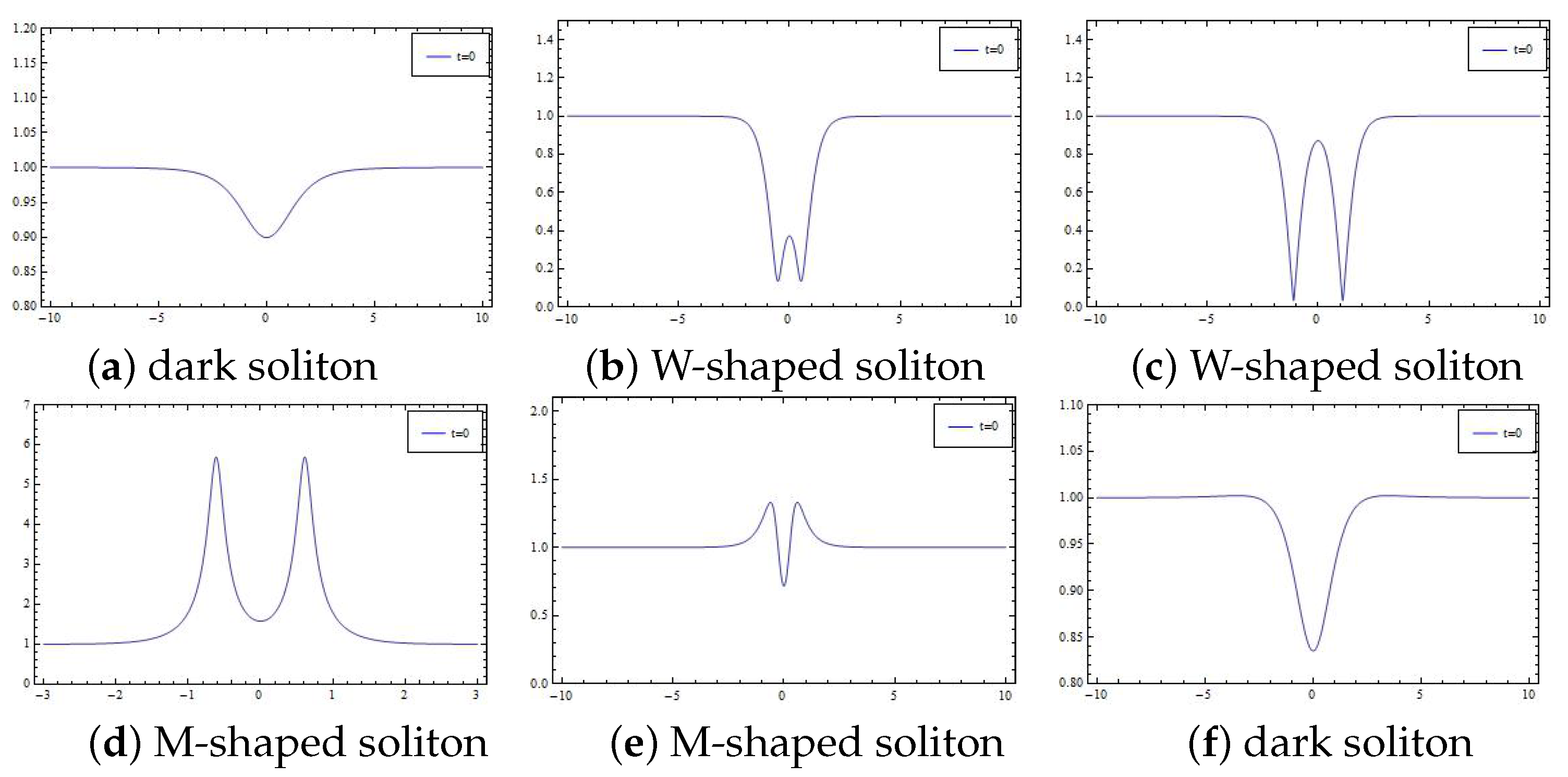
If $|d_{12}|=1$, this solution is the hump-type soliton, where the wave crest and wave trough are located on straight lines. Because the expression is too complex, we take parameters as $d_{12}=\mathrm{i}$, $d_{13}=2$. For the defocusing case with $ϵ=1,a=1,b=\frac{1}{5}$, we obtain dark soliton, W-shaped soliton, or M-shaped soliton solutions (see Figure 6). Figure 6 shows the progress of a dark soliton becoming a W-shaped soliton and the progress of an M-shaped soliton becoming a dark soliton. When ${\alpha }_1>0$, when the value of ${\alpha }_1$ decreases, the dark soliton becomes a W-shaped soliton; When ${\alpha }_1<0$, when the value of ${\alpha }_1$ decreases, the M-shaped soliton becomes a dark soliton. For $(2a+b+b^{*}){\gamma }^2ϵ-{\alpha }_1^2=\frac{12}{5}-{\alpha }_1^2>0$, when ${\alpha }_1=\frac{3}{2}$, the trough value $0.899$ of this dark soliton is taken at the line $t=-\frac{15x}{207}$; when ${\alpha }_1=\frac{1}{2}$, trough value $0.134$ and peak value $0.372$ of this W-shaped soliton are taken at lines

$$\begin{array}{c}\hfill t=-\frac{5x}{29}+\frac{5\sqrt{5}}{29\sqrt{43}}ln\left(\frac{\sqrt{235671}-60\pm \sqrt{3(69437-40\sqrt{235671})}}{12\sqrt{215}}\right),\mathit{and}t=-\frac{5x}{29},\end{array}$$

respectively; when ${\alpha }_1=\frac{1}{10}$, trough value $0.032$ and peak value $0.871$ of this W-shaped soliton are taken at lines

$$\begin{array}{c}\hfill t=-\frac{25x}{121}+\frac{5\sqrt{5}}{121\sqrt{239}}ln\left(\frac{\sqrt{204775215}-60\pm \sqrt{15(13594561-8\sqrt{204775215})}}{60\sqrt{239}}\right)\mathit{and}t=-\frac{25x}{121},\end{array}$$

respectively; when ${\alpha }_1=-\frac{1}{2}$, trough value $1.580$ and peak value $5.690$ of this M-shaped soliton are taken at lines

$$\begin{array}{c}\hfill t=-\frac{5x}{29}+\frac{5\sqrt{5}}{29\sqrt{43}}ln\left(\frac{\sqrt{235671}+60\pm \sqrt{3(69437-40\sqrt{235671})}}{12\sqrt{215}}\right)\mathit{and}t=-\frac{5x}{29},\end{array}$$

respectively; when ${\alpha }_1=-\frac{7}{6}$, trough value $0.716$ and peak value $1.330$ of this M-shaped soliton are taken at lines

$$\begin{array}{c}\hfill t=-\frac{45x}{461}\mathit{and}t=-\frac{45x}{461}+\frac{13\sqrt{5}}{461\sqrt{187}}ln\left(\frac{61\sqrt{8079}+8820\pm \sqrt{48478119+1076040\sqrt{8079})}}{252\sqrt{935}}\right),\end{array}$$

respectively; when ${\alpha }_1=-\frac{3}{2}$, trough value $0.835$ and peak value $1.002$ of this M-shaped soliton are taken at lines

$$\begin{array}{c}\hfill t=-\frac{15x}{207}\mathit{and}t=-\frac{15x}{207}+\frac{5\sqrt{15}}{207}ln\left(\frac{\sqrt{3151}+60\pm \sqrt{6511+120\sqrt{3151}}}{4\sqrt{15}}\right),\end{array}$$

respectively. For the focusing case with $a=1,ϵ=-1$, existence of this hump-type solution is related to the value ofb, e.g., if we take $b=\frac{1}{5}$, there is not such a hump-type solution; however, if we take $b=2$, there is such a hump-type soliton, which is similar to the case described by Figure 6.

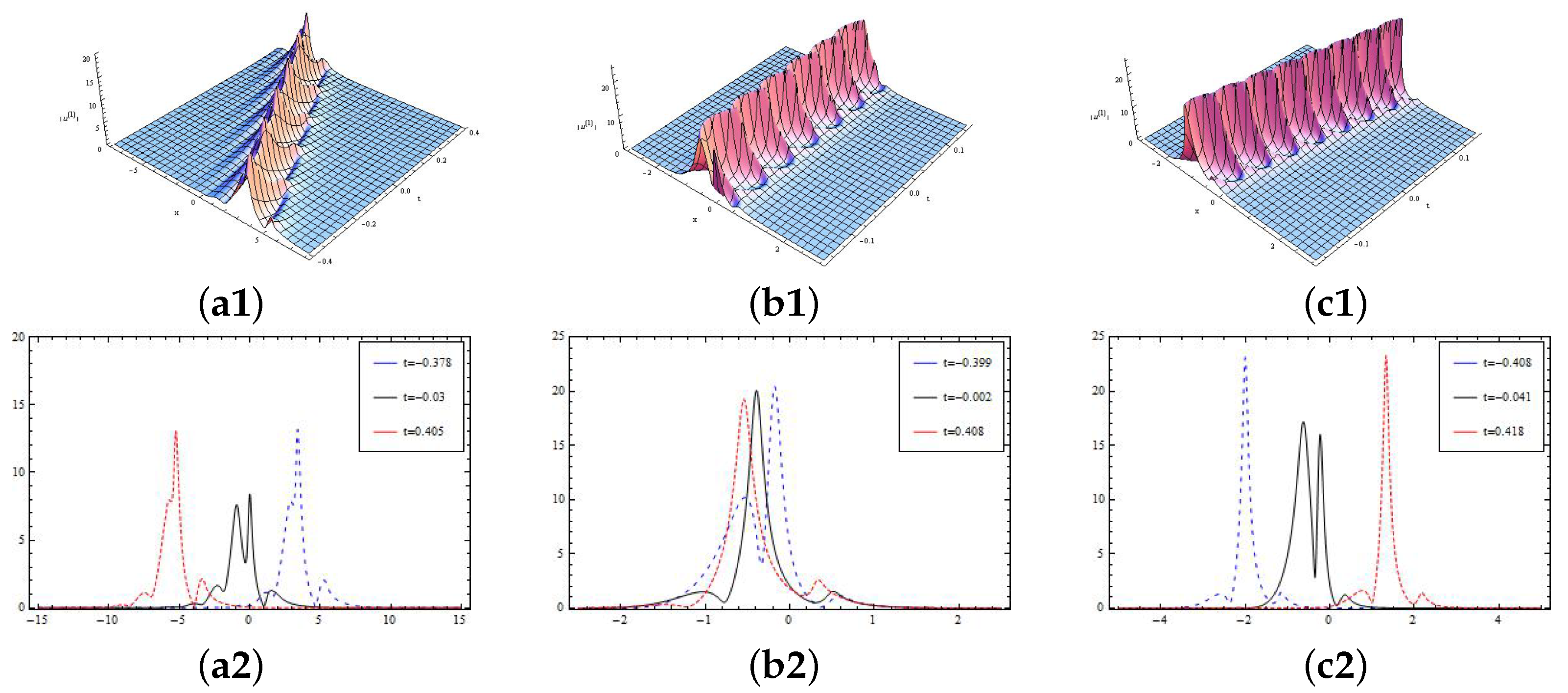
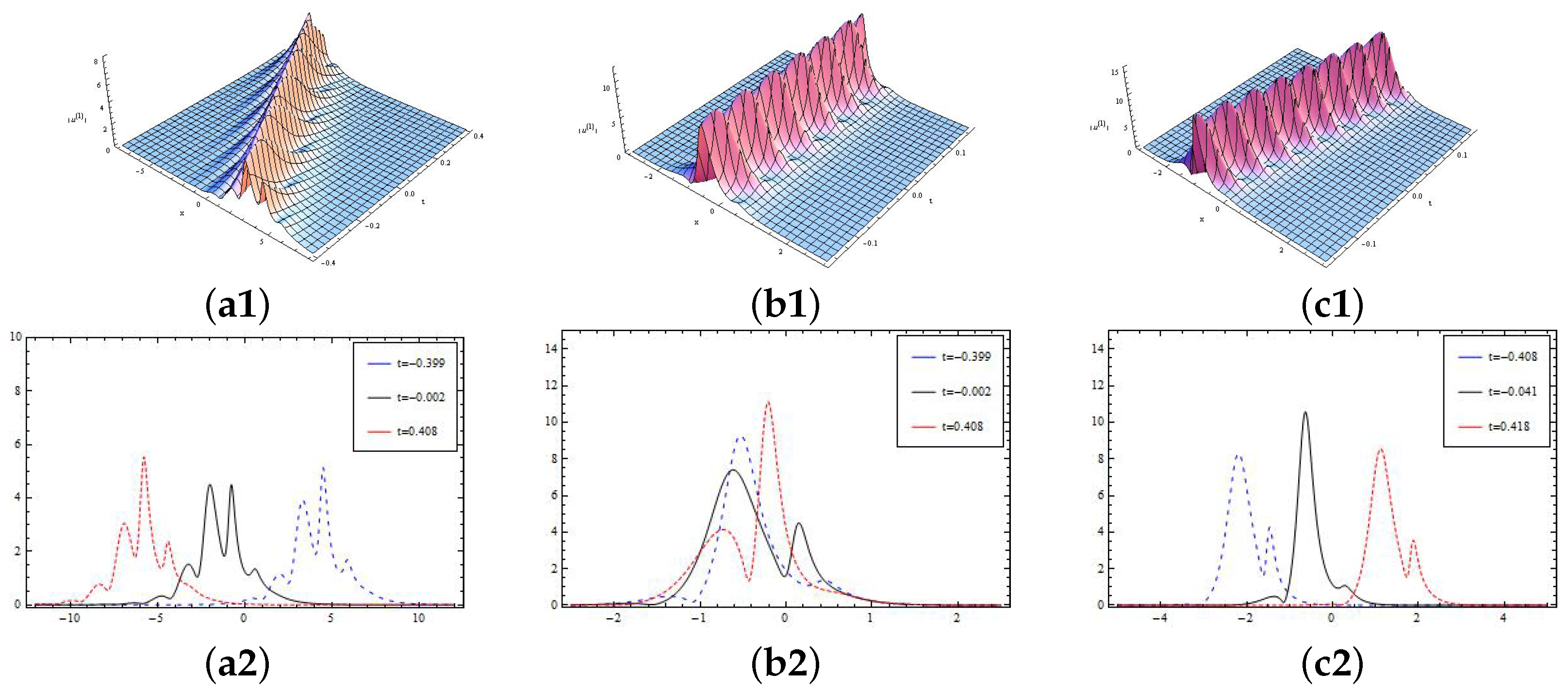
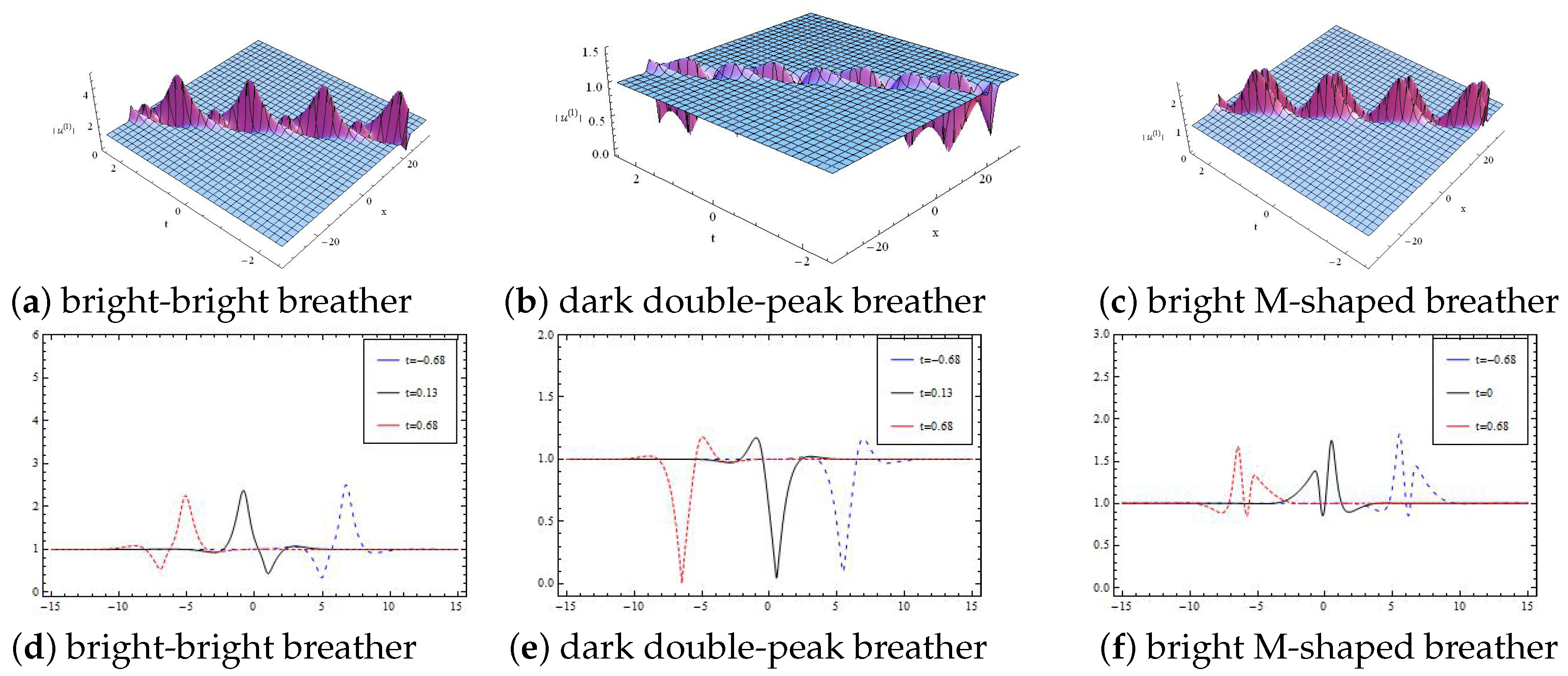
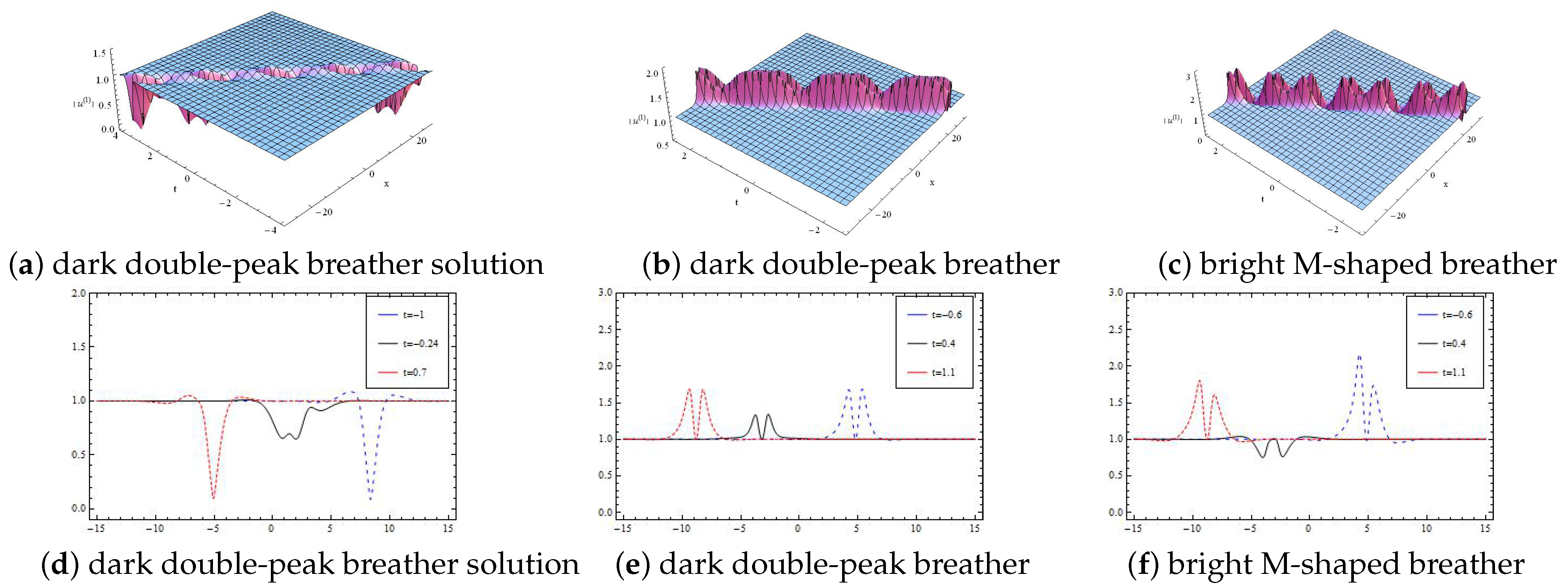
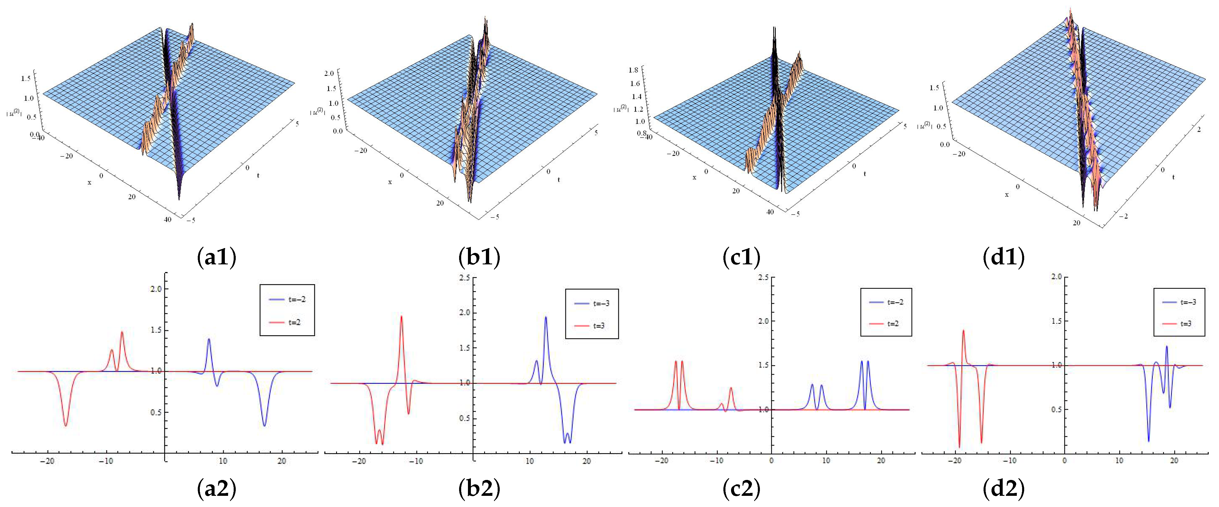
If $|d_{12}|\ne 1$, this solution is a breather solution. Here we discuss breather solutions of the defocusing nonlocal gSS Equation (5) with $ϵ=1,a=1,b=\frac{1}{5}$ and the focusing nonlocal gSS Equation (5) with $ϵ=1,a=-1,b=2$. Taking $d_{12}=0$, ${\alpha }_1=1$, for the defocusing case, when $d_{13}=1$, this solution is a bright-bright breather solution (see Figure 7a,d); when $d_{13}=3$, this solution is a dark double-peak breather solution (see Figure 7b,e); when $d_{13}=3\mathrm{i}$, this solution is a bright M-shaped breather solution (see Figure 7c,f). For the focusing case, when $d_{13}=1$, this solution is a dark double-peak breather solution (see Figure 8a,d); when $d_{13}=\mathrm{i}$, this solution is an M-shaped double-peak-breather solution (see Figure 8b,e); when $d_{13}=3\mathrm{i}$, this solution is an M-shaped double-peak-breather solution (see Figure 8c,f).

Case 2.

$(2a+b+b^{*}){\gamma }^2ϵ-{\alpha }_1^2<0$

In this case, the solution of the nonlocal gSS Equation (5) can be written as

$$\begin{array}{cc}\hfill & u^{\left(1\right)}=1-4\mathrm{i}ϵ{\alpha }_1\frac{(a^2-{|b|}^2)H_3+4\mathrm{i}{\kappa }_1(a+b^{*})d_{12,I}(2d_{13,R}{\mathrm{e}}^{-{\chi }_1+{\xi }_1}+(d_{12}^{*}{d}_{13}+d_{12}{d}_{13}^{*}){\mathrm{e}}^{-{\chi }_1-{\xi }_1})}{(a^2-{|b|}^2)H_4-4ϵ{\kappa }_1^2{d}_{12,I}^2{\mathrm{e}}^{-2{\xi }_1}},\end{array}$$

(28)

with

$$\begin{array}{cc}& H_3=4d_{13,R}^2({\kappa }_1-{\alpha }_1\mathrm{i}){\mathrm{e}}^{2{\chi }_1}-{(d_{12}^{*}{d}_{13}+d_{12}{d}_{13}^{*})}^2({\kappa }_1+{\alpha }_1\mathrm{i}){\mathrm{e}}^{-2{\chi }_1}-4\mathrm{i}{\alpha }_1{d}_{3,R}(d_{12}{d}_{13}^{*}+d_{12}^{*}{d}_{13}),\\ & H_4=4d_{13,R}^2(p-ϵ{({\kappa }_1-{\alpha }_1\mathrm{i})}^2){\mathrm{e}}^{2{\chi }_1}+{(d_{12}{d}_{13}^{*}+d_{12}^{*}{d}_{13})}^2(p-ϵ{({\kappa }_1+{\alpha }_1\mathrm{i})}^2){\mathrm{e}}^{-2{\chi }_1}+8p{d}_{13,R}(d_{12}{d}_{13}^{*}+d_{12}^{*}{d}_{13}).\end{array}$$

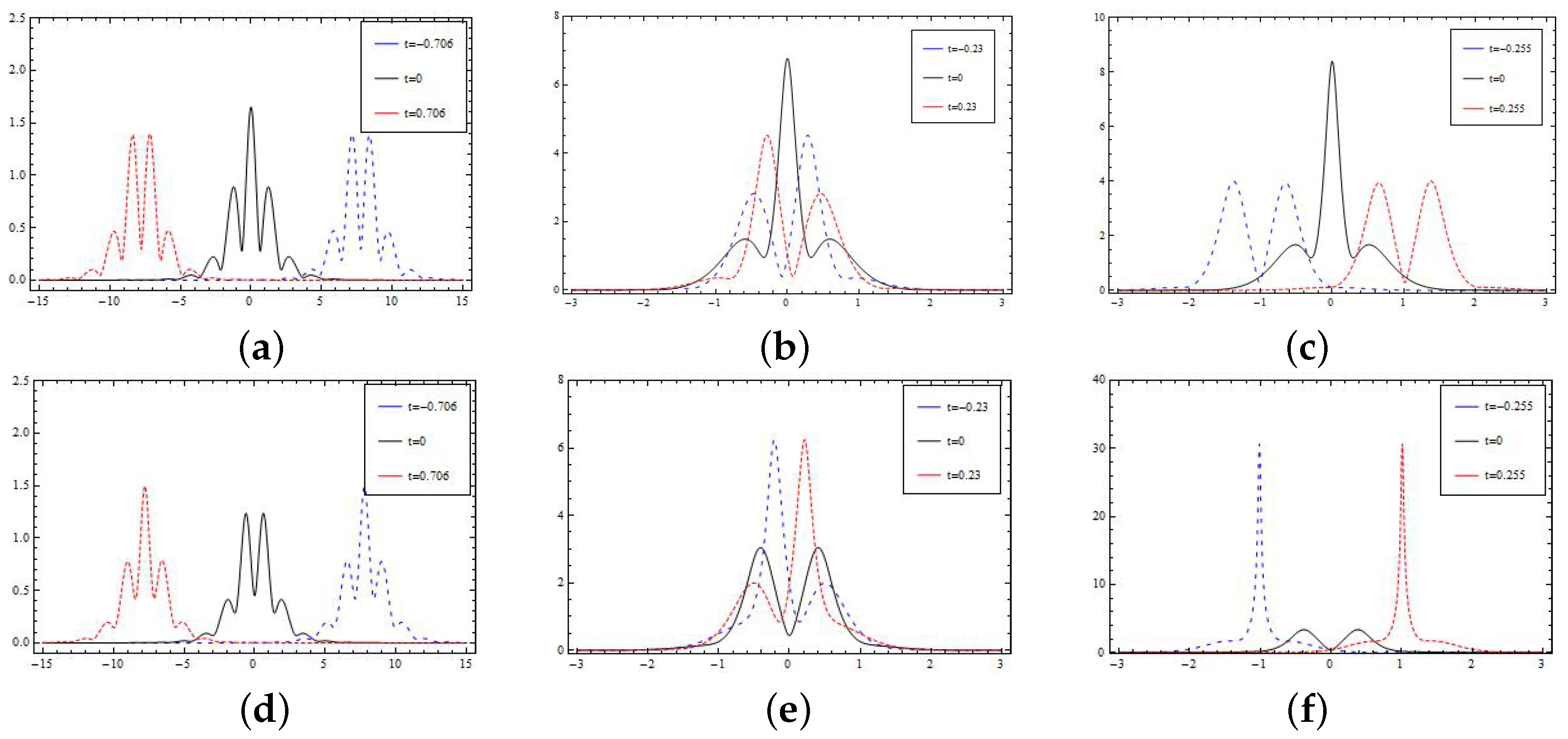
If $d_{12}$ is a real number, or $d_{13}$ is a pure imaginary number, or $d_{12}$ is a pure imaginary number and $d_{13}$ is a real number, $\mathrm{i}.e.,$ $d_{12,I}=0$, or $d_{13,R}=0$, or $d_{12}{d}_{13}^{*}+d_{12}^{*}{d}_{13}=0$ $(d_{12,I}·d_{13,R}\ne 0)$, this solution is a periodic wave-type solution. When taking $d_{12}=\mathrm{i}$, $d_{13}=2$, $b=\frac{1}{5}$, for the focusing Equation (6) with $ϵ=1,a=-1$, this solution is an M-shaped periodic wave and W-shaped periodic wave with ${\alpha }_1=2$ and ${\alpha }_1=-2$, respectively (see Figure 9a,b); whereas for the defocusing Equation (6) with $ϵ=1,a=1$, this solution is a W-shaped periodic wave and classical periodic wave with ${\alpha }_1=2$ and ${\alpha }_1=-2$, respectively (see Figure 9d,e). When taking $d_{12}=1$, $d_{13}=2$, $b=\frac{1}{5}$, for the focusing Equation (6) with $ϵ=1,a=-1$, this solution is a classical periodic wave with ${\alpha }_1=2$ (see Figure 9c); whereas for the defocusing Equation (6) with $ϵ=1,a=1$, this solution is an M-shaped periodic wave with ${\alpha }_1=2$ (see Figure 9f).

When $d_{12,I}\ne 0$, $d_{13,R}\ne 0$, and $d_{12}{d}_{13}^{*}+d_{12}^{*}{d}_{13}\ne 0$, this solution is breather-periodic wave solution. In Figure 10, taking $ϵ=1,b=\frac{1}{5}$, for the focusing case with $a=-1,{\alpha }_1=\frac{1}{2}$, this solution is a double-peak breather-periodic wave solution with $d_{12}=1+\frac{\mathrm{i}}{2},$ $d_{13}=2$ or $d_{12}=\mathrm{i},$ $d_{13}=1+\frac{\mathrm{i}}{2}$ (see Figure 10a–d); for the defocusing case with $a=-1,{\alpha }_1=3$: this solution is breather-periodic wave solution with $d_{12}=\mathrm{i},d_{13}=1+\frac{\mathrm{i}}{2}$ or $d_{12}=1+\frac{\mathrm{i}}{2},d_{13}=2$ (see Figure 10e,f).

Case 3.

$\mathrm{Im}[(2a+b+b^{*}){\gamma }^2ϵ-{\lambda }_1^2]\ne 0$

When ${\lambda }_1$ is a complex number, the solution (26) of the nonlocal gSS equation is a breather-type solution. Because its expression is too complicated, we omit it. Take the plot of Figure 11 as an example. Setting $d_{11}=1,d_{12}=0,d_{13}=3$, and ${\lambda }_1=1+\frac{\mathrm{i}}{2}$, the solution of the focusing nonlocal gSS equation with $ϵ=1,a=-1,b=\frac{1}{5}$ is a double-peak breather solution (see Figure 11a,b); the solution of the defocusing nonlocal gSS equation with $ϵ=1,a=1,b=\frac{1}{5}$ is a bright-bright breather solution (see Figure 11c,d).

4.2. Interaction Solution of Hump–Soliton, Breather, and Periodic Wave Solutions

By two-fold DT (22), we obtain the interaction solution of the focusing nonlocal gSS Equation (5)

$$\begin{array}{c}\hfill u^{\left(2\right)}=1-2\mathrm{i}({\psi }_1^{\left(1\right)},{\tilde{\psi }}_2^{{\left(1\right)}^{*}},{\psi }_1^{\left(2\right)},{\tilde{\psi }}_2^{{\left(2\right)}^{*}}){\left(\begin{array}{cccc}{A}_1& B_1& C_1& D_1\\ {\tilde{B}}_1^{*}& A_1& {\tilde{D}}_1^{*}& {\tilde{C}}_1^{*}\\ {\tilde{C}}_1^{*}& D_1& A_2& D_2\\ {\tilde{D}}_1^{*}& C_1& {\tilde{D}}_2^{*}& A_2\end{array}\right)}^{-1}{({\tilde{\psi }}_3^{{\left(1\right)}^{*}},-ϵ{\psi }_3^{\left(1\right)},{\tilde{\psi }}_3^{{\left(2\right)}^{*}},-ϵ{\psi }_3^{\left(2\right)})}^T\end{array}$$

(29)

where $A_k,B_1,C_1,D_k$ are defined by (22).

Let us discuss the focusing nonlocal gSS Equation (5) with $ϵ=1,a=-1,b=2$. When ${\lambda }_1$ and ${\lambda }_2$ are real numbers, we take parameters $d_{11}=1$, $d_{12}=0$, $d_{13}=2$, $d_{21}=1$, $d_{22}=\mathrm{i}$, $d_{23}=2$; this solution displays the collision of breather with hump solitons or periodic waves (see Figure 10). For the collision of a breather and hump soliton, where ${\lambda }_1$ and ${\lambda }_2$ are real numbers and $(2a+b+b^{*}){\gamma }^2ϵ-{\alpha }_j^2>0$, we analyze its asymptotic behavior as follows:

$$\begin{array}{c}\hfill u^{\left(2\right)}⟶\left\{\begin{array}{c}{u}_{21}^{-}+u_{22}^{-},t\to -\infty ,\hfill \\ u_{21}^{+}+u_{22}^{+},t\to +\infty ,\hfill \end{array}\right.\end{array}$$

(30)

where

$$\begin{array}{cc}& u_{21}^{-}=1-\frac{M_{51}}{M_{52}},u_{22}^{-}=1-\frac{4({\alpha }_1^2-{\alpha }_2^2)(2-{\alpha }_2^2)({\kappa }_1+{\alpha }_1\mathrm{i})}{4({\alpha }_1^2-{\alpha }_2^2)({\kappa }_1+{\alpha }_1\mathrm{i})-{\alpha }_2{P}_1{\mathrm{e}}^{-2{\chi }_2}+{\alpha }_2{P}_2{\mathrm{e}}^{2{\chi }_2}},\\ & u_{21}^{+}=1-\frac{M_{61}}{{\tilde{M}}_{52}^{*}},u_{22}^{+}=1-\frac{4({\alpha }_1^2-{\alpha }_2^2)(2-{\alpha }_2^2)({\kappa }_1-{\alpha }_1\mathrm{i})}{4({\alpha }_1^2-{\alpha }_2^2)({\kappa }_1-{\alpha }_1\mathrm{i})-{\alpha }_2{P}_1^{*}{\mathrm{e}}^{2{\chi }_2}+{\alpha }_2{P}_2^{*}{\mathrm{e}}^{-2{\chi }_2}},\\ & M_{51}=2({\alpha }_1+{\alpha }_2)((2-{\alpha }_1^{*})({\kappa }_2+{\alpha }_2\mathrm{i})({\alpha }_1+{\alpha }_2+12({\alpha }_1-{\alpha }_2){\mathrm{e}}^{2{\xi }_1})-2{\alpha }_1(P_3{\mathrm{e}}^{{\chi }_1-{\xi }_1}+P_4{\mathrm{e}}^{{\chi }_1+{\xi }_1})),\\ & M_{52}=({\kappa }_2+{\alpha }_2\mathrm{i})((2-{\alpha }_2^2){({\alpha }_1+{\alpha }_2)}^2+24({\alpha }_1^2-{\alpha }_2^2){\mathrm{e}}^{2{\xi }_1})-6\mathrm{i}{\alpha }_1(P_1{\mathrm{e}}^{2({\chi }_1-{\xi }_1)}+P_2^{*}{\mathrm{e}}^{2({\chi }_1+{\xi }_1)}),\\ & M_{61}=2({\alpha }_1+{\alpha }_2)((2-{\alpha }_1^{*})({\kappa }_2-{\alpha }_2\mathrm{i})({\alpha }_1+{\alpha }_2+12({\alpha }_1-{\alpha }_2){\mathrm{e}}^{2{\xi }_1})+2{\alpha }_1(P_4^{*}{\mathrm{e}}^{{\chi }_1-{\xi }_1}+P_3^{*}{\mathrm{e}}^{{\chi }_1+{\xi }_1})),\end{array}$$

with ${\tilde{M}}_{kj}^{*}=M_{kj}^{*}(-x,-t)$, ${\kappa }_j(j=1,2)$ given by Equation (25), and

$$\begin{array}{ccc}& & P_1={({\alpha }_1-{\alpha }_2)}^2(2+{\alpha }_1{\alpha }_2-{\kappa }_1{\kappa }_2)-2(4-{\alpha }_1^2-{\alpha }_2^2-2{\kappa }_1{\kappa }_2)\hfill \\ & & -\mathrm{i}({\alpha }_1-{\alpha }_2)((4+{\alpha }_1{\alpha }_2-{\alpha }_2^2){\kappa }_1-(4+{\alpha }_1{\alpha }_2-{\alpha }_1^2){\kappa }_2),\hfill \\ & & P_2={({\alpha }_1-{\alpha }_2)}^2(2+{\alpha }_1{\alpha }_2+{\kappa }_1{\kappa }_2)-2(4-{\alpha }_1^2-{\alpha }_2^2+2{\kappa }_1{\kappa }_2)\hfill \\ & & -\mathrm{i}({\alpha }_1-{\alpha }_2)((4+{\alpha }_1{\alpha }_2-{\alpha }_2^2){\kappa }_1+(4+{\alpha }_1{\alpha }_2-{\alpha }_1^2){\kappa }_2),\hfill \\ & & P_3=(2-{\alpha }_2^2){\kappa }_1-(2-{\alpha }_1^2){\kappa }_2-\mathrm{i}{\alpha }_2(2-{\alpha }_1^2-{\kappa }_1{\kappa }_2),\hfill \\ & & P_4=(2-{\alpha }_2^2){\kappa }_1+(2-{\alpha }_1^2){\kappa }_2+\mathrm{i}{\alpha }_2(2-{\alpha }_1^2+{\kappa }_1{\kappa }_2).\hfill \end{array}$$

In Figure 12, when ${\lambda }_1=\frac{1}{3}$, ${\lambda }_2=1$, this solution shows the interaction of an M-shaped double-peak-breather and dark soliton; when ${\lambda }_1=\frac{1}{3}$, ${\lambda }_2=\frac{1}{2}$, this solution displays the interaction of an M-shaped double-peak-breather and W-shaped soliton; when ${\lambda }_1=\frac{1}{3}$, ${\lambda }_2=-1$, this solution shows the interaction of an M-shaped double-peak-breather and M-shaped soliton. If ${\lambda }_1=1+\frac{\mathrm{i}}{2}$, ${\lambda }_2=1$, this solution displays the interaction of a double-peak-breather and a dark soliton. If ${\lambda }_1=\frac{1}{3}$, ${\lambda }_2=-3$, this solution describes the interaction of an M-shaped double-peak-breather and an M-shaped periodic wave (see Figure 13a). If ${\lambda }_1=1$, ${\lambda }_2=-3$, this solution shows the interaction of a dark-breather and an M-shaped periodic wave (see Figure 13b. If ${\lambda }_1=1+\frac{\mathrm{i}}{5}$, ${\lambda }_2=-3$, this solution shows the interaction of a double-peak breather and anM-shaped periodic wave (see Figure 13c).

For the nonlocal defocusing gSS equation with $ϵ=1,a=1,b=\frac{1}{5}$, taking $d_{11}=1$, $d_{12}=0,d_{13}=3,d_{21}=1,d_{22}=\mathrm{i},d_{23}=2$, ${\lambda }_1=\frac{1}{3},{\lambda }_2=3$, this solution describes the interaction of a bright-bright breather and a W-shaped periodic wave (see Figure 13d); taking $d_{11}=1,d_{12}=0,d_{13}=3\mathrm{i},d_{21}=1,d_{22}=\mathrm{i},d_{23}=2$, ${\lambda }_1=\frac{1}{3},{\lambda }_2=3$, this solution describes the interaction of a double-peak breather and a W-shaped periodic wave (see Figure 13e); taking $d_{11}=1,d_{12}=0,d_{13}=3,d_{21}=1,d_{22}=1,d_{23}=2$, ${\lambda }_1=1+\frac{\mathrm{i}}{5},{\lambda }_2=5$, this solution describes the interaction of a bright-bright breather and a classical periodic wave (see Figure 13f).

5. Conclusions

In this paper, we have constructed the N-fold Darboux transformation for a nonlocal gSS equation. By the Darboux transformation, we have derived various soliton solutions for the nonlocal gSS equation, including double-periodic wave, breather-like, KM-breather solution, dark soliton, W-shaped soliton, M-shaped soliton, W-shaped periodic wave, M-shaped periodic wave, double-peak dark-breather, double-peak bright-breather, and M-shaped double-peak breather. Furthermore, interaction of these solitons, as well as their dynamical properties and asymptotic analysis have been discussed. We should remark that soliton solutions of the nonlocal gSS equation can reduce to those of the nonlocal Sasa–Satsuma equation, and several of these properties are not displayed for the nonlocal Sasa–Satsuma equation, e.g., the nonlocal Sasa–Satsuma equation does not have a breather-like solution. Comparing the solutions of the nonlocal gSS equation with the ones of the gSS equation, we can see that these two equations have many different properties, e.g., there exist M-shaped double-peak breather and W-shaped periodic and M-shaped periodic solutions for the nonlocal gSS equation, whereas these solutions for the gSS equation have not been found. The gSS equation exists as semi-periodic-like solution, but this solution for the nonlocal gSS equation has not been found.

References

- Ablowitz, M.J.; Musslimani, Z.H. Integrable nonlocal nonlinear Schrödinger equation. Phys. Rev. Lett. 2013, 110, 064105. [Google Scholar] [CrossRef] [PubMed]
- Ablowitz, M.J.; Musslimani, Z.H. Inverse scattering transform for the integrable nonlocal nonlinear Schrödinger equation. Nonlinearity 2016, 29, 915–946. [Google Scholar] [CrossRef]
- Sarma, A.K.; Miri, M.; Musslimani, Z.H.; Christodoulides, D.N. Continuous and discrete Schrödinger systems with parity-time-symmetric nonlinearities. Phys. Rev. E 2014, 89, 052918. [Google Scholar] [CrossRef]
- Li, M.; Xu, T. Dark and antidark soliton interactions in the nonlocal nonlinear Schrödinger equation with the self-induced parity-time-symmetric potential. Phys. Rev. E 2015, 91, 033202. [Google Scholar] [CrossRef] [PubMed]
- Huang, X.; Ling, L.M. Soliton solutions for the nonlocal nonlinear Schrödinger equation. Eur. Phys. J. Plus 2016, 131, 148. [Google Scholar] [CrossRef]
- Ji, J.L.; Zhu, Z.N. On a nonlocal modified Korteweg-de Vries equation: Integrability, Darboux transformation and soliton solutions. Commun. Nonlinear Sci. Numer. Simul. 2017, 42, 699–708. [Google Scholar] [CrossRef]
- Ji, J.L.; Zhu, Z.N. Soliton solutions of an integrable nonlocal modified Korteweg-de Vries equation through inverse scattering transform. J. Math. Anal. Appl. 2017, 453, 973–984. [Google Scholar] [CrossRef]
- Ma, L.Y.; Shen, S.F.; Zhu, Z.N. Soliton solution and gauge equivalence for an integrable nonlocal complex modified Korteweg-de Vries equation. J. Math. Phys. 2017, 58, 103501. [Google Scholar] [CrossRef]
- Song, C.Q.; Xiao, D.M.; Zhu, Z.N. Reverse space-time nonlocal Sasa-Satsuma equation and its solutions. J. Phys. Soc. Jpn. 2017, 86, 054001. [Google Scholar] [CrossRef]
- Fokas, A.S. Integrable multidimensional versions of the nonlocal nonlinear Schrödinger equation. Nonlinearity 2016, 29, 319–324. [Google Scholar] [CrossRef]
- Rao, J.G.; Zhang, Y.S.; Fokas, A.S.; He, J.S. Rogue waves of the nonlocal Davey-Stewartson I equation. Nonlinearity 2018, 31, 4090–4107. [Google Scholar] [CrossRef]
- Geng, X.G.; Wu, J.P. Riemann-Hilbert approach and N-soliton solutions for a generalized Sasa-Satsuma equation. Wave Motion. 2016, 60, 62–72. [Google Scholar] [CrossRef]
- Wang, K.D.; Geng, X.G.; Chen, M.M.; Li, R.M. Long-time asymptotics for the generalized Sasa-Satsuma equation. AIMS Math. 2020, 5, 7413–7437. [Google Scholar] [CrossRef]
- Sasa, N.; Satsuma, J. New-type of soliton solutions for a higher-order nonlinear Schrödinger equation. J. Phys. Soc. Jpn. 1991, 60, 409–417. [Google Scholar] [CrossRef]
- Kodama, Y. Optical solitons in a monomode fiber. J. Stat. Phys. 1985, 39, 597–614. [Google Scholar] [CrossRef]
- Wang, M.M.; Chen, Y. Novel solitons and higher-order solitons for the nonlocal generalized Sasa-Satsuma equation of reverse-space-time type. Nonlinear Dyn. 2022, 110, 753–769. [Google Scholar] [CrossRef]
Figure 1.
Double periodic wave solution for the nonlocal gSS equation with . Focusing case: (a) , (b) ; defocusing case: (c) , (d) .
Figure 2.
Breather-like solution for the focusing nonlocal gSS equation Equation (5) with , (a): , (b): , (c): .
Figure 3.
Breather-like solution for the defocusing nonlocal gSS equation Equation (5) with , (a): , (b): , (c): .
Figure 4.
Breather solutions for the nonlocal gSS Equation (5): (a–c) the focusing case with , (d,e) the defocusing case with : (a,d) periodic-like solution with ; (b,e) KM-breather solution with ; (c,f) breather solution with .
Figure 5.
Interaction solutions for Equation (5) with , , , , , , : (a) interaction of two periodic waves with , , ; (b) interaction of KM-breather-like and periodic wave with , , ; (c) interaction of breather-like and breather wave with , , .
Figure 6.
Soliton solutions for Equation (5) with , , : (a) dark soliton with , (b) W-shaped soliton with , (c) W-shaped soliton with , (d) M-shaped soliton with , (e) M-shaped soliton with , (f) dark soliton with .
Figure 7.
Breather solutions for the defocusing nonlocal gSS Equation (5) with , , : (a,d) bright-bright breather solution with ; (b,e) dark double-peak breather solution with ; (c,f) bright M-shaped breather solution with .
Figure 8.
Breather solutions for the focusing nonlocal gSS Equation (5) with , , : (a,d) dark double-peak breather solution with ; (b,e) M-shaped double-peak-breather solution with ; (c,f) M-shaped double-peak-breather solution with .
Figure 9.
Periodic wave solutions for Equation (5) with , . For the focusing case with : (a) M-shaped periodic wave with , ; (b) W-shaped periodic wave with , ; (c) classical periodic wave with , ; for the defocusing case with : (d) W-shaped periodic wave with , ; (e) classical periodic wave with , ; (f) M-shaped periodic wave with , .
Figure 10.
Breather-periodic wave solutions for Equation (5) with . For the focusing case with : (a,b) double-peak breather-periodic wave solution with ; (c,d) double-peak breather-periodic wave solution with ; for the defocusing case with : (e) breather-periodic wave solution with ; (f) breather-periodic wave solution with .
Figure 11.
Plots of breather solutions of Equation (5): (a,b) double-peak breather solution of the focusing case with ; (c,d) bright-bright breather solution of the defocusing case with .
Figure 12.
Interaction solution of breather and soliton for Equation (5) with , : (a) interaction of M-shaped double-peak-breather and dark soliton with , ; (b) interaction of M-shaped double-peak-breather and W-shaped soliton with , ; (c) interaction of M-shaped double-peak-breather and M-shaped soliton with , ; (d) interaction of double-peak-breather and dark soliton with , .
Figure 13.
Interaction solution of breather and periodic wave for Equation (5). For the focusing case with , : (a) interaction of M-shaped double-peak-breather and M-shaped periodic wave with , ; (b) interaction of dark breather and M-shaped periodic wave with , ; (c) interaction of dark breather and M-shaped periodic wave with , . For the defocusing case with , : (d) interaction of bright-bright breather and W-shaped periodic wave with , ; (e) interaction of double-peak breather and W-shaped periodic wave with , ; (f) interaction of bright-bright breather and M-shaped periodic wave with , .
Disclaimer/Publisher’s Note: The statements, opinions and data contained in all publications are solely those of the individual author(s) and contributor(s) and not of MDPI and/or the editor(s). MDPI and/or the editor(s) disclaim responsibility for any injury to people or property resulting from any ideas, methods, instructions or products referred to in the content. |
© 2023 by the authors. Licensee MDPI, Basel, Switzerland. This article is an open access article distributed under the terms and conditions of the Creative Commons Attribution (CC BY) license (https://creativecommons.org/licenses/by/4.0/).
Share and Cite
MDPI and ACS Style
Sun, H.-Q.; Zhu, Z.-N. Darboux Transformation and Soliton Solution of the Nonlocal Generalized Sasa–Satsuma Equation. Mathematics 2023, 11, 865. https://0-doi-org.brum.beds.ac.uk/10.3390/math11040865
AMA Style
Sun H-Q, Zhu Z-N. Darboux Transformation and Soliton Solution of the Nonlocal Generalized Sasa–Satsuma Equation. Mathematics. 2023; 11(4):865. https://0-doi-org.brum.beds.ac.uk/10.3390/math11040865
Chicago/Turabian StyleSun, Hong-Qian, and Zuo-Nong Zhu. 2023. "Darboux Transformation and Soliton Solution of the Nonlocal Generalized Sasa–Satsuma Equation" Mathematics 11, no. 4: 865. https://0-doi-org.brum.beds.ac.uk/10.3390/math11040865
Note that from the first issue of 2016, this journal uses article numbers instead of page numbers. See further details here.