Article

Validation of a Probabilistic Prediction Model for Patients with Type 1 Diabetes Using Compositional Data Analysis

1
Department of Electrical, Electronic and Automatic Engineering, University of Girona, 17003 Girona, Spain
2
Campus Guarapuava, Federal University of Technology–Paraná (UTFPR), Guarapuava 85053-525, Brazil
3
Diabetes Unit, Endocrinology and Nutrition Department, Hospital Clínic de Barcelona, 08036 Barcelona, Spain
4
Centro de Investigación Biomédica en Red de Diabetes y Enfermedades Metabólicas Asociadas (CIBERDEM), Instituto de Salud Carlos III, 28029 Madrid, Spain
5
Instituto Universitario de Automática e Informática Industrial, Universitat Politècnica de València, 46022 València, Spain
6
Department of Computer Science, Applied Mathematics and Statistics, University of Girona, 17003 Girona, Spain
*
Author to whom correspondence should be addressed.
Submission received: 18 January 2023 / Revised: 1 March 2023 / Accepted: 2 March 2023 / Published: 4 March 2023
(This article belongs to the Special Issue Modelling and Control in Healthcare and Biology)

Abstract

:
Glycemia assessment in people with type 1 diabetes (T1D) has focused on the time spent in different glucose ranges. As this time reflects the relative contributions to the finite duration of a day, it should be treated as compositional data (CoDa) that can be applied to T1D data. Previous works presented a tool for the individual categorization of days and proposed a probabilistic transition model between categories, although validation has hitherto not been presented. In this study, we consider data from eight real adult patients with T1D obtained from continuous glucose monitoring (CGM) sensors and introduce a methodology based on compositional methods to validate the previously presented probability transition model. We conducted 5-fold cross-validation, with both the training and validation data being CoDa vectors, which requires developing new performance metrics. We design new accuracy and precision measures based on statistical error calculations. The results show that the precision for the entire model is higher than 95% in all patients. The use of a probabilistic transition model can help doctors and patients in diabetes treatment management and decision-making. Although the proposed method was tested with CoDa applied to T1D data obtained from CGM, the newly developed accuracy and precision measures apply to any other data or validation based on CoDa.

1. Introduction

Diabetes mellitus is considered one of the chronic diseases, significantly impacting the quality of life of the world population and constituting a real health problem. It belongs to the group of diseases that cause physical disability because of its various multi-organ complications, and has undoubtedly led to an increase in morbidity and mortality in recent years [1]. Individuals with type 1 diabetes (T1D) rely on external insulin to regulate blood glucose (BG) levels, which can be delivered through multiple injections of insulin or continuous subcutaneous insulin infusion. The different characteristics of patients with T1D render it difficult for clinicians to adjust insulin doses to the patient’s activities appropriately [2]. The integration of patient measurements into a decision support system could help clinicians in consultations or even guide the patient when using devices for insulin or carbohydrate administration [3]. Different authors presented an exhaustive review of decision support systems based on artificial and computational intelligence to manage T1D [4,5,6,7], where the preceding information was continuous glucose monitoring (CGM).
The standardized clinical levels are defined as the percentage in each of the following glucose ranges: hypoglycemia level 1: 54 B G < 70 mg/dL, hypoglycemia level 2: B G < 54 mg/dL, hyperglycemia level 1: 180 < B G 250 mg/dL, hyperglycemia level 2: B G > 250 mg/dL and time in range (TIR): 70–180 mg/dL [8]. Several studies have already used different approaches to treat the times in each glucose range of people with T1D [9,10,11,12]. Given that these percentage of times in each of the ranges are codependent and only provides relative information, log-ratio (logarithm of a ratio) techniques of compositional data (CoDa) are appropriate to deal with this type of data [13].
The CoDa analysis has been studied and developed for several decades, and the number of investigations continues to increase over the years [9,14,15,16,17], with applications in medicine [10,11,12,18]. Biagi and colleagues [12] present a methodology based on CoDa analysis to categorize the daily glucose profiles of patients with T1D. The CoDa analysis involves positive component vectors describing the contribution of several parts to a whole. For example, the time spent in different activities during a day are 24 h relative contributions, and thus, are CoDa [10,11]. Similarly, the time spent in each glucose range is CoDa [12].
Several statistical procedures exist for the validation of probabilistic models. According to Mayer et al. [19], the empirical validation of comparing model predictions with real-world observations must be performed using appropriate statistical methods. In this work, we aim to complement the analysis of the results and validate the probabilistic transition model presented in Biagi et al. [13]. First, a CoDa approach is used to categorize glucose data of 24 h and 6 h duration, then a 5-fold cross-validation method is applied. The main focus is to propose an accuracy metric based on CoDa, calculate the errors associated with CoDa, and evaluate the model’s accuracy. We employ glucose data from eight real patients for the validation of the model. The methodology allows the probabilistic prediction of the glucose profile category for the next 6 h and can be used to help clinicians provide individualized adjustments in their patient therapies.

2. Materials and Methods

2.1. Data Set

We analyzed data from eight patients with insulin pump therapy obtained from a pilot study performed at the Hospital Clinic of Barcelona. We use data of 30 weeks, approximately, recollected in different periods between 2020 and 2022. The demographic characteristics of patients are presented in Table 1. All patients provided written informed consent to participate in this study.
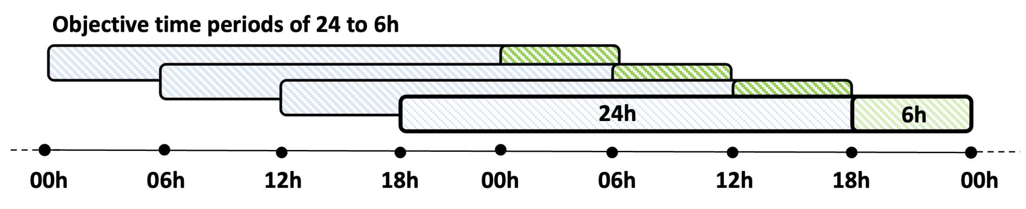
The recruited patients wore different sensors, including the Dexcom G6, the MiniMed 640G, and the FreeStyle Libre. The first two sensor models stored their measurements every 5 min, while the third model stored its measurements every 15 min. First, CGM measurements were preprocessed. Then, 24 h periods starting at 0 h, 6 h, 12 h, and 18 h and their corresponding subsequent period of 6 h were obtained (Figure 1). The measurements in each period are divided into the five previously mentioned glucose ranges.
The patients’ glucose profiles have unrecorded measurements. Data were linearly interpolated when the gaps of missing data were not greater than two consecutive hours. The missing data that was interpolated is actual missing data. Surely if smaller periods were interpolated or not interpolated at all the quality of the data would improve. In this procedure, the days that had more than 2 h of missing data in the same period of 6 h were eliminated. Finally, a day was considered valid if each of its four 6 h periods had at least 75% of the data. Table 2 shows the total number of days analyzed, sensors, and valid periods of 24 h and consecutive 6 h periods for each patient.

2.2. CoDa

A composition is a vector X = ( x 1 , x 2 , , x D ) , with D number of parts whose components are all strictly positive and of constant sum (which can be the unit, 100% (as is our case study), sum of the hours of the day (24 h) or some other constant sum defined by the researcher), according to the “scale invariance” property the chosen value for k it is irrelevant for the analysis and is only useful for the interpretation of the results:
x i > 0 , i = 1 , 2 , , D . i = 1 D x i = k k = c t e .
Historically, CoDa have been identified with closed data, with the simplex being the natural sample space for this data type, while the real Euclidean space is associated with unrestricted data. The basic principles of CoDa analysis that are of special interest in this study are as follows:
(1) scale invariance, which states that CoDa only contains relative information, implying that any change in the scale of the original data do not affect the structure of the composition;
(2) subcompositional coherence, which implies that the results obtained for a subset of parts of a composition, that is, a subcomposition, must be coherent with the results obtained with the complete composition; and
(3) permutation invariance, which indicates that the results do not depend on the order in which the parts appear in the composition [14].
In this work, the compositional vector X is defined as a composition where each D-part corresponds to the percentage of time in each of the glucose ranges:
  • Hypoglycemia level 2 ( X < 54 ) ,
  • Hypoglycemia level 1 ( X 54 70 ),
  • Target BG ( X 70 180 ),
  • Hyperglycemia level 1 ( X 180 250 ), and
  • Hyperglycemia level 2 ( X > 250 )
and is treated as the 5-part composition:
X = ( X < 54 , X 54 70 , X 70 180 , X 180 250 , X > 250 ) .
whose constant sum is 100%. Some of the parts of the composition would be zero if no measurements were found in some of the glucose ranges. For example, a composition (0, 0, 100, 0, 0) would mean 100% TIR, another example could be (0, 10, 80, 10, 0) where it would have 10% in hypo and hyper level 1 and 80% in TIR. As CoDa analysis is based on log-ratios of parts, treating zeros appropriately and analyzing incidence patterns is necessary [20]. In the analyzed measurements, three types of patterns of zeros were identified: non-consecutive zeros, two consecutive zeros, and three consecutive zeros.
The detection limits ( d l ) matrix used in zero imputation was obtained considering 5- and 15-min fractions, as in Biagi and colleagues [12], depending on the position of the zero in the compositions. For the sensors that save the measurements every 5 min, one day has 1440/5 = 288 measurement recordings, then the d l is calculated as d l = 5/1440 = 1/288 = 0.0035; following the same procedure for the sensors that store the samples every 15 min, 1440/15 = 96 measurements, then the d l = 15/1440 = 1/96 = 0.0104. Measured values below the thresholds defined in the d l matrix cannot be distinguished from a blank signal with a specified confidence level. We considered that the further the zero is from the non-zero value, the smaller this value must be in the d l matrix, as presented in Table A5 of Appendix A. In none of the periods, the glucose range was found to be always zero for any patient. Therefore, we consider these zeros to be rounded zeros of continuous data, not essential ones.
The replacement of zeros in the vector of times at each of the glucose ranges is performed following Biagi and colleagues [12] using the robust expectation-maximization (lrEM) [20,21]. This model-based function imputes left-censored data (e.g., values below the d l , rounded zeros) by representing CoDa coordinates incorporating the relative covariance structure information. When the matrix of zero patterns has a whole column of zeros, the multiplicative replacement method (multRepl) [20,22] was considered. This method preserves the covariance structure and is consistent with the properties of CoDa; it consists of multiplicatively imputing the null values with a small preset value. The modification in the values that are not zero is multiplicative; it is consistent with the basic operations in the simplex and the structure of the compositions [23,24]. Figure 2 describes the methodology for this work, first for proper preprocessing of BG measurements, then for the validation of the model, and finally, the update of the probabilistic prediction model if it has already been previously validated.

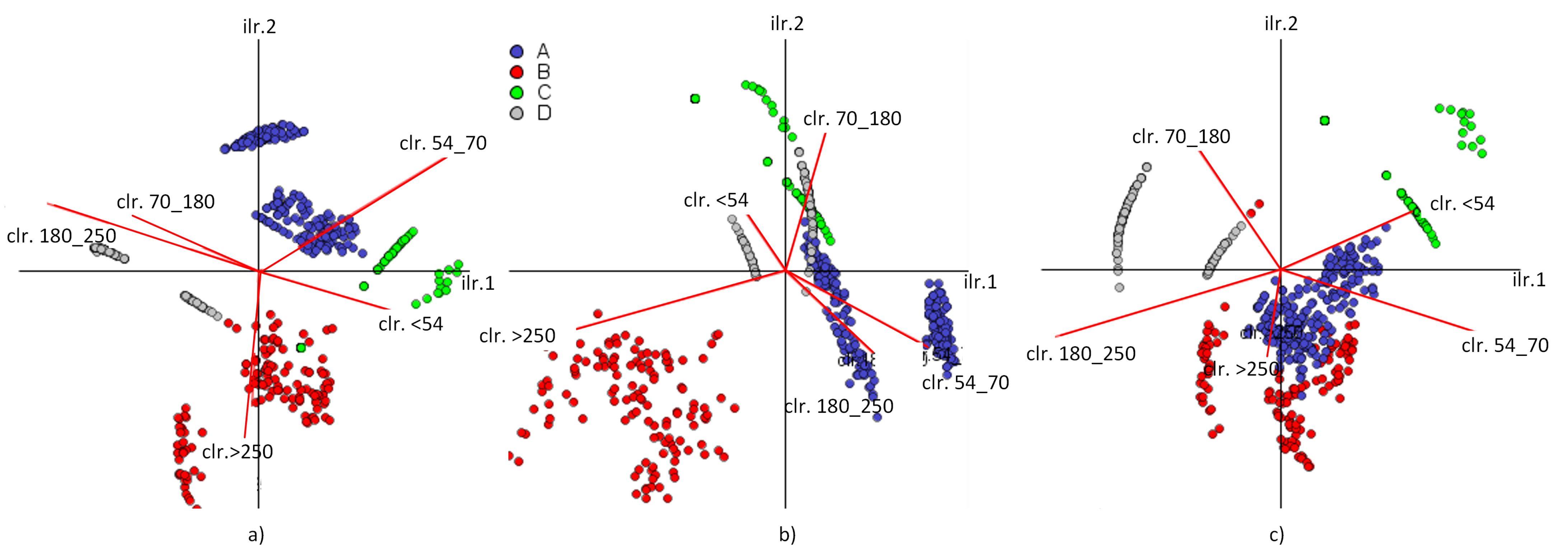
2.2.1. Log-Ratio Coordinates

CoDa can be translated into real space via clr-scores and olr-coordinates, in which, traditional statistical methods can be applied [14], and are calculated using Equations (3) and (4) [25], where g is the geometric mean (Equation (5)), r and s are the number of parts in the i-th row of S (sign matrix of the sequential binary partition (SBP)) coded by +1 (positive) and −1 (negative), which will be in the numerator and denominator of the corresponding log-ratio, respectively. Egozcue and Pawlowsky-Glahn [26] defined the SBP as a hierarchical grouping of parts of the original compositional vector, starting with the complete composition as a group and ending with each part in a single group. If D is the number of parts in the original composition, then the number of steps in the partition is D 1 . In this study, we considered the SBP presented in Table 3, which was established according to Biagi and colleagues [12].
c l r ( x ) = c l r 1 , c l r 2 , , c l r D = ln x 1 g ( x ) , ln x 2 g ( x ) , , ln x D g ( x ) .
o l r ( x ) = r s r + s ln g ( x + ) 1 r g ( x ) 1 s .

2.2.2. Compositional Measurements

The geometric mean is a representative measure of the center of the CoDa set and identifies the components that better discriminate in the composition. Let X = ( x 1 , x 2 , , x n ) be a compositional data set of S D . The compositional geometric mean ( g k ) of the set X is defined as:
g ( X ) = g 1 , g 2 , , g D = g 1 g k , g 2 g k , , g D g k , g k = i = 1 n x i k 1 n .
where g k represents the geometric mean represents the geometric mean of the k-th component of the data. The variation matrix shows the pairwise log-ratio variance for all parts of the composition. It allows the analysis of the data dispersion. This matrix is defined as T = [ T i j ] , and in its extended form, is equal to:
T = T i j = v a r ln x 1 x 1 v a r ln x 1 x D v a r ln x D x 1 v a r ln x D x D .
where T i j = v a r [ ln ( x i / x j ) ] represents the expected variance of the log-ratio of parts i and j. This matrix is based on the contribution of variance for each pairwise log-ratio. However, the variation array is usually preferred in practice. This array is based on the variation matrix where the upper diagonal of the array contains the log-ratio variances and the lower diagonal contains the log-ratio means. That is, the way we show the results in Table A2 of the Appendix A, the i j -th component of the upper diagonal is var [ ln ( X i / X j ) ] and the i j -th component of the lower diagonal is E [ ln ( X i / X j ) ] , where i, j = 1 , 2 , , D [14].
In real space, the most widely used measure of dispersion is the trace of the covariance matrix associated with the ensemble. However, the interpretability of the direct covariance matrix of a CoDa set is lacking. As this measure is not compatible with CoDa, Pawlowsky-Glahn and Egozcue [16] defined a measure of variability t o t v a r ( X ) equal to the trace of the covariance matrix of the clr-transformed data set:
t o t v a r ( X ) = k = 1 D v a r [ c l r k ( x ) ] .
An example of specific results of these measures for patient 1 (P1) can be observed in Table A1 and Table A2 of the Appendix A.

2.3. Probabilistic Model of Transition

The probabilistic transition model proposed by Biagi et al. [13] was implemented for 3, 4, and 5 clusters, where the categories from the previous 24 h period to the next 6 h period are counted. The procedure is as follows: suppose the categories are defined as A, B, C, D, and E. First find all the A categories, examine the period after these days and complete a matrix with the counts of each column, as described in Table 4. Then, with the closure operator defined in Equation (8), the transition probabilities are calculated at different times of the day. Table A3 of the Appendix A shows a particular example of the model for P1.
X 1 , X 2 , , X D = X 1 i = 1 D X i , X 2 i = 1 D X i , , X D i = 1 D X i .
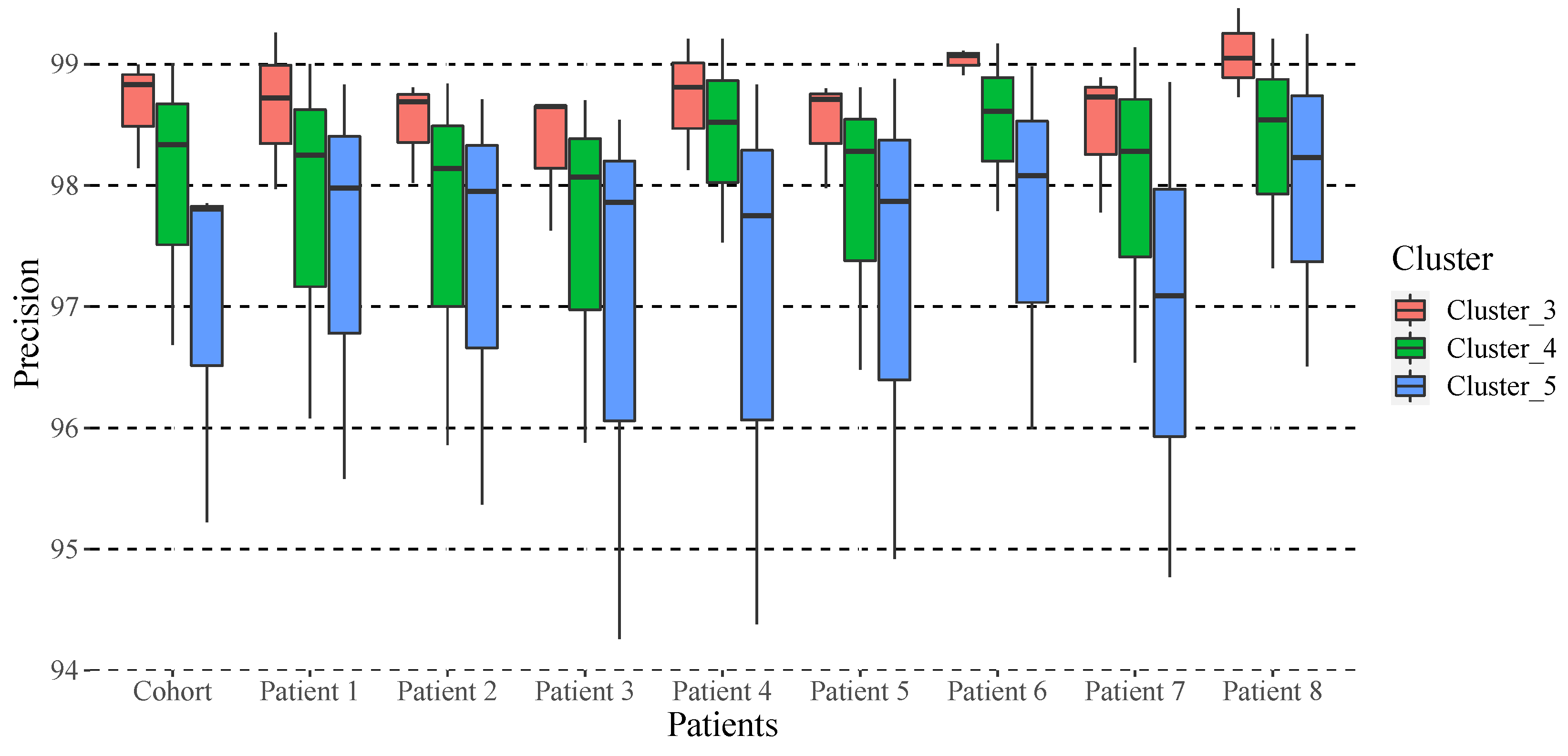
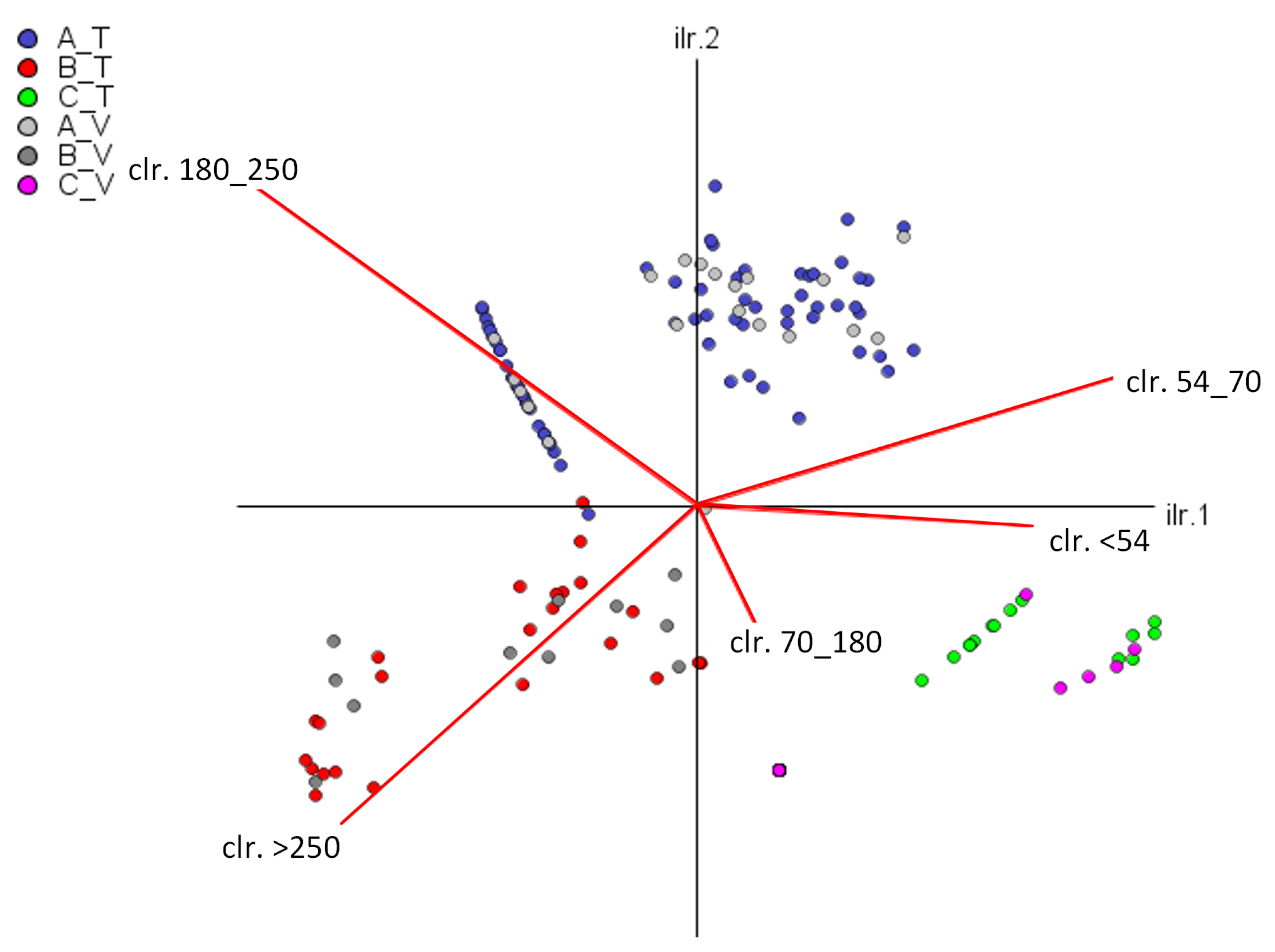
To validate this probabilistic transition model, clusters 3, 4, and 5 mentioned previously are analyzed. We consider 5-fold cross-validation, randomly selecting 75% of the data for training and the remaining 25% for validation. We employ linear discriminant analysis to assign groups to the validation data, following the methodology of Biagi et al. [13]. Both the training and validation data of the model are CoDa vectors, whose constant sum is 100%. Therefore, a metric is needed to compare the training and validation results to obtain the accuracy of the model.

2.4. Accuracy Metric

We propose the calculation of an accuracy metric based on CoDa. The first step is to create the Training (T) and Validation (V) matrices (Equation (9)), which contain the transition probabilities of the categories from one 24 h period to the next 6 h, where D is the dimension of the vector. For this, the categories are counted, and the zero type counts are substituted.
In Martín-Fernández et al. [27], count-type vectors are defined as categorical data in which the counts represent the number of elements located in each of several categories. This type of zeros is related to a sampling problem because the components may not be observed given the limited size of the sample. The count-zero multiplicative replacement is implemented in the R package “zCompositions” [20], following what was established in Martín-Fernández et al. [27], where the multiplicative replacement by rounded zero defined in Martín-Fernández and colleagues [24] was adapted for the case of counting zeros. Although this method satisfies the condition that the imputed zero value does not depend on the D parts of the composition, it is recommended only when the number of zeros in the data matrix is insignificant.
T = T 11 T 1 D T D 1 T D D V = V 11 V 1 D V D 1 V D D .
The accuracy is a difference measure between the training data (expected), and the validation data (observed) for each k model created. The higher the accuracy, the more similar the probability vectors between the transitions from one period to another; therefore, it would also suggest the most appropriate number of groups for each patient. From the analysis of the distances and the norms of the T and V vectors that are detailed below, the accuracy metric is defined as Equation (10).
A c c u r a c y = 100 | | V T | | a | | V | | a + | | T | | a 100 .
To implement this Equation (10), mathematical operators defined for CoDa were considered. The T or V matrix vectors where no transitions were found from one period to another were treated as null or empty ( ) . Then, the difference perturbation operator introduced by Martín-Fernández and their colleagues [9] is applied as:
X Y = X 1 Y 1 , X 2 Y 2 , , X D Y D .
Applying Equation (11) to the previously defined matrices T and V leads to Equation (12). The perturbation difference operation is analogous to subtraction in Euclidean space. Therefore, the process is performed row-wise.
V T = V 11 V 1 D V D 1 V D D T 11 T 1 D T D 1 T D D = V 11 T 11 V 1 D T 1 D V D 1 T D 1 V D D T D D .
The difference perturbation operation also includes the closure operator ( ) , as defined in Equation (8). This is a technique to simplify the use of closed-form compositions, that is, positive vectors whose parts add up to a constant positive k (in our case, k = 100 % , percentage type data). In this context, the triangular inequality theorem of Euclidean geometry is applied, which has been generalized to normed vector spaces, obtaining:
| | V T | | a | | V | | a + | | T | | a .
where the Aitchison norm | | · | | a of a composition can be calculated as the Euclidean norm | | · | | of the clr-scores [25].
| | V T | | a = | | c l r ( V T ) | | = i = 1 D c l r i ( V T ) 2 .
| | V | | a = | | c l r ( V ) | | = i = 1 D c l r i ( V ) 2 .
| | T | | a = | | c l r ( T ) | | = i = 1 D c l r i ( T ) 2 .
Rearranging Equation (13), we obtain:
0 | | V T | | a | | V | | a + | | T | | a 1 .
The Aitchison distance [28] between two compositions is known as d a ( X , Y ) (Equation (18)), which is the norm of the difference perturbation operation of these compositions; therefore, in the numerator of Equation (17), the Aitchison distance of the composition created between the components of the training vector and those of the validation vector is calculated.
d a ( X , Y ) = | | X Y | | a .

2.5. Precision Metric of the Transition Model

In this work, we also propose the adaptation of known statistical errors in terms of CoDa. This is achieved through the transformation of basic Euclidean operations of the mathematical equations to their corresponding operation in the simplex, as follows:
M A E = e a = 1 t o t a l k = 1 t o t a l | | V D T D | | a .
M R E = e r = e a | | T D | | a .
R M S E = e c = k = 1 t o t a l | | V D T D | | a 2 t o t a l .
where:
  • e a : mean absolute error (MAE)
  • e r : mean relative error ( M R E )
  • e c : root mean square error ( R M S E )
  • D is the number of parts of the composition
  • V D : is the observed composition (that is, the data validation)
  • T D : is the expected composition (the training data)
  • t o t a l : is the number of corresponding vectors for each 5-fold
  • k = 3, 4 or 5: corresponds to the number of clusters being analyzed
The precision of the model is calculated according to:
P r e c i s i o n = 100 e a 100 e r 100 e c .

3. Results

The median accuracy after 5-fold validation for 3, 4, and 5 clusters are presented in Table 5 for the cohort. Accuracy greater than 50 % is considered exceptionally good, indicating that at least half of the parts of the composition coincided satisfactorily (i.e., the data of V with the data of T). Clarifying that as the clusters increase, the T vector and the V vector also increase, is necessary. Therefore, more probabilities of dissimilarity exist among the parts of the vectors, which causes the result of the accuracy measurement to decrease. As evident from Table 5, the accuracy results for 3 clusters are larger than those for 5 clusters. The probabilistic model has been successfully validated because the validation data confirms what was predicted by the training data. The Appendix illustrates an example of the application of this proposed metric for P1.
The box plot of Figure 3 shows the summary of the precision based on the errors of the validation of the probabilistic transition model for clusters 3, 4, and 5 of each one of the patients and the cohort in general. The top of the box (third quartile) illustrates that 75 % of the values are less than or equal to this ( 98 % ), the bottom of the box (first quartile) shows that 25 % of the values are less than or equal to this value ( 94 % ). The median (second quartile) divides the distribution into two equal parts. For cluster 3, only P1 has a symmetric precision distribution (mean, median, and mode coincide), although for the remaining patients, as well as the cohort, the median has a negative asymmetry or is skewed to the left (the longest part below the median). Thus, the data is concentrated in the upper part of the distribution and the mean is less than the median. This same behavior is evident for all the clusters, indicating that in all cases, the lower part of the boxes is larger (the data is more dispersed). Notably, the respective clusters of each patient exhibit similar behavior. However, cluster 5 of patients 3 and 4 stands out—their minimum precision was close to 94 % and this was due to the variability of the patients ( 43 % and 39.6 % , respectively). In all cases, the dimensions of the boxes determined by the distance of the interquartile range grew as the clusters increased, which evidences the dispersion of the data around the median, and in turn, reflects how it coincides with the results of the accuracy (the greater the number of clusters, the lower the number of samples per group).
These results are relevant for the research, application, and validation of CoDa methodologies in any branch of science. The metrics obtained allow the comparison of dissimilar compositions, the disregard of parts of the composition that are not significant, the validation of models, and the identification of patterns. However, it is important to highlight that the researcher is the one who proposes, based on their experience in the field, the parts of the composition and the constant to be added according to the characteristics of CoDa, so they must also interpret the results obtained. Furthermore, as previously mentioned, the more parts the composition vector has, the greater the possibility that the accuracy metric will be lower. Therefore, the percentage obtained by this metric will be associated with the interpretation given by the researcher.

4. Discussion

Data-driven decision support systems have always helped physicians and patients [4,5]. This work is the continuation of previous studies to characterize glucose profiles of times in different ranges applying CoDa. Biagi and colleagues [12] created a methodology for the categorization of glucose profiles of six T1D patients who were monitored for eight weeks. Then, the k-means algorithm was applied to the clr-scores, obtaining different groups. Subsequently, Biagi et al. [13] obtained a discriminant model to determine the category of 24 h periods, achieving an average of more than 94 % correct classification. Furthermore, the authors proposed a probabilistic transition model to predict the future 6 h period.
These two investigations set the path to the CoDa analysis tool applied to the glucose profiles of patients with T1D. However, a validation of the probabilistic transition model obtained in Biagi et al. [13] was not presented, which is considered a limitation of the study by the authors. This model would serve as a decision support tool to manage T1D for patients and physicians. In this study, the limitations of [12] are minimized by comprehensively analyzing the compositional statistics of these data, which provides valuable information on the behavior of glucose, traceability, and improvement of the patient’s glucose profiles. Thus, the characteristics of the classificatory groups are identified not only qualitatively but also quantitatively, as stated in [12]. In addition, other methodologies were tested to determine the detection limits matrix of the data set; however, placing a lower d l on zero parts farther from the non-zero parts had less effect on variability.
Finally, the probabilistic prediction model is validated to ensure its reliability. Notably, during the validation of the model, the greater the number of groups, the fewer the observations per group, which suggests lower percentages for each part because of the distribution of the category counts. Hence, the relevance of accuracy. A new accuracy metric based on the difference in compositional vectors was proposed in this work, which allowed the validation of the proposed prediction model. The validation of the model provides an idea of what the correct amount of cluster should be for each patient to achieve the highest accuracy in the prediction.
In some cases, the measure of the accuracy of some transition probabilities was not high. This happens fundamentally because of the few days, which leads to sufficient transitions not being always counted in some cases, creating a model where the probability percentages are dispersed. Similarly, we consider that the update of the model and incorporation of more recent data improves the reliability of prediction, including predicting for a shorter period. This would help clinicians to assess patient outcomes and to customize their insulin dosing profile.
This methodology is designed for an individualized probabilistic transition model and not for the cohort. As mentioned in [13], in this study, we did not intend to present the prediction of BG values or trends but a probability of the behavior of glucose in the following 6 h as a decision support tool for the management of T1D. Furthermore, considering that glucose sensors lack of accuracy, patients’s insulin sensitivity and the dynamic of insulin response in the body are also estimations, there is not a method that could guarantee the verification of the effects of insulin in the glucose drop. In that way, the prediction of the behavior of the patient through the category obtained from composition of times in different glucose ranges in future periods could decrease the effects of intrinsic inaccuracies of devices used for diabetes management that can jeopardize patient care. The intent was that, as the model suggests the patient, it will be updated and adjusted considering the habits and characteristics of individual patients over time.

5. Conclusions

In this work, a novel methodology was presented to validate the probabilistic transition model presented in [13]. New measures of accuracy and precision based on CoDa were proposed. Glucose measurements from eight T1D patients were processed. Obtaining satisfactory average results with accuracy and precision greater than 50 % and 95 % for the entire cohort, respectively, suggests the reliability of the model. This methodology can be extended to CoDa analysis for other studies that need to be validated or for comparisons between compositions where the components represent parts of a whole. The novelty of this work stems from the absence of this type of measure in the extant literature.

Author Contributions

A.C. and L.B. wrote the manuscript, contributed to discussion, and reviewed/edited the manuscript; conceptualization, A.C., J.V. and J.A.M.-F.; methodology, A.C.; software, A.C., L.B., E.E., A.B. and I.C. (Iván Contreras); validation, A.C., E.E., A.B., I.C. (Iván Contreras) and J.B.; investigation, A.C.; writing—review and editing, A.C., E.E., L.B., A.B., I.C. (Iván Contreras), J.A.M.-F., M.G., I.C. (Ignacio Conget) and J.V.; funding acquisition, A.C., E.E. and J.V. All authors have read and agreed to the published version of the manuscript.

Funding

This research was partially supported by grants PID2019-107722RB-C22 and PID2019-107722RB-C12 funded by MCIN/AEI/10.13039/501100011033, in part by the Autonomous Government of Catalonia under Grant 2017 SGR 1551, in part by the Spanish Ministry of Universities, and by the European Union through Next GenerationEU (Margarita Salas), and by the program for researchers in training at the University of Girona (IFUdG2019).

Institutional Review Board Statement

The study was conducted in accordance with the Declaration of Helsinki.

Informed Consent Statement

Informed consent was obtained from all subjects involved in the study.

Data Availability Statement

Not applicable.

Acknowledgments

The authors thank all the participants who dedicated their time and effort to complete this study.

Conflicts of Interest

The authors declare no conflict of interest.

Abbreviations

The following abbreviations are used in this manuscript:
T1DType 1 diabetes
TIRTime in range
BGBlood glucose
MDIMultiple daily injections
CSIIContinuous subcutaneous insulin infusion
CGMContinuous glucose monitoring
CoDaCompositional Data
clrCentered log-ratio
ilrIsometric log-ratio
SBPSequential binary partition
BGVBlood glucose variation
CHOCarbohydrate
SDStandard deviation
SEMStandard error of the mean
MAEMean absolute error
MREMean relative error
RMSERoot mean square error
P1Patient 1

Appendix A. Specific Results for P1

Appendix A.1. Compositional Statistics of the Data

Once the 24 h and 6 h consecutive data have been categorized with the k-means method, the different groups are obtained (in this example, 4 groups were set). The compositional geometric mean is calculated for each of these groups (Equation (5)). This vector provides a quantitative interpretation of each of the groups (Table A1). The 24 h and 6 h periods were qualitatively characterized in terms of the relative time spent in the different glucose ranges, according to the log-ratio approach. Although groups of different patients may present comparable characteristics in terms of the relative interpretation of the time spent in different glucose ranges, the results must be interpreted individually and in a relative sense and not in an absolute manner. Both the 24 h and 6 h periods were classified taking into account the standardized metrics [8] where the following glucose targets are pursued: <54 mg/dL (<1%), 54–70 mg/dL (<4%), 70–180 mg/dL (>70%), 180–250 mg/dL (<20%) and >250 mg/dL (<5%). If we analyze the example shown in (Table A1) we can see that group 1 has an average of 2.61% in hypo level 1, 87.38% in TIR and 10% in hyper level 1. In view of these data, we assign classification A, which we will qualitatively define as periods with a moderate percentage of hypo and hyper level 1. Following this logic, for this example, the groups are classified as follows:
The 24 h periods were classified as:
• A—periods with percentages in hyperglycemia and moderate hypoglycemia of level 1.
• B—periods with high percentages of level 1 and level 2 hyperglycemia.
• C—periods with high percentages of time in range with slight occurrences of level 1 hypoglycemia.
• D—periods with percentages of level 1 hyperglycemia.
The 6 h periods were classified as:
• A—periods with percentages in level 1 hyperglycemia and hypoglycemia.
• B—periods with very high percentages of level 1 and level 2 hyperglycemia.
• C—periods with high percentages of time in range.
• D—periods with percentages of level 1 hyperglycemia.
Table A1. Compositional center of each of the parts by a group of P1.
Compositional center of each group of 24 h periods for group 4
G_A(179)G_B(96)G_C(23)G_D(37)
<54   [mg/dL]0.000.000.000.00
54–70   [mg/dL]2.610.990.220.00
70–180   [mg/dL]87.3876.1899.7786.47
180–250   [mg/dL]1018.790.0013.52
>250   [mg/dL]0.004.020.000.00
Compositional center of each group of the next period of 6 h for group 4
G_A(67)G_B(33)G_C(119)G_D(116)
<54   [mg/dL]0.000.000.000.00
54–70   [mg/dL]5.650.000.000.00
70–180   [mg/dL]80.0051.2399.9583.28
180–250   [mg/dL]14.3432.540.0016.72
>250   [mg/dL]0.0016.210.000.00
Median and percentile (25th,75th) of each of the parts by group
G_A(246)G_B(129)G_C(142)G_D(153)
<54   [mg/dL]0.00 (0.00–0.69)0.00(0.00–0.69)0.00(0.00–0.00)0.00(0.00–0.00)
54–70   [mg/dL]3.47(1.39–5.56)1.39(0.00–3.47)0.00(0.00–5.21)0.00(0.00–0.00)
70–180   [mg/dL]83.33(74.31–89.58)68.06(55.21–77.43)100(94.44–100)83.33(72.22–91.67)
180–250   [mg/dL]12.15(6.60–19.79)20.83(15.28–26.74)0.00(0.00–0.00)16.67(8.33–27.78)
>250   [mg/dL]0.00(0.00–0.00)5.90(2.43–13.89)0.00(0.00–0.00)0.00(0.00–0.00)
Group (Number of observations per group).
Table A2. Variation array of P1.
Variances ln ( X i X j )
X i X j <5454–7070–180180–250>250clr variances
<54 14.573618.726934.820516.67937.1033
54–703.7926 26.844041.936029.966012.8072
70–18011.00207.2094 15.608519.60586.3003
180–2507.30203.5094−3.7001 27.658514.1479
>2500.3664−3.4262−10.6357−6.9356 8.9251
Mean ln ( X i X j ) TV: 49.28
Table A2 shows the variation array of the data for P1 (according to Equation (7)). The greatest compositional variability is associated with the parts (180–250) with (<54–70) (41.9), (180–250) with (<54) (34.8), and (>250) with (54–70) (29.9) (bold font). According to [29], the components with the greatest variability turn out to be adequate to obtain a subcomposition of three parts and illustrate the data dispersion. The total variance (TV) for this data set was 49.28, and (54–70) with 12.8, (180–250) with 14.14, and (>250) with 8.9 being the parts with the largest contribution (see column clr variances in Table A2).

Appendix A.2. Compositional Biplot for P1 Categorized for 4 Clusters

Akin to classical statistical analysis, CoDa analysis requires data visualization tools; one tool is the compositional biplot [30]. The biplot is a dimensional reduction technique used to represent data with three or more variables. This technique aims to approximate the elements of a matrix from vectors called markers associated with the rows and columns [31].
In this work, the rows correspond to the days and are displayed as points in the compositional clr-biplot. The columns correspond to the times in each of the glucose ranges, represented as rays. The quality of the representation depends on the percentage of variance that is retained with the two axes that are represented. It is constructed by obtaining a singular value decomposition of the covariance matrix using the clr transformation. The interpretation is based on the links between the rays: each ray represents a clr variable, and its length is associated with the variance explained in the projection. The directions of the rays indicate those observations with a greater domain of the compositional part [29]. Figure A1 illustrates the distribution of days when they have been categorized into four clusters from different perspectives and the retained variance.
Figure A1. Compositional biplot in space for P1: (a) XY plane; (b) YZ plane, and (c) XZ plane. The three axes of the biplot retain 51 % , 77 % , and 90 % of the TV, respectively.
Mathematics 11 01241 g0a1

Appendix A.3. Probabilistic of Transition Model

Table A3 shows the probabilities of transition at different times of the day (0 h, 6 h, 12 h, and 18 h) for P1. Let us consider the patient at 18 h when they have been categorized with four clusters. First, we analyze the glucose composition of the previous 24 h period using Table A1 (Compositional center of each group of 24 h periods) and verify that this period is categorized as type D (86.47% in normoglycemia and 13.52% in hyperglycemia, no hypos observed). Then the probability that the category of the next 6 h period (from 18 h to 0 h) is of type D 75% can be known. Table A1 (Compositional center of each group of 6 h periods) demonstrates how group D was characterized by having 83.28% time in normoglycemia and 16.72% in hyperglycemia. In other words, P1 is expected to continue in normoglycemia with a tendency to hyperglycemic excursions for the next 6 h.
Table A3. Probabilistic transition model for clusters 3, 4, and 5 for P1.
At 0 hAt 6 hAt 12 hAt 18 h
ABCDEABCDEABCDEABCDE
A23.046.130.7 31.131.137.7 40.423.436.1 50.921.527.4
B28.048.024.0 20.631.048.2 30.726.942.3 46.130.723.0
C25.012.562.5 22.233.344.4 50.040.010.0 14.214.271.4
A10.617.044.627.6 13.92.346.537.2 29.54.529.536.3 37.76.628.826.6
B4.321.752.121.7 16.020.012.052.0 17.313.026.043.4 36.012.032.020.0
C0.00.042.857.1 0.00.060.040.0 0.020.060.020.0 16.60.050.033.3
D12.50.025.062.5 10.010.040.040.0 36.39.036.318.1 12.50.012.575.0
A5.020.015.025.035.00.00.07.135.757.10.00.042.121.036.816.60.016.633.333.3
B4.321.70.052.121.70.020.812.512.554.113.613.64.522.745.48.012.028.032.020.0
C0.014.83.759.222.23.33.316.650.026.60.07.619.238.434.614.811.125.925.922.2
D0.00.00.042.857.10.00.00.060.040.00.020.00.060.020.016.60.00.050.033.3
E0.00.012.525.062.510.010.00.040.040.00.09.036.336.318.10.00.012.512.575.0

Appendix A.4. Analysis of the Result of the Accuracy Metric for P1

The median accuracy and interquartile range after 5-fold validation for 3, 4, and 5 clusters for P1 is shown in Table A4. It was observed that considering 3 clusters in the evaluation resulted in higher accuracy compared to the evaluation with 5 clusters. Furthermore, it was found that the median accuracy for this particular patient significantly exceeded the cohort median, approaching 90% in the 75th percentile.
Table A4. Accuracy results after 5-fold cross-validation for P1.
Cluster At 0 hAt 6 hAt 12 hAt 18 h
3A67.2 (66.3–77.2)83.9 (55.6–84.6)80.1 (78.2–83.8)80.4 (72.2–83.3)
B54.6 (2.1–68.7)75.1 (66.9–76.7)61.7 (52.6–73.2)69.1 (39.3–71.0)
C55.6 (44.8–69.9)86.1 (62.8–86.7)40.3 (19.4–48.5)58.6 (52.6–65.6)
4A59.8 (45.7–72.0)83.7 (24.3–88.6)74.3 (39.7–78.9)69.8 (67.5–75.3)
B56.7 (44.9–63.1)64.9 (58.4–67.8)46.1 (28.2–47.9)45.3 (33.7–63.0)
C47.7 (42.8–49.4)64.6 (60.2–66.4)35.8 (18.6–46.6)43.9 (31.8–56.7)
D45.7 (32.2–66.1)38.8 (24.1–54.8)20.6 (13.8–37.6)54.6 (39.3–64.7)
5A44.0 (29.2–55.2)44.8 (36.3–61.9)25.4 (18.2–60.5)43.8 (11.1–57.4)
B60.9 (47.1–65.8)51.3 (42.4–62.1)33.9 (6.6–44.5)48.3 (31.9–60.5)
C50.7 (39.8–58.6)46.2 (30.8–71.3)58.8 (39.3–62.5)48.8 (33.5–58.2)
D36.2 (30.7–36.7)60.6 (34.6–64.7)30.8 (21.0–34.6)35.5 (22.7–53.9)
E20.5 (16.4–40.8)28.3 (8.6–46.9)13.0 (10.2–23.5)48.8 (37.9–54.1)
The result is the median (interquartile range (25th–75th)) of the accuracy for the validation of the probabilistic transition model for P1.
Below is an example of the accuracy metric for P1, for k-fold = 2, when the transitions at 0 h to the next period of 0–6 h are counted. After categorizing with k-means the clr-scores corresponding to the times in the range. The categories from the 24 h to the next 6 h period of the T and V data are counted, which in this case, were T = [19 16 7] and for V = [6 2 6]. Then, these vectors are verified as not having zeros; in case they do, they are replaced as explained in Section 2.4. Subsequently, Equation (8) is applied, whose constant sum is 100 % and can be treated as a CoDa, and T = [45.23 14.28 40.47] and V = [42.85 14.28 42.85] are obtained.
Calculating the numerator for Equation (10): Applying the difference operator (Equation (11)) and then the closure operator (Equation (8)):
V T = V 1 T 1 , V 2 T 2 , V 3 T 3 = 42.85 45.23 , 14.28 14.28 , 42.85 40.47 = 0.9474 , 1 , 1.0588 = 0.3151 , 0.3326 , 0.3522 .
Then, the clr-scores are calculated according to Equation (3) and the denominator of the clr-scores (the geometric mean) is calculated according to Equation (5).
c l r ( V T ) = c l r ( 0.3151 , 0.3326 , 0.3522 ) = ln 0.3151 0.3330 , ln 0.3326 0.3330 , ln 0.3522 0.3330 = 0.0551 , 0.0010 , 0.0561 .
Applying Equation (14), the norm of the clr-scores is calculated as:
| | V T | | a = ( 0.0551 ) 2 + ( 0.0010 ) 2 + ( 0.0561 ) 2 = 0.0786 .
Calculating the denominator: According to Equation (3), the clr-scores are first calculated, where the geometric mean g ( V ) = 27.70 and g ( T ) = 29.67 according to Equation (5). Subsequently, the Aitchison norm of the vectors V and T is calculated (Equations (15) and (16)).
c l r ( V ) = ln 42.85 29.70 , ln 14.28 29.70 , ln 42.85 29.70 = 0.3663 , 0.7326 , 0.3663 .
c l r ( T ) = ln 45.23 29.67 , ln 14.28 29.67 , ln 40.47 29.67 = 0.4214 , 0.7315 , 0.3102 .
| | V | | a = | | c l r ( V ) | | = ( 0.3663 ) 2 + ( 0.7326 ) 2 + ( 0.3663 ) 2 = 0.8972 .
| | T | | a = | | c l r ( T ) | | = ( 0.4214 ) 2 + ( 0.7314 ) 2 + ( 0.3102 ) 2 = 0.8994 .
Finally substituting in Equation (10):
A c c u r a c y = 100 | | V T | | a | | V | | a + | | T | | a 100 = 100 0.0786 0.8972 + 0.8994 100 = 95.62 % .
Figure A2 shows the previously discussed example of accuracy in compositional biplot, where: A _ T , B _ T , and C _ T correspond to the training data and A _ V , B _ V , and C _ V to the validation data when the data have only been categorized for three clusters. How related the T and V data are in each cluster is evident. In addition, the length of all the pairwise links between the rays suggests no redundant information. That is, amalgamating parts is not recommended. The variance retained by the two first axes in the biplot is 79%, implying that it has high quality, thus suggesting caution in the interpretations.
Figure A2. Example of visualization of training and validation data for P1.
Mathematics 11 01241 g0a2

Appendix A.5. Detection Limits

Table A5 shows the detection limits for different patterns of zeros.
Table A5. Detection limits for different patterns of zeros.
For measurements recorded every 5 min. 1440 min/5 min = 288 measurements dl = 1/288 = 0.0035
Consecutive zerosPosition 1Position 2Position 3Position 4
1dl = 0.0035
2dl/3 = 0.00122dl/3 = 0.0023
3dl/9 = 0.000382dl/9 = 0.000772dl/3 = 0.0023
4dl/27 = 0.000122dl/27 = 0.000262dl/9 = 0.000772dl/3 = 0.0023
For measurements recorded every 15 min. 1440 min/15 min= 96 measurements dl = 1/96 = 0.010
1dl = 0.010
2dl/3 = 0.00332dl/3 = 0.0067
3dl/9 = 0.00112dl/9 = 0.00222dl/3 = 0.0067
4dl/27 = 0.000372dl/27 = 0.000742dl/9 = 0.00222dl/3 = 0.0067

References

  1. da Silva, J.A.; de Souza, E.C.F. Diagnosis of diabetes mellitus and living with a chronic condition: Participatory study. BMC Public Health 2018, 18, 1–8. [Google Scholar] [CrossRef] [PubMed] [Green Version]
  2. Jeitler, K.; Horvath, K.; Berghold, A. Continuous subcutaneous insulin infusion versus multiple daily insulin injections in patients with diabetes mellitus: Systematic review and meta-analysis. Diabetologia 2008, 51, 941–951. [Google Scholar] [CrossRef] [PubMed] [Green Version]
  3. Livvi, S.; Wei, L.; Kim, B.K.H.; Wee, T.T. Development of a clinical decision support system for diabetes care: A pilot study. PLoS ONE 2017, 12, e0173021. [Google Scholar]
  4. Tyler, N.S.; Jacobs, P.G. Artificial intelligence in decision support systems for type 1 diabetes. Sensors 2020, 20, 3214. [Google Scholar] [CrossRef]
  5. Ivan, C.; Josep, V. Artificial intelligence for diabetes management and decision support: Literature review. J. Med. Internet Res. 2018, 20, e10775. [Google Scholar]
  6. Revita, N.; Tadej, B. Insulin dose optimization using an automated artificial intelligence-based decision support system in youths with type 1 diabetes. Nat. Med. 2020, 26, 9. [Google Scholar]
  7. Ellahham, S. Artificial intelligence: The future for diabetes care. Am. J. Med. 2020, 133, 8. [Google Scholar] [CrossRef]
  8. American Diabetes Association. Care in Diabetes-2022. Diabetes Care 2022, 17, 254–255. [Google Scholar]
  9. Fernández, M.; Antoni, J.; Estadella, D. On the interpretation of differences between groups for compositional data. Sort Stat. Oper. Res. Trans. 2015, 39, 231–252. [Google Scholar]
  10. Dumuid, D.; Stanford, T.E.; Martin-Fernández, J.-A. Compositional data analysis for physical activity, sedentary time and sleep research. Stat. Methods Med. Res. 2018, 27, 3726–3738. [Google Scholar] [CrossRef] [Green Version]
  11. Chastin, S.; Palarea-Albaladejo, J.; Dontje, M.L. Combined effects of time spent in physical activity, sedentary behaviors and sleep on obesity and cardio-metabolic health markers: A novel compositional data analysis approach. PLoS ONE 2015, 10, e0139984. [Google Scholar] [CrossRef] [PubMed] [Green Version]
  12. Biagi, L.; Bertachi, A.; Giménez, M. Individual categorisation of glucose profiles using compositional data analysis. Stat. Methods Med. Res. 2019, 28, 3550–3567. [Google Scholar] [CrossRef] [PubMed]
  13. Biagi, L.; Bertachi, A. Probabilistic Model of Transition between Categories of Glucose Profiles in Patients with Type 1 Diabetes Using a Compositional Data Analysis Approach. Sensors 2021, 21, 3593. [Google Scholar] [CrossRef]
  14. Aitchison, J. The statistical analysis of compositional data. J. R. Stat. Soc. Ser. (Methodol.) 1982, 44, 139–160. [Google Scholar] [CrossRef]
  15. Martín-Fernández, J.A.; Bren, M.; Barceló-Vidal, C.; Pawlowsky-Glahn, V. A measure of difference for compositional data based on measures of divergence. Proc. Iamg 1999, 99, 211–216. [Google Scholar]
  16. Pawlowsky-Glahn, V.; Egozcue, J.J. BLU estimators and compositional data. Math. Geol. 2002, 34, 259–274. [Google Scholar] [CrossRef]
  17. Filzmoser, P.; Hron, K.; Martín-Fernández, J.A.; Palarea-Albaladejo, J. Advances in Compositional Data Analysis: Festschrift in Honour of Vera Pawlowsky-Glahn; Springer International Publishing: Berlin/Heidelberg, Germany, 2021. [Google Scholar]
  18. Janssen, I.; Clarke, A.E. A systematic review of compositional data analysis studies examining associations between sleep, sedentary behaviour, and physical activity with health outcomes in adults. Appl. Physiol. Nutr. Metab. 2020, 45, 10. [Google Scholar] [CrossRef]
  19. Mayer, D.G.; Stuart, M.A.; Swain, A.J. Regression of real-world data on model output: An appropriate overall test of validity. Agric. Syst. 1994, 45, 93–104. [Google Scholar] [CrossRef]
  20. Palarea-Albaladejo, J.; Martín, F.; Josep, A. zCompositions-R package for multivariate imputation of left-censored data under a compositional approach. Chemom. Intell. Lab. Syst. 2015, 143, 85–96. [Google Scholar] [CrossRef]
  21. Quinn, T.P.; Erb, I. A field guide for the compositional analysis of any-omics data. GigaScience 2019, 8, 9. [Google Scholar] [CrossRef] [PubMed]
  22. Lubbe, S.; Filzmoser, P. Comparison of zero replacement strategies for compositional data with large numbers of zeros 2021. Chemom. Intell. Lab. Syst. 2021, 210, 104248. [Google Scholar] [CrossRef]
  23. Egozcue, J.J.; Pawlowsky-Glahn, V. Compositional data: The sample space and its structure. Test 2019, 28, 3. [Google Scholar]
  24. Martín-Fernández, J.A.; Barceló-Vidal, C.; Pawlowsky-Glahn, V. Dealing with zeros and missing values in compositional data sets using nonparametric imputation. Math. Geol. 2003, 35, 253–278. [Google Scholar] [CrossRef]
  25. Egozcue, J.J.; Pawlowsky-Glahn, V. Simplicial Geometry for Compositional Data; Geological Society: London, UK; Special Publications: London, UK, 2006; Volume 264, pp. 145–159. [Google Scholar]
  26. Egozcue, J.J.; Pawlowsky-Glahn, V. Groups of parts and their balances in compositional data analysis. Math. Geol. 2005, 37, 795–828. [Google Scholar] [CrossRef] [Green Version]
  27. Martín-Fernández, J.A.; Hron, K.; Templ, M.; Filzmoser, P.; Palarea-Albaladejo, J. Bayesian-multiplicative treatment of count zeros in compositional data sets. Stat. Model. 2015, 15, 134–158. [Google Scholar] [CrossRef]
  28. Aitchison, J. Principal component analysis of compositional data. Biometrika 1983, 70, 57–65. [Google Scholar] [CrossRef]
  29. Thió-Henestrosa, S.; Comas, M. CoDaPack v2 User’s Guide; University of Girona, Department of Computer Science and Applied Mathematics: Girona, Spain, 2016. [Google Scholar]
  30. Aitchison, J.; Greenacre, M. Biplots of compositional data. J. R. Stat. Soc. Ser. (Applied Stat.) 2002, 51, 375–392. [Google Scholar] [CrossRef] [Green Version]
  31. Pinzón, L.M. Biplot Consenso Para anáLisis de Tablas Múltiples; Ediciones Universidad de Salamanca: Salamanca, Spain, 2012; p. 300. [Google Scholar]
Figure 1. Distribution of the 24 h and 6 h periods.
Mathematics 11 01241 g001
Figure 2. Methodology for data analysis, validation, and update of the probabilistic transition model.
Mathematics 11 01241 g002
Figure 3. Precision of the probabilistic transition model for each patient and the cohort.
Mathematics 11 01241 g003
Table 1. Demographic characteristics of the cohort.
VariablesMean ± SD
Age (years)36.3 ± 10.9
Weight (kg)70.5 ± 6.4
Height (cm)167.3 ± 5.5
HbA1c (%)6.9 ± 0.9
Time with T1D (years)25.2 ± 12.7
Time with pump (years)13 ± 7.2
Sex4 (M) 4 (F)
Table 2. Characteristics of the sensors and measurements of the eight patients.
PatientValid daysSensorPeriods 24 h to 6 h
0 h–0 h6 h–6 h12 h–12 h18 h–18 h
0 h–6 h6 h–12 h12 h–18 h18 h–0 h
190Dexcom G685838384
290MiniMed 640G54515453
3226MiniMed 640G57446256
490Dexcom G674818175
5134Dexcom G683828581
6232Dexcom G676687273
7115MiniMed 640G80797181
8556FreeStyle Libre229231232227
Table 3. Sequential binary partition.
iX<54X54–70X70–180X180–250X>250r(+)s(−)
1+1+1−1−1−123
2+1−100011
300−1+1+121
4000−1+111
Table 4. Methodology of the probabilistic transition model.
6 h
ABCDE
AAAABACADAE
BBABBBCBDBE
24 hCCACBCCCDCE
DDADBDCDDDE
EEAEBECEDEE
Table 5. Accuracy results after 5-fold cross-validation for the cohort.
Cluster At 0 hAt 6 hAt 12 hAt 18 h
3A56.4 (43.4–69.7)67.8 (54.6–76.9)57.9 (37.6–73.4)58.1 (39.1–72.1)
B56.6 (35.2–65.6)67.3 (55.0–73.2)50.5 (43.2–72.4)57.9 (40.5–66.9)
C48.8 (25.4–64.3)63.3 (48.1–71.0)58.2 (48.2–63.9)48.3 (31.5–57.7)
4A56.3 (39.1–69.6)68.6 (49.1–75.1)59.7 (38.3–72.7)55.9 (40.2–66.2)
B65.0 (44.9–76.8)62.5 (50.7–68.1)60.9 (45.2–68.1)46.9 (36.6–62.2)
C37.5 (26.5–54.6)57.3 (45.9–65.2)50.5 (40.2–58.5)45.6 (28.7–57.1)
D35.9 (17.5–51.6)40.8 (27.3–50.2)43.2 (31.9–54.5)40.5 (28.1–51.5)
5A55.3 (34.8–64.3)48.4 (37.9–59.8)46.6 (31.0–62.6)48.8 (28.8–61.1)
B56.9 (41.2–70.2)50.4 (38.8–62.5)38.8 (23.1–53.8)43.8 (21.5–53.3)
C40.1 (29.7–54.2)57.6 (44.2–66.9)59.2 (36.9–62.8)36.6 (24.0–48.4)
D38.1 (24.4–48.1)45.7 (33.0–52.0)42.2 (31.1–52.8)32.6 (18.0–44.7)
E34.1 (24.3–48.9)47.8 (30.1–57.5)38.3 (33.8–46.8)39.6 (29.9–46.5)
The result is the median (interquartile range (25th–75th)) of the accuracy for the validation of the probabilistic transition model for the cohort.
Disclaimer/Publisher’s Note: The statements, opinions and data contained in all publications are solely those of the individual author(s) and contributor(s) and not of MDPI and/or the editor(s). MDPI and/or the editor(s) disclaim responsibility for any injury to people or property resulting from any ideas, methods, instructions or products referred to in the content.

