Hybrid Attention Asynchronous Cascade Network for Salient Object Detection

Abstract

The highlighted area or object is defined as the salient region or salient object. For salient object detection, the main challenges are still the clarity of the boundary information of the salient object and the positioning accuracy of the salient object in the complex background, such as noise and occlusion. To remedy these issues, it is proposed that the asynchronous cascade saliency detection algorithm based on a deep network, which is embedded in an encoder–decoder architecture. Moreover, the lightweight hybrid attention module is designed to obtain the explicit boundaries of salient regions. In order to effectively improve location information of salient objects, this paper adopts a bi-directional asynchronous cascade fusion strategy, which generates prediction maps with higher accuracy. The experimental results on five benchmark datasets show that the proposed network HACNet is on a par with the state of the art for image saliency datasets.

1. Introduction and Background

As is known, saliency detection has become a basic tool in computer vision processing. Salient object detection aims to simulate human eye attention to extract the most attractive regions in image or video data, and is a crucial step in many image processing and computer vision tasks, such as image tracking [1], semantic segmentation [2], object tracking [3], and object recognition [4], etc.

In general, the methods of salient object detection can be divided into two categories: traditional methods [5] and deep learning-based methods [6]. Traditional methods mainly rely on handcrafted features and cues to capture local details and global contexts separately or simultaneously, which lead to their inability to summarize high-level semantic knowledge, thus limiting their ability to locate complete object regions in complex scenes [7]. Benefiting from the convolution neural networks, the methods of salient object detection based on deep learning can extract both low-level local details and high-level global semantic information in an end-to-end training manner, which can improve the performance for salient object detection. In fact, the neural network framework affects the performance of feature extraction. The general framework for salient object detection has two shortcomings: (1) Most networks pay too much attention to the extraction of deep semantic information, while ignoring the representation ability of details, which leads to blurred edge information of foreground objects; (2) Some networks apply self-attention module to space and channel for feature extraction. However, in the self-attention module, the computation amount of two exponential operations and the lack of consideration of the potential correlation of different batch characteristics will both affect the performance of salient object detection.

In [8], Sun et al. proposed a mean and max pooling salient detection algorithm based on the U network by using max pooling and mean pooling in combination. The algorithm introduced two top-down feedback paths to improve the detection accuracy, but overemphasized high-level semantic information, resulting in the loss of some detailed features. To gain accuracy in prediction objects and achieve precise localization, Yun et al. [9] designed a context refinement module (CRM) that used the global contextual information to guide the decoder and enabled self-guidance and rectification of prediction details upon the fusion of high-level information with local features. Zhang et al. [10] introduced a multi-level feature aggregation network, which directly up-sampled deep features into shallow features in a single direction from deep to shallow. Although the positioning accuracy of salient objects was improved, it was not due to shallow noise. Deep semantic information was incorporated without being suppressed, resulting in the inability to refine its edge contours. In this regard, inspired by the bidirectional cascade network [11], we design an asynchronous cascade network. By features’ concatenation and fusion of the input features in two directions, from deep to shallow and from shallow to deep, respectively, under varying network transmissions, it enables both effective fusion of features of different depths and noise suppression.

The attention mechanism plays a crucial role in the human visual system, allowing us to rapidly and accurately find salient objects in complex scenes. The attention mechanism in deep learning also extracts the most salient parts from complex and changing scenes. The proposed self-attention mechanism [12] has the ability to capture large-scale dependencies since it can compute affinities between features in a single sample, refining the representation at each location by aggregating features from all other locations. However, the computation of the self-attention mechanism leads to quadratic computational complexity in the number of positions in the sample, while also ignoring the potential correlation between samples with different features. In order to overcome the disadvantage that self-attention cannot make different samples interact with each other, Guo et al. [13] proposed an external attention mechanism module, which used the matrix memory generated by two cascaded linear layers as the memory between the correlation of samples, but there was no significant improvement in the capture power of within-sample features. To further explore the capture effect of high-level semantic features, Yang et al. [14] designed a balanced attention module, which improved the extraction of intra-sample information while also considering the potential correlation between different samples. Based on literature [14], combined with the advantages of balanced attention network, this paper designs a lightweight hybrid attention module (LHAM). The LHAM reduces the exponential computation of the classification function, thus improving the ability of the self-attention module to capture in-sample features. At the same time, the parallel dilated convolution module is added to work with LHAM to further extract effective features. Finally, the extracted features are embedded into the asynchronous cascade network. The whole system flowchart is shown in Figure 1.

A hybrid-attention asynchronous cascade network (HACNet) is proposed for salient object detection. Our contributions are summarized as three items:

• A lightweight hybrid attention module (LHAM) was designed to improve the feature recognition ability of salient detection. Compared with the self-attention module, the effect of feature extraction is almost unchanged, which substantially diminishes the amount of computation.
• A parallel dilated convolution (PDC) module was designed to extract multiscale information adaptively from the samples and can deal with the scale changes better.
• To effectively fuse the output of LHAM and PDC module cascade structure, an improved bi-directional asynchronous propagation strategy was adopted, which can fully capture contextual in-formation of different scales, thereby improving detection performance.
• The rest of this paper is organized as follows. Section 2 discusses the improved HACNet algorithm. Section 3 shows the simulation experimental results, and Section 4 concludes the paper.

2. Proposed Method

In this section, we first introduce the overall framework of the HACNet we have proposed. The network architecture is shown in Figure 2. Next, we describe the principle of parallel dilated convolution in Section 2.2. In Section 2.3, we further demonstrate the principle and formula of the lightweight hybrid attention module. Finally, we introduce the implementation details of the asynchronous cascade strategy.

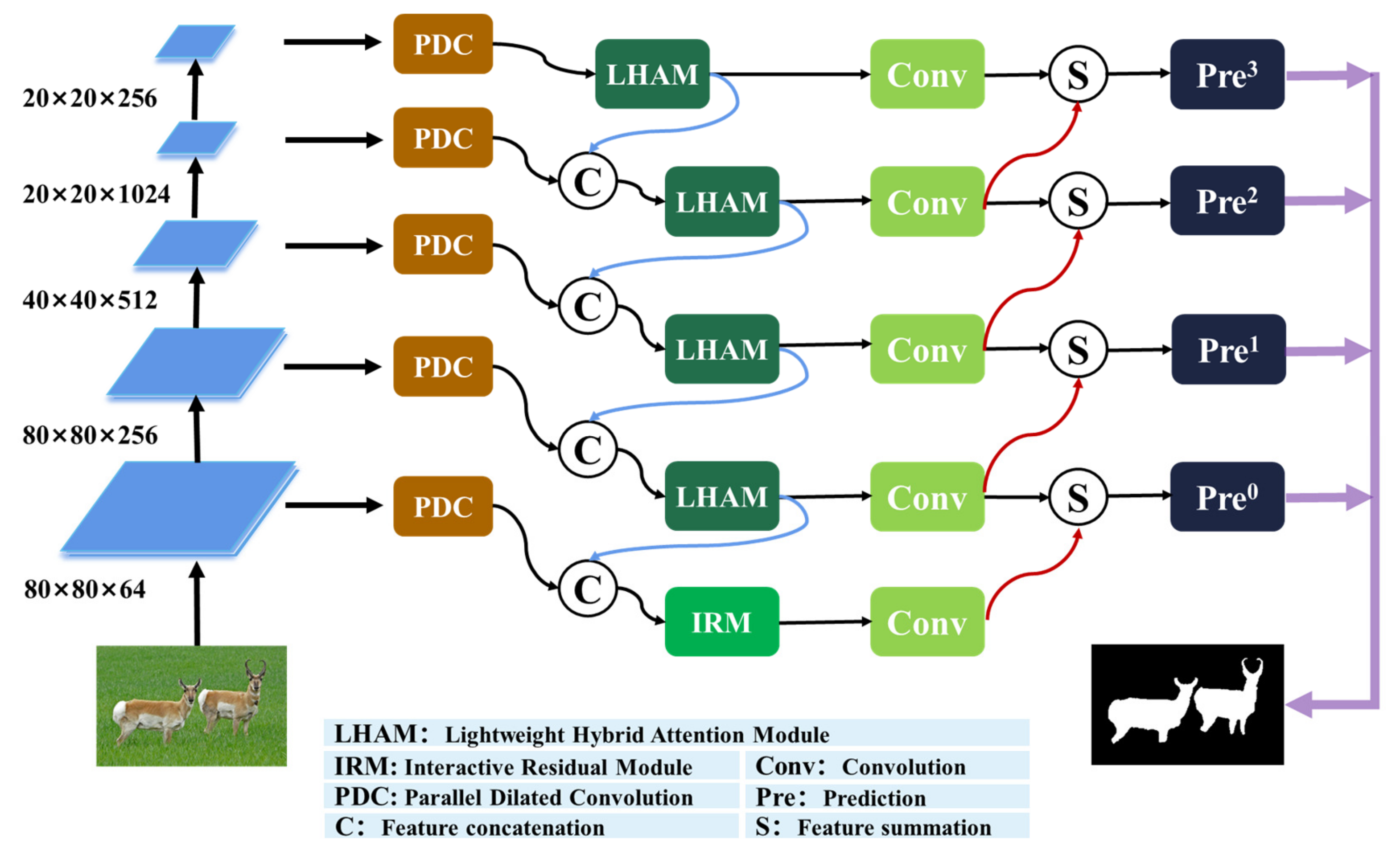
2.1. Network Framework

In this chapter, ResNet-50 is used as the backbone network in the whole model, and its side outputs are marked as {block0, block1, block2, block3, block4}. Firstly, the side outputs of the encoding network are extracted using Parallel Dilated Convolutions (PDC) with dilation rates of {1, 3, 5, 7}, and the deepest features are fed into the hybrid attention modules for high-level semantic information extraction. The extracted high-level features are fused to the output of PDC at the next layer and sent to the mixed attention module. In this way, the features fused in the direction from deep to shallow, until the second layer of the network. Then, the fused output is fed into an interactive residual network module to extract shallow features complementary to PDC. Next, we perform down-channel and up-sampling processing for each output through convolution operation and de-convolution operation, respectively, so that all outputs have the same scale. Finally, all the output features are fused according to the propagation direction from shallow to deep. The output features of each layer include fusion features and independent features, which are jointly used as the final prediction. (Note: The fusion feature refers to the feature that participates in the next level of fusion, while the independent feature is no longer involved in the fusion.) We will describe these sub-models in detail next.

2.2. Parallel Dilated Convolution

The size of the receptive field plays a decisive role in the extraction of effective features. The dilated convolution can change the size of the receptive field by changing the dilation rate while the parameters of the convolution kernel remain unchanged. In this section, the dilated convolution is adopted to extract the input information of the encoder in parallel and use the corresponding pixel addition method to fuse all the extraction results, so it is called the parallel dilated convolution module (PDC module). The schematic diagram is shown in Figure 3.

For the convenience of description, let the dilation rate be D, and each dilated convolution operation is $Con{v}^D$, and the output is F, where $I\in \{0,1,2,3,4\}$; then, the operation expression of dilated convolution is as Formula (1):

$$F_I=sum(Con{v}^D(bloc{k}^i),\dots ,Con{v}^D(bloc{k}^i)),D\in \{1,3,5,7\}$$

(1)

Among $i,I\in \{0,1,2,3,4\}$, $sum(\cdot )$ are the addition operation of the corresponding pixels of the feature. In addition, the channel must be reduced for each convolution operation. Assuming that the size of the input blockⁱ is $R^{H\times W\times C}$, the size of the output F_I is $R^{H\times W\times C/4}$.

2.3. Lightweight Hybrid Attention Module

The attention mechanism achieves the reallocation of available resources through the adjustment of weights so that salient regions get more weights, and it is commonly used in computer vision to capture deep high-level semantic information. Attention mechanism is widely used in computer vision, and it is also popular in salient detection. Among them, self-attention calculates the similarity between local features to obtain large-scale dependencies. The self-attention module is shown in Figure 4.

Specifically, the input features are linearly projected into three matrices, which are the query matrix $Q\in R^{N\times d^{\prime }}$, the key matrix $K\in R^{N\times d^{\prime }}$, and the value matrix $V\in R^{N\times d}$, respectively. The expressions of the self-attention module can be expressed as Equations (2) and (3):

$$F_O=V·soft\max (Q·K^T)$$

(2)

$$Soft\max (a_{i,j})=\frac{\exp (a_{i,j})}{{\displaystyle {\sum }_{i=1}^N\exp (a_{i,j})}}$$

(3)

Among them, N represents the number of pixels, a_i,j are the values of the corresponding pixels, d and $d^{\prime }$ represent the feature dimension, and $F_O$ represents the output. Obviously, the high computational complexity of self-attention is an obvious disadvantage. In order to reduce the exponential calculation amount of the self-attention softmax classifier, this paper will process the mapping two-dimensional matrix. First, the query matrix Q and the key matrix K are the original input feature $R^{H\times W\times C}$ to be dimensionally reduced; let $N=H\times W$, that is, each layer. The feature is the number of rows of a two-dimensional matrix, and the number of columns $d^{\prime }$ is 1/8 of the number of channels, that is, $d^{\prime }=d/8$, and d is the number of input feature channels. The number of columns of the two-dimensional matrix after the dimension reduction of the same value matrix is the number of channels of the input feature. To facilitate matrix calculation, the query matrix Q is transposed and then multiplied by the key matrix K to obtain the intermediate variable matrix $R^{N\times N}$. Then, the intermediate matrix is normalized using the softmax classification function to obtain the matrix $Z\in R^{N\times N}$, and the calculation formula is as shown in Formula (4). Finally, perform a matrix multiplication operation on the transposed matrix of the value matrix V and the matrix Z, and then perform an ascending dimension transformation on the obtained result $R^{N\times d}$. The row of the two-dimensional matrix is restored to the height and width of the feature, that is, $H\times W=N$. The calculation method is as shown in Formula (5). After the dimensionality reduction transformation, it can be obtained that the calculation amount of the classifier index operation can be changed at the cost of adding a linear interpolation. It is 1/4 of the original, and this achieves the purpose of lightweight.

$$Z=\frac{\exp (Q^T·K)}{{\displaystyle \sum \exp (Q^T·K)}}$$

(4)

$$F_S=Trans(V·Z^T)$$

(5)

In the formula, $F_S$ is the output result of spatial self-attention, and $Trans(\cdot )$ is the dimension-raising operation, so that the input and output tensors are consistent. The calculation degree of the self-attention mechanism mainly depends on the calculation amount of the index in the softmax classifier. In order to reduce the calculation amount and ensure that the features are not lost, we change the N value of the Q, K, and V matrices to 1/4 of the original, and write for $Q^{\prime }$, $K^{\prime }$, and $V^{\prime }$; then, the rows and columns of the intermediate variable matrix obtained are 1/4 of Z. After completing the calculation of $V^{\prime }$ and $Z^{\prime }$, increasing the dimension of the feature cannot reach the input tensor, so we use linear interpolation to obtain the scale of the input feature. The specific calculation process is as shown in Formula (6):

$$\{\begin{array}{l}{\tilde{F}}_S=Up(Trans(V^{\prime }·{Z^{\prime }}^T))\\ Z^{\prime }=\frac{\exp ({Q^{\prime }}^T·K^{\prime })}{{\displaystyle \sum \exp ({Q^{\prime }}^T·K^{\prime })}}\end{array}$$

(6)

where $Up(\cdot )$ is the up-sampling operation. Regarding channel orientation, we employ balanced attention to improve the interdependence between channels. The balanced attention module is to project the input feature $F\in R^{C\times H\times W}$ into a query matrix $Q\in R^{N\times C/8}$ and a key matrix $K\in R^{N\times C/8}$, where $N=H\times W$ is the number of pixels, then multiply the Q matrix and the transposed matrix of K, and use the softmax matrix to obtain the result. The function is calculated, and the result of the calculation is the degree of association between different pixels. Then, a linear layer is applied as the memory $M_v$ to share the entire dataset, and the input is fused into the above operation results to obtain the final output. The complete attention module is shown in Figure 5.

For specific details, first transform the input feature F into $\tilde{F}\in R^{C\times N}$, then multiply $\tilde{F}$ with its own transposed matrix, and send the resulting square matrix into the softmax classification function to calculate the pixel correlation in the channel direction, and then use a linear layer as a memory to transform its result into the domain $R^{C\times H\times W}$, denoting the final result by $F_C$. The whole process can be represented by Formula (7):

$$F_C=M_v·soft\max (\tilde{F}·{\tilde{F}}^T)+F$$

(7)

2.4. Asynchronous Cascading Strategy

Advanced semantic features have strong localization capabilities. To take advantage of this, we first stitch the deep features gradually to the shallow layers to complete the first step of the cascade operation. According to Figure 2, the input and output of LHAM are denoted as $F_I$ and $F_O$, respectively; then, the first cascade operation can be represented by Formula (8):

$$\{\begin{array}{l}{F}_O^i=\Gamma (F_I^i),i=0\\ F_O^i=\Gamma (Cat.(F_I^i,F_O^{i-1})),i=1,2,3\\ F_O^i={\rm I}(Cat.(F_I^i,F_O^{i-1})),i=4\end{array}$$

(8)

In the formula, the change of i from small to large represents the depth from deep to shallow, $\Gamma (\cdot )$ is the mixed attention operation, ${\rm I}(\cdot )$ is the residual interaction operation, and $Cat.(\cdot )$ is the feature splicing operation. Then, convolution and deconvolution operations are performed on the output of each layer so that the number of channels becomes 21 and all have the same size. Finally, in order to ensure that the deep features are not gradually lost in the fusion, and to improve the representation ability of the shallow features, it is necessary to carry out the second step cascade along the direction from shallow to deep. The calculation process can be expressed by Formula (9):

$$\{\begin{array}{l}{F}_{s2d}^i=sum(\mathrm{T}(Conv(F_O^i)),\mathrm{T}(Conv(F_O^{i+1}))),i=0,1,2,3\\ F_{s2d}^i=\mathrm{T}(Conv(F_O^i)),i=4\end{array}$$

(9)

Among them, $F_{s2d}$ is the final prediction result, $sum(\cdot )$ is the feature addition operation, and $Conv(\cdot )$ and $\mathrm{T}(\cdot )$ are the convolution and deconvolution operations, respectively. Figure 6 shows the feature visualization of the asynchronous cascade process, where U, C, and S represent up-sampling, channel stitching, and corresponding pixel addition fusion, respectively.

For the prediction value training, we still use the standard binary cross entropy, and the expression is as Formula (10):

$$L=-{\displaystyle \sum _{x,y}[G_{x,y}\log (P_{x,y})+(1-G_{x,y})\log (1-P_{x,y})]}$$

(10)

Among them, $G_{x,y}\in \{0,1\}$ represents the real value of the pixel $(x,y)$, and $P_{x,y}$ represents the predicted value of the pixel $(x,y)$ training. The calculation process is as Formula (11):

$$P=Sigmoid(Conv(F_{s2d}))$$

(11)

3. Experiment

3.1. Experimental Setup

Datasets. We evaluate the proposed model on six benchmark datasets: DUTS [15], ECSSD [16], PASCAL-S [17], HKU-IS [18], DUT-OMRON [19], and SOD [20]. DUTS contains 10,553 training images and 5019 testing images, and both contain complex scenes. ECSSD contains 1000 meaningful semantic images with various complex scenes. PASCAL-S contains 850 images with cluttered backgrounds and complex salient regions, all extracted from the validation set of the PASCAL VOC 2010 segmentation dataset. HKU-IS contains 4447 images with high-quality annotations, and many images have multiple disconnected salient objects. DUT-OMRON contains 5168 challenging images; most of the images in this dataset contain one or more salient objects with complex backgrounds. SOD contains 300 very challenging images, most of which contain multiple objects with low contrast or in contact with image boundaries.

Evaluation Criteria. We use three main metrics to evaluate the performance of the Hybrid Attention Asynchronous Cascade salient Detection Algorithm (HACNet) and other state-of-the-art salient object detection algorithms, including $F_{\beta }$-measure [21], Mean Absolute Error (MAE) [22], and S-measure [23]. $F_{\beta }$-measure is expressed as the weighted harmonic mean of precision and recall, and its expression is:

$$F_{\beta }=\frac{(1+{\beta }^2)Precision\times Recall}{{\beta }^2\times Precision+Recall}$$

(12)

Among them, ${\beta }^2$ is usually set to 0.3 to further emphasize the accuracy. Since the precision and recall are calculated on the basis of binary images, we first need to threshold the prediction map into a binary image. Different thresholds correspond to different $F_{\beta }$-measure. Here, we report the maximum $F_{\beta }$- measure of all thresholds. MAE is the mean absolute element-wise differences between ground truths G and predictions P, that is, to evaluate the difference between the predicted map and the ground truth map. The expression of MAE is as follows:

$$MAE=\frac{1}{W\times H}{\displaystyle \sum _{x=1}^W{\displaystyle \sum _{y=1}^H|P(x,y)-G(x,y)|}}$$

(13)

where W and H are the width and height of the image, respectively. The S-measure computes the object-aware and region-aware structural similarity between the ground truth map and the prediction map, denoted as S_o and S_r, which is expressed as:

$$S=\gamma ·S_o+(1-\gamma )·S_r$$

(14)

where $\gamma$ is set to 0.5.

Implementation Details. We implement our proposed model based on the Pytorch framework. To facilitate comparison with other works, we choose ResNet-50 [24] as the skeleton network. Following most existing methods, we use the DUTS-TR dataset as the training set and the SOD dataset as the validation set to update the weights. Our network is based on NVIDIA GTX 1080 Ti GPU, and the operating system is Ubuntu 16.04 for training. To ensure model convergence, we use the Adam [25] optimizer to train our model with learning rate set to 8e-5, batch size set to 8, and resolution adjusted to $320\times 320$. During the entire training period, the model is trained for about 15 h and converged after 15 epochs.

3.2. Ablation Experiment

In this section, we mainly study the effectiveness of parallel dilated convolution, lightweight hybrid attention module, and asynchronous cascade fusion strategy. The effectiveness test of each step is based on the data of the DUTS-TE test set. The experimental arrangement is shown in

Table 1. Ablation experiments based on DUTS-TE dataset. The best results are shown in bold face. ↑ and ↓ indicate that the larger and smaller scores are better, respectively.

Model	F-Measure ↑	MAE ↓	S-Measure ↑
ResNet	0.709	0.077	0.777
ResNet + PDC	0.739	0.075	0.801
ResNet + LHAM	0.745	0.071	0.806
ResNet + BACS	0.741	0.072	0.803
ResNet + PDC + LHAM	0.782	0.058	0.828
ResNet + PDC + BACS	0.759	0.065	0.814
ResNet + LHAM + BACS	0.785	0.057	0.830
ResNet + PDC + LHAM + BACS	0.800	0.053	0.840

Note: PDC stands for parallel dilated convolution, LHAM stands for Lightweight hybrid attention module, and BACS stands for Asynchronous Cascading Strategy.

, and the optimal data has been marked in bold.

3.2.1. Effectiveness Experiment of PDC

PDC changes the size of the receptive field by changing the dilation rate without changing the parameters of the convolution kernel. The size of the receptive field determines the effect of feature extraction. In order to determine the best combination of dilated convolutions, we first test the number of dilated convolutions k under the condition that the dilation rate is 1. Since PDC is only applied to the side output, additional down-channeling and up-sampling are required after the PDC output. The experiments are carried out for four different k values, 2, 3, 4, 5, and the DUTS-TE test results are recorded in

Table 2. Evaluating the number of dilated convolutions on the DUTS-TE dataset. (The best results are shown in bold face. ↑ and ↓ indicate that the larger and smaller scores are better, respectively.)

k	F-Measure ↑	MAE ↓	S-Measure ↑
2	0.435	0.282	0.548
3	0.442	0.279	0.551
4	0.448	0.270	0.558
5	0.447	0.270	0.556

.

According to Table 2, it can be found that when k = 4, the effect is the best, so we test the dilation rate under the condition that the number of PDCs is four, mainly in five different situations, namely {1, 1, 1, 1}, {1,2,3,4}, {1,2,4,5}, {1,3,5,7}, {1,4,5,6}. We record the dilation rate results in

Table 3. Evaluation on the DUTS-TE dataset with different dilation rates. (The best results are shown in bold face. ↑ and ↓ indicate that the larger and smaller scores are better, respectively.)

No.	F-Measure ↑	MAE ↓	S-Measure ↑
{1,1,1,1}	0.448	0.270	0.558
{1,2,3,4}	0.482	0.217	0.598
{1,2,4,5}	0.502	0.212	0.611
{1,3,5,7}	0.512	0.200	0.619
{1,4,5,6}	0.506	0.217	0.610

; according to the results in the table, the detection effect is the best when the dilation rate is {1, 3, 5, 7}. The validity experiment of PDC is different from the test of only the backbone network. The test of the backbone network only uses the output of the last layer as the output result. Similarly, the Res + PDC in Table 1 is also a PDC module added only in the last layer. The effectiveness experiment of PDC is to evaluate the side output of different depths. In addition, it can be seen that the performance after adding PDC is obviously better than the performance of the backbone network itself.

3.2.2. Effectiveness Experiments of LHAM and BACS

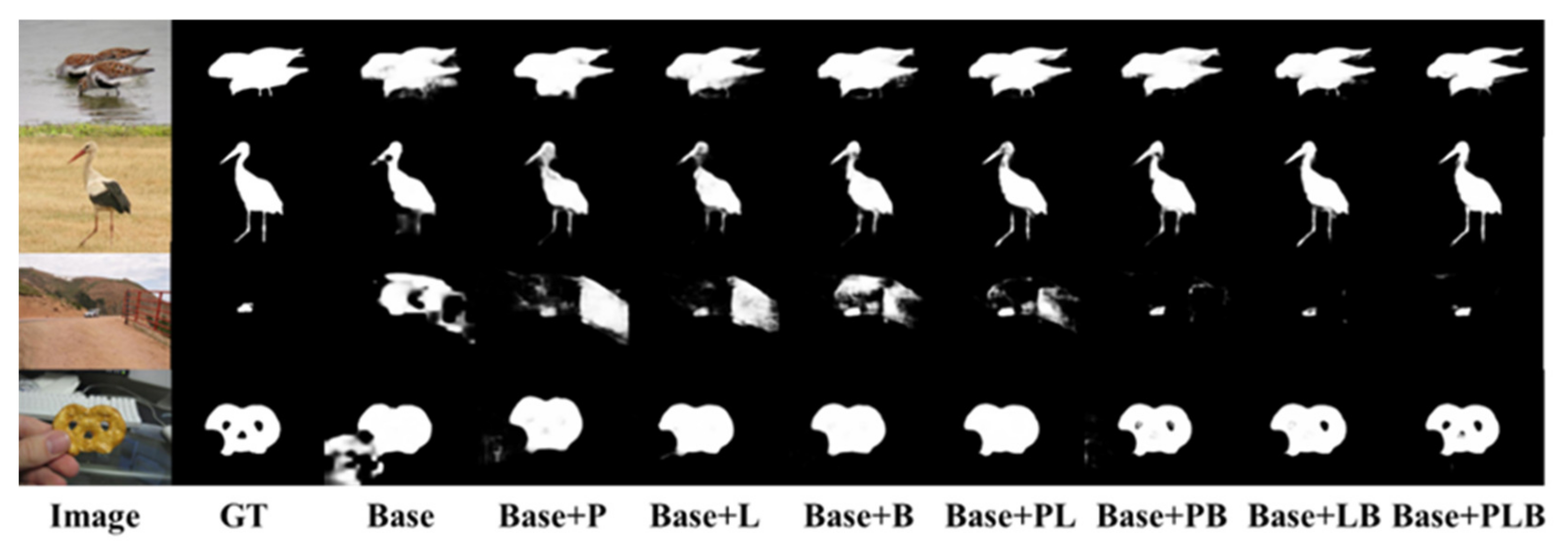
LHAM mainly includes a lightweight self-attention module based on spatial orientation and a balanced attention module based on channel orientation. Because the computational complexity of reducing self-attention in the spatial direction is more obvious, and the computational complexity of balancing attention itself is also lower than that of self-attention, the lightweight self-attention is only used for feature extraction in the spatial direction. It can be found in Table 1 that the detection performance is greatly improved by using LHAM. For BACS, we first test the performance of each output working independently, that is, ResNet + PDC + LHAM in Table 1, and then evaluate by gradually adding cascade operations. Through deep-to-shallow and shallow-to-deep feature fusion, we can find that the detection performance has been improved. We do not show the specific details, but the final detection effect is recorded in Table 1. Figure 7 shows that the partial ablation is an experimental effect diagram. From the figure, each module can play a complementary role. For example, in the third picture, a small object is used as the foreground, and the salient position is accurately located by gradually filtering the background.

3.3. Comparison with State-of-the-Art

In this section, we compare HACNet with 14 other state-of-the-art salient detection methods, including Amulet [10], MDF [18], MBINet [14], LEGS [26], MCDL [27], ELD [28], DCL [29], DSS [30], CANet [31], NLDF [32], UCF [33], RFCN [34], BSCA [35], and RSD [36]. For fair comparison, the prediction maps of the above methods are provided by the authors or calculated by running the source code.

3.3.1. Quantitative Comparison

We evaluate the proposed method in terms of F-measure, MAE, and S-measure, and also compare it with other salient object detection methods, and the results have been recorded in

Table 4. Quantitative evaluation of different salient detection methods on five benchmark datasets. (The best results are shown in bold face. ↑ and ↓ indicate that the larger and smaller scores are better, respectively).

Model	DUTS-TE			ECSSD			PASCAL-S			HKU-IS			DUT-OMROM
	F ↑	M ↓	S ↑	F ↑	M ↓	S ↑	F ↑	M ↓	S ↑	F ↑	M ↓	S ↑	F ↑	M ↓	S ↑
Ours	0.800	0.053	0.840	0.900	0.051	0.890	0.800	0.085	0.813	0.900	0.039	0.890	0.725	0.058	0.804
MBI [14]	0.809	0.058	0.824	0.909	0.058	0.886	0.821	0.092	0.806	0.901	0.042	0.880	0.763	0.069	0.781
CANet [31]	0.796	0.056	0.840	0.907	0.049	0.898	0.832	0.120	0.790	0.897	0.040	0.895	0.719	0.071	0.795
NLDF [32]	0.813	0.065	0.816	0.905	0.063	0.875	0.822	0.098	0.805	0.902	0.048	0.878	0.753	0.080	0.771
Amulet [10]	0.773	0.075	0.796	0.911	0.062	0.849	0.862	0.092	0.820	0.889	0.052	0.886	0.737	0.083	0.771
DCL [29]	0.782	0.088	0.795	0.891	0.088	0.863	0.804	0.124	0.791	0.885	0.072	0.861	0.739	0.097	0.764
UCF [33]	0.771	0.116	0.777	0.908	0.080	0.884	0.820	0.127	0.806	0.888	0.073	0.874	0.735	0.131	0.748
DSS [30]	0.813	0.065	0.812	0.906	0.064	0.882	0.821	0.101	0.796	0.900	0.050	0.878	0.760	0.074	0.765
ELD [28]	0.747	0.092	0.749	0.865	0.082	0.839	0.772	0.122	0.757	0.843	0.072	0.823	0.738	0.093	0.743
RFCN [34]	0.784	0.091	0.791	0.898	0.097	0.860	0.827	0.118	0.793	0.895	0.079	0.859	0.747	0.095	0.774
BSCA [35]	0.597	0.197	0.630	0.758	0.183	0.725	0.666	0.224	0.633	0.723	0.174	0.700	0.616	0.191	0.652
MDF [18]	0.729	0.093	0.732	0.832	0.105	0.776	0.763	0.143	0.694	0.860	0.129	0.810	0.694	0.092	0.720
RSD [36]	0.757	0.161	0.724	0.845	0.173	0.788	0.864	0.155	0.805	0.843	0.156	0.787	0.633	0.178	0.644
LEGS [26]	0.655	0.138	-	0.827	0.118	0.787	0.756	0.157	0.682	0.770	0.118	-	0.669	0.133	-
MCDL [27]	0.461	0.276	0.545	0.837	0.101	0.803	0.741	0.143	0.721	0.808	0.092	0.786	0.701	0.089	0.752

. As can be seen from the results, our method significantly outperforms most other salient detection methods. In particular, the MAE data is optimal on the DUT-TE, PASCAL-S, HKU-IS, and DUT-OMROM datasets.

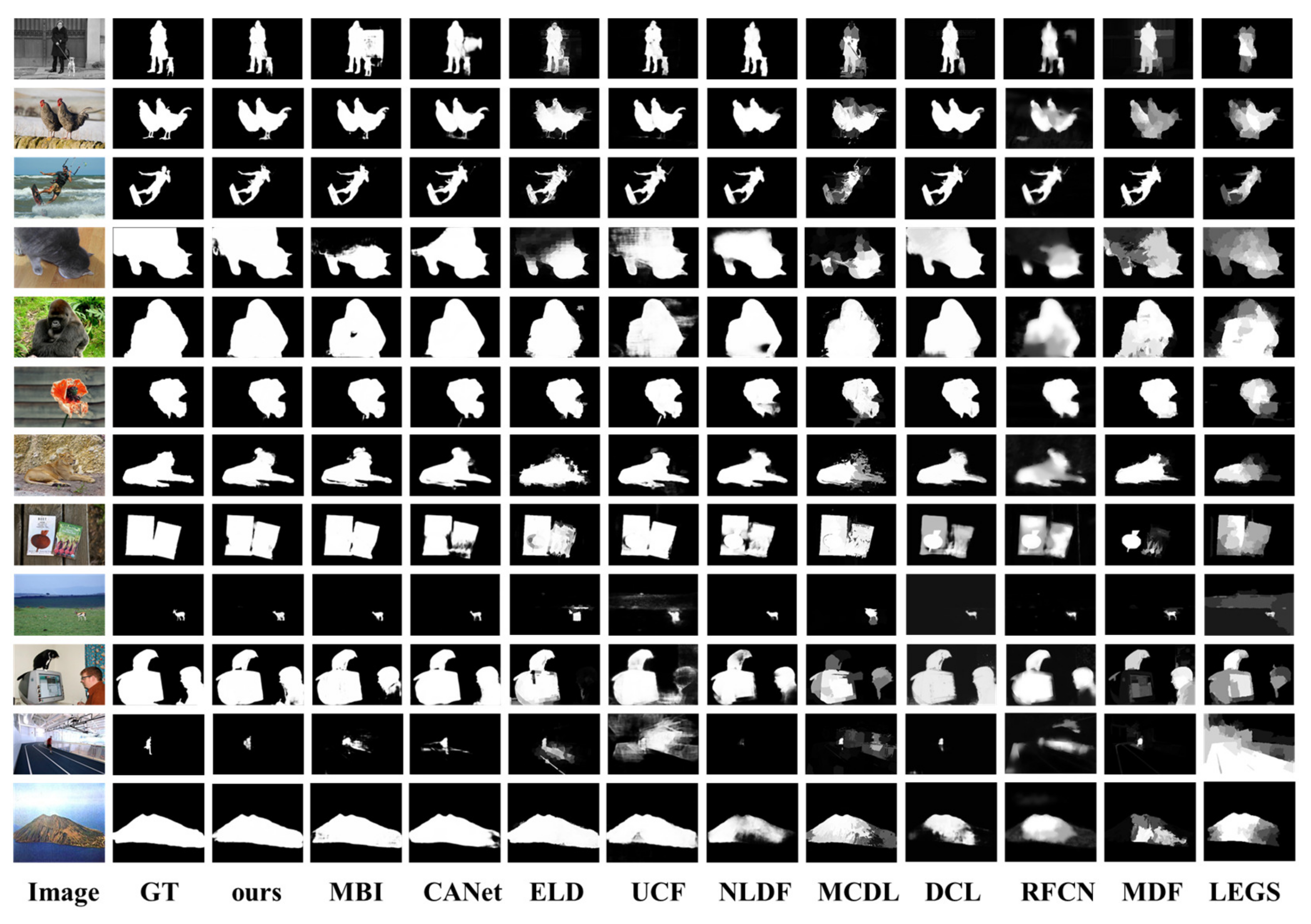
3.3.2. Qualitative Comparison

Figure 8 shows the detection performance of some different test sets. The first picture shows two adjacent salient regions, and it can be found that this method is more accurate for the detection of puppies. The fourth and fifth pictures show the detection effect of large features, while the ninth picture is the detection effect of small features. The contrast between the foreground and background of the seventh image is low, so there are still errors in the detection of partial detail areas. The 10th picture shows the detection effect of the coexistence of multiple salient objects, and it can be found that the detection effect of this method is closer to the ground truth map.

4. Conclusions

In this paper, HACNet is proposed to improve the performance of salient object detection, which mainly solves the problem of effective fusion of features in different depths. First, we employ parallel dilated convolution (PDC) to extract the features on the side outputs of the backbone network ResNet-50. Then, the extracted features are fed into our improved lightweight hybrid attention module (LHAM) using a feedback mechanism gradually from deep to shallow to improve the localization ability of high-level semantic features. When feeding back to the shallowest layer, we replace the mixed attention module with an interactive residual network to process detailed features and complete the first cascade operation. Next, a convolution operation is performed on the output of each layer to unify the number of channels. Finally, through the process of gradually up-sampling the feature parameters and fusing the feature parameters, the shallow detail features can be better represented in the saliency map. At the same time, through the above operations, the second cascade operation is completed, and each fusion result is taken as the final prediction value. The experimental results of the five benchmark datasets show that the proposed model can predict the salient regions with high accuracy.

However, HACNet still has problems, such as a more complex network structure and larger number of model parameters. In the future research work, we will further optimize the network architecture and improve the generalization and robustness of the salient object detection algorithm to meet more scenario requirements.

References

- Cheng, X.; Li, E.; Fu, Z. Residual Attention Siamese RPN for Visual Tracking. In Proceedings of the Chinese Conference on Pattern Recognition and Computer Vision (PRCV), Nanjing, China, 16–18 October 2020. [Google Scholar]
- Mehta, D.; Skliar, A.; Yahia, H.B.; Borse, S.; Porikli, F.M. Simple and Efficient Architectures for Semantic Segmentation. In Proceedings of the 2022 IEEE/CVF Conference on Computer Vision and Pattern Recognition Workshops (CVPRW), New Orleans, LA, USA, 19–20 June 2022; pp. 2627–2635. [Google Scholar]
- Zhou, Z.; Pei, X.; Li, X.; Wang, H.; Zheng, F.; He, Z. Saliency-associated object tracking. In Proceedings of the IEEE/CVF International Conference on Computer Vision, Montreal, BC, Canada, 11–17 October 2021; pp. 9866–9875. [Google Scholar]
- Qin, X.; Zhang, Z.; Huang, C.; Dehghan, M.; Zaiane, O.R.; Jägersand, M. U2-Net: Going Deeper with Nested U-Structure for Salient Object Detection. Pattern Recognit 2020, 106, 107404. [Google Scholar] [CrossRef]
- Yang, C.; Zhang, L. Saliency detection via graph-based manifold ranking. IEEE Trans. Multim. 2020, 22, 885–896. [Google Scholar]
- Borji, A.; Cheng, M.; Jiang, H.; Li, J. Salient object detection: A survey. Comput. Vis. Media 2014, 5, 117–150. [Google Scholar] [CrossRef] [Green Version]
- Li, X.; Lu, H.; Zhang, L. Saliency detection via dense and sparse reconstruction. In Proceedings of the IEEE International Conference on Computer Vision, Sydney, Australia, 1–8 December 2013; pp. 2976–2983. [Google Scholar]
- Sun, L.; Chen, Z.; Wu, Q.J.; Zhao, H.; He, W.; Yan, X. AMPNet: Average-and Max-Pool Networks for Salient Object Detection. IEEE Trans. Circuits Syst. Video Technol. 2021, 31, 4321–4333. [Google Scholar] [CrossRef]
- Yun, Y.; Lin, W. SelfReformer: Self-Refined Network with Transformer for Salient Object Detection. arXiv 2022, arXiv:2205.11283. [Google Scholar]
- Zhang, P.; Wang, D.; Lu, H.; Wang, H.; Ruan, X. Amulet: Aggregating multi-level convolutional features for salient object detection. In Proceedings of the 16th IEEE International Conference on Computer Vision (ICCV), Venice, Italy, 22–29 October 2017; pp. 202–211. [Google Scholar]
- He, J.; Zhang, S.; Yang, M.; Shan, Y.; Huang, T. Bdcn: Bi-directional cascade network for perceptual edge detection. IEEE Trans. Pattern Anal. Mach. Intell. 2020, 44, 100–113. [Google Scholar] [CrossRef] [PubMed]
- Vaswani, A.; Shazeer, N.; Parmar, N.; Uszkoreit, J.; Jones, L.; Gomez, A.N.; Kaiser, L.; Polosukhin, I. Attention is all you need. In Proceedings of the Advances in Neural Information Processing Systems (NIPS), Long Beach, CA, USA, 4 December 2017. [Google Scholar]
- Guo, M.H.; Liu, Z.N.; Mu, T.J.; Hu, S.M. Beyond self-attention: External attention using two linear layers for visual tasks. arXiv 2021, arXiv:2105.02358. [Google Scholar] [CrossRef] [PubMed]
- Yang, H.; Chen, R.; Deng, D. Multiscale Balanced-Attention Interactive Network for Salient Object Detection. Mathematics 2022, 10, 512. [Google Scholar] [CrossRef]
- Wang, L.; Lu, H.; Wang, Y.; Feng, M.; Wang, D.; Yin, B.; Ruan, X. Learning to detect salient objects with image-level supervision. In Proceedings of the IEEE Conference on Computer Vision and Pattern Recognition, Honolulu, HI, USA, 21–26 July 2017; pp. 136–145. [Google Scholar]
- Yan, Q.; Xu, L.; Shi, J.; Jia, J. Hierarchical saliency detection. In Proceedings of the IEEE Conference on Computer Vision and Pattern Recognition, Portland, OR, USA, 23–28 June 2013; pp. 1155–1162. [Google Scholar]
- Li, Y.; Hou, X.; Koch, C.; Rehg, J.M.; Yuille, A.L. The secrets of salient object segmentation. In Proceedings of the IEEE Conference on Computer Vision and Pattern Recognition, Columbus, OH, USA, 23–28 June 2014; pp. 280–287. [Google Scholar]
- Li, G.; Yu, Y. Visual saliency based on multiscale deep features. In Proceedings of the IEEE Conference on Computer Vision and Pattern Recognition, Boston, MA, USA, 7–12 July 2015; pp. 5455–5463. [Google Scholar]
- Yang, C.; Zhang, L.; Lu, H.; Ruan, X.; Yang, M.H. Saliency detection via graph-based manifold ranking. In Proceedings of the IEEE Conference on Computer Vision and Pattern Recognition, Portland, OR, USA, 23–28 July 2013; pp. 3166–3173. [Google Scholar]
- Movahedi, V.; Elder, J.H. Design and perceptual validation of performance measures for salient object segmentation. In Proceedings of the 2010 IEEE Computer Society Conference on Computer Vision and Pattern Recognition-Wor, San Francisco, CA, USA, 13–18 June 2010; pp. 49–56. [Google Scholar]
- Achanta, R.; Hemami, S.; Estrada, F.; Susstrunk, S. Frequency-tuned salient region detection. In Proceedings of the IEEE Conference on Computer vision and Pattern Recognition, Miami, FL, USA, 20–25 June 2009; pp. 1597–1604. [Google Scholar]
- Perazzi, F.; Krähenbühl, P.; Pritch, Y.; Hornung, A. Saliency filters: Contrast based filtering for salient region detection. In Proceedings of the 2012 IEEE Conference on Computer Vision and Pattern Recognition, Providence, RI, USA, 16–21 June 2012; pp. 733–740. [Google Scholar]
- Fan, D.P.; Cheng, M.M.; Liu, Y.; Li, T.; Borji, A. Structure-measure: A new way to evaluate foreground maps. In Proceedings of the IEEE International Conference on Computer Vision, Honolulu, HI, USA, 21–26 July 2017; pp. 4548–4557. [Google Scholar]
- He, K.; Zhang, X.; Ren, S.; Sun, J. Deep residual learning for image recognition. In Proceedings of the 2016 IEEE Conference on Computer Vision and Pattern Recognition (CVPR), Seattle, WA, USA, 27–30 June 2016; pp. 770–778. [Google Scholar]
- Kingma, D.P.; Ba, J. Adam: A method for stochastic optimization. arXiv 2014, arXiv:1412.6980. [Google Scholar]
- Wang, L.; Lu, H.; Ruan, X.; Yang, M.H. Deep Networks for Saliency Detection via Local Estimation and Global Search. In Proceedings of the 2015 IEEE Conference on Computer Vision and Pattern Recognition (CVPR), Boston, MA, USA, 7–12 June 2015; pp. 3183–3192. [Google Scholar]
- Zhao, R.; Ouyang, W.; Li, H.; Wang, X. Saliency Detection by Multi-context Deep Learning. In Proceedings of the 2015 IEEE Conference on Computer Vision and Pattern Recognition (CVPR), Boston, MA, USA, 7–12 June 2015; pp. 1265–1274. [Google Scholar]
- Lee, G.; Tai, Y.W.; Kim, J. Deep saliency with encoded low level distance map and high level features. In Proceedings of the 2016 IEEE Conference on Computer Vision and Pattern Recognition (CVPR), Seattle, WA, USA, 27–30 June 2016; pp. 660–668. [Google Scholar]
- Li, G.; Yu, Y. Deep contrast learning for salient object detection. In Proceedings of the 2016 IEEE Conference on Computer Vision and Pattern Recognition (CVPR), Seattle, WA, USA, 27–30 June 2016; pp. 478–487. [Google Scholar]
- Hou, Q.B.; Cheng, M.M.; Hu, X.W.; Borji, A.; Tu, Z.; Torr, P. Deeply Supervised Salient Object Detection with Short Connections. IEEE Trans. Pattern Anal. Mach. Intell. 2019, 41, 815–828. [Google Scholar] [CrossRef] [PubMed] [Green Version]
- Li, J.; Pan, Z.; Liu, Q.; Cui, Y.; Sun, Y. Complementarity-Aware Attention Network for Salient Object Detection. IEEE Trans. Cybern. 2020, 52, 873–886. [Google Scholar] [CrossRef] [PubMed]
- Luo, Z.; Mishra, A.; Achkar, A.; Cui, Y.; Sun, Y. Non-local deep features for salient object detection. In Proceedings of the 2017 IEEE Conference on Computer Vision and Pattern Recognition (CVPR), Honolulu, HI, USA, 21–26 June 2017; pp. 6609–6617. [Google Scholar]
- Zhang, P.; Wang, D.; Lu, H.; Wang, H.; Yin, B. Learning uncertain convolutional features for accurate saliency detection. In Proceedings of the 16th IEEE International Conference on Computer Vision (ICCV), Venice, Italy, 22–29 October 2017; pp. 212–221. [Google Scholar]
- Wang, L.; Wang, L.; Lu, H.; Zhang, P.; Ruan, X. Salient object detection with recurrent fully convolutional networks. IEEE Trans. Pattern Anal. Mach. Intell. 2018, 41, 1734–1746. [Google Scholar] [CrossRef] [PubMed]
- Qin, Y.; Lu, H.; Xu, Y.; Wang, H. Saliency detection via cellular automata. In Proceedings of the 2015 IEEE Conference on Computer Vision and Pattern Recognition (CVPR), Boston, MA, USA, 7–12 June 2015; pp. 110–119. [Google Scholar]
- Islam, M.A.; Kalash, M. Revisiting salient object detection: Simultaneous detection, ranking, and subitizing of multiple salient objects. In Proceedings of the 2018 IEEE Conference on Computer Vision and Pattern Recognition, Salt Lake City, UT, USA, 18–23 June 2018; pp. 7142–7150. [Google Scholar]
Figure 1.
Complete flowchart of HACNet.
Figure 2.
Schematic diagram of the structure of HACNet.
Figure 3.
Schematic diagram of the structure of parallel dilated convolution.
Figure 4.
Self-attention module.