Integration of Differential Equations by ${\mathcal{C}}^{\mathbf{\infty }}$-Structures

Abstract

Several integrability problems of differential equations are addressed using the concept of a ${\mathcal{C}}^{\infty }$-structure, a recent generalization of the notion of solvable structure. Specifically, the integration procedure associated with ${\mathcal{C}}^{\infty }$-structures is used to integrate a Lotka–Volterra model and several differential equations that lack sufficient Lie point symmetries and cannot be solved using conventional methods.

1. Introduction

Solvable structures appeared in the last decade of the 20th century as a generalization of the concept of solvable symmetry algebra [1,2,3,4], in order to characterize the integrability by quadratures of an involutive distribution of vector fields $\mathcal{Ƶ}$ on a n-dimensional manifold [5,6,7,8]. Roughly speaking, a solvable structure for a distribution $\mathcal{Ƶ}$ of rank r consists of a sequence of $n-r$ vector fields that gives rise to a chain of distributions such that each vector field in the structure is a symmetry of the previous distribution.

Almost at the same time, ${\mathcal{C}}^{\infty }$-symmetries were introduced as a generalization of the classical Lie symmetry method of reduction [1,2] for ordinary differential equations (ODEs) [9]. Since their introduction, ${\mathcal{C}}^{\infty }$-symmetries have been extended in multiple directions [10,11,12,13,14,15,16,17,18,19,20,21,22,23,24,25]. They are being extensively used [26,27,28,29,30,31,32,33,34,35,36,37,38,39], allowing to solve equations that may even lack Lie point symmetries [9,40,41].

The idea that allowed extending the notion of Lie point symmetry to ${\mathcal{C}}^{\infty }$-symmetry, in the context of ODEs, has been adapted in [42,43] for involutive distributions of vector fields. The condition for a vector field to be a ${\mathcal{C}}^{\infty }$-symmetry of a distribution is less restrictive than for a symmetry, which implies that in practice the ${\mathcal{C}}^{\infty }$-symmetries of a distribution are easier to find than its symmetries. When considering the notion of a solvable structure, we let the elements be ${\mathcal{C}}^{\infty }$-symmetries, instead of symmetries, of the chains of distributions mentioned above, and we obtain a more general structure, which has been called a ${\mathcal{C}}^{\infty }$-structure in [42]. The key point in this new theory is that once a ${\mathcal{C}}^{\infty }$-structure for an involutive distribution $\mathcal{Ƶ}$ of corank k has been determined, then $\mathcal{Ƶ}$ can be integrated by sequentially solving k integrable Pfaffian equations ([42] Theorem 3.5). These Pfaffian equations are defined in spaces whose dimensions decrease one unit at each stage. The Pfaffian equations are completely integrable, although, unlike solvable structures, they may not be integrable by quadratures. The well known outcome relating integrating factors and Lie point symmetries for first-order ODEs [1,3,4,44] has been recently extended in [43]. The extension applies to ${\mathcal{C}}^{\infty }$-structures and involutive distributions of arbitrary corank by introducing symmetrizing factors. Relevant results on the role played by these symmetrizing factors on the integrability by quadratures of the Pfaffian equations arising by the application of the ${\mathcal{C}}^{\infty }$-structure method have been also derived [43].

In this work, we present some new applications of the integration procedure associated with ${\mathcal{C}}^{\infty }$-structures. The paper is organized as follows: in Section 2 and Section 3 we recall the main definitions and results in the theory of ${\mathcal{C}}^{\infty }$-structures, by adapting some of the theoretical results that were obtained in [42] to the problems that we address in this paper. In Section 4, we explore the application of the ${\mathcal{C}}^{\infty }$-structure method to fully integrate two systems of first-order ordinary differential equations, one of which is a Lotka–Volterra system, frequently used to describe the dynamics of biological systems. Additionally, we investigate three scalar ODEs in Section 5, two of which are of the fourth order and one of the third order. Notably, the considered equations exhibit a lack of sufficient Lie point symmetries, and even powerful symbolic systems like Maple fail to provide explicit solutions for them. Nevertheless, our novel integration method based on ${\mathcal{C}}^{\infty }$-structures leads to the complete integration of equations that are difficult to solve using conventional methods.

2. Preliminaries

In this paper, we consider all functions, vector fields, and differential forms to be smooth (meaning ${\mathcal{C}}^{\infty }$) within a contractible open subset U of ${\mathbb{R}}^n.$ In what follows, $\mathfrak{X}\left(U\right)$ and ${\Omega }^k\left(U\right)$ are used to represent the ${\mathcal{C}}^{\infty }\left(U\right)$-module of all smooth vector fields and k-forms, respectively, whereas ${\Omega }^{*}\left(U\right)$ stands for the algebra of exterior differentials encompassing all differential forms on U.

Given a set $\{{\mathcal{Z}}_1,\dots ,{\mathcal{Z}}_r\}$ of pointwise linearly independent vector fields on $U,$ by $\mathcal{Ƶ}:=S\left(\{{\mathcal{Z}}_1,\dots ,{\mathcal{Z}}_r\}\right)$ we denote the submodule of $\mathfrak{X}\left(U\right)$ generated by $\{{\mathcal{Z}}_1,\dots ,{\mathcal{Z}}_r\}.$ In a similar way, the submodule of ${\Omega }^1\left(U\right)$ generated by a set of pointwise linearly independent 1-forms $\{{\sigma }_1,\dots ,{\sigma }_s\}$ will be denoted by $\mathcal{P}:=S\left(\{{\sigma }_1,\dots ,{\sigma }_s\}\right).$ The submodule $\mathcal{Z}$ (resp. $\mathcal{P}$) defines a distribution (resp. a Pfaffian system) of constant rank $n-r$ (resp. $n-s$).

The annihilator of $\mathcal{Ƶ}$ is the set of the differential forms $\omega \in {\Omega }^{*}\left(U\right)$ such that $\omega (Y_1,\dots ,Y_k)=0$ whenever $Y_1,\dots ,Y_k\in \mathcal{Ƶ}.$ This set, which will be denoted by $Ann\left(\mathcal{Ƶ}\right),$ is an ideal of ${\Omega }^{*}\left(U\right)$ locally generated by $n-r$ pointwise linearly independent 1-forms $\{{\omega }_1,\dots ,{\omega }_{n-r}\}$ [45,46]. In this case, we will write ${\mathcal{Ƶ}}^{\circ }=S\left(\{{\omega }_1,\dots ,{\omega }_{n-r}\}\right).$ It can be checked that the Pfaffian system ${\mathcal{Ƶ}}^{\circ }$ can be characterized in terms of the interior product [46] or contraction ⨼ as follows:

$${\mathcal{Ƶ}}^{\circ }=\{\omega \in {\Omega }^1\left(U\right):\mathcal{Z}⨼\omega =0,\mathrm{for} \mathrm{each}\mathcal{Z}\in \mathcal{Ƶ}\}.$$

Let us recall that the distribution $\mathcal{Ƶ}$ is said to be involutive if $[{\mathcal{Z}}_i,{\mathcal{Z}}_j]\in \mathcal{Ƶ}$ for $1\le i, j\le r.$ A well-known result states that $\mathcal{Ƶ}$ is involutive if and only if the ideal $\mathrm{Ann}\left(\mathcal{Ƶ}\right)$ is closed under exterior differentiation $d$, i.e. if $\mathrm{Ann}\left(\mathcal{Ƶ}\right)$ is a differential ideal (see, for instance, Proposition 2.30 and Definition 2.29 in [45]). In this case, Frobenius Theorem ([45] Theorem 1.60) guarantees that, for each $p\in U,$ the local existence of a unique connected integral manifold of $\mathcal{Ƶ}$ of maximal dimension ([45] Definition 1.63). Such integral manifolds can be defined (locally) by the level sets of a complete set of first integrals $I_1,\dots ,I_{n-r}$ for the distribution $\mathcal{Ƶ}.$ It is clear that, in this case, the independent 1-forms $\{d{I}_1,\dots ,d{I}_{n-r}\}$ generate the corresponding Pfaffian system ${\mathcal{Ƶ}}^{\circ },$ which is said to be completely integrable [45,46]. In this sense, integrating a completely integrable Pfaffian system is equivalent to integrating the corresponding involutive system of vector fields.

In such integration procedures, the notion of solvable structure, introduced by Basarab-Horwath in [5], plays a fundamental role (see also [7]). This concept is based on the notion of symmetry of a distribution, which generalizes Lie point symmetries: [5,47,48]:

Definition 1.

A symmetry of an involutive distribution $\mathcal{Ƶ}$ is a vector field X such that the set $\{{\mathcal{Z}}_1,\dots ,{\mathcal{Z}}_r,X\}$ is pointwise linearly independent on U and $[X,\mathcal{Ƶ}]\subset \mathcal{Ƶ}$.

Now we can recall the concept of solvable structure:

Definition 2

([5] Definiton 4). A solvable structure for $\mathcal{Ƶ}$ consists of an ordered set of vector fields $\langle X_1,\dots ,X_{n-r}\rangle$ such that $X_1$ is a symmetry of $\mathcal{Ƶ}$ and $X_i$ is a symmetry of the distribution $\mathcal{Ƶ}\oplus S\left(\{X_1,\dots ,X_{i-1}\}\right)$ for $i=2,\dots ,n-r.$

The main result concerning solvable structures is that the knowledge of a solvable structure allows us to find the integral manifolds of $\mathcal{Ƶ}$, at least locally, by quadratures alone ([5] Proposition 3). A dual version of Definition 2, given in terms of differential 1-forms, was introduced in ([6] Defintion 4) by Hartl and Athorne. These authors also re-established the integrability result by Basarab-Horwath from a dual point of view (see [6] Proposition 5). We refer the reader also to [8,49,50] for further details on the integration procedure associated with solvable structures.

Solvable structures are very useful in the study of ordinary differential equations (ODEs), because such problems can be reformulated as the task of integrating systems of vector fields or 1-forms. For instance, consider a system of first-order ODEs

$$\left\{\begin{array}{ccc}{\dot{x}}_1\hfill & =& {\varphi }_1(t,x_1,\dots ,x_n),\hfill \\ {\dot{x}}_2\hfill & =& {\varphi }_2(t,x_1,\dots ,x_n),\hfill \\ \hfill & ⋮& \\ {\dot{x}}_n\hfill & =& {\varphi }_n(t,x_1,\dots ,x_n),\hfill \end{array}\right.$$

(1)

where ${\varphi }_1,\dots ,{\varphi }_n$ are smooth functions on some open set $U\subset {\mathbb{R}}^{n+1}$ and over dot denotes differentiation with respect to the independent variable $t.$ Any solution of system (1) defines a one-dimensional integral manifold of the (trivially involutive) rank 1 distribution generated by the vector field

$$\mathcal{Z}={\partial }_t+{\varphi }_1(t,x_1,\dots ,x_n){\partial }_{x_1}+\dots +{\varphi }_n(t,x_1,\dots ,x_n){\partial }_{x_n}.$$

(2)

The extension to systems of ODEs of higher order is straightforward. Consider, for instance, a general mth-order ODE:

$$u_m=\varphi (x,u^{(m-1)}),$$

(3)

where $u^{(m-1)}=(u,u_1,\dots ,u_{m-1})$ denotes the dependent variable u and, for $1\le k\le m,$ $u_k$ denotes the derivative of order k of u with respect to the independent variable $x.$ By setting $x=t,$ $x_1=u,$ and $x_k=u_{k-1},$ for $1\le k\le m,$ then Equation (3) can be transformed into a system of the form (1), whose associated vector field (2), written in terms of original variables $(x,u^{(m-1)}),$ becomes

$$\mathcal{Z}={\partial }_x+u_1{\partial }_u+\dots +\varphi (x,u^{(m-1)}){\partial }_{u_{m-1}}.$$

(4)

In this case, any integral manifold of the distribution generated by the vector field (4) corresponds to the $(m-1)$th-prolongation of a solution of Equation (3) [1,3,4].

Therefore, the method of solvable structures can be applied to integrate the given ODE (or the system of ODEs) by quadratures alone. This outcome extends the classical result stating that a system of m differential equations of order n, accompanied by a solvable Lie point symmetry algebra of dimension $mn$, can be solved using quadratures. We refer the reader to ([6] Proposition 6) and ([7] Section V) for further details on the application of solvable structures to the integration of differential equations.

3. ${\mathcal{C}}^{\mathbf{\infty }}$-Structures and Integrability of Distributions

This notion of ${\mathcal{C}}^{\infty }$-symmetry for a distribution was introduced in ([42] Definition 3.2), as a generalization of the idea of ${\mathcal{C}}^{\infty }$-symmetry for ODEs [9]:

Definition 3.

A ${\mathcal{C}}^{\infty }$-symmetry of an involutive distribution $\mathcal{Ƶ}=S\left(\{{\mathcal{Z}}_1,\dots ,{\mathcal{Z}}_r\}\right)$ is a vector field X such that the set $\{{\mathcal{Z}}_1,\dots ,{\mathcal{Z}}_r,X\}$ is pointwise linearly independent on U and the distribution $S\left(\{{\mathcal{Z}}_1,\dots ,{\mathcal{Z}}_r,X\}\right)$ is involutive.

Note that by Definition 1 every symmetry X of an involutive distribution $\mathcal{Ƶ}$ is also a ${\mathcal{C}}^{\infty }$-symmetry of $\mathcal{Ƶ}$.

The previous notion of ${\mathcal{C}}^{\infty }$-symmetry of a distribution was used in [42] to extend the concept of solvable structure as follows:

Definition 4

([42] Definition 3.3). Let $\mathcal{Ƶ}$ be an involutive distribution on U. An ordered set of vector fields $\langle X_1,\dots ,X_{n-r}\rangle$ is a ${\mathcal{C}}^{\infty }$-structure for $\mathcal{Ƶ}$ if $X_1$ is a ${\mathcal{C}}^{\infty }$-symmetry of $\mathcal{Ƶ}$ and, for $i=2,\dots ,n-r,$ $X_i$ is a ${\mathcal{C}}^{\infty }$-symmetry of the distribution $\mathcal{Ƶ}\oplus \mathcal{S}\left(\{X_1,\dots ,X_{i-1}\}\right).$

Observe that a solvable structure for $\mathcal{Ƶ}$ is a particular case of a ${\mathcal{C}}^{\infty }$-structure for $\mathcal{Ƶ}$ where each $X_i$ a symmetry of $\mathcal{Ƶ}\oplus \mathcal{S}\left(\{X_1,\dots ,X_{i-1}\}\right)$ instead of a ${\mathcal{C}}^{\infty }$-symmetry.

The main result concerning ${\mathcal{C}}^{\infty }$-structures is that they can be used to integrate the distribution $\mathcal{Ƶ}$ solving $n-r$ Pfaffian equations which are completely integrable. Unlike solvable structures, such Pfaffian equations may not be integrable by quadratures:

Theorem 1

([42] Theorem 3.5). Let $\mathcal{Ƶ}$ be an involutive distribution on $U\subset {\mathbb{R}}^n.$ Any ${\mathcal{C}}^{\infty }$ structure for $\mathcal{Z}$ can be used to find the integral manifolds of $\mathcal{Ƶ}$ by solving successively $n-r$ completely integrable Pfaffian equations.

The next subsection outlines a procedure that can be employed to integrate the distribution $\mathcal{Ƶ}$ when we have a ${\mathcal{C}}^{\infty }$-structure of vector fields. This procedure will be used in subsequent sections to integrate various distributions that emerge in problems modeled by differential equations.

${\mathcal{C}}^{\infty }$-Structure-Based Method of Integration

Given a ${\mathcal{C}}^{\infty }$-structure of vector fields $\langle X_1,\dots ,X_r\rangle$ for $\mathcal{Ƶ},$ a method that can be used to integrate $\mathcal{Ƶ}$ by applying Theorem 1 proceeds as follows. Consider local coordinates $(x_1,\dots ,x_n)$ on $U\subset {\mathbb{R}}^n$ and the volume form $\Omega =d{x}_1\wedge \cdots \wedge d{x}_n$. We introduce the 1-forms

$${\omega }_i=X_{n-r}⨼\dots ⨼\widehat{X_i}⨼\dots ⨼X_1⨼Z_r⨼\dots ⨼Z_1⨼\Omega ,1\le i\le n-r,$$

(5)

where $\widehat{X_i}$ indicates omission of $X_i$ and denotes interior product; and define

$${\mathcal{P}}_i:=\mathcal{S}\left(\{{\omega }_{i+1},\dots ,{\omega }_{n-r}\}\right),0\le i\le n-r-1.$$

(6)

According to (5) we have that

$$\begin{array}{c}{\mathcal{P}}_0={\mathcal{Ƶ}}^{\circ },\hfill \\ {\mathcal{P}}_i={\left(\mathcal{Ƶ}\oplus \mathcal{S}\left(\{X_1,\dots ,X_i\}\right)\right)}^{\circ },1\le i\le n-r-1.\hfill \end{array}$$

(7)

Considering that the distribution $\mathcal{Ƶ}$ is involutive and that, according to Definition 4, the distributions $\mathcal{Ƶ}\oplus \mathcal{S}\left(\{X_1,\dots ,X_i\}\right)$ for $1\le i\le n-r-1$ are also involutive, then it can be deduced from (7) that the Pfaffian systems given in (6) are completely integrable. More explicitly, there exist 1-forms ${\sigma }_i$ for $1\le i\le n-r$ such that

$$d{\omega }_i={\sigma }_i\wedge {\omega }_i+\sum _{j=i+1}^{n-r}{\sigma }_i^j\wedge {\omega }_j,$$

(8)

for certain 1-forms ${\sigma }_i^j,$ $j=i+1,\dots ,n-r.$

Since the integration of the involutive distribution $\mathcal{Ƶ}$ is equivalent to the integration of the Pfaffian system ${\mathcal{P}}_0,$ we describe below how to integrate ${\mathcal{P}}_0$ step by step:

• For $i=n-r,$ Equation (8) becomes $d{\omega }_{n-r}={\sigma }_{n-r}\wedge {\omega }_{n-r},$ which implies that the Pfaffian equation ${\omega }_{n-r}\equiv 0$ is Frobenius integrable. A first integral $I_{n-r}=I_{n-r}(x_1,\dots ,x_n)$ for ${\mathcal{P}}_{n-r-1}$ is any particular solution to the system of linear first-order PDEs arising from the condition

  $$d{I}_{n-r}\wedge {\omega }_{n-r}=0.$$
  For $C_{n-r}\in \mathbb{R},$ the level set of $I_{n-r}$

  $${\Sigma }_{\left(C_{n-r}\right)}=\{x\in U\subset {\mathbb{R}}^n:I_{n-r}\left(x\right)=C_{n-r}\}$$

  (9)

  defines an integral submanifold, of dimension $n-1,$ of the distribution
  $\mathcal{Ƶ}\oplus \mathcal{S}\left(\{X_1,\dots ,X_{n-r-1}\}\right).$
• For $1\le i\le n-r,$ we denote by ${\omega }_i{|}_{{\Sigma }_{\left(C_{n-r}\right)}}$ the restriction of ${\omega }_i$ to ${\Sigma }_{\left(C_{n-r}\right)}.$ Observe that ${\omega }_{n-r}{|}_{{\Sigma }_{\left(C_{n-r}\right)}}=0.$ The restriction to ${\Sigma }_{\left(C_{n-r}\right)}$ of Equations (8) for $1\le i\le i=n-r-1,$ implies that ${\omega }_{n-r-1}{|}_{{\Sigma }_{\left(C_{n-r}\right)}}$ is Frobenius integrable. As before, a corresponding first integral $I_{n-r-1}=I_{n-r-1}(x;C_{n-r}),$ defined for x in some open set of ${\Sigma }_{\left(C_{n-r}\right)},$ is given by any particular solution to the system of linear homogeneous first-order PDEs arising from the condition

  $$d{I}_{n-r-1}\wedge {\omega }_{n-r-1}{|}_{{\Sigma }_{\left(C_{n-r}\right)}}=0.$$
  For $C_{n-r-1}\in \mathbb{R},$ the submanifold of ${\Sigma }_{\left(C_{n-r}\right)}$ defined by the level set $I_{n-r-1}=C_{n-r-1}$ is an integral manifold of the Pfaffian equation ${\omega }_{n-r-1}{|}_{{\Sigma }_{\left(C_{n-r}\right)}}\equiv 0$, that will be denoted by ${\Sigma }_{(C_{n-r-1},C_{n-r})}.$
• We continue this process, taking into account that in each stage we integrate a 1-form defined in a space whose dimension is one unit lower than in the previous step. At the end, we obtain the integral manifold ${\Sigma }_{(C_1,\dots ,C_{n-r})}$ of ${\mathcal{Ƶ}}^{\circ },$ expressed in implicit form as $I_1=C_1,$ where $I_1$ denotes the first integral that arises after integrating the last Pfaffian equation ${\omega }_1{|}_{{\Sigma }_{(C_2,\dots ,C_{n-r})}}\equiv 0.$

The theoretical foundation behind the procedure above is explained in ([42] Theorem 3.5). Readers interested in a closer exploration of the ${\mathcal{C}}^{\infty }$-structure integration process and related examples are referred to Sections 3.3 and 3.4 in [43].

In addition, if an element $X_i$ of the ${\mathcal{C}}^{\infty }$-structure is not merely a ${\mathcal{C}}^{\infty }$-symmetry of $\mathcal{Ƶ}\oplus \mathcal{S}\left(\{X_1,\dots ,X_{i-1}\}\right)$ but also a symmetry, then the corresponding Pfaffian equation at the ith stage can be solved by quadrature using a (relative) integrating factor (see Theorem 4.1 and Remark 4.3 in [43] for details). The integrability of the distribution by quadrature via solvable structures turns out to be a special case of the more general ${\mathcal{C}}^{\infty }$-structure integration method.

In the following sections, we use the integration method described above to find exact solutions to several problems modeled by ordinary differential equations.

4. ${\mathcal{C}}^{\mathbf{\infty }}$-Structures for Systems of First-Order ODEs

We are going to examine the application of the ${\mathcal{C}}^{\infty }$-structure method to systems of first-order ODEs.

The first system describes a Lotka–Volterra model previously considered by P. Basarab-Horwarth in their paper on solvable structures [5]. Their procedure requires three vector fields to produce two independent first integrals of the system. In the following subsection, we show that only one of these vector fields is needed to construct a ${\mathcal{C}}^{\infty }$-structure which can be used to completely solve the system.

4.1. A Lotka–Volterra Model

Lotka–Volterra models, or predator-prey models, are systems of first-order ODEs used to describe the dynamics between two or more interacting species in an ecosystem, typically a predator and its prey. The Lotka–Volterra model is a simple but powerful tool for understanding the dynamics of predator–prey interactions and has applications in fields such as ecology, biology, and economics (see, for example, [51,52,53,54] for further details).

P. Basarab-Horwath in ([5] Section 4) applied a method based on solvable structures to find two first integrals for a biparametric family of 3D Lotka–Volterra models

$$\left\{\begin{array}{c}\dot{x}\left(t\right)=zx-{\displaystyle \frac{yx}{AB}},\hfill \\ \dot{y}\left(t\right)=xy+Azy,\hfill \\ \dot{z}\left(t\right)=Bxz+yz,\hfill \end{array}\right.$$

(10)

with arbitrary constants $A,B\in \mathbb{R}$, $A,B\ne 0$. More specifically, he provided two vector fields

$$\begin{array}{ccc}{Y}_1\hfill & =\hfill & z{\partial }_x+Ay{\partial }_y+(y+Bz){\partial }_z,\hfill \\ Y_2\hfill & =\hfill & x{\partial }_x-ABz{\partial }_z.\hfill \end{array}$$

(11)

which are in involution with the vector field corresponding to the system:

$$Z=\left(zx-{\displaystyle \frac{yx}{AB}}\right){\partial }_x+\left(xy+Azy\right){\partial }_y+\left(Bxz+yz\right){\partial }_z,$$

as it can be checked through the corresponding commutation relationships. However, neither $\langle Y_1,Y_2\rangle$ nor $\langle Y_2,Y_1\rangle$ constitutes a solvable structure for $\mathcal{S}\left(\right\{Z\left\}\right),$ because $[Y_1,Y_2]\notin \mathcal{S}\left(\{Z,Y_1\}\right)$ and $[Y_1,Y_2]\notin \mathcal{S}\left(\{Z,Y_2\}\right).$ For this reason, P. Basarab-Horwath had to provide an additional vector field

$$V=x{\partial }_x+y{\partial }_y+z{\partial }_z,$$

(12)

which is a symmetry of $\mathcal{S}\left(Z\right)$ and commutes with $Y_1$ and $Y_2.$ This implies that V is a symmetry of both involutive distributions $\mathcal{S}\left(\{Z,Y_1\}\right)$ and $\mathcal{S}\left(\{Z,Y_2\}\right)$. Applying the theoretical results on solvable structures, the symmetry V was used in [5] to integrate, separately and by quadratures, the distributions $\mathcal{S}\left(\{Z,Y_1\}\right)$ and $\mathcal{S}\left(\{Z,Y_2\}\right)$.

A first integral for $\mathcal{S}\left(\{Z,Y_1\}\right)$ is

$${\phi }_1=ABx+y-Az,$$

(13)

while

$${\phi }_2=x^{AB}{y}^{-B}z$$

(14)

is a first integral for $\mathcal{S}\left(\{Z,Y_2\}\right)$. These first integrals are functionally independent because $Z\wedge Y_1\wedge Y_2\ne 0.$

It is interesting to note that only one of the vector fields $Y_1$ or $Y_2$ is necessary to integrate system (10) by the ${\mathcal{C}}^{\infty }$-structure method: since $\mathcal{S}\left(\{Z,Y_1\}\right)$ is an involutive distribution, $Y_1$ can be chosen as the first vector field of a ${\mathcal{C}}^{\infty }$-structure for $\mathcal{S}\left(\right\{Z\left\}\right)$. The last element can be any vector field independent with $\{Z,Y_1\},$ such as ${\partial }_z.$ Therefore, $\langle Y_1,{\partial }_z\rangle$ defines a ${\mathcal{C}}^{\infty }$-structure for $\mathcal{S}\left(\right\{Z\left\}\right)$ and it can be used to integrate the system by the procedure described in Section 3. The same procedure could be followed using $Y_2$ instead $Y_1,$ because $\langle Y_2,{\partial }_z\rangle$ is also a ${\mathcal{C}}^{\infty }$-structure for $\mathcal{S}\left(\right\{Z\left\}\right)$.

Nevertheless, instead of using one of these two ${\mathcal{C}}^{\infty }$-structures, which require the knowledge of at least one of the vector fields $Y_1$ or $Y_2$, we show how to construct a ${\mathcal{C}}^{\infty }$-structure for $\mathcal{S}\left(\right\{Z\left\}\right)$ directly, without using the vector fields provided by Basarab-Horwath. It is worth noting that the method used to obtain these vector fields was not explained in [5].

In order to find a ${\mathcal{C}}^{\infty }$-structure for $\mathcal{S}\left(\right\{Z\left\}\right),$ we first observe that a if vector field $X_1$ is a ${\mathcal{C}}^{\infty }$-symmetry of $\mathcal{S}\left(\right\{Z\left\}\right),$ then so is any vector field in $\mathcal{S}\left(\{Z,X_1\}\right).$ This allows us to simplify the search for $X_1$ by assuming that its form is

$$X_1={\partial }_y+g(x,y,z){\partial }_z.$$

According to Definition 4, $X_1$ must satisfy the condition $[X_1,Z]\in \mathcal{S}\left(\{Z,X_1\}\right).$ Equivalently, the 1-form ${\omega }_2=X_1⨼Z⨼\Omega ,$ where $\Omega =dx\wedge dy\wedge dz,$ satisfies ${\omega }_2\wedge d{\omega }_2=0,$, i.e., the Pfaffian equation ${\omega }_2\equiv 0$ is completely integrable. Any of these two equivalent conditions yields a determining equation for the function $g=g(x,y,z).$ It can be checked that such PDE is of the form

$${\rho }_1{g}_x+{\rho }_2{g}_y+{\rho }_3{g}_z+(Ag-1)({\rho }_{4}g+{\rho }_5)=0,$$

(15)

where we omit the explicit expressions of the functions ${\rho }_i={\rho }_i(x,y,z),$ for $1\le i\le 5,$ because they are irrelevant for the following discussion. A particular solution of the determining Equation (15) arises immediately, the constant function

$$g(x,y,z)={\displaystyle \frac{1}{A}}.$$

(16)

Therefore, the vector field

$$X_1={\partial }_y+\frac{1}{A}{\partial }_z$$

(17)

is a ${\mathcal{C}}^{\infty }$-symmetry of $\mathcal{S}\left(\right\{Z\left\}\right)$. As the second vector field of the ${\mathcal{C}}^{\infty }$-structure, we can choose any vector field $X_2$, such that $\{Z,X_1,X_2\}$ are linearly independent. For example, we can use the vector field $X_2={\partial }_z$.

Once the ${\mathcal{C}}^{\infty }$-structure $\langle X_1,X_2\rangle$ for $\mathcal{S}\left(\right\{Z\left\}\right)$ has been determined, we calculate the 1-forms ${\omega }_1$ and ${\omega }_2$ given in (5):

$$\begin{array}{cc}\hfill {\omega }_1=X_2⨼Z⨼\Omega & =\left(Ayz+xy\right)dx-{\displaystyle \frac{x\left(ABz-y\right)}{AB}}dy,\hfill \\ \hfill {\omega }_2=X_1⨼Z⨼\Omega & =-{\displaystyle \frac{x\left(ABz-y\right)}{A^{2}B}}\left(ABdx+dy-Adz\right).\hfill \end{array}$$

(18)

The Pfaffian equation ${\omega }_2\equiv 0$ is completely integrable and a corresponding first integral $I_2=I_2(x,y,z)$ arises from the condition $d{I}_2\wedge {\omega }_2=0,$ which yields the following system of PDEs:

$$\begin{array}{ccc}A{\left(I_2\right)}_y+{\left(I_2\right)}_z\hfill & =\hfill & 0,\hfill \\ {\left(I_2\right)}_x+B{\left(I_2\right)}_z\hfill & =\hfill & 0.\hfill \end{array}$$

(19)

The first equation in (19) implies that $I_2=F\left(x,r\right),$ where $r=Az-y$ and $F=F(x,r)$ is, in principle, an arbitrary smooth function. Then the second equation in (19) becomes

$$F_x+AB{F}_r=0,$$

from which the particular solution $F(x,r)=ABx-r$ arises immediately. Therefore, a first integral for ${\omega }_2\equiv 0$ is given by $I_2=F\left(x,Az-y\right):$

$$I_2=ABx-Az+y.$$

(20)

Observe that $I_2={\phi }_1,$ where ${\phi }_1$ is the first integral (13) provided by Basarab-Horwath. In order to find the remaining first integral, we restrict ${\omega }_1$ to the submanifold ${\Sigma }_{\left(C_2\right)}$ implicitly defined by $I_2=C_2,$ where $C_2\in \mathbb{R}:$

$${\omega }_1{|}_{{\Sigma }_{\left(C_2\right)}}=\left(ABxy-C_{2}y+xy+y^2\right)dx-\frac{x\left(A{B}^{2}x-B{C}_2+By-y\right)}{AB}dy.$$

The Pfaffian equation ${\omega }_1{|}_{{\Sigma }_{\left(C_2\right)}}\equiv 0$ is completely integrable. It can be checked that

$$\mu ={\displaystyle \frac{1}{xy(ABx+y-C_2)}}$$

is an integrating factor for ${\omega }_1{|}_{{\Sigma }_{\left(C_2\right)}}.$ A corresponding primitive $I_1=I_1(x,y;C_2)$ arises after integrating two rational functions:

$$I_1=ln(|x^{AB}{y}^{-B}(ABx-C_2+y)|).$$

(21)

If $C_2$ in (21) is replaced by the right-hand side of (20) we obtain the function $J_1(x,y,z)=I_1(x,y;I_2):$

$$J_1=A{x}^{AB}{y}^{-B}z,$$

which, up to a constant, coincides with the first integral ${\phi }_2$ in (14), previously obtained in [5].

The orbits of the system (10) can be expressed in implicit form as follows:

$$A{x}^{AB}{y}^{-B}z=C_1,ABx-Az+y=C_2,(C_1,C_2\in \mathbb{R}).$$

(22)

In consequence, the ${\mathcal{C}}^{\infty }$-structure method provides an alternative approach to integrate system (10). In this procedure, only the vector field (17) has been used, instead of the three vector fields $Y_1,Y_2$ and V in (11) and (12) required in [5] using solvable structures techniques.

In Figure 1 we show some of the orbits of system (10) for particular values of the constants $A,B,C_2$ and $C_1.$

4.2. Integration of a Non-Autonomous System through ${\mathcal{C}}^{\infty }$-Structures

In the following example, we study a system of first-order ODEs which, to our knowledge, cannot be easily solved by classical procedures. We will show how to construct a ${\mathcal{C}}^{\infty }$-structure for the system and how to use it to find its general solution, which will be expressed through a complete set of solutions of a linear second-order homogeneous equation.

Consider the system of first-order ODEs:

$$\left\{\begin{array}{c}\dot{x}\left(t\right)={\displaystyle \frac{2ty-t^2{x}^2-2y{x}^2-x^2}{2tx}},\hfill \\ \dot{y}\left(t\right)=t-x^{2}y,\hfill \end{array}\right.$$

(23)

with associated vector field

$$Z={\partial }_t+{\displaystyle \frac{2ty-t^2{x}^2-2y{x}^2-x^2}{2tx}}{\partial }_x+(t-x^{2}y){\partial }_y,$$

defined on the open set

$$M=\{(t,x,y)\in {\mathbb{R}}^3:tx\ne 0\}.$$

(24)

To find the first element $X_1$ of a ${\mathcal{C}}^{\infty }$-structure for the distribution $\mathcal{S}\left(\right\{Z\left\}\right)$ we assume, as in the previous example, that $X_1$ is of the form $X_1={\partial }_x+g(t,x,y){\partial }_y.$ The determining equation for the function $g(t,x,y)$ can be obtained from the condition $[X_1,Z]\in \mathcal{S}\left(\{Z,X_1\}\right).$ This is equivalent to the condition ${\omega }_2\wedge d{\omega }_2=0,$ where ${\omega }_2=X_1⨼Z⨼\mathbf{\Omega }$ for $\mathbf{\Omega }=dt\wedge dx\wedge dy.$

In order to ease the search for a particular solution of this determining equation, we can begin by trying to find a particular solution of the form $g(t,x,y)=f\left(t\right)h\left(x\right).$ It can be checked that by canceling out the coefficients of y we obtain a system of determining equations for the functions $f=f\left(t\right)$ and $h=h\left(x\right)$ that, after some calculations, becomes

$$h\left(x\right)f\left(t\right)=tx,f^{\prime }\left(t\right)={\displaystyle \frac{f\left(t\right)}{t}}.$$

By choosing the particular solution

$$h\left(x\right)=x,f\left(t\right)=t,$$

we obtain that the vector field $X_1={\partial }_x+tx{\partial }_y$ is a ${\mathcal{C}}^{\infty }$-symmetry of the distribution $\mathcal{S}\left(\right\{Z\left\}\right)$ and hence it can be selected as the first vector field of a ${\mathcal{C}}^{\infty }$-structure for $\mathcal{S}\left(\right\{Z\left\}\right).$ As a second element, we can choose any vector field $X_2$ such that the set $\{Z,X_1,X_2\}$ is linearly independent, so we take $X_2={\partial }_y.$ Therefore the vector fields

$$X_1={\partial }_x+tx{\partial }_y,X_2={\partial }_y$$

(25)

constitute a ${\mathcal{C}}^{\infty }$-structure for $\mathcal{S}\left(\right\{Z\left\}\right).$ The corresponding commutations relationships become

$$[X_1,Z]=\frac{-2t{x}^4+t^2{x}^2-2x^{2}y-2ty-x^2}{t{x}^2}{X}_1,$$

(26)

$$[X_2,Z]=\frac{-x^2+t}{tx}{X}_1-t{X}_2,$$

(27)

$$[X_2,X_1]=0.$$

(28)

It is crucial to emphasize that neither is $X_1$ a symmetry of $\mathcal{S}\left(Z\right)$, nor is $X_2$ a symmetry of $\mathcal{S}\left(Z,X_1\right)$. Specifically, $X_1$ and $X_2$ do not correspond to symmetries of the system (23). As a result, the integration method based on the ${\mathcal{C}}^{\infty }$-structure presented here provides a novel alternative to conventional symmetry procedures.

The integration procedure using the ${\mathcal{C}}^{\infty }$-structure defined by (25) proceeds as follows: the corresponding 1-forms given in (5) become

$$\begin{array}{cc}\hfill & {\omega }_1={\displaystyle \frac{2ty-t^2{x}^2-2x^{2}y-x^2}{2xt}}dt-dx,\hfill \end{array}$$

(29)

$$\begin{array}{cc}\hfill & {\omega }_2=\left(ty-\frac{1}{2}{t}^2{x}^2-\frac{1}{2}{x}^2-t\right)dt-txdx+dy.\hfill \end{array}$$

(30)

The Pfaffian equation ${\omega }_2\equiv 0$ is completely integrable; it can be verified that a corresponding first integral is given by the smooth function

$$I_2(t,x,y)=\frac{1}{2}{e}^{\frac{1}{2}{t}^2}(t{x}^2-2y+2).$$

(31)

The restriction of the 1-form ${\omega }_1$ given in (29) to the level set $I_2=C_2$, $C_2\in \mathbb{R},$ denoted by ${\Sigma }_{\left(C_2\right)},$ becomes

$${\omega }_1{|}_{{\Sigma }_{\left(C_2\right)}}={\displaystyle \frac{2t-t{x}^4-3x^2+2C_2(t-x^2)e^{-\frac{1}{2}{t}^2}}{2tx}}dt-dx.$$

(32)

In order to solve the Pfaffian equation ${\omega }_1{|}_{{\Sigma }_{\left(C_2\right)}}\equiv 0,$ we introduce the change $\overline{x}=x^2$ which transforms the ODE associated to the Pfaffian equation into the Riccati-type equation

$${\overline{x}}^{\prime }\left(t\right)=-\overline{x}{\left(t\right)}^2-{\displaystyle \frac{2C_2{e}^{-\frac{1}{2}{t}^2}+3}{t}}\overline{x}\left(t\right)+2(C_2{e}^{-\frac{1}{2}{t}^2}+1).$$

(33)

The standard change $\overline{x}\left(t\right)={\psi }^{\prime }\left(t\right)/\psi \left(t\right)$ transforms the Riccati-type Equation (33) into the following linear second-order homogeneous ODE:

$${\psi }^{\prime \prime }\left(t\right)+\left({\displaystyle \frac{2C_2{e}^{-\frac{1}{2}{t}^2}+3}{t}}\right){\psi }^{\prime }\left(t\right)-2(C_2{e}^{-\frac{1}{2}{t}^2}+1)\psi \left(t\right)=0.$$

(34)

Let ${\psi }_1={\psi }_1(t;C_2)$ and ${\psi }_2={\psi }_2(t;C_2)$ be a fundamental set of solutions to the linear ODE (34). These functions can be used to express a first integral associated with the Riccati Equation (33) (see, for instance, Proposition 4.1 in [55]). As a consequence, a first integral of the Pfaffian equation defined by (32) becomes:

$$I_1(t,x;C_2)={\displaystyle \frac{-x^2{\psi }_1(t;C_2)+{\psi }_1^{\prime }(t;C_2)}{-x^2{\psi }_2(t;C_2)+{\psi }_2^{\prime }(t;C_2)}}.$$

(35)

By replacing $C_2$ by the right-hand side of (31) we obtain the function $J_1(t,x,y)=I_1(t,x;I_2)$, which is a first integral of $\mathcal{S}\left(\right\{Z\left\}\right)$:

$$J_1(t,x,y)={\displaystyle \frac{-x^2{\psi }_1(t;\frac{1}{2}{e}^{\frac{1}{2}{t}^2}(t{x}^2-2y+2))+{\psi }_1^{\prime }(t;\frac{1}{2}{e}^{\frac{1}{2}{t}^2}(t{x}^2-2y+2))}{-x^2{\psi }_2(t;\frac{1}{2}{e}^{\frac{1}{2}{t}^2}(t{x}^2-2y+2))+{\psi }_2^{\prime }(t;\frac{1}{2}{e}^{\frac{1}{2}{t}^2}(t{x}^2-2y+2))}}.$$

(36)

From $I_1(t,x;C_2)=C_1$ and $I_2(t,x,y)=C_2$ where $C_1,C_2\in \mathbb{R},$ we obtain the general solution to system (23):

$$\left\{\begin{array}{ccc}x\left(t\right)\hfill & =\hfill & \pm {\left({\displaystyle \frac{C_1{\psi }_2^{\prime }(t;C_2)-{\psi }_1^{\prime }(t;C_2)}{C_1{\psi }_2(t;C_2)-{\psi }_1(t;C_2)}}\right)}^{1/2},\hfill \\ y\left(t\right)\hfill & =\hfill & 1+C_2{e}^{-\frac{1}{2}{t}^2}+{\displaystyle \frac{t}{2}}{\displaystyle \frac{C_1{\psi }_2^{\prime }(t;C_2)-{\psi }_1^{\prime }(t;C_2)}{C_1{\psi }_2(t;C_2)-{\psi }_1(t;C_2)}}.\hfill \end{array}\right.$$

(37)

where ${\psi }_1={\psi }_1(t;C_2)$ and ${\psi }_2={\psi }_2(t;C_2)$ are two functionally independent solutions to the linear ODE (34).

Some Particular Families of Solutions

For particular values of the arbitrary constant $C_2\in \mathbb{R},$ the solutions to the corresponding linear ODE (34) are well-known special functions. For instance, for $C_2=0,$ Equation (34) becomes

$$t^2{\psi }^{″}\left(t\right)+3t{\psi }^{\prime }\left(t\right)-2t^2\psi \left(t\right)=0.$$

(38)

Through the change of variables

$$z=\sqrt{2}t,\varphi \left(z\right)=t\psi \left(t\right),$$

(39)

Equation (38) becomes the modified Bessel equation

$$z^2{\varphi }^{″}\left(z\right)+z{\varphi }^{\prime }\left(z\right)-(1+z^2)\varphi \left(z\right)=0.$$

(40)

A fundamental set of solutions to Equation (40) are the modified Bessel functions ${\mathbf{I}}_1$ and ${\mathbf{K}}_1$ of the first and second kinds, respectively, [56]. Therefore, according to (39), the functions

$${\psi }_1\left(t\right)={\displaystyle \frac{1}{t}}{\mathbf{I}}_1\left(\sqrt{2}t\right),{\psi }_2\left(t\right)={\displaystyle \frac{1}{t}}{\mathbf{K}}_1\left(\sqrt{2}t\right),$$

(41)

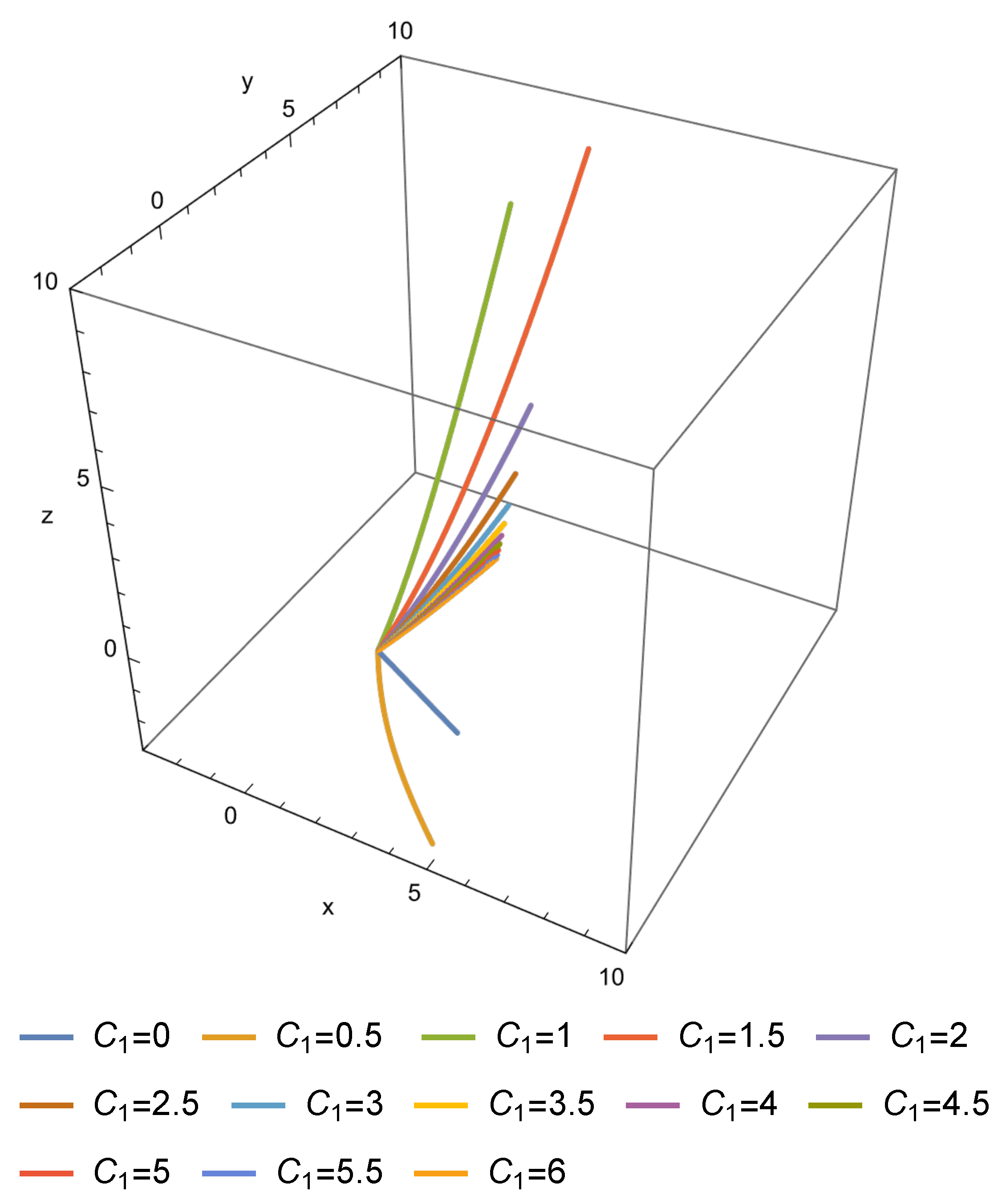
are two linearly independent solutions to Equation (38). As a consequence, a 1-parameter family of solutions to system (23), which corresponds to (37) when $C_2=0,$ can be expressed in terms of the modified Bessel functions as follows:

$$\left\{\begin{array}{ccc}x\left(t\right)\hfill & =\hfill & \pm {\left(\sqrt{2}{\displaystyle \frac{C_1{\mathbf{K}}_1^{\prime }\left(\sqrt{2}t\right)-{\mathbf{I}}_1^{\prime }\left(\sqrt{2}t\right)}{C_1{\mathbf{K}}_1\left(\sqrt{2}t\right)-{\mathbf{I}}_1\left(\sqrt{2}t\right)}}-{\displaystyle \frac{1}{t}}\right)}^{1/2},\hfill \\ y\left(t\right)\hfill & =\hfill & {\displaystyle \frac{1}{2}}+{\displaystyle \frac{\sqrt{2}t}{2}}{\displaystyle \frac{C_1{\mathbf{K}}_1^{\prime }\left(\sqrt{2}t\right)-{\mathbf{I}}_1^{\prime }\left(\sqrt{2}t\right)}{C_1{\mathbf{K}}_1\left(\sqrt{2}t\right)-{\mathbf{I}}_1\left(\sqrt{2}t\right)}}.\hfill \end{array}\right.$$

(42)

The derivatives of the modified Bessel functions ${\mathbf{I}}_1$ and ${\mathbf{K}}_1$ can be expressed in terms of the modified Bessel functions ${\mathbf{I}}_0$ and ${\mathbf{K}}_0$ [56]:

$${\mathbf{K}}_1^{\prime }\left(z\right)={\mathbf{K}}_0\left(z\right)-{\displaystyle \frac{1}{z}}{\mathbf{K}}_1\left(z\right),{\mathbf{I}}_1^{\prime }\left(z\right)={\mathbf{I}}_0\left(z\right)-{\displaystyle \frac{1}{z}}{\mathbf{I}}_1\left(z\right).$$

Then

$${\mathbf{K}}_1^{\prime }\left(\sqrt{2}t\right)=-{\mathbf{K}}_0\left(\sqrt{2}t\right)-{\displaystyle \frac{\sqrt{2}}{2t}}{\mathbf{K}}_1\left(\sqrt{2}t\right),{\mathbf{I}}_1^{\prime }\left(\sqrt{2}t\right)={\mathbf{I}}_0\left(\sqrt{2}t\right)-{\displaystyle \frac{\sqrt{2}}{2t}}{\mathbf{I}}_1\left(\sqrt{2}t\right),$$

and therefore (42) becomes

$$\left\{\begin{array}{ccc}x\left(t\right)\hfill & =\hfill & \pm {\left(\sqrt{2}{\displaystyle \frac{C_1{\mathbf{K}}_0\left(\sqrt{2}t\right)-{\mathbf{I}}_0\left(\sqrt{2}t\right)}{C_1{\mathbf{K}}_1\left(\sqrt{2}t\right)-{\mathbf{I}}_1\left(\sqrt{2}t\right)}}-{\displaystyle \frac{2}{t}}\right)}^{1/2},\hfill \\ y\left(t\right)\hfill & =\hfill & {\displaystyle \frac{\sqrt{2}t}{2}}{\displaystyle \frac{C_1{\mathbf{K}}_0\left(\sqrt{2}t\right)-{\mathbf{I}}_0\left(\sqrt{2}t\right)}{C_1{\mathbf{K}}_1\left(\sqrt{2}t\right)-{\mathbf{I}}_1\left(\sqrt{2}t\right)}}.\hfill \end{array}\right.$$

(43)

In Figure 2, some orbits of the system (23) are plotted by setting particular values to the integration constants $C_1$ and $C_2$.

5. ${\mathcal{C}}^{\mathbf{\infty }}$-Structures for Scalar ODEs with a Lack of Lie Point Symmetries

In this section, we present a collection of ordinary differential equations whose symmetry algebras are either trivial or of lower dimension than the order of the ODE. In the latter scenario, the Lie method encounters certain obstacles when attempting to obtain the general solution. However, we demonstrate how the ${\mathcal{C}}^{\infty }$-structures method successfully overcomes these difficulties and provides exact solutions to the equations under investigation.

5.1. A Third-Order ODE with Two-Dimensional Algebra of Lie Point Symmetries

In this example, we consider a third-order ODE:

$$u_3=(u_1-u)u_2-{\displaystyle \frac{u_1^2}{2}}+u_1+{\displaystyle \frac{u^2}{2}},$$

(44)

whose associated vector field is

$$Z={\partial }_x+u_1{\partial }_u+u_2{\partial }_{u_1}+\left((u_1-u)u_2-\frac{1}{2}(u_1^2-u^2)+u_1\right){\partial }_{u_2}.$$

The symmetry algebra of Equation (44) is two-dimensional and spanned by ${\partial }_x$ and $e^x{\partial }_u$, as can be checked. By employing the Lie method of reduction, the transformation

$$z=u_1-u,h\left(z\right)=u_2-u_1,$$

(45)

leads to the first-order ODE

$$h\left(z\right)h^{\prime }\left(z\right)=(z-1)h\left(z\right)+{\displaystyle \frac{z^2}{2}}.$$

(46)

Equation (46) is an Abel-type equation whose general solution can be expressed in an implicit form in terms of the modified Bessel functions of the first and second kinds ${\mathbf{I}}_{\alpha }$ and ${\mathbf{K}}_{\alpha },$ for $\alpha =0,1$ [56]:

$${\displaystyle \frac{z{\mathbf{K}}_0\left(-\sqrt{z^2-2h\left(z\right)}\right)-\sqrt{z^2-2h\left(z\right)}{\mathbf{K}}_1\left(-\sqrt{z^2-2h\left(z\right)}\right)}{z{\mathbf{I}}_0\left(\sqrt{z^2-2h\left(z\right)}\right)-\sqrt{z^2-2h\left(z\right)}{\mathbf{I}}_1\left(\sqrt{z^2-2h\left(z\right)}\right)}}=C_1.$$

(47)

The recovery of solutions to Equation (44) from (47), by means of the transformation (45), seems to be infeasible.

For this reason, we intend to integrate Equation (44) using the ${\mathcal{C}}^{\infty }$-structures method. Similar to the previous examples, finding the elements of a ${\mathcal{C}}^{\infty }$-structure can be significantly simplified by assuming some of the infinitesimals to be constant or linear in $u_1$. By following this approach, we obtain the following independent vector fields

$$\begin{array}{c}{X}_1={\partial }_u+{\partial }_{u_1}+{\partial }_{u_2},\hfill \\ X_2={\partial }_{u_1}+(u_1-u+1){\partial }_{u_2},\hfill \\ X_3={\partial }_{u_2}.\hfill \end{array}$$

They form a ${\mathcal{C}}^{\infty }$-structure for $\mathcal{S}\left(\right\{Z\left\}\right),$ as can be verified using the Lie brackets:

$$\begin{array}{c}[X_1,Z]=X_1,\hfill \\ [X_2,Z]=X_1+(u_1-u)X_2,\hfill \\ [X_2,X_1]=0.\hfill \end{array}$$

It is important to emphasize that neither $X_1$ is a symmetry of $\mathcal{S}\left(\right\{Z\left\}\right),$ nor $X_2$ is a symmetry of $\mathcal{S}\left(\{Z,X_1\}\right).$ In particular, neither $X_1$ nor $X_2$ correspond to symmetries of Equation (44).

We use the volume form $\mathbf{\Omega }=dx\wedge du\wedge d{u}_1\wedge d{u}_2$ to construct the corresponding 1-forms given in (5):

$$\begin{array}{c}{\omega }_1=-u_{1}dx+du,\hfill \\ {\omega }_2=(u_2-u_1)dx+du-d{u}_1,\hfill \\ {\omega }_3=(u_2+u{u}_1-u_1+\frac{1}{2}(u_1^2+u^2))dx+(u_1-u)du+(u-u_1-1)d{u}_1+d{u}_2.\hfill \end{array}$$

(48)

A first integral for the first Pfaffian equation ${\mathcal{P}}_2,$, i.e., a function $I_3=I_3(x,u,u_1,u_2)$ such that $d{I}_3\wedge {\omega }_3=0$, is given by

$$I_3=e^x\left(u_2-\frac{1}{2}{(u_1-u)}^2-u_1\right).$$

Let ${\Sigma }_{\left(C_3\right)}$ denote, as before, the level set $I_3=C_3,$ for $C_3\in \mathbb{R}.$ The restriction of the 1-form ${\omega }_2$ in (48) to ${\Sigma }_{\left(C_3\right)}$ becomes

$${\omega }_2{|}_{{\Sigma }_{\left(C_3\right)}}=\left(\frac{1}{2}{(u_1-u)}^2+C_3{e}^{-x}\right)dx+du-d{u}_1.$$

(49)

In order to continue the integration process, we need to distinguish the following cases:

• Case I: $C_3>0.$
  It can be checked that a function $I_2=I_2(x,u,u_1;C_3)$ such that $d{I}_2\wedge {\omega }_2{|}_{{\Sigma }_{\left(C_3\right)}}=0$ becomes:

  $$I_2={\displaystyle \frac{e^{x/2}(u_1-u){\mathbf{J}}_0\left(\sqrt{2C_3}{e}^{-x/2}\right)+\sqrt{2C_3}{\mathbf{J}}_1\left(\sqrt{2C_3}{e}^{-x/2}\right)}{e^{x/2}(u-u_1){\mathbf{Y}}_0\left(\sqrt{2C_3}{e}^{-x/2}\right)-\sqrt{2C_3}{\mathbf{Y}}_1\left(\sqrt{2C_3}{e}^{-x/2}\right)}},$$

  where ${\mathbf{J}}_{\alpha },{\mathbf{Y}}_{\alpha }$ are the Bessel functions of the first and second kind, respectively, [56].
  Let ${\Sigma }_{(C_2,C_3)}$ denote the submanifold of ${\Sigma }_{\left(C_3\right)}$ defined by $I_2(x,u,u_1;C_3)=C_2,$ where $C_2\in \mathbb{R}.$ The restriction of the 1-form ${\omega }_3$ in (48) to ${\Sigma }_{(C_2,C_3)}$ becomes

  $${\omega }_1{|}_{{\Sigma }_{(C_2,C_3)}}=\left({\displaystyle \frac{\sqrt{2C_3}{e}^{-x/2}\left(C_2{\mathbf{Y}}_1\left(\sqrt{2C_3}{e}^{-x/2}\right)+{\mathbf{J}}_1\left(\sqrt{2C_3}{e}^{-x/2}\right)\right)}{C_2{\mathbf{Y}}_0\left(\sqrt{2C_3}{e}^{-x/2}\right)+{\mathbf{J}}_0\left(\sqrt{2C_3}{e}^{-x/2}\right)}}-u\right)dx+du.$$
  A function $I_1=I_1(x,u;C_2,C_3)$ such that $d{I}_1\wedge {\omega }_1{|}_{{\Sigma }_{(C_2,C_3)}}=0$ is given by

  $$I_1=\sqrt{2C_3}{\psi }_{(C_2;C_3)}\left(x\right)+e^{-x}u.$$

  where

  $${\psi }_{(C_2;C_3)}^{\prime }\left(x\right)={\displaystyle \frac{C_2{\mathbf{Y}}_1\left(\sqrt{2C_3}{e}^{-x/2}\right)+{\mathbf{J}}_1\left(\sqrt{2C_3}{e}^{-x/2}\right)}{C_2{\mathbf{Y}}_0\left(\sqrt{2C_3}{e}^{-x/2}\right)+{\mathbf{J}}_0\left(\sqrt{2C_3}{e}^{-x/2}\right)}}{e}^{-\frac{3}{2}x}.$$

  (50)
  Finally, the solution of (44) is obtained by setting $I_1(x,u;C_2,C_3)=C_1,$ for $C_1\in \mathbb{R},$ which gives

  $$u\left(x\right)=-\sqrt{2C_3}{e}^x{\psi }_{(C_2;C_3)}\left(x\right)+C_1{e}^x,$$

  where the function ${\psi }_{(C_2;C_3)}$ satisfies (50).
• Case II: $C_3<0.$
  In this case a function $I_2=I_2(x,u,u_1;C_3)$ such that $d{I}_2\wedge {\omega }_2{|}_{{\Sigma }_{\left(C_3\right)}}=0$ is given by:

  $$I_2={\displaystyle \frac{e^{x/2}(u_1-u){\mathbf{I}}_0\left(\sqrt{-2C_3}{e}^{-x/2}\right)-\sqrt{-2C_3}{\mathbf{I}}_1\left(\sqrt{-2C_3}{e}^{-x/2}\right)}{e^{x/2}(u-u_1){\mathbf{K}}_0\left(\sqrt{-2C_3}{e}^{-x/2}\right)-\sqrt{-2C_3}{\mathbf{K}}_1\left(\sqrt{-2C_3}{e}^{-x/2}\right)}}$$

  where ${\mathbf{I}}_{\alpha },{\mathbf{K}}_{\alpha }$ are the modified Bessel functions of the first and second kind, respectively, [56].
  Proceeding as in the previous case, we obtain the following solution to Equation (44):

  $$u\left(x\right)=\sqrt{-2C_3}{e}^x{\phi }_{(C2;C_3)}\left(x\right)+C_1{e}^x,$$

  where

  $${\phi }_{(C2;C_3)}^{\prime }\left(x\right)={\displaystyle \frac{C_2{\mathbf{K}}_1(-\sqrt{-2C_3}{e}^{-x/2})-{\mathbf{I}}_1\left(\sqrt{-2C_3}{e}^{-x/2}\right)}{C_2{\mathbf{K}}_0(-\sqrt{-2C_3}{e}^{-x/2})+{\mathbf{I}}_0\left(\sqrt{-2C_3}{e}^{-x/2}\right)}}{e}^{-\frac{3}{2}x}.$$
• Case III: $C_3=0.$
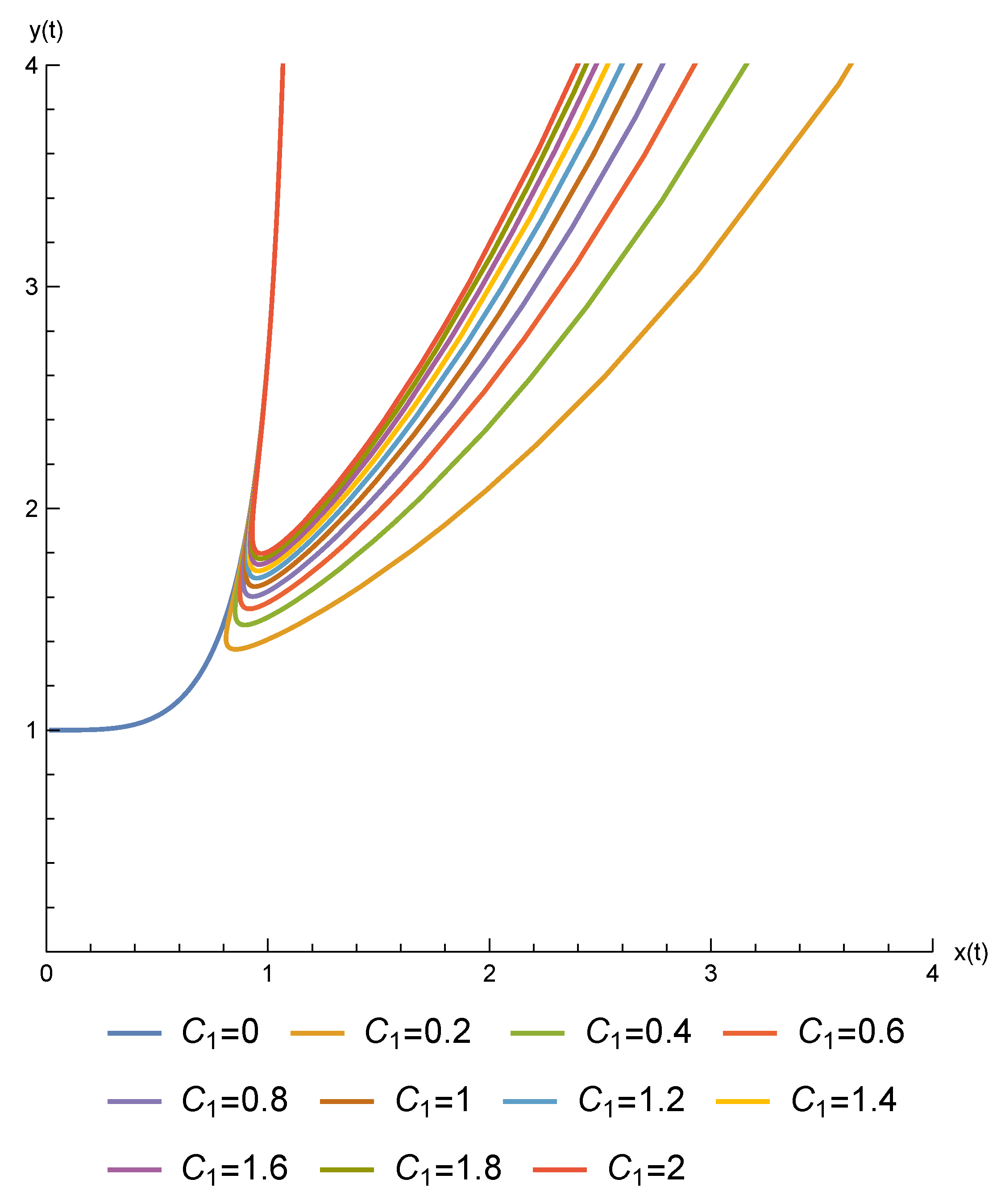
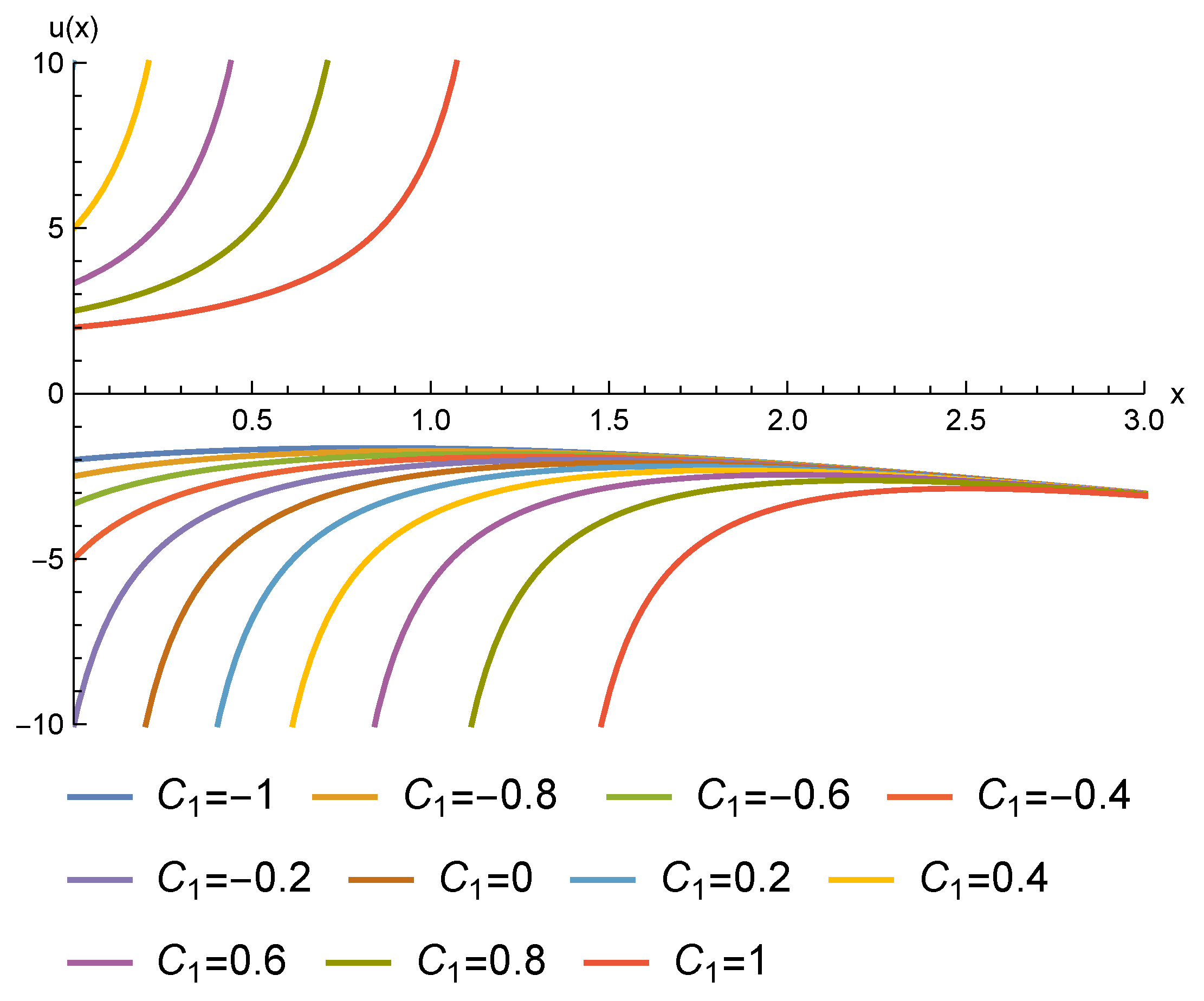
  It can be checked that a solution for the Pfaffian equation defined by the restriction of the 1-form ${\omega }_2$ in (48) to the level set $I_3=0$ is given by

  $$I_2=\frac{x}{2}+\frac{1}{u_1-u}.$$
  The restriction of the 1-form ${\omega }_1$ in (48) to the submanifold ${\Sigma }_{(C_2,0)}$ implicitly defined by $I_3=0,I_2=C_2,$ $C_2\in \mathbb{R}$ becomes

  $${\omega }_1{|}_{{\Sigma }_{(C_2,0)}}=-\left(u+\frac{2}{2C_2-x}\right)dx+du.$$
  The solution of the Pfaffian equation ${\omega }_1{|}_{{\Sigma }_{(C_2,0)}}\equiv 0$ is defined by the function

  $$I_1=u{e}^{-x}-2e^{-2C_2}{E}_1(x-2C_2),$$

  where $E_1=E_1\left(z\right)$ denotes the exponential integral function [56]

  $$E_1\left(z\right)={\int }_z^{\infty }{\displaystyle \frac{e^{-t}}{t}}dt.$$
  By setting $I_1(x,u,C_2)=C_1,$ for $C_1\in \mathbb{R},$ we finally obtain the following 2-parameter family of exact solutions for Equation (44):

  $$u\left(x\right)=2e^{x-2C_2}{E}_1(x-2C_2)+C_1{e}^x.$$

  (51)
  The graphs of some solutions, for different values of the integration constants, are presented in Figure 3:

5.2. A Fourth-Order ODE with a 1-Dimensional Algebra of Lie Point Symmetries

In this subsection, we consider the fourth-order equation

$$u_4=u_1{u}_3+(x^2+1)u_2+u_2^2-\frac{1}{2}(x^2+1)u_1^2,$$

(52)

which has only the Lie point symmetry $\mathbf{v}={\partial }_u$. It can be checked that the Lie reduction method leads to a third-order equation from which it seems difficult to recover the general solution of the initial Equation (52).

By proceeding as in the previous examples, a ${\mathcal{C}}^{\infty }$-structure $\langle X_1,X_2,X_3,X_4\rangle$ for the distribution generated by the vector field

$$Z={\partial }_x+u_1{\partial }_u+u_2{\partial }_{u_1}+u_3{\partial }_{u_2}+\left(u_1{u}_3+(x^2+1)u_2+u_2^2-\frac{1}{2}(x^2+1)u_1^2\right){\partial }_{u_3}$$

can be explicitly determined by the following vector fields:

$$\begin{array}{c}{X}_1={\partial }_u,\hfill \\ X_2={\partial }_{u_1}+u_1{\partial }_{u_2}+(u_1^2+u_2){\partial }_{u_3},\hfill \\ X_3={\partial }_{u_2}+(x+u_1){\partial }_{u_3},\hfill \\ X_4={\partial }_{u_3}.\hfill \end{array}$$

(53)

Since $X_1={\partial }_u={\mathbf{v}}^{\left(3\right)},$ where ${\mathbf{v}}^{\left(3\right)}$ denotes the third-order prolongation of the Lie point symmetry $\mathbf{v}$ [1], it is clear that $X_1$ is a ${\mathcal{C}}^{\infty }$-symmetry of $\mathcal{S}\left(\right\{Z\left\}\right)$ in the sense of Definition 3. The vector field $X_2$ is a ${\mathcal{C}}^{\infty }$-symmetry of $\mathcal{S}\left(\{Z,X_1\}\right)$ because

$$\begin{array}{c}[X_2,Z]=X_1+u_1{X}_2,\hfill \end{array}[X_2,X_1]=0.$$

The vector field $X_3$ is a ${\mathcal{C}}^{\infty }$-symmetry of $\mathcal{S}\left(\{Z,X_1,X_2\}\right)$, since

$$\begin{array}{l}[X_3,Z]=X_2+x{X}_3,\\ [X_3,X_1]=0,\\ [X_3,X_2]=0.\end{array}$$

Finally, X₄ is a ${\mathcal{C}}^{\infty }$-symmetry of $\mathcal{S}$ ({Z, X₁, X₂, X₃}) because {Z, X₁, X₂, X₃} are pointwise linearly independent. In this example, X₂, X₃, and X₄ do not correspond to symmetries of Equation (52).

We use the volume form $\mathbf{\Omega }=dx\wedge du\wedge d{u}_1\wedge d{u}_2\wedge d{u}_3$ to calculate 1-forms given by (5):

$$\begin{array}{c}{\omega }_1=u_{1}dx-du,\hfill \\ {\omega }_2=-u_{2}dx+d{u}_1,\hfill \\ {\omega }_3=-(u_1{u}_2-u_3)dx+u_{1}d{u}_1-d{u}_2,\hfill \\ {\omega }_4=(-u_2(x^2+x{u}_1+1)+\frac{1}{2}(x^2+1)u_1^2+x{u}_3)dx+(x{u}_1-u_2)d{u}_1-(x+u_1)d{u}_2+d{u}_3.\hfill \end{array}$$

• We begin by solving the Pfaffian equation ${\omega }_4\equiv 0$. It can be checked that a smooth function $I_4=I_4(x,u,u_1,u_2,u_3)$ such that $d{I}_4\wedge {\omega }_4=0$ is given by:

  $$I_4=\left(\frac{1}{2}x{u}_1^2-u_1{u}_2-x{u}_2+u_3\right)e^{\frac{1}{2}{x}^2}.$$
• The restriction of ${\omega }_3$ to the submanifold ${\Sigma }_{\left(C_4\right)}$ implicitly defined by $I_4=C_4,$ $C_4\in \mathbb{R},$ becomes

  $${\omega }_3{|}_{{\Sigma }_{\left(C_4\right)}}=\left(-\frac{1}{2}x{u}_1^2+x{u}_2+C_4{e}^{-\frac{1}{2}{x}^2}\right)dx+u_{1}d{u}_1-d{u}_2.$$
  A smooth function $I_3=I_3(x,u,u_1,u_2;C_4)$ such that $d{I}_3\wedge {\omega }_3{|}_{{\Sigma }_{\left(C_4\right)}}=0$ can be expressed in the form:

  $$I_3=-\frac{1}{2}{C}_4\sqrt{\pi }Erf\left(x\right)+\left(u_2-\frac{1}{2}{u}_1^2\right)e^{-\frac{1}{2}{x}^2},$$

  where $\mathrm{Erf}=\mathrm{Erf}\left(z\right)$ denotes the error function defined by [56]

  $$\mathrm{Erf}\left(z\right)={\displaystyle \frac{2}{\sqrt{\pi }}}{\int }_0^z{e}^{-t^2}dt.$$

  (54)
• The restriction of ${\omega }_2$ to the submanifold ${\Sigma }_{(C_3,C_4)}$ of ${\Sigma }_{\left(C_4\right)}$ implicitly defined by $I_3(x,u,u_1,u_2;C_4)=C_3,$ where $C_3\in \mathbb{R},$ becomes

  $${\omega }_2{|}_{{\Sigma }_{(C_3,C_4)}}=-\left(\frac{1}{2}{C}_4\sqrt{\pi }\mathrm{Erf}\left(x\right)e^{\frac{1}{2}{x}^2}+\frac{1}{2}{u}_1^2+C_3{e}^{\frac{1}{2}{x}^2}\right)dx+d{u}_1.$$
  It can be checked that a function $I_2=I_2(x,u,u_1;C_3,C_4)$ such that $d{I}_2\wedge {\omega }_2{|}_{{\Sigma }_{(C_3,C_4)}}=0$ is given by

  $$I_2=-\frac{u_1{\psi }_2(x;C_3,C_4)+2{\psi }_2^{\prime }(x;C_3,C_4)}{u_1{\psi }_1(x;C_3,C_4)+2{\psi }_1^{\prime }(x;C_3,C_4)},$$

  (55)

  where ${\psi }_1={\psi }_1(x;C_3,C_4)$ and ${\psi }_1={\psi }_1(x;C_3,C_4)$ constitute a fundamental set of solutions to the following two-parameter family of Schrödinger-type equations:

  $${\psi }^{\prime \prime }\left(x\right)=-\frac{1}{2}{e}^{\frac{1}{2}{x}^2}\left(\sqrt{\pi }\frac{C_4}{2}\mathrm{Erf}\left(x\right)+C_3\right)\psi \left(x\right).$$

  (56)
• Finally, the restriction of ${\omega }_1$ to the submanifold ${\Sigma }_{(C_2,C_3,C_4)}$ of ${\Sigma }_{(C_3,C_4)}$ defined by $I_2(x,u,u_1;C_3,C_4)=C_2$, with $C_2\in \mathbb{R}$, becomes

  $${\omega }_1{|}_{{\Sigma }_{(C_2,C_3,C_4)}}=\frac{2\left(C_2{\psi }_1^{\prime }(x;C_3,C_4)+{\psi }_2^{\prime }(x;C_3,C_4)\right)}{C_2{\psi }_1(x;C_3,C_4)+{\psi }_2(x;C_3,C_4)}dx+du.$$
  A function $I_1=I_1(x,u;C_2,C_3,C_4)$ such that $d{I}_1\wedge {\omega }_1{|}_{{\Sigma }_{(C_2,C_3,C_4)}}=0$ can be calculated by a simple quadrature and becomes

  $$I_1=u+2ln\left(C_2{\psi }_1(x;C_3,C_4)+{\psi }_2(x;C_3,C_4)\right).$$

As a result of the previous procedure of integration, using the ${\mathcal{C}}^{\infty }$-structure defined by (53), the initial fourth-order Equation (52) has been completely integrated. A fundamental set of solutions of ${\psi }_1(x;C_3,C_4)$ and ${\psi }_2(x;C_3,C_4)$ of (56) can be used to express the general solution of the given problem in the form:

$$u\left(x\right)=-2ln\left(C_2{\psi }_1(x;C_3,C_4)+{\psi }_2(x;C_3,C_4)\right)+C_1,$$

(57)

where $C_i\in \mathbb{R}$ for $i=1,2,3,4.$

Some Particular Solutions in Terms of Elementary Functions

For some particular values of the arbitrary constants in (57), the general solution to Equation (52) can be expressed in terms of elementary functions. This is the case, for instance, when $C_3=C_4=0.$ For these particular values, the Schrödinger-type Equation (56) turns out to be simply ${\psi }^{″}=0$ and therefore a corresponding fundamental set of solutions is given by ${\psi }_1\left(x\right)=1$ and ${\psi }_2\left(x\right)=x.$

In this case, the expression (57) provides the following two-parameter familiy of exact solutions for Equation (44):

$$u\left(x\right)=-2ln(x+C_2)+C_1,C_1,C_2\in \mathbb{R}.$$

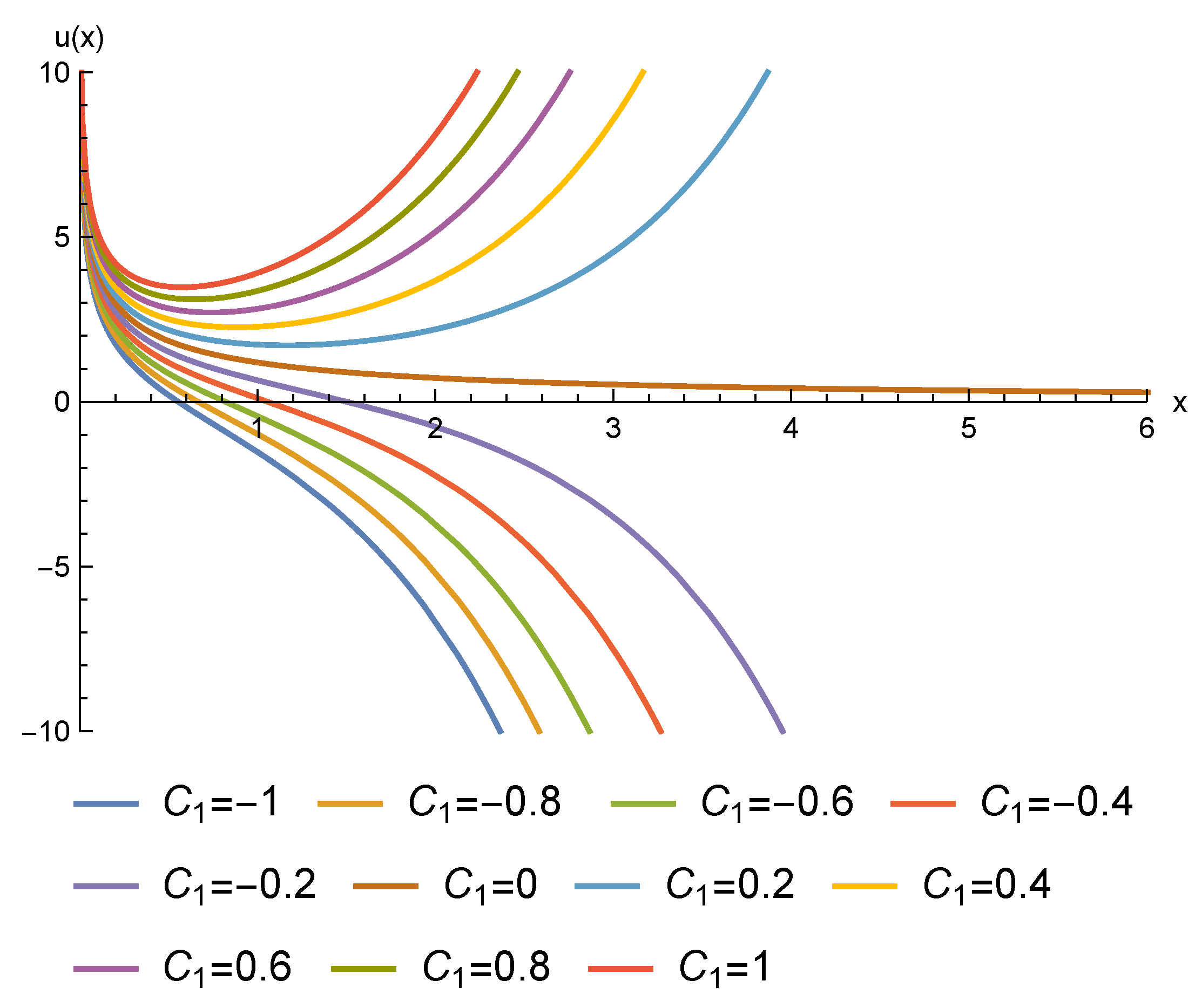
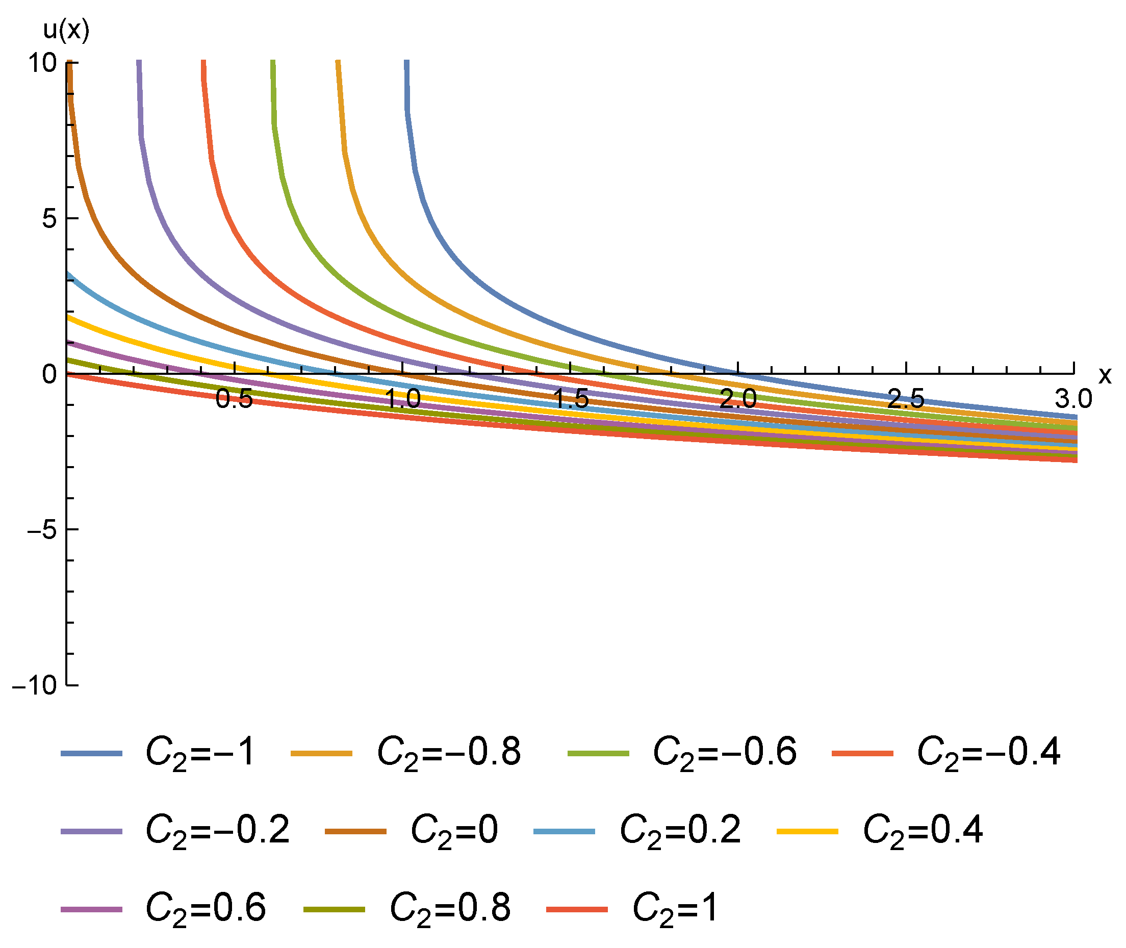
The graphs of some solutions of this type are plotted in Figure 4:

5.3. A Fourth-Order ODE without Lie Point Symmetries

This example illustrates the success of the ${\mathcal{C}}^{\infty }$-structure-based method in solving ODEs for which the classical Lie method cannot be applied due to the absence of Lie point symmetries in the equation. This is the case of the fourth-order ODE

$$u_4=-u{u}_1+u{u}_3+3u_1{u}_2+x+u_2,$$

(58)

whose associated vector field is

$$Z={\partial }_x+u_1{\partial }_u+u_2{\partial }_{u_1}+u_3{\partial }_{u_2}+\left(-u{u}_1+u{u}_3+3u_1{u}_2+x+u_2\right){\partial }_{u_3}.$$

It can be checked that the determining equations for a Lie point symmetry of Equation (58), in the form $v=\xi (x,u){\partial }_x+\eta (x,u){\partial }_u$, yield the trivial solution $\xi =\eta =0$. Therefore Equation (58) does not admit Lie point symmetries.

Finding a ${\mathcal{C}}^{\infty }$-structure for $\mathcal{S}\left(\right\{Z\left\}\right)$ can be simplified by assuming that some of the infinitesimals of the corresponding elements are constant or linear with respect to $u_1$ and $u_2$. This is similar to the approach used in the previous examples. In this way, we find the ordered set $\langle X_1,X_2,X_3,X_4\rangle$ given by the following vector fields:

$$\begin{array}{c}{X}_1={\partial }_u+u{\partial }_{u_1}+(u^2+u_1){\partial }_{u_2}+(u^3+3u{u}_1+u_2){\partial }_{u_3},\hfill \\ X_2={\partial }_{u_1}+u{\partial }_{u_2}+(u^2+2u_1){\partial }_{u_3},\hfill \\ X_3={\partial }_{u_2}+(u-1){\partial }_{u_3},\hfill \\ X_4={\partial }_{u_3}.\hfill \end{array}$$

It can be verified that the vector field $X_1$ is a ${\mathcal{C}}^{\infty }$-symmetry of $\mathcal{S}\left(\right\{Z\left\}\right)$, since $[X_1,Z]=u{X}_1$. On the other hand, the vector field $X_2$ is a symmetry of $\mathcal{S}\left(\{Z,X_1\}\right)$, because

$$\begin{array}{c}[X_2,Z]=X_1,\hfill \\ [X_2,X_1]=0.\hfill \end{array}$$

Finally X₃ is a ${\mathcal{C}}^{\infty }$-symmetry of $\mathcal{S}$({Z, X1, X2}), since the following commutation relations are satisfied:

$$\begin{array}{c}[X_3,Z]=X_2-X_3,\hfill \\ [X_3,X_1]=0.\hfill \\ [X_3,X_2]=0.\hfill \end{array}$$

Thus, in accordance with Definition 4, and considering the pointwise linear independence of X₁, X₂, X₃, X₄, the ordered set $\langle X_1,X_2,X_3,X_4\rangle$ forms a ${\mathcal{C}}^{\infty }$-structure for $\mathcal{S}$(Z).

In what follows, we employ the integration method outlined in Section 3 to achieve our objective of solving Equation (58). The corresponding 1-forms provided in (5) yield the following expression when using $\mathbf{\Omega }=dx\wedge du\wedge d{u}_1\wedge d{u}_2\wedge d{u}_3:$

$$\begin{array}{cc}{\omega }_1=& u_{1}dx-du,\hfill \\ {\omega }_2=& (u{u}_1-u_2)dx-udu+d{u}_1,\hfill \\ {\omega }_3=& -(u{u}_2+u_1^2-u_3)dx+u_{1}du+ud{u}_1-d{u}_2,\hfill \\ {\omega }_4=& -(-u{u}_1-u{u}_2-u_1^2+x+u_2+u_3)dx-(u_1+u_2)du-(u+2u_1)d{u}_1\hfill \\ & +(1-u)d{u}_2+d{u}_3.\hfill \end{array}$$

(59)

The results obtained after applying the integration procedure, as described in Section 3, are presented below.

• The Pfaffian equation ${\omega }_4\equiv 0$ is completely integrable and a function $I_4=I_4(x,u,u_1,u_2,u_3)$ such that $d{I}_4\wedge {\omega }_4=0$ can be chosen as

  $$I_4=(-u_1^2-u_{1}u-(u-1)u_2+x+u_3+1)e^{-x}.$$
• The restriction of the 1-form ${\omega }_3$ given in (59) to ${\Sigma }_{\left(C_4\right)}$ provides

  $${\omega }_3{|}_{{\Sigma }_{\left(C_4\right)}}=(C_4{e}^x+u_{1}u-x-u_2-1)dx+u_{1}du+ud{u}_1-d{u}_2.$$
  A function $I_3=I_3(x,u,u_1,u_2;C_4)$ such that $d{I}_3\wedge {\omega }_3{|}_{{\Sigma }_{\left(C_4\right)}}=0$ is

  $$I_3=-\frac{1}{2}{C}_4{e}^{2x}-e^x(u{u}_1-x-u_2).$$
• We now restrict the 1-form ${\omega }_2$ in (59) to ${\Sigma }_{(C_3,C_4)},$ resulting in

  $${\omega }_2{|}_{{\Sigma }_{(C_3,C_4)}}=-\left(\frac{1}{2}{C}_4{e}^x-x+C_3{e}^{-x}\right)dx-udu+d{u}_1.$$
  A function $I_2=I_2(x,u,u_1;C_3,C_4)$ such that $d{I}_2\wedge {\omega }_3{|}_{{\Sigma }_{(C_3,C_4)}}=0$ can be calculated by simple quadrature:

  $$I_2=-\frac{1}{2}{C}_4{e}^x+\frac{1}{2}{x}^2-\frac{1}{2}{u}^2+u_1+C_3{e}^{-x}.$$
• Finally, the restriction of the 1-form ${\omega }_1$ given in (59) to ${\Sigma }_{(C_2,C_3,C_4)}$ turns out to be:

  $${\omega }_1{|}_{{\Sigma }_{(C_2,C_3,C_4)}}=\left(\frac{1}{2}{u}^2+\frac{1}{2}{C}_4{e}^x-\frac{1}{2}{x}^2-C_3{e}^{-x}+C_2\right)dx-du.$$

  (60)
  The integration of the Pfaffian equation ${\omega }_1{|}_{{\Sigma }_{(C_2,C_3,C_4)}}\equiv 0$ is equivalent to solve the following first-order ODE:

  $$u_1=\frac{1}{2}{u}^2+\frac{1}{2}{C}_4{e}^x-\frac{1}{2}{x}^2-C_3{e}^{-x}+C_2,$$

  (61)

  which is of Riccati-type. Equation (61) can be mapped into the following Schrödinger-type equation by means of the standard transformation $u=-2{\psi }^{\prime }\left(x\right)/\psi \left(x\right)$:

  $${\psi }^{\prime \prime }\left(x\right)=\left(\frac{1}{4}{x}^2-\frac{1}{4}{C}_4{e}^x+\frac{1}{2}{C}_3{e}^{-x}-\frac{1}{2}{C}_2\right)\psi \left(x\right).$$

  (62)
  Therefore, if ${\psi }_1={\psi }_1(x;C_2,C_3,C_4)$ and ${\psi }_2={\psi }_2(x;C_2,C_3,C_4)$ form a fundamental set of solutions to Equation (62), a first integral $I_1=I_1(x,u;C_2,C_3,C_4)$ for the Riccati Equation (61) is given by ([55] Proposition 4.1)

  $$I_1={\displaystyle \frac{u{\psi }_1(x;C_2,C_3,C_4)+2{\psi }_1^{\prime }(x;C_2,C_3,C_4)}{u{\psi }_2(x;C_2,C_3,C_4)+2{\psi }_2^{\prime }(x;C_2,C_3,C_4)}}$$

  (63)

By setting $I_1(x,u;C_2,C_3,C_4)=C_1,$ where $C_1\in \mathbb{R},$ we obtain the general solution for Equation (58), expressed in terms of a fundamental set of solutions to Equation (62):

$$u\left(x\right)=\frac{-2\left(C_1{\psi }_1^{\prime }(x;C_2,C_3,C_4)+{\psi }_2^{\prime }(x;C_2,C_3,C_4)\right)}{C_1{\psi }_1(x;C_2,C_3,C_4)+{\psi }_2(x;C_2,C_3,C_4)},$$

(64)

where $C_i\in \mathbb{R}$, for $i=1,2,3,4.$ In consequence, the ${\mathcal{C}}^{\infty }$-structure approach successfully solves the fourth-order Equation (58), despite the absence of Lie point symmetries.

Some Families of Exact Solutions in Terms of Special Functions

For particular values of the constants $C_2,C_3$, and $C_4$ appearing in (62), a fundamental set of solutions to the Schrödinger-type Equation (62) can be expressed in terms of well-known special functions. For instance, when $C_3=C_4=0,$ Equation (62) becomes

$${\psi }^{″}\left(x\right)=\left(\frac{1}{4}{x}^2-\frac{1}{2}{C}_2\right)\psi \left(x\right),$$

which admits the following linearly independent solutions:

$${\psi }_1(x;C_2)={\displaystyle \frac{{\mathbf{W}}_{\frac{1}{4}{C}_2,\frac{1}{4}}\left(\frac{x^2}{2}\right)}{\sqrt{x}}},{\psi }_2(x;C_2)={\displaystyle \frac{{\mathbf{M}}_{\frac{1}{4}{C}_2,\frac{1}{4}}\left(\frac{x^2}{2}\right)}{\sqrt{x}}},$$

(65)

where ${\mathbf{M}}_{\mu ,\nu }={\mathbf{M}}_{\mu ,\nu }\left(z\right)$ and ${\mathbf{W}}_{\mu ,\nu }={\mathbf{W}}_{\mu ,\nu }\left(z\right)$ denotes the corresponding Whittaker functions [56], i.e., two linearly independent solutions to the equation

$${\varphi }^{″}\left(z\right)+\left({\displaystyle \frac{-1}{4}}+{\displaystyle \frac{\mu }{z}}+{\displaystyle \frac{{\displaystyle \frac{1}{4}}-{\nu }^2}{z^2}}\right)\varphi \left(z\right)=0.$$

Therefore, a two-parameter family of solutions that corresponds to (64) when $C_3=C_4=0,$ is given by

$$u\left(x\right)=\frac{-x^2+C_2+1}{x}+\frac{4C_1{\mathbf{W}}_{\frac{1}{4}{C}_2+1,\frac{1}{4}}\left(\frac{1}{2}{x}^2\right)-\left(C_2+3\right){\mathbf{M}}_{\frac{1}{4}{C}_2+1,\frac{1}{4}}\left(\frac{1}{2}{x}^2\right)}{x\left(C_1{\mathbf{W}}_{\frac{1}{4}{C}_2,\frac{1}{4}}\left(\frac{1}{2}{x}^2\right)+{\mathbf{M}}_{\frac{1}{4}{C}_2,\frac{1}{4}}\left(\frac{1}{2}{x}^2\right)\right)}.$$

(66)

Since Whittaker functions can be defined in terms of hypergeometric or Kummer functions, the family of solutions (66) could have alternatively been expressed using other special functions. Furthermore, by selecting different values for $C_2$ in (66), we can generate 1-parameter families of solutions that involve various types of special functions, such as the following examples:

• For $C_2=0,$ (66) provides the next 1-parameter family of exact solutions

  $$u\left(x\right)=-x\frac{C_1{\mathbf{I}}_{-\frac{3}{4}}\left(\frac{1}{4}{x}^2\right)-{\mathbf{K}}_{\frac{3}{4}}\left(\frac{1}{4}{x}^2\right)}{C_1{\mathbf{I}}_{\frac{1}{4}}\left(\frac{1}{4}{x}^2\right)+{\mathbf{K}}_{\frac{1}{4}}\left(\frac{1}{4}{x}^2\right)},$$

  (67)

  where ${\mathbf{I}}_{\nu }$ and ${\mathbf{K}}_{\nu }$ denote the modified Bessel functions of the first and second kinds, respectively.
• When $C_2=-1,$ we obtain the following 1-parameter family of exact solutions for Equation (52):

  $$u\left(x\right)=-x+\frac{4e^{-\frac{1}{2}{x}^2}}{2C_1-\sqrt{2\pi }Erf\left(\frac{1}{2}\sqrt{2}x\right)},$$

  (68)

  where $Erf$ denotes the error function (54).

Several particular solutions for Equation (52) of the type (68) are plotted in Figure 5:

6. Concluding Remarks

In this work, the effectiveness of the ${\mathcal{C}}^{\infty }$-structure procedure as a novel tool to deal with integrability problems in differential equations has been demonstrated. By applying the integration method based on ${\mathcal{C}}^{\infty }$-structures, several models have been fully integrated, including a Lotka–Volterra model and equations for which the Lie method encounters certain obstacles when trying to obtain the general solution.

Consequently, ${\mathcal{C}}^{\infty }$-structures offer significant contributions to solving problems that cannot be solved by classical methods, expanding our understanding and analytical capabilities in tackling intricate mathematical problems.

References

- Olver, P.J. Applications of Lie Groups to Differential Equations; Springer: New York, NY, USA, 1986; Volume 107. [Google Scholar]
- Ovsiannikov, L.V. Group Analysis of Differential Equations; Academic Press: New York, NY, USA, 2014. [Google Scholar]
- Stephani, H. Differential Equations: Their Solutions Using Symmetry; Cambridge University Press: New York, NY, USA, 1989. [Google Scholar]
- Bluman, G.W.; Anco, S.C. Symmetry and Integration Methods for Differential Equations; Springer: New York, NY, USA, 2002. [Google Scholar]
- Basarab-Horwath, P. Integrability by quadratures for systems of involutive vector fields. Ukrainian Math. J. 1991, 43, 1330–1337. [Google Scholar] [CrossRef]
- Hartl, T.; Athorne, C. Solvable structures and hidden symmetries. J. Phys. A Math. Gen. 1994, 27, 3463. [Google Scholar] [CrossRef]
- Sherring, J.; Prince, G. Geometric aspects of reduction of order. Trans. Amer. Math. Soc. 1992, 334, 433–453. [Google Scholar] [CrossRef]
- Barco, M.A.; Prince, G. Solvable symmetry structures in differential form applications. Acta Appl. Math. 2001, 66, 89–121. [Google Scholar] [CrossRef]
- Muriel, C.; Romero, J.L. New methods of reduction for ordinary differential equations. IMA J. Appl. Math. 2001, 66, 111–125. [Google Scholar] [CrossRef]
- Gaeta, G.; Morando, P. On the geometry of λ-symmetries and PDE reduction. J. Phys. A Math. Gen. 2004, 37, 6955–6975. [Google Scholar] [CrossRef]
- Cicogna, G.; Gaeta, G.; Morando, P. On the relation between standard and μ-symmetries for PDEs. J. Phys. A Math. Gen. 2004, 37, 9467–9486. [Google Scholar] [CrossRef]
- Morando, P. Deformation of Lie Derivative and μ-symmetries. J. Phys. A Math. Theor. 2007, 40, 11547–11559. [Google Scholar] [CrossRef]
- Gaeta, G. Twisted symmetries of differential equations. J. Nonlinear Math. Phys. 2009, 16, 107–136. [Google Scholar] [CrossRef]
- Cicogna, G. Reduction of systems of first-order differential equations via Λ-symmetries. Phys. Lett. A 2008, 372, 3672–3677. [Google Scholar] [CrossRef]
- Cicogna, G. Symmetries of Hamiltonian equations and Λ-constants of motion. J. Nonlinear Math. Phys. 2009, 16, 43–60. [Google Scholar] [CrossRef]
- Cicogna, G.; Gaeta, G.; Walcher, S. Dynamical systems and σ-symmetries. J. Phys. A Math. Theor. 2013, 46, 235204. [Google Scholar] [CrossRef]
- Cicogna, G.; Gaeta, G.; Walcher, S. A generalization of λ-symmetry reduction for systems of ODEs: σ-symmetries. J. Phys. A Math. Theor. 2012, 45. [Google Scholar] [CrossRef]
- Levi, D.; Rodríguez, M. λ-symmetries for discrete equations. J. Phys. A Math. Gen. 2010, 43, 292001. [Google Scholar] [CrossRef]
- Levi, D.; Nucci, M.; Rodríguez, M. λ-symmetries for the reduction of continuous and discrete equations. Acta Appl. Math. 2012, 122, 311–321. [Google Scholar] [CrossRef]
- Muriel, C.; Romero, J.L.; Olver, P.J. Variational C∞-symmetries and Euler-Lagrange equations. J. Diff. Eq. 2006, 222, 164–184. [Google Scholar] [CrossRef]
- Cicogna, G.; Gaeta, G. Noether theorem for μ-symmetries. J. Phys. A Math. Theor. 2007, 40, 11899–11921. [Google Scholar] [CrossRef]
- Ruiz, A.; Muriel, C.; Olver, P.J. On the commutator of C∞-symmetries and the reduction of Euler-Lagrange equations. J. Phys. A Math. Theor. 2018, 51, 145202–145223. [Google Scholar] [CrossRef]
- Nadjafikhah, M.; Dodangeh, S.; Kabi-Nejad, P. On the variational problems without having desired variational symmetries. J. Math. 2013, 2013, 685212. [Google Scholar] [CrossRef]
- Morando, P.; Sammarco, S. Variational problems with symmetry: A Pfaffian system approach. Acta Appl. Math. 2012, 120, 255–274. [Google Scholar] [CrossRef]
- Ruiz, A.; Muriel, C. Variational λ-symmetries and exact solutions to Euler–Lagrange equations lacking standard symmetries. Math. Methods Appl. Sci. 2022, 45, 10946–10958. [Google Scholar] [CrossRef]
- Bhuvaneswari, A.; Kraenkel, R.; Senthilvelan, M. Application of the λ-symmetries approach and time independent integral of the modified Emden equation. Nonlinear Anal.-Real World Appl. 2012, 13, 1102–1114. [Google Scholar] [CrossRef]
- Abdel Kader, A.; Abdel Latif, M.; Nour, H. Exact solutions of a third-order ODE from thin film flow using λ-symmetry method. Int. J. Non Linear Mech. 2013, 55, 147–152. [Google Scholar] [CrossRef]
- Guha, P.; Choudhury, A.G.; Khanra, B. λ-Symmetries, isochronicity and integrating factors of nonlinear ordinary differential equations. J. Eng. Math. 2013, 82, 85–99. [Google Scholar] [CrossRef]
- Gün, G.; Özer, T. First integrals, integrating factors, and invariant solutions of the path equation based on Noether and λ-symmetries. Abstr. Appl. Anal. 2013, 2013, 284653. [Google Scholar] [CrossRef]
- Gün, G.; Özer, T. On analysis of nonlinear dynamical systems via methods connected with λ-symmetry. Nonlinear Dyn. 2016, 85, 1571–1595. [Google Scholar] [CrossRef]
- Jafari, H.; Goodarzi, K.; Khorshidi, M.; Parvaneh, V.; Hammouch, Z. Lie symmetry and μ-symmetry methods for nonlinear generalized Camassa–Holm equation. Adv. Differ. Equ. 2021, 2021, 322. [Google Scholar] [CrossRef]
- Kozlov, R. On first integrals of ODEs admitting λ-symmetries. AIP Conf. Proc. 2015, 1648, 430005. [Google Scholar] [CrossRef]
- Mendoza, J.; Muriel, C.; Ramírez, J. New optical solitons of Kundu-Eckhaus equation via λ-symmetry. Chaos Solit. Fractals 2020, 136, 109786. [Google Scholar] [CrossRef]
- Mendoza, J.; Muriel, C. New exact solutions for a generalised Burgers-Fisher equation. Chaos Solit. Fractals 2021, 152, 111360. [Google Scholar] [CrossRef]
- Mohanasubha, R.; Chandrasekar, V.; Senthilvelan, M. A method of identifying integrability quantifiers from an obvious λ-symmetry in second-order nonlinear ordinary differential equations. Int. J. Non-Linear Mech. 2019, 116, 318–323. [Google Scholar] [CrossRef]
- Orhan, O.; Özer, T. On μ-symmetries, μ-reductions, and μ-conservation laws of Gardner equation. J. Nonlinear Math. Phys. 2019, 26, 69–90. [Google Scholar] [CrossRef]
- Ruiz, A.; Muriel, C. On the integrability of Liénard I-type equations via λ-symmetries and solvable structures. Appl. Math. Comput. 2018, 339, 888–898. [Google Scholar] [CrossRef]
- Ruiz, A.; Muriel, C.; Ramírez, J. Parametric Solutions to a Static Fourth-Order Euler–Bernoulli Beam Equation in Terms of Lamé Functions. In Recent Advances in Pure and Applied Mathematics; Springer International Publishing: Cham, Switzerland, 2020; pp. 93–103. [Google Scholar] [CrossRef]
- Zhang, J.; Li, Y. Symmetries and first integrals of differential equations. Acta Appl. Math. 2008, 103, 147–159. [Google Scholar] [CrossRef]
- Muriel, C.; Romero, J.L. C∞-Symmetries and reduction of equations without Lie point symmetries. J. Lie Theory 2003, 13, 167–188. [Google Scholar]
- Cimpoiasu, R.; Cimpoiasu, V. λ-symmetry reduction for nonlinear ODEs without Lie symmetries. Ann. Univ. Craiova Phys. 2015, 25, 22–26. [Google Scholar]
- Pan-Collantes, A.J.; Ruiz, A.; Muriel, C.; Romero, J.L. C∞-symmetries of distributions and integrability. J. Diff. Equ. 2023, 348, 126–153. [Google Scholar] [CrossRef]
- Pan-Collantes, A.J.; Ruiz, A.; Muriel, C.; Romero, J.L. C∞-structures in the integration of involutive distributions. Phys. Scr. 2023, 98, 085222. [Google Scholar] [CrossRef]
- Ibragimov, N.H. A Practical Course in Differential Equations and Mathematical Modelling: Classical and New Methods, Nonlinear Mathematical Models, Symmetry and Invariance Principles; World Scientific: Beijing, China, 2010. [Google Scholar]
- Warner, F.W. Foundations of Differentiable Manifolds and Lie Groups; Springer: New York, NY, USA, 1983; Volume 94. [Google Scholar]
- Bryant, R.L.; Chern, S.S.; Gardner, R.B.; Goldschmidt, H.L.; Griffiths, P.A. Exterior Differential Systems; Springer: New York, NY, USA, 2013; Volume 18. [Google Scholar]
- Duzhin, S.; Lychagin, V.V. Symmetries of Distributions and Quadrature of Ordinary Differential Equations. Acta Appl. Math. 1991, 29, 29–57. [Google Scholar] [CrossRef]
- Kushner, A.; Lychagin, V.; Rubtsov, V. Contact Geometry and Nonlinear Differential Equations; Encyclopedia of Mathematics and Its Applications; Cambridge University Press: Cambridge, UK, 2006. [Google Scholar] [CrossRef]
- Barco, M.A. Solvable structures and their application to a class of Cauchy problem. Eur. J. Appl. Math. 2002, 13, 449–477. [Google Scholar] [CrossRef]
- Morando, P.; Muriel, C.; Ruiz, A. General solvable structures and first integrals for ODEs admitting an sl(2,ℝ) symmetry algebra. J. Nonlinear Math. Phys. 2019, 26, 188–201. [Google Scholar] [CrossRef]
- Takeuchi, Y. Global Dynamical Properties of Lotka-Volterra Systems; World Scientific: Singapore, 1996. [Google Scholar] [CrossRef]
- Grammaticos, B.; Moulin-Ollagnier, J.; Ramani, A.; Strelcyn, J.; Wojciechowski, S. Integrals of quadratic ordinary differential equations in R3: The Lotka-Volterra system. Phys. A Stat. Mech. Appl. 1990, 163, 683–722. [Google Scholar] [CrossRef]
- Solomon, S. Generalized Lotka-Volterra (GLV) models of stock markets. Adv. Complex Syst. 2000, 3, 301–322. [Google Scholar] [CrossRef]
- Maier, R.S. The integration of three-dimensional Lotka–Volterra systems. Proc. Math. Phys. Eng. Sci. 2013, 469, 20120693. [Google Scholar] [CrossRef]
- Ruiz, A.; Muriel, C. First integrals and parametric solutions of third-order ODEs admitting (2,ℝ). J. Phys. A Math. Theor. 2017, 50, 205201. [Google Scholar] [CrossRef]
- Olver, F.W.; Lozier, D.W.; Boisvert, R.F.; Clark, C.W. NIST Handbook of Mathematical Functions Hardback and CD-ROM; Cambridge University Press: Cambridge, UK, 2010. [Google Scholar]
Disclaimer/Publisher’s Note: The statements, opinions and data contained in all publications are solely those of the individual author(s) and contributor(s) and not of MDPI and/or the editor(s). MDPI and/or the editor(s) disclaim responsibility for any injury to people or property resulting from any ideas, methods, instructions or products referred to in the content. |
© 2023 by the authors. Licensee MDPI, Basel, Switzerland. This article is an open access article distributed under the terms and conditions of the Creative Commons Attribution (CC BY) license (https://creativecommons.org/licenses/by/4.0/).
Share and Cite
MDPI and ACS Style
Pan-Collantes, A.J.; Muriel, C.; Ruiz, A.
Integration of Differential Equations by
AMA Style
Pan-Collantes AJ, Muriel C, Ruiz A.
Pan-Collantes, Antonio Jesús, Concepción Muriel, and Adrián Ruiz.
2023. "Integration of Differential Equations by
Note that from the first issue of 2016, this journal uses article numbers instead of page numbers. See further details here.